Microclimate Air Motion and Uniformity of Indoor Plant Factory System: Effects of Crop Planting Density and Air Change Rate

Abstract

In a plant factory, maintaining proper and uniform air/moisture movement above the crop canopy is crucial for aiding plant growth. This research has utilized a three-dimensional computation model to investigate airflow and heat transfer in a plant factory, where airflow, heat, and humidity distributions above plant crops were calculated concerning five categories of crop planting density (P_d) and air change rate (ACH) in the crop area. Spatial uniformities of airflow velocity, temperature, and relative humidity immediately above the crops are evaluated using the objective uniformity parameter (OU), relative standard deviation of temperature (RSD_T) and relative standard deviation of relative humidity (RSD_RH), respectively. Furthermore, a factor of effectiveness (θ) is defined, depending on the uniformity of velocity, temperature, and relative humidity distribution, to comprehensively evaluate the impact of various ACH with P_d on overall effectiveness. Full numerical results show that air velocity, temperature, and relative humidity above the crops are notably influenced by P_d and ACH. As ACH increases, the OU of the air above the indoor crop also expands. Moreover, higher OU values are observed for smaller crop P_d. However, excessively small crop area planting densities and excessively large ACH do not result in a higher OU for the air above the crop. As ACH increases, both RSD_T and RSD_RH decay for the whole range of crop P_d. Moreover, smaller P_d values could achieve the uniformity of thermal fields, while having minimal effects on the relative humidity distributions. Generally, increasing ACH and decreasing P_d could enhance overall value of θ. However, excessively increasing ACH and decreasing P_d does not have a significant effect on θ, which is jointly influenced by OU, RSD_T, and RSD_RH. Therefore, a more suitable combination of ACH and P_d is urgently required to improve the design of agricultural system to enhance crop microclimate uniformity for optimal plant growth and productivity.

1. Introduction

Agriculture always serves as the foundation of human society, driving both population growth and societal advancements. However, rapid urbanization [1], population explosion, uneven distribution of water resources, and the threat of extreme weather [2,3] have negatively impacted traditional agricultural practices [4]. Furthermore, food consumption per capita worldwide has been steadily rising [5]. Thus, ensuring a stable food supply is crucial for people’s daily lives and social activities. To meet the escalating demand for food, it becomes imperative to explore methods to enhance food production. While expanding arable land or increasing yields on existing land seems like viable options, the availability of arable land is diminishing [6]. Therefore, there is a need to prioritize the development of new technologies [7,8] that can achieve higher yields and ensure food security. In this context, plant factories have emerged as a promising alternative [9] to address the challenges of shrinking arable land and increasing food production.

Plant factory is a new facility which could be used for agricultural production with simple control of the indoor environment and has gained widespread attention for its high and stable rate of utilization of resources per unit. In the plant factory closed or semi-closed condition, the indoor environment in the plant factory could adjust the system to achieve accurate control of light, temperature, humidity, nutrient solution, and other parameters in the process of plant growth, so that the plant grows almost unaffected by the external environment to achieve high yield. Indoor ventilation plays a vital role in maintaining a healthy environment in plant factories. Poorly designed ventilation systems can negatively affect air quality in the crop canopy of cultivation trays, ultimately affecting crop growth and yield [10]. Stagnant airflow within the crop canopy is particularly detrimental to plant growth [11]. Therefore, it is important to ensure proper airflow and ventilation within the plant factory to create favorable conditions for crop growth and optimize productivity. The airflow above the crop is crucial for promoting optimal plant growth in plant factories [12].

Former research has demonstrated the significance of well-organized airflow in enhancing crop development. For instance, Shibuya et al. (1998) found that the photosynthetic rate of tomato seedlings increased by 1.9 times when exposed to a wind speed of 0.6 m/s compared to 0.1 m/s [13]. Korthals et al. (1994) conducted a study and observed that soybean plants exposed to an air velocity of 0.8 m/s showed a 14% increase in fresh weight compared to those exposed to an air velocity of 0.4 m/s [14]. This demonstrates the positive impact of higher air velocities on plant growth in a plant factory setting. Furthermore, air temperature and relative humidity are crucial factors that significantly influence plant growth and development [15,16]. The air temperature above the crop has a direct effect on the relative humidity in the surrounding air. Maintaining higher relative humidity levels can effectively reduce the occurrence of leaf tip burn in crop leaves [17]. These findings emphasize the importance of controlling air temperature and relative humidity within the plant factory to create an optimal growth environment for crops.

Computational fluid dynamics (CFD) has emerged as a reliable numerical method for simulating and predicting fluid flow and heat transfer phenomena [18]. It utilizes the finite volume method to solve the governing equations and has proven to be an effective tool in various fields, including agriculture. In agricultural research, CFD is extensively employed by scientists to investigate indoor ventilation processes [16,19,20,21]. In the study of plant factory ventilation design, researchers focus on achieving uniform indoor airflow distribution and crop canopy climate.

Lim et al. (2014) conducted a study and found that the layout of inlet and outlet positions significantly influenced the airflow pattern in plant factories with multi-story cultivation racks, given a specific inlet air supply [22]. Similarly, Noh et al. (2021) utilized CFD to analyze airflow characteristics and temperature distribution in a plant factory. They investigated different inlet and outlet locations while maintaining a uniform air supply volume. By adjusting the air inlet location, they were able to improve the uniformity of airflow and temperature distribution within the plant factory [23]. The utilization of perforated air tubes and optimized ventilation design has been found to improve airflow uniformity and create favorable conditions for crop growth in plant factories. Ying et al. (2016) conducted a study examining the impact of different forms of perforated ventilation tubes on the airflow above the crop canopy, while maintaining a constant airflow rate. Through their investigation, they identified an optimal perforation scheme that achieved the best airflow rate and uniformity, contributing to improved air circulation within the plant factory [24]. Moreover, Ying et al. (2022) compared the uniformity of wind speed, air temperature, and water vapor differential pressure in a plant factory with three different variations in inlet and outlet locations, as well as two types of perforated air tubes for air delivery. Their findings demonstrated that the use of localized air supply from perforated air tubes effectively enhanced the uniformity of the crop canopy climate, leading to more favorable growth conditions [25]. The uniformity of the indoor microclimate can be improved by changing the location of airflow inlets and outlets or by using localized [25,26] air supply. Changes in air supply can have a significant impact on the distribution of airflow within the plant environment and the air conditions around the crop canopy. Ahmed et al. (2020) conducted a study and discovered that providing adequate air supply was an effective way to enhance the growth of lettuce in indoor settings and prevent lettuce burn [27]. By appropriately increasing the airflow rate, the transpiration rate of the crop can be significantly enhanced, thus reducing the occurrence of tip burn in the lettuce. Similarly, Safrizal et al. (2019) found that increasing the inlet air velocity resulted in a reduction in air temperature and an increase in indoor relative humidity levels within small plant factories [12]. This indicates that manipulating the air supply can help regulate the temperature and humidity conditions, thus creating a more favorable environment for crop growth. However, it is important to note that simply increasing the inlet airflow does not always result in improved climate uniformity within the crop canopy. Naranjani et al. (2022) highlighted in their study that a high inlet mass flow does not necessarily lead to better uniformity. Instead, they found that by carefully designing the layout of inlets and outlets, favorable climate uniformity within the crop canopy can be achieved even at lower inlet mass flow rates [28]. This emphasizes the significance of considering the overall ventilation design and air distribution system in plant factories. Simply increasing the inlet airflow may not always be the most effective solution for achieving climate uniformity in plant factories.

According to the current mainstream classification method, plant factories can be divided into three categories: natural light plant factories, natural light and artificial light combined plant factories, and artificial light plant factories. Due to the differences in structure and light source between natural light plant factories and artificial light plants, the environmental control methods they use are also significantly different. For natural light-type plant factories that mainly rely on natural light sources, the main heat source comes from the external environment, and the indoor environment control needs to be adjusted according to parameters such as the external solar radiation intensity and the indoor and outdoor temperature difference. Therefore, their main methods of environmental control are ventilation devices (such as natural or mechanical ventilation through side openings and top windows), movable sunshades, wet curtain-fan cooling systems, internal circulation fans, etc. For plant factories that use artificial light sources, their external structure is an opaque, highly heat-insulating closed structure, and the indoor heat source mainly comes from the heat dissipation of artificial light sources. Therefore, the main environmental control method for this type of plant factory is air conditioning plus fan air supply.

Extensive research has focused on improving the uniformity of indoor climate in plant factories by manipulating the position of airflow inlets and outlets, the form of local air supply, and the velocity or volume of air supply. These studies have examined the distribution of airflow, air temperature, and relative humidity within the plant factory. However, some studies have overlooked the effect of crop cultivation on airflow and have not considered the impact of the air supply system on indoor climate when analyzing the effect of crop presence on airflow [29]. In comparison to well-established greenhouse ventilation techniques [30,31,32,33], this study aims to incorporate the influence of crop cultivation patterns and changes in inlet airflow on indoor airflow, temperature, and relative humidity distribution and uniformity.

In order to investigate the effects of crop cultivation patterns and indoor ventilation on airflow and heat transfer above the crops in a plant factory, CFD simulations are employed. The objective of the simulation is to investigate the airflow velocity, temperature, and relative humidity distribution above the crop canopy at different crop densities and ACHs in the plant factory. In addition, the joint effects of crop transpiration and heat generated by artificial lighting on the airflow patterns are also considered. The objective uniformity parameter (OU) and relative standard deviation (RSD) are employed to compare the uniformity of distribution of air velocity, temperature, and relative humidity above the crop canopy in different cases. By considering these aspects, it is possible to gain a comprehensive understanding of the effects of crop cropping patterns and indoor ventilation on airflow and heat transfer within plant factory.

2. CFD Methodology and Numerical Modeling

2.1. CFD Numerical Model

2.1.1. Governing Equations and Mathematical Models

The three-dimensional ventilation flow field of an indoor plant factory has been numerically simulated and predicted by the computational fluid dynamics (CFD) method. In this research, it is assumed that the airflow within the plant factory is steady and incompressible. The airflow is assumed to be fully turbulent throughout the interior due to the high inertial effect of the inlet flow and the obstruction of the airflow by the indoor cultivation racks and plants. The k-ε model is widely applied to airflow and heat transfer in agriculture [34,35]. Therefore, numerical models based on incompressible Reynolds-averaged Navier–Stokes (RANS) equations and standard k-ε turbulence model are used in this research to simulate the airflow within the plant factory [30]. The governing equations for conservation of mass, momentum, and energy are used to predict the velocity, pressure, and temperature of the fluid inside the plant factory room as shown below [36].

$${\displaystyle \frac{\partial \rho u_i}{\partial x_i}}=0$$

(1)

$${\displaystyle \frac{\partial \left(\rho u_i{u}_j\right)}{\partial x_i}}=-{\displaystyle \frac{\partial p}{\partial x_j}}+{\displaystyle \frac{\partial \rho }{\partial x_i}}((\mu +{\mu }_t){\displaystyle \frac{\partial u_j}{\partial x_i}})+\rho g_i$$

(2)

$${\displaystyle \frac{\partial \left(\rho u_{i}h\right)}{\partial x_i}}={\displaystyle \frac{\partial }{\partial x_i}}\left(\left({\displaystyle \frac{\mu }{Pr}}+{\displaystyle \frac{{\mu }_t}{{\sigma }_t}}\right){\displaystyle \frac{\partial h}{\partial x_i}}\right)+S_h$$

(3)

where u_i represents the i-axis component of the time-averaged velocity, x_i is the Cartesian coordinate. ρ and p denote air density and air pressure, respectively. μ and μ_t are the viscosity and turbulent viscosity, respectively. h and S_h denote the heat released per unit mass and the heat source term, respectively. P_r and σ_t represent the Prandtl number and the turbulent Prandtl number, respectively.

2.1.2. Numerical Modeling: Porous Media Model

In real environments, crop (plant) resistance could lead to the decline of wind speed around the crop and an increase of air disturbances. In most CFD studies on crop impact, the complex microstructure is ignored, and the crop model is treated as a porous medium. The porous media model is employed to describe the physical characteristics of fluid flow in the crop cultivation area within a plant factory. In some previous studies, the viscous loss term was disregarded for higher air velocity [37,38,39,40,41]. However, in this research, the air velocity is relatively low, and the viscous drag is not negligible. An additional source term of momentum is added to the momentum control equations to describe the pressure losses induced by the crop cultivation area to the airflow. The Darcye–Forsheimer equation is used to express the momentum additional source term S_i [42]:

$$S_i=-\left(\left({\displaystyle \frac{\mu }{K_{\mathrm{p}}}}\right)u+\left({\displaystyle \frac{C_{\mathrm{F}}}{K_{\mathrm{p}}^{0.5}}}\right)\rho u^2\right)$$

(4)

$$C_1={\displaystyle \frac{1}{K_{\mathrm{p}}}}$$

(5)

$$C_2={\displaystyle \frac{2C_{\mathrm{F}}}{K_{\mathrm{p}}^{0.5}}}$$

(6)

where μ is the aerodynamic viscosity and ρ denotes the air density. K_p and u represent the porous medium permeability and air velocity, respectively. C_F denotes the nonlinear momentum loss coefficient. C₁ and C₂ are the viscous resistance factor and inertial resistance factor, respectively.

For simple geophysical models, K_p is calculated using the crop geometry parameters with Kozeny’s equation [43], as follows:

$$K_{\mathrm{p}}={\displaystyle \frac{d_{\mathrm{P}}^2{\varphi }^3}{180{\left(1-\varphi \right)}^2}}$$

(7)

where d_p and ϕ are the average particle diameter and the porosity of the porous medium, respectively. In a relevant study, Sase et al. (2012) found an average particle diameter of 0.2 m and a porosity of 0.9 for a continuous tomato crop with stems, fruits, and leaves [37]. Diago et al. (2019) measured grape canopy porosity values by image analysis and found it to be 13.3% for porosity ϕ [44].

2.1.3. Numerical Modeling: Transpiration Model

In CFD numerical modeling, mathematical models of crop transpiration have been widely used and are applied to simulate and predict the growth environment of different crops [45,46,47]. In this research, the UDF (user-defined function) including heat exchange (W·m⁻²·K⁻¹) and water vapor (kg·m⁻³·s⁻¹) release between the crop canopy and the air within the indoor environment was established. The energy equations for radiation and sensible and latent heat exchange used in the mathematical model are as follows [45]:

$$R_n-{\displaystyle \frac{\rho c_p{L}_{ai}\left(T_l-T_a\right)}{r_a}}-L_{ai}\rho \lambda {\displaystyle \frac{w_f-w_a}{r_s+r_a}}=0$$

(8)

where R_n is the net radiation (W·m⁻²) and ρ is the air density of the indoor environment (kg·m⁻³). c_p and L_ai are the specific heat of air (J·kg⁻¹·k⁻¹) and the leaf area index of the crop, respectively. T_l and T_a represent the surface temperature (K) and the air temperature around the crop (K). The latent heat of water evaporation for crops λ is set to 2257 Kj·kg⁻¹. w_f and w_a are the absolute humidity of crop leaves and indoor ambient air (kg·m⁻³). r_a and r_s are air boundary layer resistance and crop leaf stomatal resistance (s·m⁻¹), respectively. In this research, the value of net radiation in the crop canopy is 65 W·m⁻², the leaf area index of the crop is set to 2 m² m⁻² and the characteristic length of the leaf of the crop is taken as 0.11 m [25].

Considering that the air velocity could significantly affect the boundary layer resistance, it is necessary to consider the case of different air velocity for the calculation of aerodynamic boundary layer resistance. On the one hand, the boundary layer resistance equation for the leaf surface air velocity (V < 0.1 m·s⁻¹) is as follows [45,48]:

$$r_a=840{\left({\displaystyle \frac{d}{\mid T_1-T_a\mid }}\right)}^{0.25}$$

(9)

On the other hand, the boundary layer resistance equation for the leaf surface air velocity (V ≥ 0.1 m·s⁻¹) is as follows [45,49]:

$$r_a=220{\displaystyle \frac{d^{0.2}}{V^{0.8}}}$$

(10)

where d and V denote the characteristic length of the leaf (m) and the wind speed around the surface of the leaf (m·s⁻¹), respectively.

Here, the stomatal resistance r_s of the crop is as follows [45,49]:

$$r_s={\displaystyle \frac{200(31+R_n)[1+0.016\times (T_a-16.4{)}^2]}{\left(6.7+R_n\right)}}$$

(11)

Table 1. Summary of model usage in related studies.

References	Turbulence Model	Porous Media Model	Transpiration Model	Radiation Model	Discussion Factors
[36]	Realizable k-ε	y	n	n	Airflow inlet and outlet positions
[37]	RNG k-ε	n	n	n	Plant factory type design and ventilation system design
[35]	Realizable k-ε	n	y	y	Fog cooling system and dehumidifier settings
[31]	Standard k-ε	n	n	y	Airflow inlet and outlet positions
[48]	Standard k-ε	n	y	y	Fogging nozzle settings
[46]	k-ε	n	y	y	The geometry of plant factories
[47]	k-ε	y	y	n	Temperature and humidity control in plant factories

briefly summarizes the research methods used in some related numerical simulation studies. “y” means that the relevant method or model was used in the study, and “n” means that it was not used.

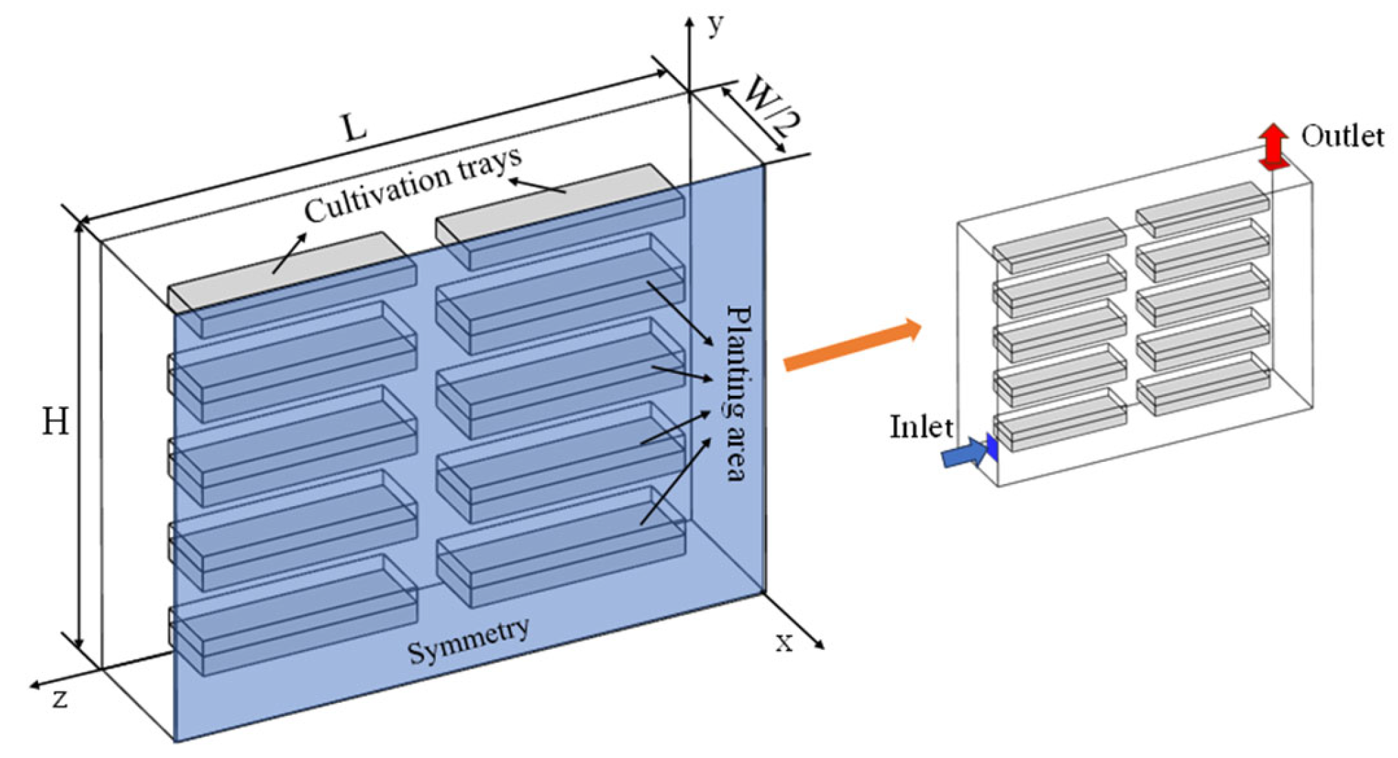
2.2. Geometrical Model

In this study, three-dimensional modeling of airflow and fluid heat transfer within a plant factory has been performed. The dimensions of the plant factory in the three-dimensional model are 4.4 m in length, 2.2 m in width, and 3.3 m in height. Four cultivation shelves with four layers of trays (tray number 1, 2, 3, and 4) are located inside the plant factory. The dimensions of the cultivation tray are 1.6 m in length, 0.5 m in width, and 0.15 m in height. The area of 0.12 m above the cultivation tray [25] is the crop planting area, which is of the same length and width as that of the cultivation tray and 0.12 m in height. The dimensions of the plant factory, the cultivation tray, as well as crop planting areas, are shown in

Table 2. Dimensions.

Domain	Dimensions: Length (L) × Width (W) × Height (H)
Room	4.4 × 2.2 × 3.3 m3
Cultivations	1.6 × 0.5 × 0.15 m3
Plant areas	1.6 × 0.5 × 0.12 m3

. In this research, it is assumed that both sides of the cultivation shelf are symmetrical, and one-half of the room is chosen as the target area for the study. The computational domain model of the research objective is shown in Figure 1.

2.3. Analysis of Data Indicators: Uniformity Assessment

In previous studies, it has been shown that airflow rate, temperature, and relative humidity above the crop canopy all play an important role in crop growth, which directly affects crop production quality and yield [10,17,50]. In this research, the objective uniformity parameter (OU) is used to evaluate the uniformity of airflow velocity distribution over the crop. The relative standard deviation (RSD) is employed to evaluate the uniformity of temperature and relative humidity. Relative standard deviation RSD is defined as the ratio of the standard deviation (SD) to the mean. The smaller the RSD, the lower the variance and higher the uniformity of the evaluated variables. The objective uniformity parameter [28] is defined by the following:

$$OU=\left(1-{\displaystyle \frac{S_U}{2U_0}}\right)\times 100\%$$

(12)

$$S_U=\sqrt{{\displaystyle \frac{1}{N-1}}{\sum }_{k=1}^N{\left(U_k-U_0\right)}^2}$$

(13)

where S_U is the standard deviation of the flow distribution within the plant factory relative to the target velocity. U_k and N are the average air velocity (m·s⁻¹) at the upper surface of the crop canopy of the k-th cultivation tray and the number of cultivation trays in the room, respectively. U₀ is the air velocity (m·s⁻¹) suitable for crop growth and it is taken as 0.4 m·s⁻¹ in this study, and the value of this velocity is considered to facilitate photosynthesis in crops [51].

The uniformity of air temperature and relative humidity distribution is assessed using the relative standard deviation (RSD), which is calculated as the ratio of the standard deviation to the mean. A smaller RSD indicates higher uniformity. Mathematically, it can be defined as follows:

$${RSD}_T={\displaystyle \frac{\sqrt{\frac{1}{N-1}{\sum }_{k=1}^N{\left(T_k-\overline{T}\right)}^2}}{\overline{T}}}\times 100\%$$

(14)

$${RSD}_{\mathit{RH}}={\displaystyle \frac{\sqrt{\frac{1}{N-1}{\sum }_{k=1}^N{\left({RH}_k-\overline{RH}\right)}^2}}{\overline{RH}}}\times 100\%$$

(15)

where RSD_T and RSD_RH are the relative standard deviation (%) of air temperature and relative humidity above the crop, respectively. T_k and RH_k represent the average air temperature (K) and relative humidity (%) above the kth cultivation tray crop, and $\overline{\mathrm{T}}$ and $\overline{\mathrm{R}\mathrm{H}}$ represent the overall average temperature (K) and average relative humidity (%) of the air above all crop areas, respectively.

In order to assess the overall impact of the uniformity of velocity, temperature, and relative humidity distribution on the system (cases with different planting density and ACH), the effective factor θ was used as an evaluation index. It is defined as follows:

$$\theta ={\displaystyle \frac{OU\frac{\overline{RH}}{{RH}_{\mathrm{Inlet}}}·\left(1-\frac{{RSD}_{\mathrm{T}}}{100}\right)·\left(1-\frac{{RSD}_{\mathrm{RH}}}{100}\right)}{\frac{∆p·ACH}{∆p_{\mathrm{Base}}{ACH}_{\mathrm{Base}}}·\frac{\overline{T}}{T_{\mathrm{Inlet}}}}}$$

(16)

where ∆p represents the magnitude of pressure change and ∆p_Base represents the magnitude of pressure change for the reference case.

3. Description of the Study Case and Boundary Conditions

3.1. Description of the Study Case

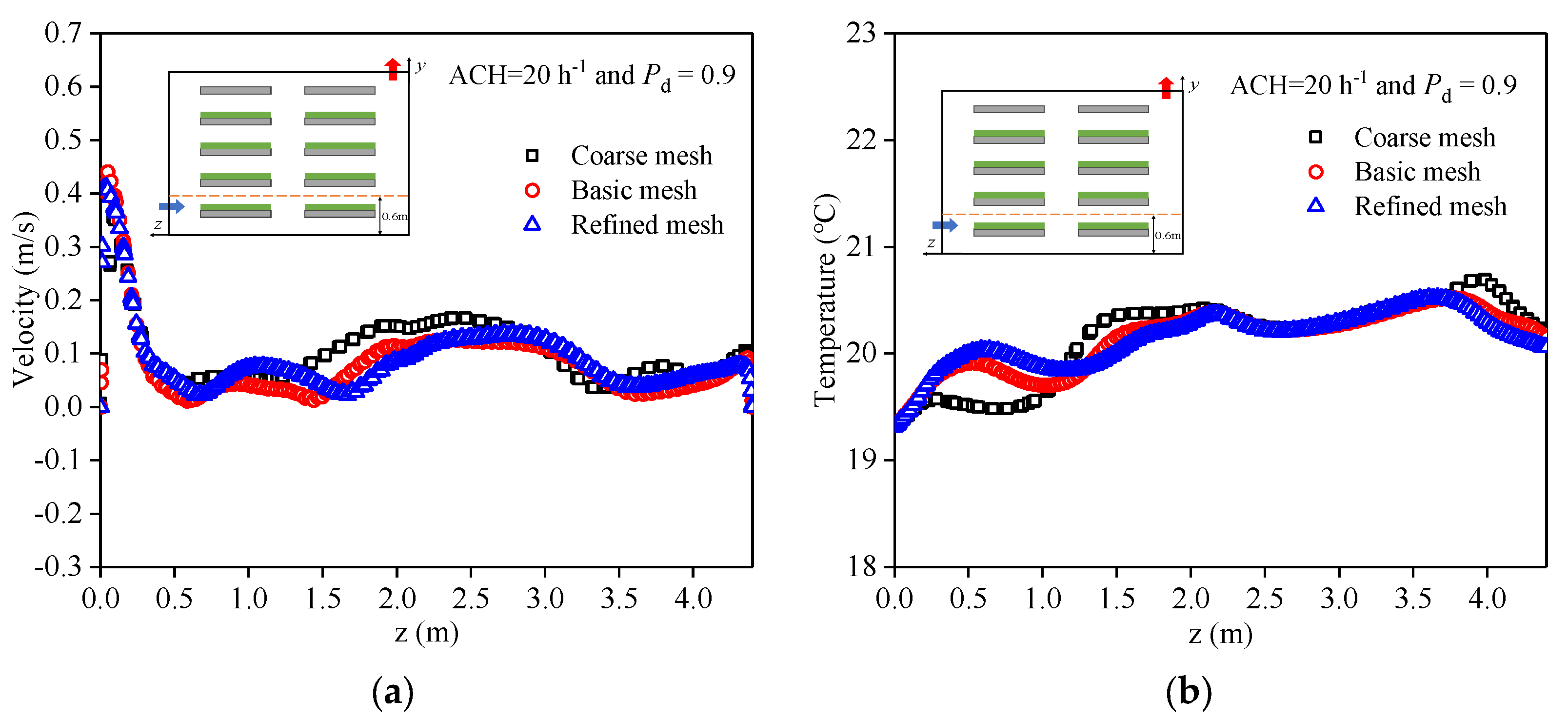
In this study, the effects of different crop planting density and the air change rate for indoor ventilation on the climatic uniformity of air velocity, temperature and relative humidity above the crop canopy in the plant factory are considered. It is assumed that the volume occupied by each plant is uniform and that the volume of space occupied by each cultivation area is constant. Therefore, according to the definition of porosity, the change in porosity of the crop cultivation area is employed to indicate the change in density of the cultivation area; the larger the ϕ, the smaller the space occupied by the crop, which means the lower the planting density. The planting density of the crop is defined as follows:

$$P_{\mathrm{d}}=1-\varphi$$

(17)

where P_d denotes the planting density of the crop in the cultivation zone.

In the study, the uniformity of air velocity, temperature and relative humidity in the crop canopy is assessed for five different crop density cases (P_d = 0.1, 0.3, 0.5, 0.7, 0.9). To illustrate the effect of variations in planting density on airflow, crop resistance was calculated using Equation (4), where C_F is set to 0.25 m⁻¹ [39] and the mean diameter d_p is taken as 0.11 m [25]. The permeability K_p is determined from the porosity ϕ. In addition, a schematic diagram illustrating the variation in planting density within the crop area can be found in Figure 2. In the study, the outlet boundary condition of the computational domain is defined as the pressure-outlet. The inlet boundary of the computational domain is set to the velocity-inlet. Considering that the plant factory enclosure has high thermal insulation properties, the heat absorption and dissipation from the surrounding walls are not considered and the heat energy released by light to the surroundings through radiation was ignored in the study [11,52]. Therefore, the surrounding walls are set as adiabatic boundaries. All boundary conditions and materials are listed in

Table 3. Boundary conditions and materials.

Parameters	Boundary Conditions
Inlet	ACH = 20, 40, 60, 80, 100 h−1 (fluid: air and water vapor temperature: 19 °C, relative humidity: 80%)
Outlet	Pressure outlet (zero pressure)
LED lights	Wall (material: aluminum; thermal: isothermal wall and temperature = 40 °C [25])
Planting areas	Porous media (material: leaf, density: 1078 kg m−3, specific heat: 3100 J kg−1 K−1, thermal conductivity: 0.55 W m−1 K−1 [53])
Cultivation trays	Adiabatic wall (material: aluminum)
Walls of the farm	Adiabatic wall (material: aluminum)
$P_{\mathrm{d}}$	C1	C2	Inlet_ACH (h−1)
0.9	1.2 × 107	1735.6	20, 40, 60, 80, 100
0.7	2.7 × 105	259.8	20, 40, 60, 80, 100
0.5	2975.2	27.3	20, 40, 60, 80, 100
0.3	390.3	9.9	20, 40, 60, 80, 100
0.1	20.4	2.3	20, 40, 60, 80, 100

.

3.2. Mesh Analysis

In the study, the hexahedral type of mesh is applied to discretize the entire computational domain. Finer mesh sizes are used near LED light walls, crop area surfaces, and airflow inlet and outlet surfaces. To ensure that the numerical results are not affected by the size and number of mesh, the results are simulated for three cases where the number of mesh is 552,789 (Coarse mesh), 1,984,032 (Basic mesh), and 2,847,910 (Refined mesh). The variation in air velocity and temperature along the z-axis direction for y = 0.6 m and x = 0.55 m in the numerical model is compared in Figure 3. As shown in Figure 3, the difference between the velocity and temperature predictions of the refined and basic meshes is minimal. Therefore, in order to achieve an optimum between the accuracy of the simulation results and computational efficiency, the model mesh is chosen as the basic mesh in the following numerical simulation study.

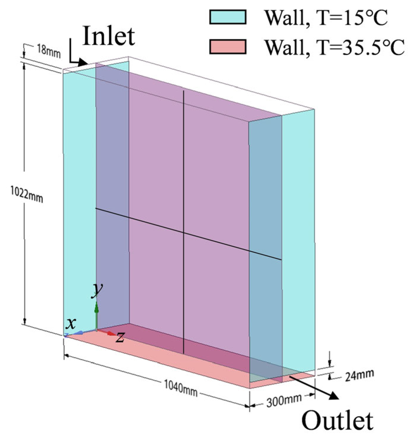
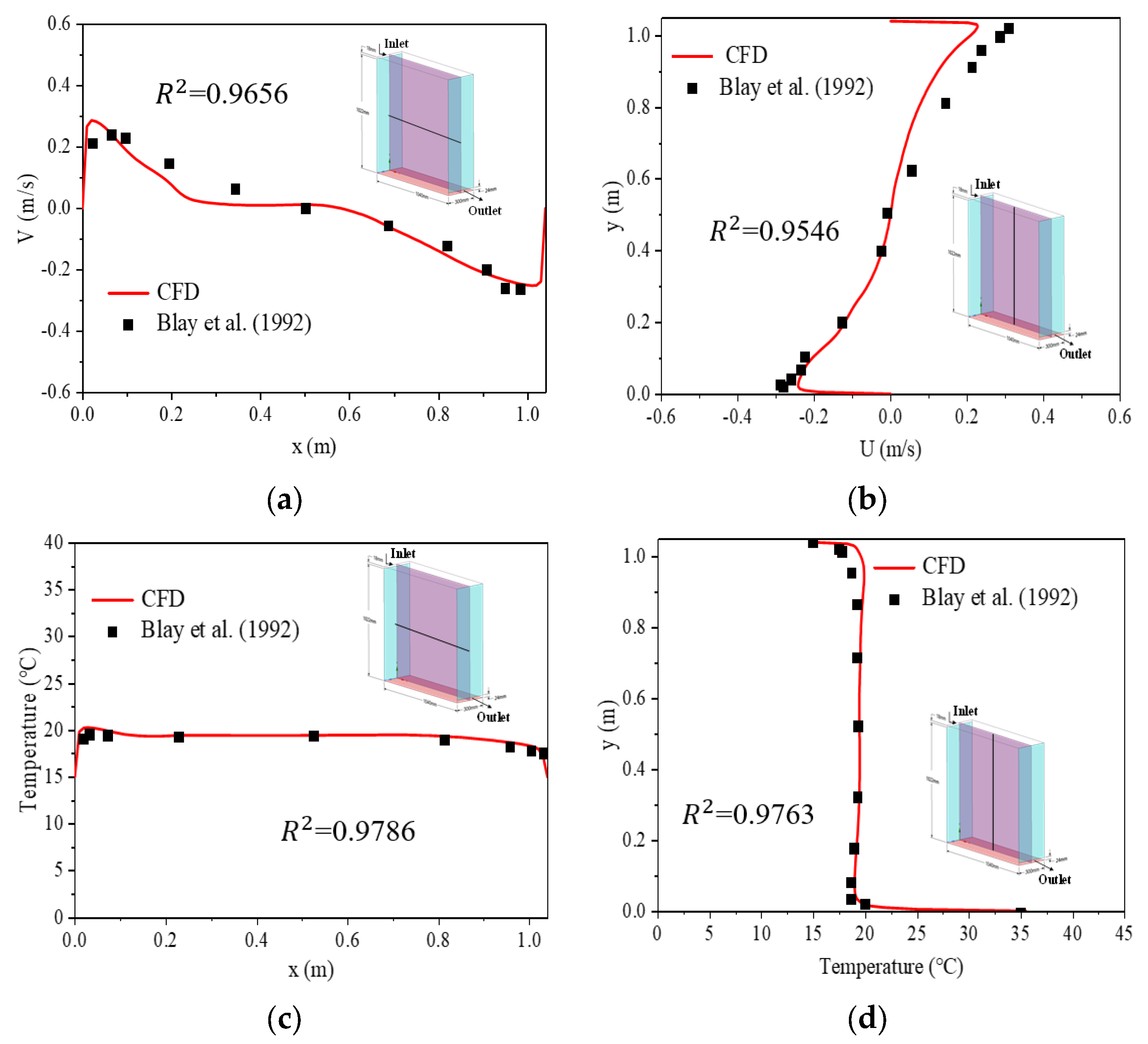
3.3. Model Validation

In this study, the experimental data from Blay et al. on non-isothermal mixed convection in a square-type ventilated box were employed for model validation [54]. An experiment was conducted in a cavity with dimensions of 1040 × 1040 × 700 mm³ (D × H × W), where an air inlet with a height of 18 mm was set on the wall on the width side and an outlet with a height of 24 mm was set at the bottom of the wall opposite to the inlet. The entire cavity was divided into three smaller cavities, including the measuring cavity in the center and the protective cavities on both sides, which are separated by transparent double glazing. The cavities on both sides were used to eliminate the influence of the surrounding thermal environment on the flow in the center measurement cavity. Moreover, the surrounding walls were maintained at a constant uniform wall temperature (15 °C) using a temperature-controlled water system, while the bottom wall was heated to 35.5 °C and maintained at a constant level. The inlet air temperature was controlled at 15 °C in the experiment, the inlet velocity was set to 0.57 m/s, and the turbulence intensity at the inlet was 6%. Time-averaged velocity and temperature measurements were performed when the experimental conditions reached a statistical steady state. The measurements from this experiment provide validation support for numerical calculations of the non-isothermal mixed flow and heat transfer of indoor air [55,56].

In order to validate the accuracy of the numerical model in predicting the experimental results, this study validates the turbulence model for non-isothermal convective airflow conditions using the experiments conducted by Blay et al. (1992) [54]. In this numerical model, the computational domain was specifically designed and meshed to focus on the central cavity where the measurements were performed in the experiment. The outer two cavities were not included in the model. The two side walls without inlets and outlets were designated as adiabatic walls to emulate the impact generated by the two side cavities, thereby circumventing the influence of the external environment on the flow pattern within the central cavity (Figure 4). In the model construction, a tetrahedral mesh was employed to discretize the computational domain. To enhance the accuracy of predicting velocity gradients and convective heat transfer, a finer mesh was employed on the surfaces of the inlet, outlet, and the bottom hot wall within the computational domain. The distributions of vertical velocity components (V) and horizontal velocity components (U) along the horizontal center line (y/L = 0.5) and vertical center line (x/L = 0.5), as well as the air temperature, are compared between the numerical model and the experimental measurements conducted by Blay et al. [54]. From Figure 5, it is evident that the numerical model accurately predicted both the velocity and temperature distributions. This indicated that the existing numerical model was reliable and could ensure the accuracy of subsequent simulation studies.

4. Results and Discussion

This section discusses the results of numerical simulations of air movement and transport of heat and humidity above indoor crops in the plant factory for five crop area planting density (P_d) and five air change rates (ACH). The objective uniformity parameter (OU), relative standard deviation of temperature (RSD_T), and relative standard deviation of relative humidity (RSD_RH) are used to assess the air velocity, temperature, and relative humidity uniformity above the crop in the plant factory, respectively.

4.1. Uniformity of Air Velocity Distribution

The air velocity above the crop in the plant factory is one of the key factors affecting the growth rate of the crop. Relevant research has shown that air movement could enhance the exchange of substances between air and plants and enhance photosynthesis when the horizontal velocity of the air above the plant is between 0.3 m·s⁻¹ and 0.5 m·s⁻¹ [51]. In plant factory farming systems, the obstruction of indoor airflow by the cultivation trays and the crop itself leads to a decrease in air velocity and increasing non-uniformity of air velocity distribution above the crop planting areas. Hence, it is crucial to investigate the impact of the air change rate (ACH) of an indoor ventilation system and the planting density in crop areas on indoor airflow patterns. The objective uniformity parameter (OU) is utilized to evaluate the uniformity of canopy air velocity distribution in indoor plant cultivation areas. As OU indicates the deviation of the air velocity above the crop from the suitable velocity for each cultivation tray, a higher OU value signifies a more uniform air velocity distribution above the crop.

Figure 6 presents a comprehensive overview of the variations in the overall OU with ACH above the crop across all five different cultivation densities. It can be observed that, in general, OU is increasing with increasing ACH values in the plant factory and the uniformity of the air velocity distribution over the crop varies between 48% and 76%. (Figure 6). The velocity distribution for the case of P_d = 0.5 in the indoor crop area is chosen as the basis for analyzing the variation in indoor air velocity distribution with increasing ACH. This particular case, at P_d = 0.5 in the crop area, effectively represents the overall trend of OU values with increasing ACH for each planting density (Figure 6). As depicted in Figure 7, it is evident that the overall indoor air velocity experiences a significant increase with higher ACH values in the room. Furthermore, the indoor mixed flow is enhanced as the ACH increases. Additionally, the deviation of the air velocity from the optimal air velocity (U₀ = 0.4 m·s⁻¹) above each cultivation tray decreases. This ultimately contributes to an increase in OU in the room (Figure 6). As the ACH increased, the OU of indoor did not consistently increase. Specifically, in the case of indoor crop area with P_d = 0.1, the OU achieved a maximum value of 72.6% at ACH = 80 h⁻¹ and then decreased as the ACH further increased. This is due to the fact that, as the ACH increases, the average velocity of the airflow over the crop area of the lowest indoor cultivation tray is much greater than U₀ = 0.4 m·s⁻¹, which leads to a lower overall indoor OU value. It can be observed that smaller P_d values result in larger OU values in the indoor under the same ACH conditions. To further analyze this phenomenon, let us discuss the case of ACH = 80 h⁻¹. Figure 8 depicts the two-dimensional velocity distributions of the five P_d values of the crop in the x-z plane above the cultivation tray. It is evident that, in the cases where P_d > 0.5 in the crop area, the higher planting density leads to increased resistance to airflow, resulting in lower air velocities above each cultivated tray. Consequently, the overall increase in OU above the crop area is less pronounced when ACH is increased in these cases (Figure 6). In contrast, when P_d ≤ 0.5 in the crop area, the crop exhibits less resistance to airflow, causing the air velocity above the crop to increase significantly as P_d decreases (Figure 8). This indicates that lower planting densities result in a substantial increase in the U₀ value with increasing ACH. Furthermore, at the same ACH, the OU value is larger at smaller planting density (P_d ≤ 0.5) compared to larger planting density (P_d > 0.5). It is apparent that, as P_d decreases in the crop area, particularly when P_d < 0.5, the air velocity above the bottom cultivation tray increases significantly, surpassing the optimal air velocity U₀ = 0.4 m·s⁻¹. This phenomenon is attributed to the positioning of the air inlet at the bottom. Consequently, this is also reflected in the decrease in OU values in the indoor scenario with P_d = 0.1 and ACH = 100 h⁻¹. In summary, a smaller value of P_d in the crop results in a higher OU value in the room. Specifically, when ACH is further increased (ACH > 80 h⁻¹), the average air velocity above the crop area of the lowest cultivation tray becomes excessively high, leading to a decrease in the overall OU of the indoor in the case of crop P_d = 0.1.

Furthermore, it can be observed that the air velocity above the crop in the cultivation tray near the outlet side is higher compared to the cultivation tray on the inlet side. This discrepancy is attributed to the heat generated by the LED lamps, which results in a higher air temperature at the outlet compared to the air temperature at the inlet. As a result of the thermal buoyancy force induced by the heat dissipation of the LED lamps in the room, the air with the higher temperature near the exit side tends to flow upwards. Therefore, based on the variation in OU with ACH depicted in Figure 6, it can be concluded that increasing ACH or decreasing P_d generally results in higher OU values. However, it should be noted that the combination of higher ACH and lower P_d does not necessarily imply greater OU values, as observed in the case of P_d = 0.1 and ACH = 100 h⁻¹. This occurs because, when the ACH is too high, the excessive air velocity at the inlet of the indoor ventilation system causes the air velocity above the cultivated tray crop near the inlet side to become too high. As a result, the air velocity deviates significantly from the optimum velocity (U₀), leading to a decrease in the overall OU value of the room. Hence, in situations where the planting density of the indoor cultivation tray crop area is high, increasing the ACH value can enhance the overall uniformity of the airflow rate above the indoor crop area. Conversely, when the planting density of the indoor cultivation tray crop area is low, a smaller ACH value can be utilized, potentially reducing energy consumption related to the ventilation system while still ensuring improved airflow uniformity over the crop area.

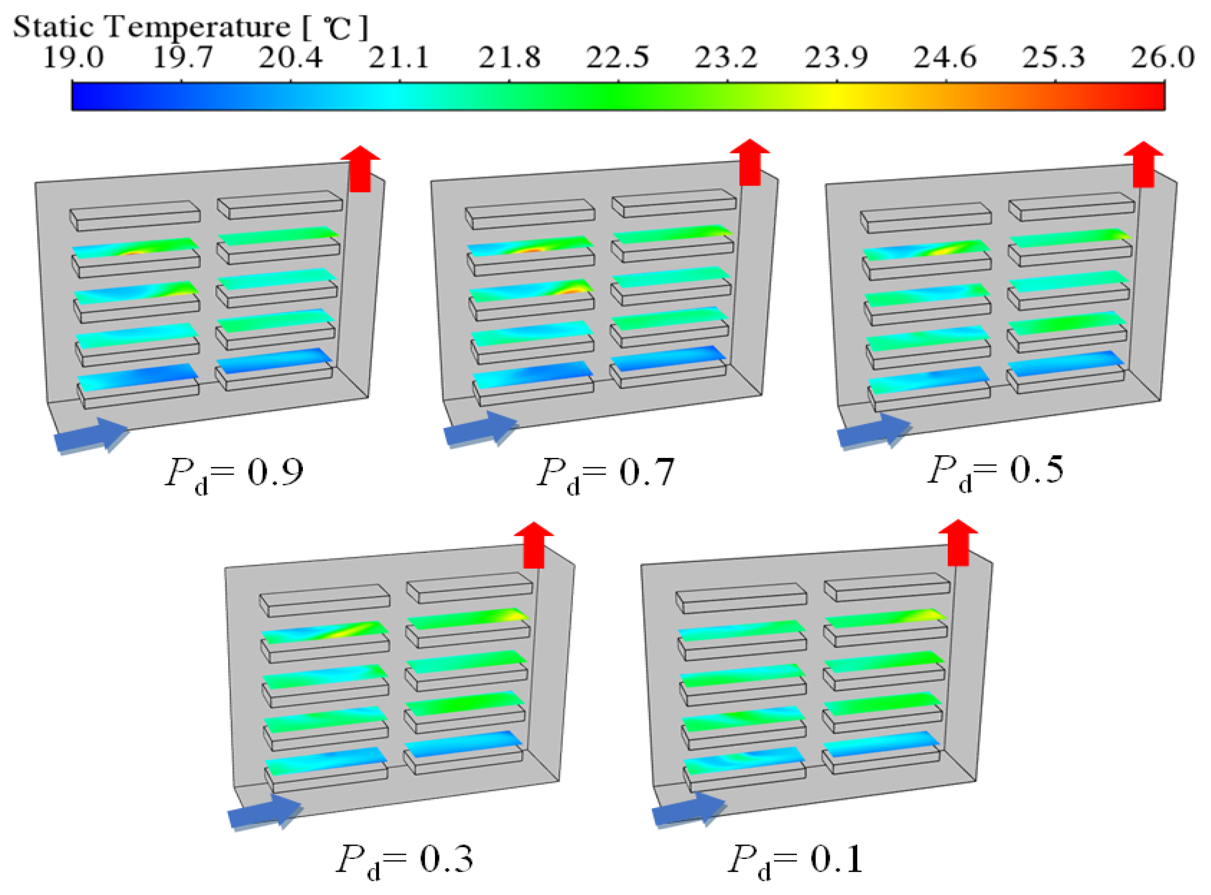
4.2. Air Temperature Distribution and Relative Temperature Deviation

Air temperature is vital for the process of plant photosynthesis and is a crucial parameter that needs to be controlled and monitored in a plant factory. The temperature of the airflow above the crop has a direct impact on the relative humidity (RH) of the airflow and consequently affects the growth and development of the plants [15]. In subsequent analyses, the air temperature distribution above the crops in different crop areas will be investigated on the basis of P_d and ACH. In addition, the uniformity of temperature distribution will be assessed by analyzing the relative standard deviation of temperature.

Figure 9 depicts the average temperature above the crop in each layer of the cultivation tray at various planting density (P_d) as a function of ACH. From Figure 9, the following observations can be made: (1) in the cases with crop area P_d > 0.5 and ACH ≤ 60 h⁻¹, the average air temperature above the crops in the upper cultivation tray (layer 3 and 4 of the cultivation tray) is consistently higher than that in the lower cultivation tray (layer 1 and 2 of the cultivation tray). In the case of ACH > 60 h⁻¹, there is a phenomenon where the air temperature above the crop area in layer 2 of the cultivation trays is higher than that in layer 3. (2) In the case of crop area P_d ≤ 0.5, higher air temperatures above the crop area in layer 2 of the cultivation tray than in layer 3 already occur in the case of ACH = 60 h⁻¹. (3) As the ACH increased, the air temperature above the crops in each layer decreased. Specifically, in the case of a crop area with P_d = 0.1, the air temperatures above the crops in layers 1, 2, and 3 of the cultivation trays demonstrated a clear tendency to increase and then decrease.

To further understand the underlying causes of the aforementioned phenomenon, an analysis was conducted on the distribution of air temperature above the crops in the cultivation tray. Figure 10 presents the two-dimensional temperature distribution above the crops for a crop area with P_d = 0.3, with variations in ACH. It is evident that, when ACH ≤ 60 h⁻¹, the room exhibits a noticeable temperature stratification due to the combined impact of the inlet airflow and the thermal effect of the LED lamps. Consequently, the average temperature of the airflow above the crops in the upper cultivation tray (layer 3 and 4 of the cultivation tray) consistently surpasses that in the lower cultivation tray (layer 1 and 2 of the cultivation tray). When ACH > 60 h⁻¹, the effect of thermal buoyancy on the indoor flow structure is weakened due to the increase in inlet air velocity, and the inlet airflow dominates the indoor airflow pattern. The mixed flow of inlet air and indoor air affected the lower layer above the crop, resulting in lower airflow temperatures above the crop in layer 3 of the cultivation tray than in layer 2 of the cultivation tray. Similarly, air velocity above the crop increases significantly due to lower planting density (P_d < 0.5) and weaker obstruction of airflow by the crop (Figure 8).

To further analyze the distribution of air temperature above all crop areas at various planting density, the two-dimensional temperature distribution above the crop in five different P_d is presented in Figure 11. These distributions are obtained under a constant ACH of 60 h⁻¹. It can be observed that the air temperature above the lower cultivation tray is lower than the air temperature above the upper cultivation tray. Additionally, the air temperature above the crop in the upper cultivation tray is greater in the case of lower P_d than in the case of higher P_d. As depicted in Figure 8, the air velocity above the crops in the upper cultivation tray is higher when the P_d of the crop area is lower compared to when it is higher. This can be attributed to the lower resistance to flow within the room at lower P_d, which facilitates a stronger mixing flow within the heated air.

The uniformity of air temperature distribution above the crops plays a crucial role in promoting optimal crop growth. Figure 12 illustrates the variation in the overall RSD_T of the air temperature above the crops at all five planting densities at different ACH. It can be observed that the highest RSD_T values occur at ACH = 20 h⁻¹ for all planting densities. This is because, in cases with lower ACH where the indoor air is primarily influenced by thermal buoyancy, there is a tendency for temperature stratification along the height. As the ACH increases, the RSD_T decreases for all planting density cases. This is because the inlet of low-temperature air increases, leading to a stronger mixing flow indoors (Figure 13). Consequently, the influence of thermal buoyancy on the indoor airflow gradually diminishes, resulting in a more uniform air temperature distribution above the crop. Moreover, as the ACH increased (in cases where ACH < 60 h⁻¹), the RSD_T decreased significantly in all cases with P_d, though it showed a weaker decrease in cases where ACH > 60 h⁻¹. Meanwhile, the disparity between the RSD_T of each P_d decreased with increasing ACH. This can be attributed to the fact that, when the ACH exceeded 60 h⁻¹, although there is a gradual improvement in the mixed airflow within the room, it did not have a significant impact on reducing the temperature differences above the crops in each layer of the cultivation trays. Consequently, the changes in RSD_T at each P_d became insignificant. From the temperature distribution analysis in the room with different P_d and ACH, it can be observed that increasing ACH and decreasing P_d appropriately can enhance the uniformity of temperature distribution. However, it is noteworthy that further increasing ACH (in the case of ACH > 60 h⁻¹) and decreasing P_d does not result in a significant decrease in the RSD_T. Additionally, it is important to note that significant thermal stratification occurs at lower ACH values, leading to higher RSD_T values. On the other hand, increasing the ACH results in higher energy consumption by the ventilation system.

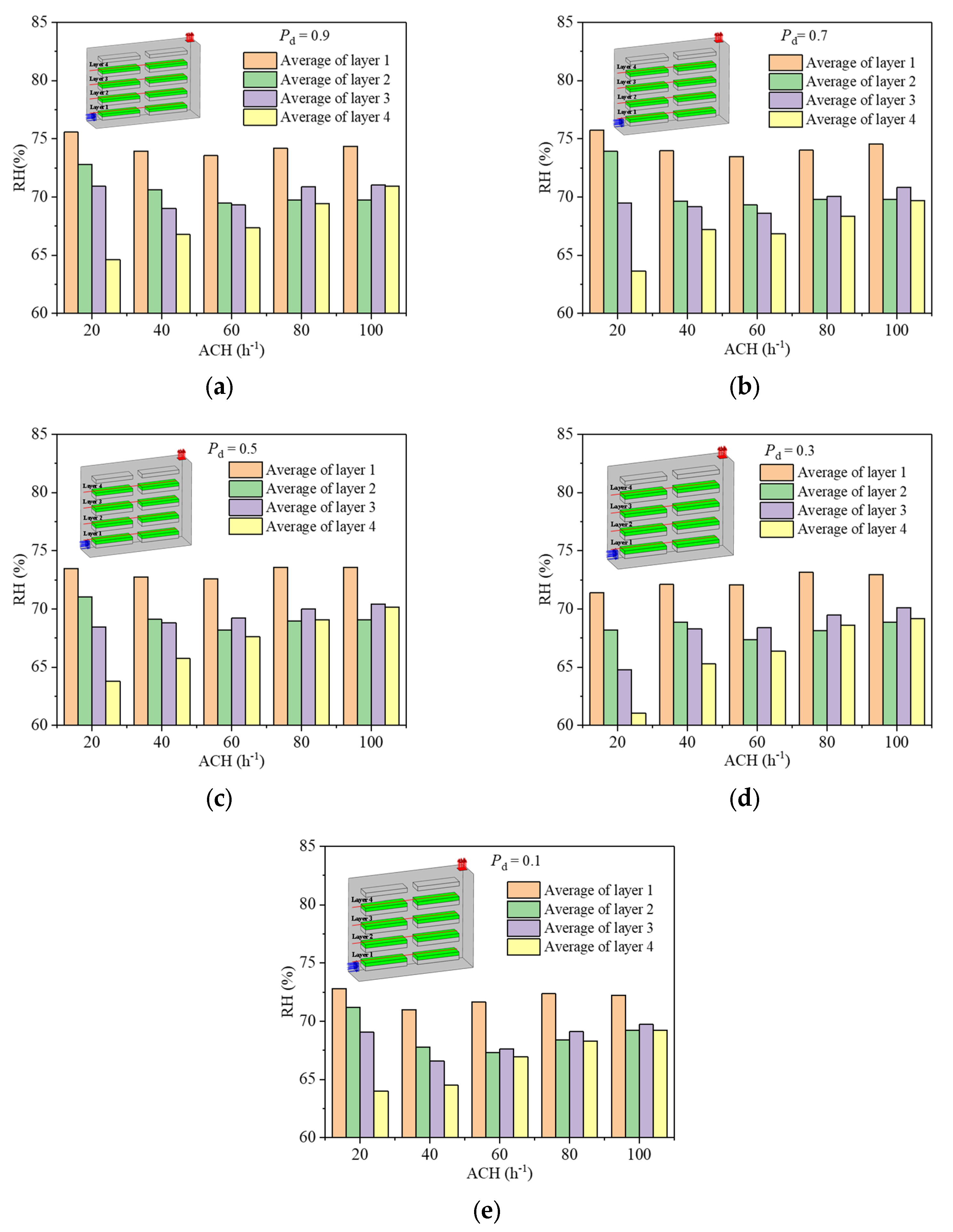
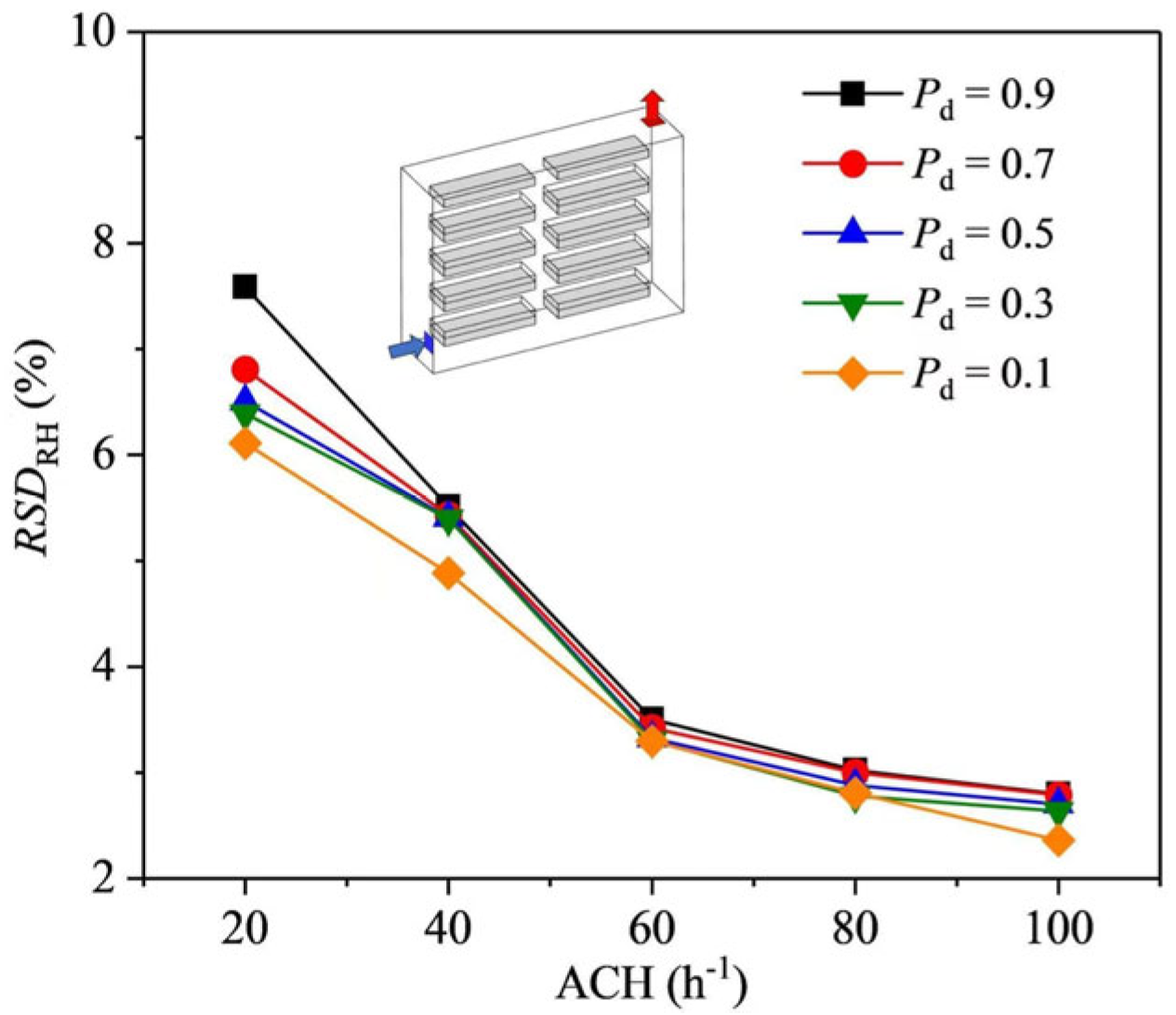
4.3. Relative Air Humidity and Relative Deviation of Relative Humidity

The relative humidity (RH) of the air represents the level of partial pressure of water vapor in the indoor air, which has a significant effect on photosynthesis as well as transpiration in plants. According to relevant studies, it is recommended to maintain the air relative humidity between 50% and 70% for optimal growth of green leafy vegetables [57]. Excessively high relative humidity of the air can impede plant transpiration and increase the risk of pathogenic bacterial infections, while excessively low relative humidity of the air can result in leaf burn [15]. Thus, it is essential to analyze the variations in indoor relative humidity distribution.

Figure 14 and Figure 15 depict average relative humidity (RH) and relative standard deviation of relative humidity (RSD_RH) values above the crop in each layer of cultivation trays at different air change rate (ACH) for the five P_d as concerned. From Figure 14, it can be observed that, in the cases with P_d > 0.5 and ACH ≤ 60 h⁻¹, relative humidity of the air above the crop area of each layer of cultivation trays decreases with the increase in the height of cultivation trays, while in the cases with ACH > 60 h⁻¹, it appears that average relative humidity of the air above the crop area of the third layer cultivation trays is greater than that of the secondary layer cultivation trays. In the instances where simultaneously satisfying P_d ≤ 0.5 and ACH ≤ 40 h⁻¹, relative humidity above the crop area in each layer of cultivation trays decreases as the height of the cultivation trays promotes. However, in the case of ACH = 60 h-1, volume-averaged relative humidity above the crop area in the third layer cultivation trays is higher than that in the secondary layer cultivation trays. In cases where P_d > 0.5 and ACH > 60 h⁻¹, average relative humidity above the crop area in the third layer cultivation tray was higher than that in the secondary layer one. Figure 15 shows the overall RSD_RH above the crop at five planting density at different ACH scenarios. It can be found that RSD_RH decays for all P_d cases as ACH increases. Overall, relative humidity (RH) levels above the crops in each layer of the cultivation tray are generally falling within the appropriate range (air relative humidity between 50% and 70%) for all five P_d and different ACH. However, it is worth noting that the air above the crop area of the first layer cultivation tray tends to promote RH levels.

4.4. Overall Effective Factor

In this research, each of the uniformity indicators discussed is affected by the planting density of the crop (P_d) and the air change rate (ACH). In order to comprehensively analyze the environmental parameters including air velocity, temperature, relative humidity, and various uniformity indices, a comprehensive assessment of the validity of different planting density (P_d) and air change rate (ACH) has been conducted using the validity factor θ in Equation (16). First, a discussion case of P_d = 0.9 is presented in this research. Figure 16 illustrates the profiles of θ for five different crop planting density (P_d) with varying ACH values. The figure demonstrates that, as ACH increases, the majority of θ values for all five P_d conditions tend to increase, indicating a positive correlation between ACH and θ. Additionally, it is observed that lower crop planting density generally exhibit higher θ values. However, it is worth noting that, for the case of P_d = 0.1 and ACH > 60 h⁻¹, the θ values are lower compared to the case of P_d = 0.3. Even when ACH is set to 100 h⁻¹, the θ values for P_d = 0.1 are lower compared to P_d = 0.5. Since OU plays a dominant role in determining the θ values, the trend of θ is similar to that of OU, as evident from Figure 6 and Figure 16. From the findings discussed above, it can be observed that, while increasing ACH and decreasing P_d generally leads to higher overall θ values in the room, there are cases (e.g., ACH = 100 h⁻¹ and P_d = 0.1) where high ACH and low P_d result in a decrease in θ. It is important to note that increasing ACH in the room will also lead to higher energy consumption. Furthermore, it is observed that, in the case of P_d < 0.3, reducing the crop planting density does not significantly improve the θ value. This is because the difference between the RSD_T and RSD_RH values under each P_d condition is not substantial. It is worth noting that reducing the planting density too much may result in lower crop yield. To enhance the overall θ, it is recommended to increase the indoor ACH and lower the crop planting density (P_d) to an appropriate extent. However, it is crucial to select an optimal combination of ACH and P_d that strikes a balance between energy consumption and crop yield.

5. Conclusions

In this research, the computational fluid dynamics (CFD) model has been developed to investigate heat/moisture transfer and fluid flow in the agriculture plant factory. The CFD model has been used to analyze and understand the distribution characteristics of airflow, temperature, and relative humidity. The effects of planting density (P_d) and air change rate (ACH) on the air velocity, temperature, relative humidity distribution, and uniformity above the crop in a plant factory, have been investigated with an accompanying comprehensive analysis and discussion. The purpose of the present work was to understand how P_d and ACH influence the airflow patterns and microclimate conditions within the plant factory, particularly within the region of crop plants. The following main conclusions were obtained:

After carefully varying ACH and crop planting density (P_d) in CFD simulation cases, uniformity of air velocity distribution above the crop was confirmed in the range between 48% and 76%.

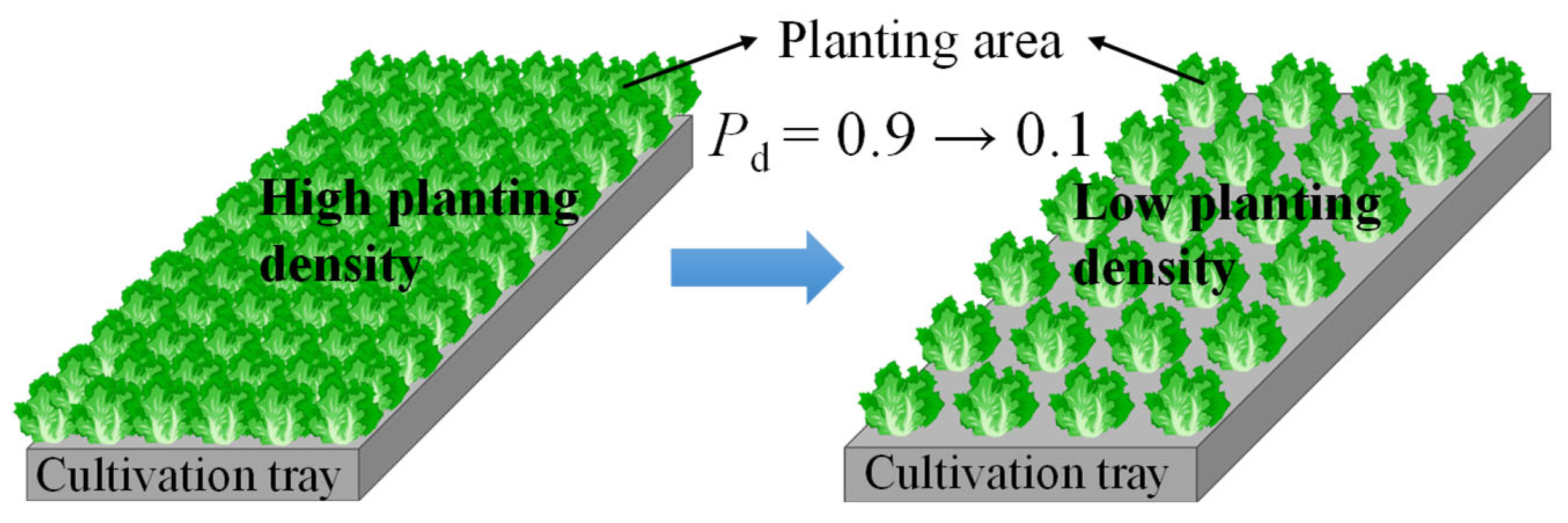
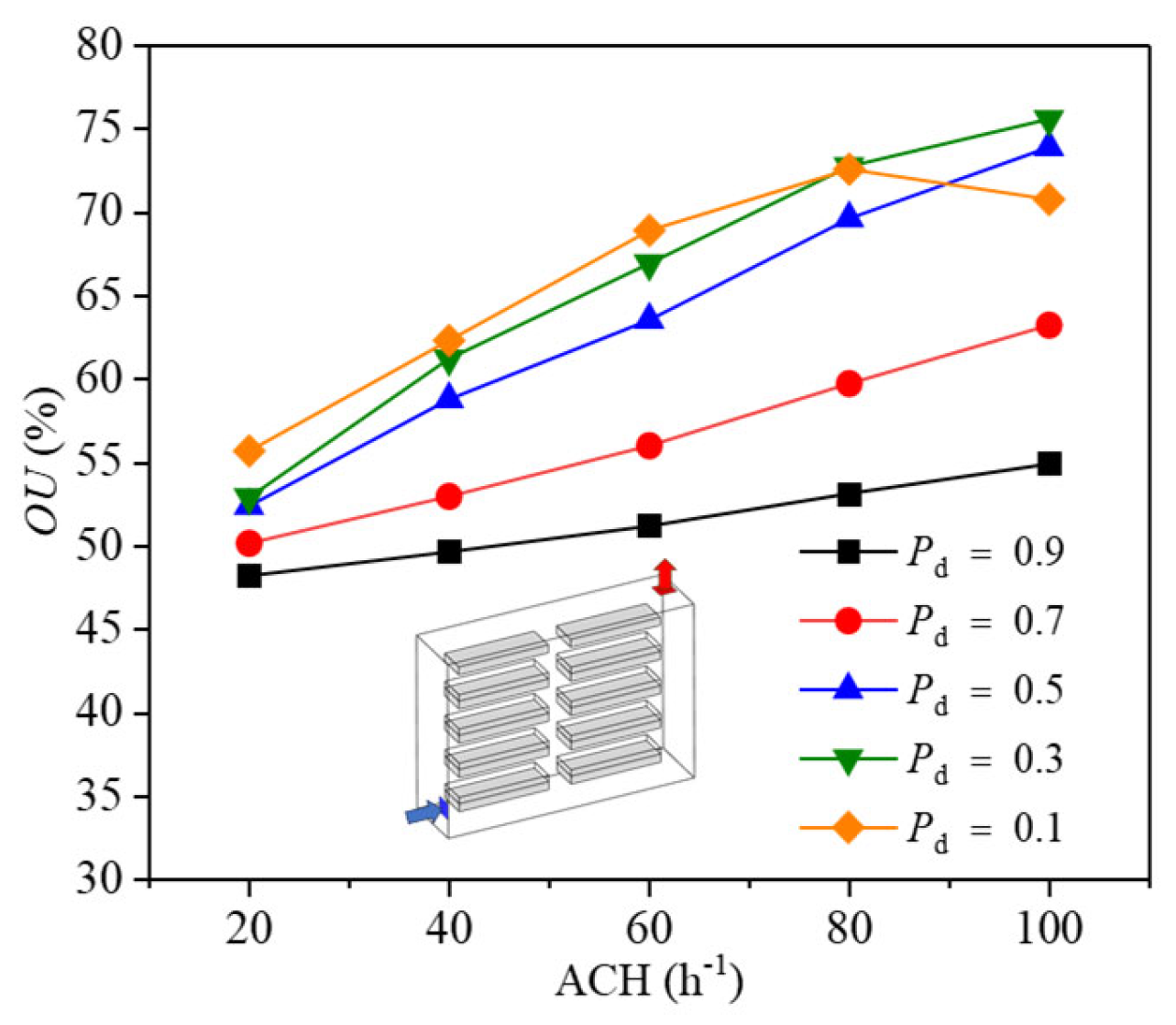
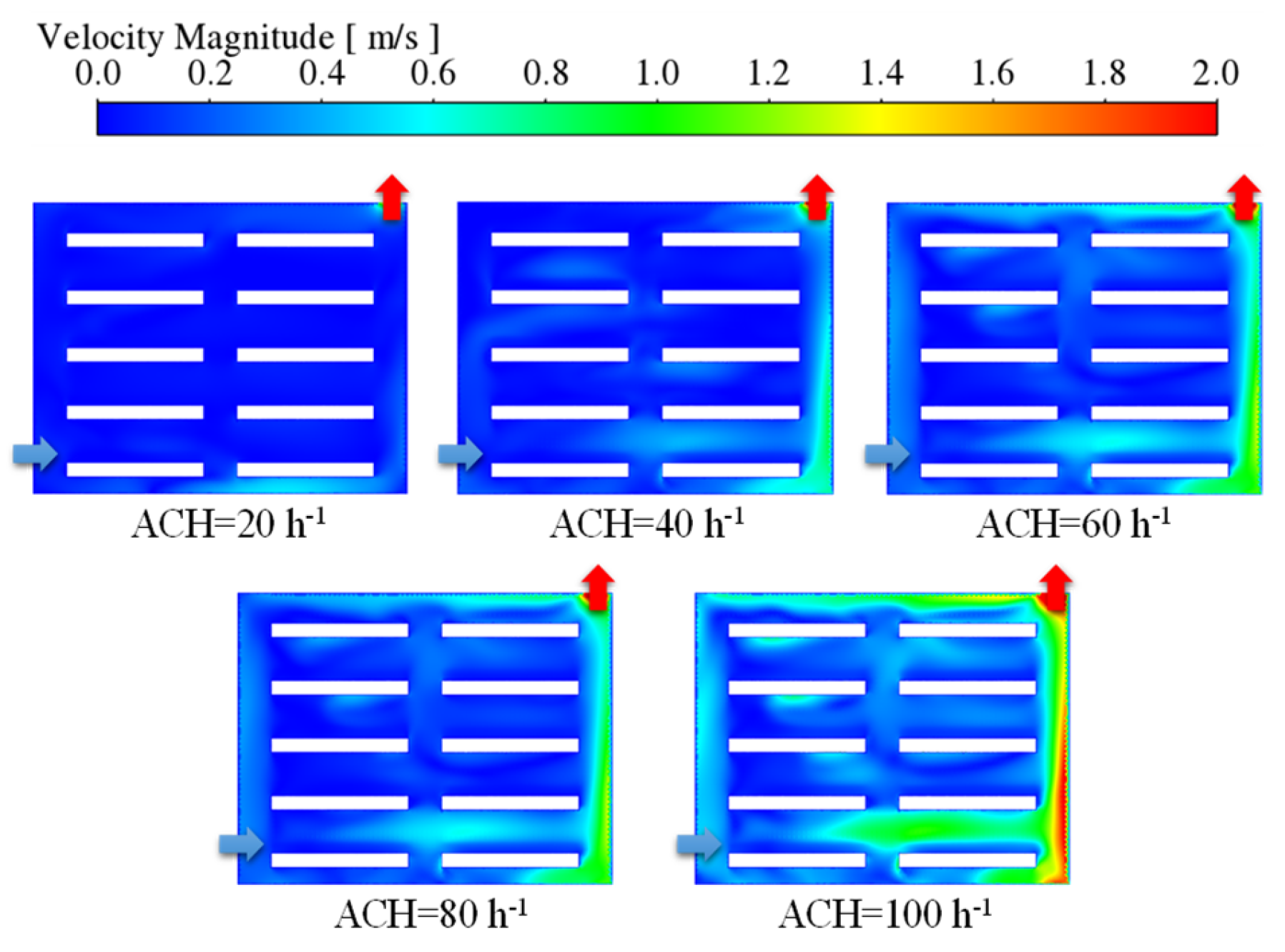
• In the cases of identical ACH, airflow velocity above the crop in areas with low planting density becomes higher than that with high planting density. This was essentially due to the fact that lower resistance of the sparse planting crops was presented to the airflow fields.
• Smaller planting density (P_d) and larger ACH promote a greater uniformity of air velocity distribution. However, it is important to note that excessively small planting density (P_d) of crop area and overly large ACH do not necessarily result in a more favorable airflow distribution uniformity. This is because a very small planting density (P_d) of crop area and an extremely large ACH could lead to excessively high air velocity above the crops in the bottom cultivation trays. As a result, this could expand the deviation from the optimal air velocity (U₀ = 0.4m·s⁻¹) and consequently reduce the value of OU in the entire room.
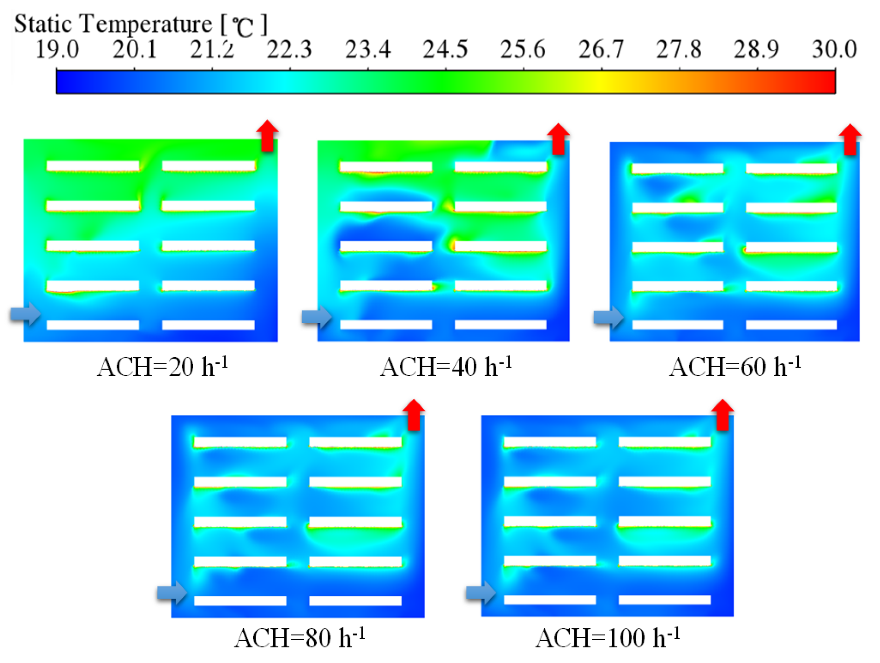
• Air temperature and relative humidity above the crop area of each cultivation tray layer are significantly influenced by different categories of ACH and planting density (P_d). In the case of a smaller ACH, thermal buoyancy generated by the indoor LED lights has a more pronounced or sensible effect, resulting in significant thermal (temperature) stratification in the room-space. As a result, the relative deviation of temperature (RSD_T) in the room becomes higher, which in turn leads to a higher relative deviation of relative humidity (RSD_RH).
• As ACH increases, both the relative deviation of temperature (RSD_T) and relative deviation of relative humidity (RSD_RH) of the air above the crop decay in any discussed cases of crop area planting density (P_d). Moreover, smaller planting density (P_d) values result in smaller values of RSD_T compared to RSD_RH for the air above the crop.
• It should be especially noted that excessive increment in ACH and decay in P_d did not have a significant effect on θ, which was influenced by a combination of OU, RSD_T, and RSD_RH. Therefore, a more appropriate combination of ACH and P_d could be needed in the design to balance energy use and crop yield. To enhance the uniformity of air velocity, temperature, and relative humidity above the crops, joint effects of crop planting density and ACH could be further optimized.

This research has uncovered the roles of crop planting density and air change rate on the microclimate above crops in plant factory. These findings could serve as a valuable reference for designing modern agricultural systems with the aim of boosting the productivity of crop production in plant factories.

6. Limitations and Further Research

• In the actual production of plant factories, changes in the external climate environment (such as changes in temperature and humidity, changes in solar radiation, alternation of day and night, and seasonal changes.) have a significant impact on the climate environment inside the plant factory. This study mainly considers the ventilation and cooling of plant factories under stable external environment. However, the impact of changes in the external environment was not considered.
• In the actual operation process, most plant factories exist in large-scale multi-building forms. The climate environment in the plant factory is more complex. This paper mainly studies the climate environment inside a single-building plant factory and ignores the effects of soil evaporation and heat storage. The influence of the above factors can be considered in future research.

References

1. Pandey, B.; Seto, K.C. Urbanization and agricultural land loss in India: Comparing satellite estimates with census data. J. Environ. Manag. 2015, 148, 53–66. [Google Scholar]
2. Namara, R.E.; Hanjra, M.A.; Castillo, G.E.; Ravnborg, H.M.; Smith, L.; Van Koppen, B. Agricultural water management and poverty linkages. Agric. Water Manag. 2010, 97, 520–527. [Google Scholar] [CrossRef]
3. Piao, S.; Ciais, P.; Huang, Y.; Shen, Z.; Peng, S.; Li, J.; Zhou, L.; Liu, H.; Ma, Y.; Ding, Y. The impacts of climate change on water resources and agriculture in China. Nature 2010, 467, 43–51. [Google Scholar] [CrossRef]
4. Godfray, H.C.J.; Beddington, J.R.; Crute, I.R.; Haddad, L.; Lawrence, D.; Muir, J.F.; Pretty, J.; Robinson, S.; Thomas, S.M.; Toulmin, C. Food security: The challenge of feeding 9 billion people. Science 2010, 327, 812–818. [Google Scholar] [CrossRef]
5. Alexandratos, N.; Bruinsma, J. World Agriculture Towards 2030/2050: The 2012 Revision; FAO: Rome, Italy, 2012. [Google Scholar]
6. Benke, K.; Tomkins, B. Future food-production systems: Vertical farming and controlled-environment agriculture. Sustain. Sci. Pract. Policy 2017, 13, 13–26. [Google Scholar]
7. Merrill, B.F.; Lu, N.; Yamaguchi, T.; Takagaki, M.; Maruo, T.; Kozai, T.; Yamori, W. Next evolution of agriculture: A review of innovations in plant factories. In Handbook of Photosynthesis; CRC Press: Boca Raton, FL, USA, 2018; pp. 723–740. [Google Scholar]
8. Kozai, T.; Niu, G.; Takagaki, M. Plant Factory: An Indoor Vertical Farming System for Efficient Quality Food Production; Academic Press: Cambridge, MA, USA, 2019. [Google Scholar]
9. Shao, Y.; Li, J.; Zhou, Z.; Hu, Z.; Zhang, F.; Cui, Y.; Chen, H. The effects of vertical farming on indoor carbon dioxide concentration and fresh air energy consumption in office buildings. Build. Environ. 2021, 195, 107766. [Google Scholar]
10. Lee, J.G.; Choi, C.S.; Jang, Y.A.; Jang, S.W.; Lee, S.G.; Um, Y.C. Effects of air temperature and air flow rate control on the tipburn occurrence of leaf lettuce in a closed-type plant factory system. Hortic. Environ. Biotechnol. 2013, 54, 303–310. [Google Scholar]
11. Baek, M.S.; Kwon, S.Y.; Lim, J.H. Improvement of the crop growth rate in plant factory by promoting air flow inside the cultivation. Int. J. Smart Home 2016, 10, 63–74. [Google Scholar]
12. Safrizal, A.; Putera, B.D.; Widodo, S. Simulasi Kecepatan Udara dan Pengaruhnya Terhadap Suhu dan Kelembaban Relatif pada Mini Plant Factory. J. Keteknikan Pertan. 2019, 7, 107–114. [Google Scholar]
13. Shibuya, T.; Kozai, T. Effects of air current speed on net photosynthetic and evapotranspiration rates of a tomato plug sheet under artificial light. Environ. Control Biol. 1998, 36, 131–136. [Google Scholar]
14. Korthals, R.L.; Knight, S.L.; Christianson, L.L.; Spomer, L. Chambers for studying the effects of airflow velocity on plant growth. Biotronic 1994, 23, 113–119. [Google Scholar]
15. Ben-Asher, J.; Garcia, A.G.Y.; Flitcroft, I.; Hoogenboom, G. Effect of atmospheric water vapor on photosynthesis, transpiration and canopy conductance: A case study in corn. Plant Soil Environ. 2013, 59, 549–555. [Google Scholar] [CrossRef]
16. Bournet, P.E.; Khaoua, S.O.; Boulard, T.; Migeon, C.; Chasseriaux, G. Effect of roof and side opening combinations on the ventilation of a greenhouse using computer simulation. Trans. ASABE 2007, 50, 201–212. [Google Scholar] [CrossRef]
17. Vanhassel, P.; Bleyaert, P.; Van Lommel, J.; Vandevelde, I.; Crappé, S.; Van Hese, N.; Hanssens, J.; Steppe, K.; Van Labeke, M.C. Rise of nightly air humidity as a measure for tipburn prevention in hydroponic cultivation of butterhead lettuce. In Proceedings of the XXIX International Horticultural Congress on Horticulture: Sustaining Lives, Livelihoods and Landscapes (IHC2014), Brisbane, Australia, 17 August 2014; Volume 1107, pp. 195–202. [Google Scholar]
18. Tamimi, E.; Choi, C.Y.; An, L. Analysis of microclimate uniformity in a naturally vented greenhouse with a high-pressure fogging system. Trans. ASABE 2013, 56, 1241–1254. [Google Scholar]
19. Lee, S.Y.; Lee, I.B.; Kim, R.W. Evaluation of wind-driven natural ventilation of single-span greenhouses built on reclaimed coastal land. Biosyst. Eng. 2018, 171, 120–142. [Google Scholar] [CrossRef]
20. Villagrán, E.; Bojacá, C. Study using a CFD approach of the efficiency of a roof ventilation closure system in a multi-tunnel greenhouse for nighttime microclimate optimization. Rev. Ceres 2020, 67, 345–356. [Google Scholar] [CrossRef]
21. Xu, K.; Guo, X.; He, J.; Yu, B.; Tan, J.; Guo, Y. A study on temperature spatial distribution of a greenhouse under solar load with considering crop transpiration and optical effects. Energy Convers. Manag. 2022, 254, 115277. [Google Scholar] [CrossRef]
22. Lim, T.G.; Kim, Y.H. Analysis of airflow pattern in plant factory with different inlet and outlet locations using computational fluid dynamics. Biosyst. Eng. 2014, 39, 310–317. [Google Scholar] [CrossRef]
23. Noh, A.M.; Tahir, M.A.M.; Shafie, K.A. Plant Factory Airflow Distribution Analysis with Different Inlet Configuration. Adv. Agric. Food Res. J. 2021, 2. [Google Scholar] [CrossRef]
24. Zhang, Y.; Kacira, M.; An, L. A CFD study on improving air flow uniformity in indoor plant factory system. Biosyst. Eng. 2016, 147, 193–205. [Google Scholar] [CrossRef]
25. Zhang, Y.; Kacira, M. Analysis of climate uniformity in indoor plant factory system with computational fluid dynamics (CFD). Biosyst. Eng. 2022, 220, 73–86. [Google Scholar] [CrossRef]
26. Fan, H.; Li, K.; Wu, G.; Cheng, R.; Zhang, Y.; Yang, Q.C. A CFD analysis on improving lettuce canopy airflow distribution in a plant factory considering the crop resistance and LEDs heat dissipation. Biosyst. Eng. 2020, 200, 1–12. [Google Scholar]
27. Ahmed, H.A.; Tong, Y.; Yang, Q.C. Lettuce plant growth and tipburn occurrence as affected by airflow using a multi-fan system in a plant factory with artificial light. J. Therm. Biol. 2020, 88, 102496. [Google Scholar] [CrossRef]
28. Naranjani, B.; Najafianashrafi, Z.; Pascual, C.; Agulto, I.; Chuang, P.Y.A. Computational analysis of the environment in an indoor vertical farming system. Int. J. Heat Mass Transf. 2022, 186, 122460. [Google Scholar]
29. Lee, S.W.; Seo, I.H.; An, S.W.; Na, H.Y. Improvement of Environmental Uniformity in a Seedling Plant Factory with Porous Panels Using Computational Fluid Dynamics. Horticulturae 2023, 9, 1027. [Google Scholar] [CrossRef]
30. Bournet, P.E.; Khaoua, S.O.; Boulard, T. Numerical prediction of the effect of vent arrangements on the ventilation and energy transfer in a multi-span glasshouse using a bi-band radiation model. Biosyst. Eng. 2007, 98, 224–234. [Google Scholar]
31. He, X.L.; Wang, J.; Guo, S.; Zhang, J.; Wei, B.; Sun, J.; Shu, S. Ventilation optimization of solar greenhouse with removable back walls based on CFD. Comput. Electron. Agric. 2018, 149, 16–25. [Google Scholar]
32. Teitel, M.; Ziskind, G.; Liran, O.; Dubovsky, V.; Letan, R. Effect of wind direction on greenhouse ventilation rate, airflow patterns and temperature distributions. Biosyst. Eng. 2008, 101, 351–369. [Google Scholar]
33. Saberian, A.; Sajadiye, S.M. The effect of dynamic solar heat load on the greenhouse microclimate using CFD simulation. Renew. Energy 2019, 138, 722–737. [Google Scholar] [CrossRef]
34. Kim, K.; Yoon, J.Y.; Kwon, H.J.; Han, J.H.; Son, J.E.; Nam, S.W.; Giacomelli, G.A.; Lee, I.B. 3-D CFD analysis of relative humidity distribution in greenhouse with a fog cooling system and refrigerative dehumidifiers. Biosyst. Eng. 2008, 100, 245–255. [Google Scholar]
35. Natarajan, G.; Zaid, M.; Konka, H.; Srinivasan, R.; Ramanathan, S.S.; Ahmed, T.; Chowdhury, H. Modeling of air distribution inside a shipping container plant factory using computational fluid dynamics (CFD). AIP Conf. Proc. 2022, 2681, 020091. [Google Scholar]
36. Mistriotis, A.; Bot, G.; Picuno, P.; Scarascia-Mugnozza, G. Analysis of the efficiency of greenhouse ventilation using computational fluid dynamics. Agric. For. Meteorol. 1997, 85, 217–228. [Google Scholar]
37. Sase, S.; Kacira, M.; Boulard, T.; Okushima, L. Wind tunnel measurement of aerodynamic properties of a tomato canopy. Trans. ASABE 2012, 55, 1921–1927. [Google Scholar]
38. Thom, A.S. Momentum absorption by vegetation. Q. J. R. Meteorol. Soc. 1971, 97, 414–428. [Google Scholar]
39. Haxaire, R. Characterization and Modeling of Airflow in a Greenhouse. Ph.D. Thesis, University of Nice, Nice, France, 1999. [Google Scholar]
40. Molina-Aiz, F.D.; Valera, D.L.; Alvarez, A.J.; Madueño, A. A wind tunnel study of airflow through horticultural crops: Determination of the drag coefficient. Biosyst. Eng. 2006, 93, 447–457. [Google Scholar]
41. Watanabe, T.; Kondo, J. The influence of canopy structure and density upon the mixing length within and above vegetation. J. Meteorol. Soc. Jpn. Ser. II 1990, 68, 227–235. [Google Scholar]
42. Roy, J.C.; Boulard, T.; Kittas, C.; Wang, S. Convective and ventilation transfers in greenhouses, Part 1: The greenhouse considered as a perfectly stirred tank. Biosyst. Eng. 2002, 83, 1–20. [Google Scholar]
43. Nield, D.A.; Bejan, A. Convection in Porous Media, 4th ed.; Springer Science + Business Media: Cham, Switzerland, 2017. [Google Scholar]
44. Diago, M.P.; Aquino, A.; Millan, B.; Palacios, F.; Tardáguila, J. On-the-go assessment of vineyard canopy porosity, bunch and leaf exposure by image analysis. Aust. J. Grape Wine Res. 2019, 25, 363–374. [Google Scholar]
45. Boulard, T.; Wang, S. Experimental and numerical studies on the heterogeneity of crop transpiration in a plastic tunnel. Comput. Electron. Agric. 2002, 34, 173–190. [Google Scholar]
46. Fatnassi, H.; Boulard, T.; Poncet, C.; Katsoulas, N.; Bartzanas, T.; Kacira, M.; Giday, H.; Lee, I.B. Computational fluid dynamics modelling of the microclimate within the boundary layer of leaves leading to improved pest control management and low-input greenhouse. Sustainability 2021, 13, 8310. [Google Scholar] [CrossRef]
47. Tamimi, E.; Kacira, M. Analysis of climate uniformity in a naturally ventilated greenhouse equipped with high pressure fogging system using computational fluid dynamics. Acta Hortic. 2013, 1008, 177–184. [Google Scholar]
48. Campbell, G.S. An Introduction to Environmental Biophysics; Springer: New York, NY, USA, 1977; p. 159. [Google Scholar]
49. Pollet, S.; Bleyaert, P.; Lemeur, R. Calculating the evapotranspiration of head lettuce by means of the Penman-Monteith Model. In Proceedings of the 3rd International Workshop: Model for Plant Growth and Control of the Shoot and Root Environment in Greenhouses, The Volcani Center, Bet Dagan, Israel, 21–25 February 1999. [Google Scholar]
50. Shibuya, T.; Tsuruyama, J.; Kitaya, Y.; Kiyota, M. Enhancement of photosynthesis and growth of tomato seedlings by forced ventilation within the canopy. Sci. Hortic. 2006, 109, 218–222. [Google Scholar]
51. Yabuki, K. Photosynthetic Rate and Dynamic Environment; Springer Science & Business Media: Dordrecht, The Netherlands, 2004. [Google Scholar]
52. Sadrizadeh, S.; Holmberg, S. How safe is it to neglect thermal radiation in indoor environment modeling with high ventilation rates? In Proceedings of the 36th AIVC, 5th TightVent & 3rd Venticool Conference, Madrid, Spain, 23–24 September 2015; pp. 1–5. [Google Scholar]
53. Hays, R.L. The thermal conductivity of leaves. Planta 1975, 125, 281–287. [Google Scholar]
54. Blay, D.; Mergur, S.; Niculae, C. Confined turbulent mixed convection in the presence of a horizontal buoyant wall jet. In Fundamentals of Mixed Convection; ASME HTD: New York, NY, USA, 1992; Volume 213, pp. 65–72. [Google Scholar]
55. Kosutova, K.; van Hooff, T.; Blocken, B. CFD simulation of non-isothermal mixing ventilation in a generic enclosure: Impact of computational and physical parameters. Int. J. Therm. Sci. 2018, 129, 343–357. [Google Scholar]
56. Norton, T.; Grant, J.; Fallon, R.; Sun, D.W. Improving the representation of thermal boundary conditions of livestock during CFD modelling of the indoor environment. Comput. Electron. Agric. 2010, 73, 17–36. [Google Scholar]
57. Brechner, M.; Both, A.J.; Staff, C.E.A. Hydroponic lettuce handbook. Cornell Control. Environ. Agric. 1996, 834, 504–509. [Google Scholar]
Figure 1. Schematic of the computational domain.
Applsci 15 04329 g001
Figure 2. Variation in planting density within the crop area.
Applsci 15 04329 g002
Figure 3. Mesh independence verification.
Applsci 15 04329 g003
Figure 4. Geometry models for validation.
Applsci 15 04329 g004
Figure 5. Comparison of CFD results with the experimental data from literature [54]: (a) horizontal velocity component at y/L = 0.5; (b) vertical velocity component at x/L = 0.5; (c) temperature at y/L = 0.5; (d) temperature at x/L = 0.5.
Applsci 15 04329 g005
Figure 6. The objective uniformity (OU) as a function of ACH for all different planting density cases.
Applsci 15 04329 g006
Figure 7. Indoor air velocity at Pd = 0.5.
Applsci 15 04329 g007
Figure 8. The velocity distribution of the airflow above the crop at each Pd at ACH = 80 h−1 is presented in two dimensions.
Applsci 15 04329 g008
Figure 9. The average temperature above the crop in each layer of the cultivation tray at various Pd as a function of ACH: (a) Pd = 0.9; (b) Pd = 0.7; (c) Pd = 0.5; (d) Pd = 0.3; (e) Pd = 0.1.
Applsci 15 04329 g009
Figure 10. Indoor air temperature at Pd = 0.3.
Applsci 15 04329 g010
Figure 11. The temperature distribution of the airflow above the crop at each Pd at ACH = 60 h−1 is presented in two dimensions.
Applsci 15 04329 g011
Figure 12. The RSDT as a function of ACH for all different planting density cases.
Applsci 15 04329 g012
Figure 13. Velocity vector diagram for Pd = 0.1.
Applsci 15 04329 g013
Figure 14. The average relative humidity (RH) above the crop in each layer of the cultivation tray at various Pd as a function of ACH: (a) Pd = 0.9; (b) Pd = 0.7; (c) Pd = 0.5; (d) Pd = 0.3; (e) Pd = 0.1.
Applsci 15 04329 g014
Figure 15. The RSDRH as a function of ACH for all different Pd cases.
Applsci 15 04329 g015
Figure 16. The effective factor(θ)as a function of ACH for all different Pd cases.
Applsci 15 04329 g016