The Application of Controlled-Source Audio-Frequency Magnetotellurics Numerical Simulations in the Exploration and Electrical Structure Interpretation of the Jinding Lead–Zinc Deposit

Abstract

In the field of mineral exploration, geophysical method selection often relies on experience, yet research on ore deposit geophysical models remains insufficient. Addressing this gap, a new exploration model was proposed based on the Jinding lead–zinc mining area, which was integrated as follows: geophysical model–numerical simulation–exploration method selection–field experiments–electrical structure. Firstly, based on geological models and rock–ore resistivity data, a three-dimensional geophysical electrical model of the mining area was constructed for the first time. Secondly, in response to the demands of deep mineral exploration, the CSAMT method with a large exploration depth was initially selected. Then, the coupled finite element–infinite element method was employed to perform forward modeling on the three-dimensional model in order to verify the effectiveness of the CSAMT exploration. Subsequently, the CSAMT exploration experiment was conducted in the Jinding mining area to verify its true effectiveness. During CSAMT data acquisition, high-quality data were obtained through new signal-to-noise ratio experiments and different acquisition time experiments, which built a solid foundation for the reliability of the inversion results. Finally, through CSAMT data processing and inversion interpretation, the electrical distribution at a depth of 1 km below the mining area was obtained. The electrical characteristics of the lithologic system in the mining area were revealed by interpreting the electrical structure characteristics of the survey lines, which provided reliable data support for understanding the geological genesis and metallogenic model in the Jinding lead–zinc deposit. The new exploration model proposed in this study, along with measures to improve data acquisition quality, could serve as a valuable reference for geophysical exploration personnel.

1. Introduction

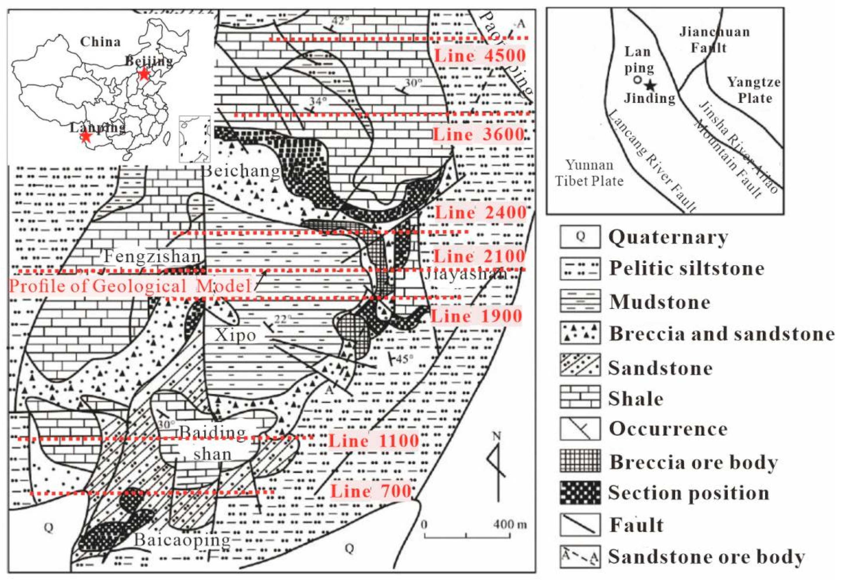
The Jinding lead–zinc deposit, located in Lanping County, Nujiang Prefecture, Yunnan Province, is the largest lead–zinc deposit in China (Figure 1). Due to the complicated geological and topographical conditions of the “Three-River” metallogenic belt, there are many disputes regarding the geological genesis and metallogenic model of the Jinding lead–zinc deposit [1,2]. Regarding its geological genesis, Wang, 2001; Yan, 1997; Zhu, 2016; Zhang, 2010; and Zeng, 2016, among others, have conducted extensive research but with different perspectives of the origin, including hydrothermal filling metasomatic type, stratabound epigenetic deposit, syngenetic sedimentary deposit, and exhalative (hydrothermal) sedimentary deposit [3,4,5,6,7,8]. Among them, the viewpoint of the exhalative (hydrothermal) sedimentary deposit dominates. However, some studies have shown that the Jinding lead–zinc deposit is more likely to be an epigenetic filling-type stratabound deposit, with this view supported by geological evidence such as the paleoenvironment of the ore-bearing strata. However, these geological research achievements lack support from geophysical exploration evidence, especially in the absence of establishing a geophysical model of the ore deposit related to geological genesis and mineralization patterns.

Geophysical modeling is known to be a crucial link in both theoretical research and production practices in geophysics. With the continuous development of geophysical exploration methods and technologies, the construction and research of geophysical models have become the key to the success of geophysical exploration. By constructing and studying geophysical models and using forward numerical simulations to validate exploration methods, the multiplicity of solutions in geophysical exploration inversion and interpretation can be reduced. Therefore, constructing a geophysical model for the Jinding lead–zinc deposit is particularly important for studying the geological genesis and mineralization patterns of the deposit.

In the Jinding mining area, geological surveys at scales of 1:200,000, 1:250,000, and 1:500,000; physical property measurements of rocks; and drilling verification work have been conducted. These geological data and lithological research findings provide a solid foundation for establishing a geophysical model. However, in terms of geophysical exploration, only AMT (audio-frequency magnetotellurics) surveys and 1:500,000 gravity exploration studies (Ma, 2019) have been carried out in different sections of the Jinding lead–zinc deposit; thus, systematic geophysical research is lacking [9]. In particular, the current success rate in exploring middle-to-deep concealed ores remains low, and mining enterprises are already facing a resource crisis. Therefore, further research on geophysical exploration methods and techniques for the Jinding deposit is essential to establish effective geophysical exploration models and prospecting strategies for future mineral resource exploration.

The controlled-source audio-frequency magnetotellurics (CSAMT) method, renowned for its robust anti-interference capabilities, extensive detection depth, and remarkable work efficiency, has emerged as a pivotal tool in deep resource exploration. Its applications (such as in Cao, 2010; Yu,1998; Wang, 2016; He, 2016) have yielded outstanding outcomes in mineral resource exploration, concealed ore body identification, and metallogenic prediction within complex geological terrains [10,11,12,13,14]. Therefore, based on the exploration objectives and requirements for the concealed ore bodies in the middle and deep parts of the mining area, the CSAMT method can be selected as the geophysical exploration approach for the Jinding lead–zinc deposit. By combining this with a geophysical model of the deposit, forward numerical simulations can be utilized to verify the effectiveness of the exploration method. At the same time, based on the forward simulation parameters, a geophysical technical solution suitable for exploring ore bodies in the Jinding deposit can be selected and optimized.

For general geoelectric models, CSAMT methods do not have simple numerical solutions and often require reliable numerical solutions to be sought. Traditional methods for solving CSAMT numerical solutions can be summarized into four main algorithms: the volume integral method, the boundary integral method, the finite difference method, and the finite element method. The finite element method has been adopted by many scholars (Jiang 2018; Tang 2014, Ren 2012, 2014, Yonghyun 2014, Yin 2014, Octavio 2015, Hunag 2016) due to its characteristics such as grid diversity and high calculation accuracy [15,16,17,18,19,20,21,22]. However, these studies share a common characteristic: the finite element calculations predominantly adopt traditional truncated boundaries, which approximate infinite boundary problems within a relatively large region as finite ones. This approach often leads to issues such as large calculation areas, high node counts, significant storage requirements, and time-consuming computations. A more reasonable boundary-handling strategy should limit the calculation area to a smaller target region, reducing the number of elements and nodes and thereby conserving computational resources and improving computational speed. The finite element–infinite element coupling method offers the possibility to implement this strategy. The core idea of finite element–infinite element coupling is to replace traditional truncated boundaries with “infinite elements.” By using coordinate mapping, “infinite elements” are infinitely extended in a certain direction, enabling the electromagnetic field to rapidly decay to zero within these elements. Finally, by combining finite elements to discretize the internal small region, rapid forward simulations can be achieved [23,24]. In the field of geophysics, the infinite element method is primarily applied in seismic exploration, well logging, and direct current (DC) resistivity methods. Gong (2019) successfully implemented this technique in numerical simulations of DC resistivity [25], but its application remains relatively limited in electromagnetic methods. Only Tang (2014) has conducted simple research on the application of infinite elements in CSAMT [16]. Therefore, conducting research on the geophysical model of the Jinding lead–zinc mining area with the coupled finite element–infinite element method has important guiding significance for the selection of geophysical exploration methods.

In traditional CSAMT field surveys, due to the complexity of electromagnetic theory and a lack of technical training, most operators can only follow the equipment manufacturer’s manual for fieldwork and data processing. Hence, a major challenge is the lack of effective quality control and evaluation of CSAMT data. For example, operators often focus on transmitter signal strength alone and neglect the quantitative evaluation of receiver signal strength. On the other hand, to improve efficiency, single-cycle data acquisition is commonly used, so the importance of time stacking for enhancing low-frequency data quality is often overlooked, leading to unclear or incorrect near-field characteristics in resistivity sounding curves. These practices significantly reduce the effectiveness of CSAMT exploration.

Therefore, in this study, the exploration of the Jinding lead–zinc mine was taken as an example. Firstly, based on existing geological survey results, geological models, and resistivity measurements of rocks in the mining area, research was conducted to construct a 3D geophysical model of the Jinding lead–zinc mine. Then, 3D forward modeling based on the finite element–infinite element method was used to numerically simulate the constructed geophysical model in order to verify the effectiveness of the CSAMT exploration method in the Jinding lead–zinc mine. Meanwhile, an optimal technical scheme for the CSAMT exploration of the mine was rationally designed based on the forward numerical simulation scheme.

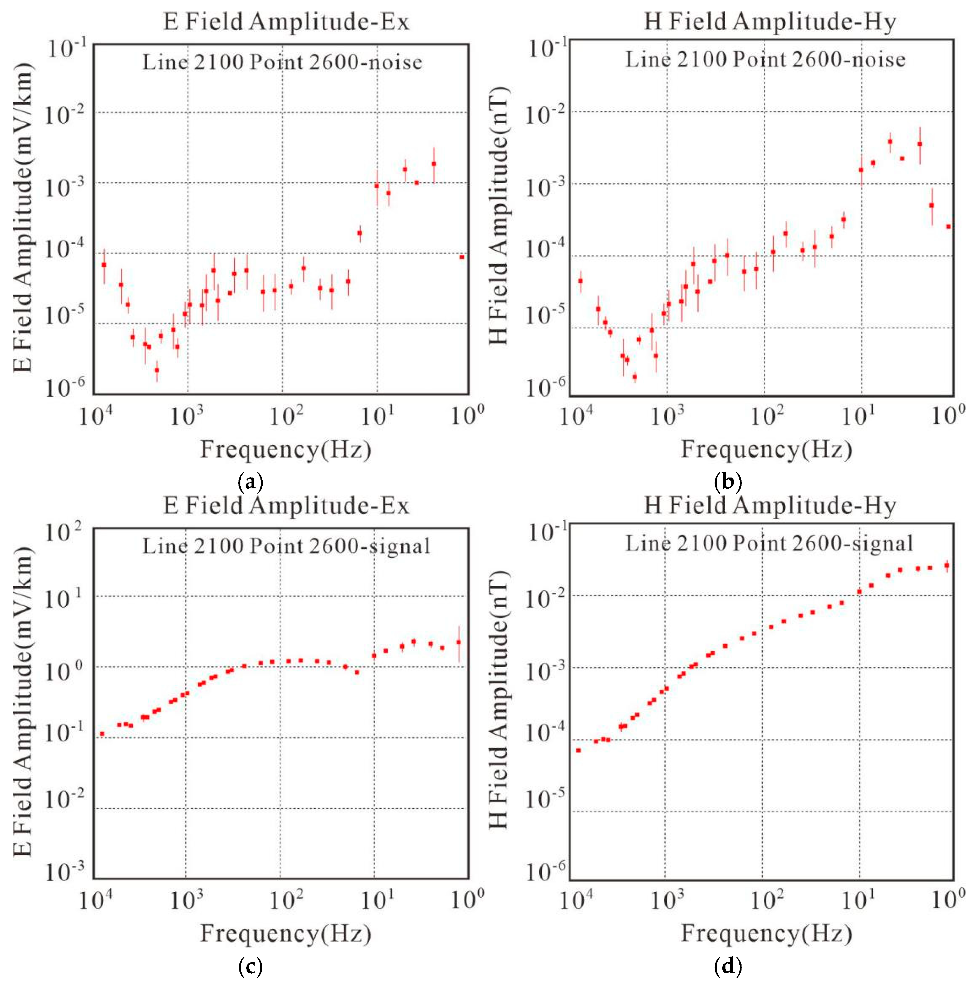
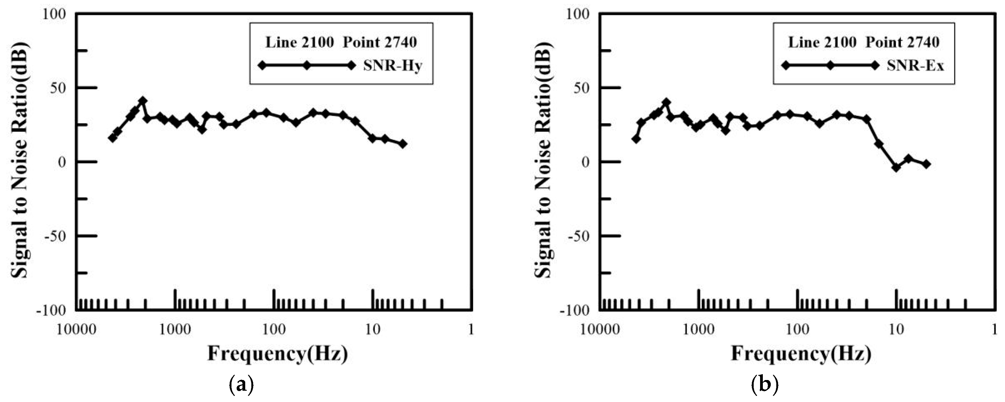
Secondly, field exploration using CSAMT was carried out in the Jinding mine to validate the field application’s effectiveness. Through noise testing experiments and acquisition time trials, optimal transmission intensity and acquisition time parameters were determined, significantly improving the quality of CSAMT field data acquisition. A new method for calculating the signal-to-noise ratio (SNR) using the electromagnetic background signals in the mining area as the noise source was proposed to quantitatively evaluate the quality of data acquisition. Additionally, methods for qualitatively evaluating data quality based on the transition zone and near-zone characteristics of the CSAMT Cagniard resistivity sounding curves were proposed.

Finally, the data obtained from the field exploration were inverted using a continuous medium inversion method to derive the 2D electrical structure characteristics of the deep part of the Jinding deposit, which were then interpreted. This provides rigorous geophysical evidence for the in-depth exploration of the deep metallogenic geological background and environment of the Jinding lead–zinc deposit.

The entire set of CSAMT geophysical exploration technical schemes mentioned above can provide geophysical exploration models, directions, and ore-finding ideas for mineral resource exploration in the Jinding and similar deposits.

2. Geological Overview and Geophysical Model

2.1. Geological Overview of the Deposit

The Jinding lead–zinc deposit is prominently situated within the densely compressed middle segment of the Sanjiang fold system, which is positioned precisely at the northern terminus of the Lanping–Simao Meso-Cenozoic depression. It is strategically positioned between the north–south-oriented faults tightly hemmed in by the Mishahe Fault Zone and the Lancang River Fault Zone and is found to the western flank of the Bihe River Fault Zone, within the ancient Lanping–Yunlong Paleocene graben basin. The deposit is divided into seven distinct mining sections, including Beichang, Jiayashan, Fengzishan, Paomaping, Xipo, Nanchang, and Baicaoping. The mining area exposes a succession of strata ranging from older to younger deposits, comprising the Upper Triassic Sanhedong Formation (T3s) of marine limestones (including brecciated limestones, dolomitic limestones, argillaceous limestones, and limestone mudstones), the Maichuqing Formation (T3m, the core strata of the syncline, with alternating layers of quartz sandstones and carbonaceous mudstones), the Middle Jurassic Huakaizuo Formation (J2h, interbedded layers of argillaceous siltstones, siltstones, and mudstones), the Upper Jurassic Bazhulu Formation (J2b, consisting of mudstones, argillaceous siltstones, and calcareous conglomerates), the Lower Cretaceous Jingxin Formation (K1j, with alternating layers of quartz sandstones, silty mudstones, and intercalated limestone conglomerates), the Upper Cretaceous Nanxin Formation (K2n, composed of argillaceous conglomerates, fine sandstones, siltstones, and mudstones), the Upper Cretaceous Hutousi Formation (K2h, characterized by long quartz sandstones), the Lower Tertiary Paleocene Yunlong Formation (E1y, interbedded layers of muddy gravelly rocks and argillaceous siltstones), the Guolang Formation (E2g, with alternating layers of argillaceous siltstones, silty mudstones, and intercalated fine sandstones), the Eocene Baoxiangsi Formation (Eb, featuring long quartz sandstones, conglomerates, sandstones, mudstones, and quartzites), the Upper Tertiary Pliocene Sanying Formation (N2s, with interbedded layers of conglomerates, sandy conglomerates, sandstones, and mudstones), and the Quaternary Pleistocene (Qp, with sand and gravel layers) and Holocene (Qh, comprising gravels, sand grains, and sandy clays).

The primary geological structure of the mining area is a thrust nappe tectonic assemblage, which constitutes a significant component of the large-scale thrust nappe structure that formed during the Paleocene Yunlong period in the Lanping Basin. Klippe structures, or flysch formations, exist in numerous segments throughout the mining area. Furthermore, thrust-sliding planes have also been incorporated into the tectonic domes, resulting in the formation of dome structures that are characterized by the co-deformation of both thrust tectonics and in situ systems. In accordance with these findings, it can be concluded that the thrust tectonics predate the formation of the dome structures, with their inception likely commencing as early as the late Yunlong period. In summary, the geological structures of the Jinding mining area are complex, characterized by well-developed folds and faults that exhibit multiple stages of activity. This underscores the dynamic and protracted geological history of the region. The geological structures of the mining area are primarily characterized by the Gaoping–Laomujing syncline, the Bihe River Fault, horizontal thrust faults, transverse faults, oblique faults, and secondary fault structures.

2.2. Geological and Geophysical Model of the Ore Deposit

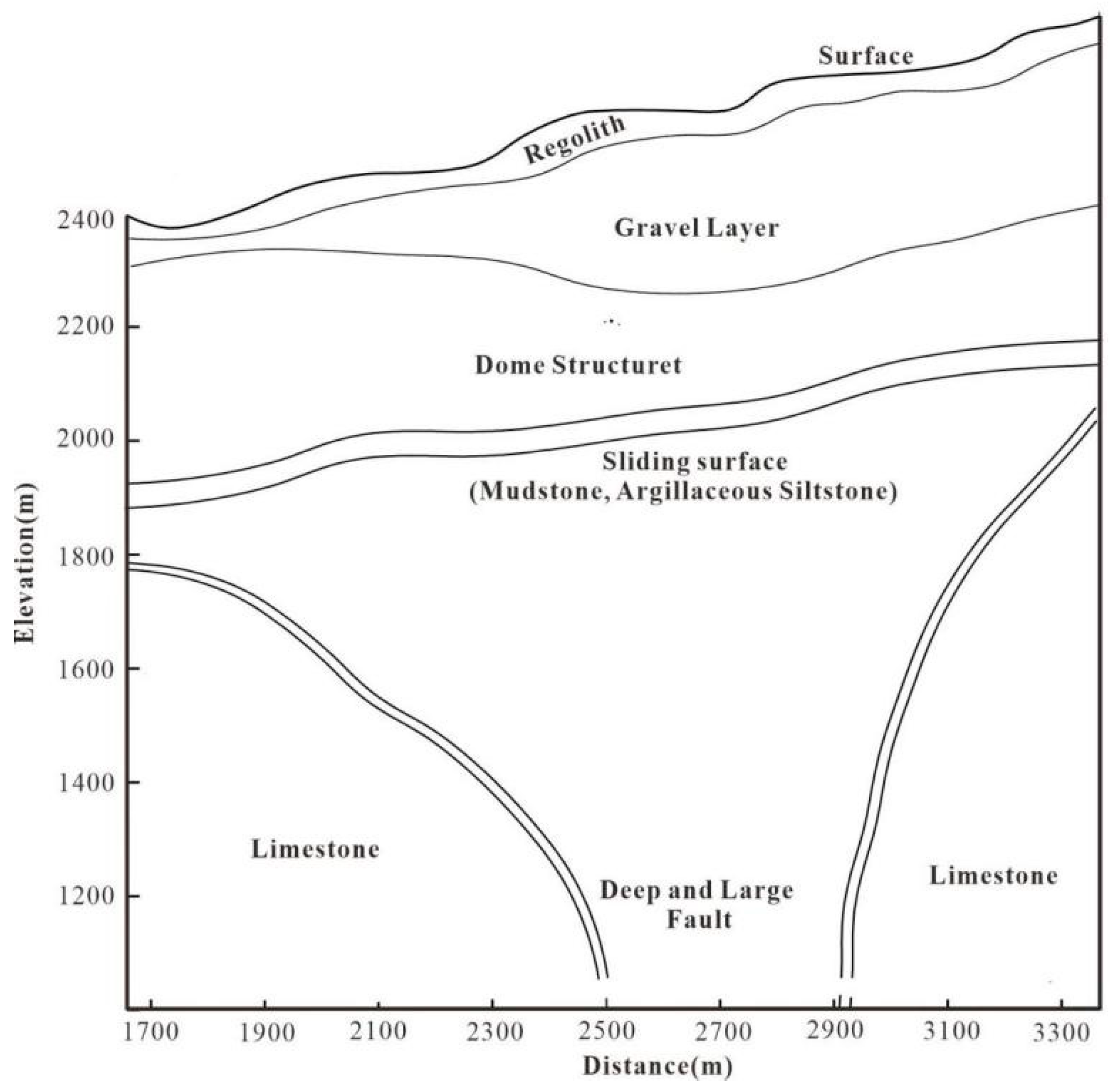
Based on existing geological data and previous research, our research group conducted an in-depth study on the geological model of the Jinding lead–zinc deposit and proposed a two-dimensional geological model of the deposit[], as shown in Figure 2.

In Figure 2, the shallow surface is a thin layer of soil and sand–gravel rock. Below it is a dome structure and a sliding surface mainly composed of mudstone and argillaceous silt. Between the sand–gravel rock and the dome structure, there are tabular, layered, and stratoid sandstone-type ore bodies. Below the fault structure are limestone and breccia ore bodies, and below these bodies is limestone. There are deep fractures between the limestone layers. To establish a geophysical model of the deposit, it is necessary to measure the electrical parameters of the geological model. For the resistivity parameters of rock ore, the SQ-3C dual-channel lightweight-induced polarization instrument is used to measure the resistivity and polarization amplitude/frequency of the rock samples using the forced current method.

Table 1. Electrical parameters of rocks (ores) in the Jinding lead–zinc deposit.

Rock/Ore Name	Average Polarizability ηs (%)	Average Resistivity (Ω·m)
Primary sandstone-type sulfide ore	20.57	521
Limestone breccia sulfide ore	4.83	3078
Lead–zinc oxidized quartz sandstone	3.16	1527
Oxidized ore	1.65	1578
Limestone	1.24	15,911
Sandstone	0.75	6584
Feldspar quartz sandstone	0.71	447
Quartz sandstone	0.76	412
Siltstone, fine sandstone	0.69	235
Argillaceous siltstone	0.63	202
Mudstone	0.67	186

shows the electrical properties of the rocks in the Jinding mining area. The resistivity of various rocks in the mining area can be divided into five levels. Limestone has the highest resistivity, above 10,000 Ω·m. Pure sandstone comes next, with a resistivity of around 6000 Ω·m. Limestone breccia-type sulfide ore has a resistivity of approximately 3000 Ω·m. Lead–zinc oxide ore has a resistivity of about 1500 Ω·m, and sandstone-type sulfide ore has a resistivity of 400–500 Ω·m. The lowest resistivity is found in mudstone, argillaceous siltstone, and fine sandstone, at approximately 200 Ω·m. The polarizability of mudstone, argillaceous siltstone, sandstone, and limestone is around 1.0%. Lead–zinc oxide ore has a polarizability of about 3.0%, and limestone breccia-type sulfide lead–zinc ore has a polarizability of about 4.5%. Primary sandstone-type sulfide ore has the highest polarizability, at around 20.0%.

The above analysis shows that mudstone, argillaceous siltstone, and fine sandstone have basically the same electrical characteristics, with a resistivity of between 100 and 200 Ω·m and a polarizability of less than 1%, indicating low resistivity and low polarizability. However, regardless of whether it is primary sulfide ore or oxidized ore, the resistivity of the ore body is between 400 and 500 Ω·m, and the polarizability is approximately 4–20%. As can be seen from the typical exploration profile in Figure 1, mudstone and argillaceous siltstone basically constitute the surrounding rocks of the lead–zinc ore body. Therefore, the lead–zinc ore body in the area should exhibit relatively high resistivity and high polarizability characteristics. When the surrounding rock is locally limestone, it exhibits low resistivity and high polarizability characteristics.

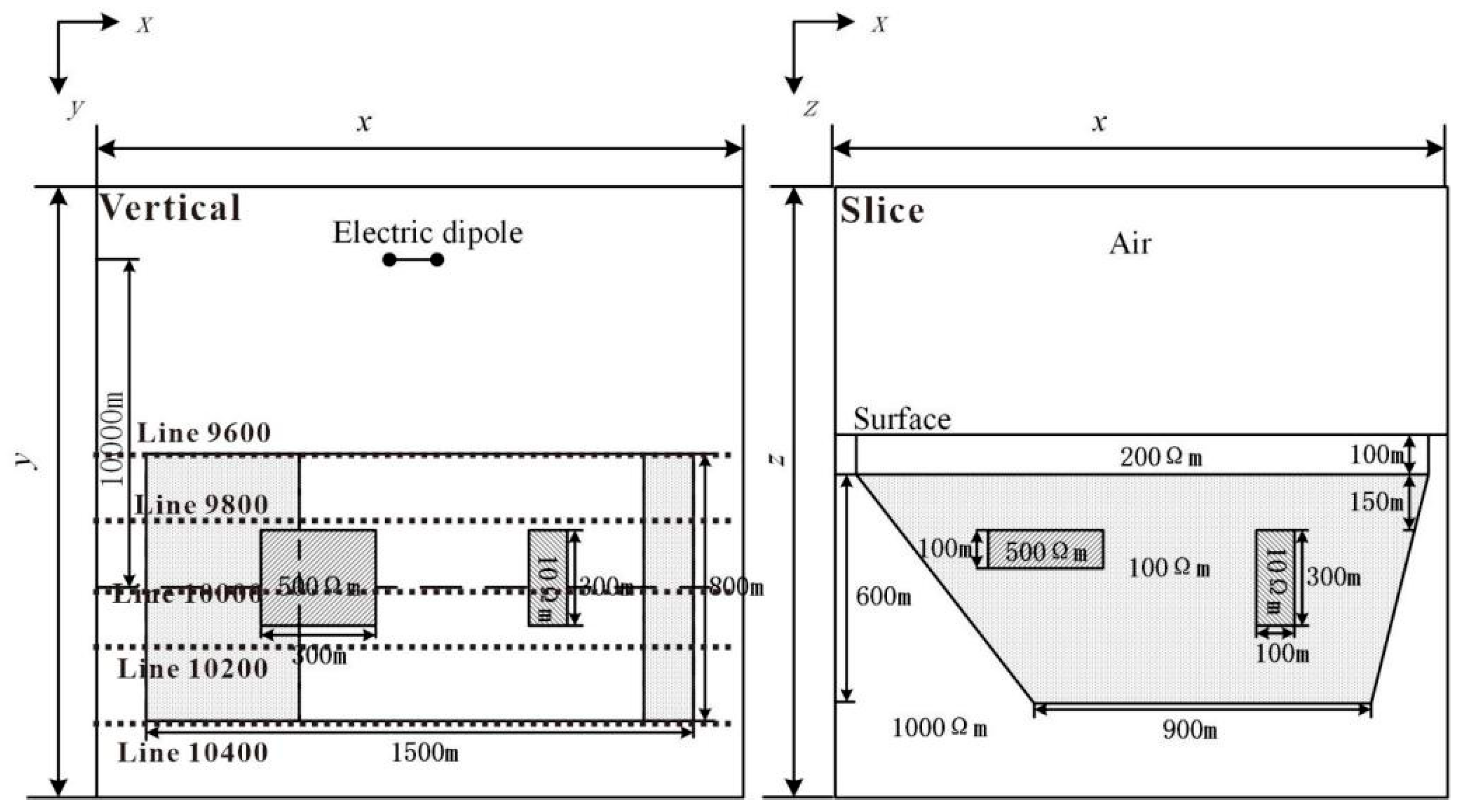
Therefore, based on the 2D geological model that uses the electrical parameters of rocks in the Jinding lead–zinc deposit (Table 1), a 3D geophysical model is constructed, as shown in Figure 3. In the figure, the first layer represents the surface covering layer with a thickness of 100 m. Its main component is sand and gravel strata, and it has an average resistivity of 200 $\Omega \mathrm{m}$. Beneath the covering layer lie domes and concealed deep fault structures with a resistivity of 100 $\Omega \mathrm{m}$. On both sides of the fault are high-resistance surrounding rocks with a resistivity of 1000 $\Omega \mathrm{m}$. The ore bodies are hosted within the dome structure, primarily consisting of sandstone-type and limestone breccia ore bodies. The sandstone ore body resembles a platy form, with a resistivity of 500 $\Omega \mathrm{m}$. Its dimensions are 300 m in length, 100 m in width, and 300 m in height. The limestone breccia ore bodies often appear as inclined or vertical thin layers, also with a resistivity of 500 $\Omega \mathrm{m}$, and their dimensions are 100 m in length, 300 m in width, and 300 m in height. The limestone breccia ore bodies often occur as inclined or vertical thin layers with a resistivity of 500 $\Omega \mathrm{m}$. Their dimensions are typically 100 m in length, 300 m in width, and 300 m in height.

3. Numerical Simulation of CSAMT

Numerical simulation research not only enhances people’s understanding and knowledge about the exploration methods but also assists in selecting the correct exploration approach and setting appropriate field acquisition parameters. Therefore, we employed a three-dimensional CSAMT forward modeling program based on the coupled finite element–infinite element method to conduct a numerical simulation on the geophysical model of the Jinding lead–zinc mine. Three-dimensional CSAMT forward modeling using the coupled finite element–infinite element method is an efficient numerical simulation technique for electromagnetic fields, which combines the advantages of the finite element method in handling complex geological structures and boundary conditions with the characteristics of the infinite element method in simulating infinite far-field attenuation. This method achieves rapid and high-precision forward modeling, reduces the computation domain and the number of nodes, accelerates the computation, and is of great significance to the development of exploration geophysics [20,21].

3.1. Fundamental Equation

The electric field generated by a horizontal electric dipole (time factor $e^{-i\omega t}$, angular frequency $\omega$) in an isotropic conductive medium satisfies the double curl equation [26]:

$$\nabla \times \nabla \times \overrightarrow{\mathbf{E}}-i\omega {\mu }_0\left(\sigma -i\omega {\epsilon }_0\right)\overrightarrow{\mathbf{E}}=i\omega {\mu }_0{J}_s,$$

(1)

where $\sigma$ is the resistivity, $J_s$ is the current density vector of the electric dipole, and the magnetic permeability ${\mu }_0$ of both the air and the subsurface medium is taken as the vacuum magnetic permeability, while the dielectric constant ${\epsilon }_0$ is the vacuum dielectric constant.

The electric dipole source exhibits singularity. The total electric field is decomposed into the sum of the background field ${\overrightarrow{\mathbf{E}}}^p$ (primary field) and the induced field ${\overrightarrow{\mathbf{E}}}^s$ (secondary field). The background field ${\overrightarrow{\mathbf{E}}}^p$ is directly solved using a one-dimensional geoelectric model [27], while the induced field ${\overrightarrow{\mathbf{E}}}^s$ is solved using the finite element method to avoid the calculation of source singularity.

$$\overrightarrow{\mathbf{E}}={\overrightarrow{\mathbf{E}}}^p+{\overrightarrow{\mathbf{E}}}^s$$

(2)

The background field ${\overrightarrow{\mathbf{E}}}^p$ also satisfies the double curl equation of the electric field. Equations (1) and (2) can be used to derive the double curl equation based on the secondary field ${\overrightarrow{\mathbf{E}}}^s$:

$$\nabla \times \nabla \times {\overrightarrow{\mathbf{E}}}^s+k^2{\overrightarrow{\mathbf{E}}}^s=i\omega {\mu }_0\left(\sigma -{\sigma }^p\right){\overrightarrow{\mathbf{E}}}^p,$$

(3)

where $k^2=-i\omega {\mu }_0\left(\sigma -i\omega {\epsilon }_0\right)$. We know that on an electrical interface, the normal component of the electric field is discontinuous, while nodal finite elements require the electromagnetic field to be continuous in the normal direction. Therefore, the obtained finite element solution is often inaccurate and needs to be corrected. In the source region, the electric field solution of nodal finite elements does not satisfy condition $\nabla \cdot \left(\epsilon \overrightarrow{\mathbf{E}}\right)=-\nabla \cdot \left(\overrightarrow{J}/i\omega \right)$; in the source-free region, it does not satisfy condition $\nabla \cdot \left(\epsilon \overrightarrow{\mathbf{E}}\right)=0$. A divergence correction condition needs to be added to Equation (3) [28].

$$\nabla \times \nabla \times {\overrightarrow{\mathbf{E}}}^s+k^2{\overrightarrow{\mathbf{E}}}^s+\nabla \cdot {\overrightarrow{\mathbf{E}}}^s=i\omega {\mu }_0\left(\sigma -{\sigma }^p\right){\overrightarrow{\mathbf{E}}}^p$$

(4)

3.2. Weak Solution Integral Form

Based on the weighted residual finite element method (Jin 2014) [28], the residual formula for Equation (4) is established:

$$r=\nabla \times \nabla \times {\overrightarrow{\mathbf{E}}}^s+k^2{\overrightarrow{\mathbf{E}}}^s+\nabla \cdot {\overrightarrow{\mathbf{E}}}^s-i\omega {\mu }_0\left(\sigma -{\sigma }^p\right){\overrightarrow{\mathbf{E}}}^p$$

(5)

Take any test function $\overrightarrow{\mathbf{V}}$ on the region $\Omega$:

$${\displaystyle {\iiint }_{\Omega }r}\cdot \overrightarrow{V}d\Omega =0$$

Then, we have

$${\displaystyle \underset{\Omega }{\int }\nabla \times \nabla \times \overrightarrow{{\mathbf{E}}^s}\cdot \overrightarrow{V}d\Omega +}{\displaystyle \underset{\Omega }{\int }{k}^2{\overrightarrow{\mathbf{E}}}^s\cdot \overrightarrow{V}d\Omega }+{\displaystyle \underset{\Omega }{\int }\nabla \cdot {\overrightarrow{\mathbf{E}}}^s\cdot \overrightarrow{V}d\Omega =}i\omega {\mu }_0{\displaystyle \underset{\Omega }{\int }\left(\sigma -{\sigma }^p\right){\overrightarrow{\mathbf{E}}}^p\cdot \overrightarrow{V}d\Omega }$$

(6)

Let S be the outer boundary surface of the region $\Omega$. Instead of using traditional truncated boundary conditions, infinite elements are employed. Within the infinite elements, the electromagnetic field decays to zero, so we have

$${\overrightarrow{\mathbf{E}}}^s=0 \mathrm{on} S$$

(7)

By applying Green’s theorem to the first vector, Equation (6) can be simplified to

$${\displaystyle \underset{\Omega }{\int }\left(\nabla \times \overrightarrow{V}\right)\cdot \left(\nabla \times {\overrightarrow{\mathbf{E}}}^s\right)d\Omega }+{\displaystyle \underset{\Omega }{\int }{k}^2{\overrightarrow{\mathbf{E}}}^s\cdot \overrightarrow{V}d\Omega +{\displaystyle \underset{\Omega }{\int }\nabla \cdot {\overrightarrow{\mathbf{E}}}^s\cdot \overrightarrow{V}d\Omega }=}i\omega {\mu }_0{\displaystyle \underset{\Omega }{\int }\left(\sigma -{\sigma }^p\right){\overrightarrow{\mathbf{E}}}^p\cdot \overrightarrow{V}d\Omega }$$

(8)

The finite element method is used to discretize the internal computation domain. Assuming there are n nodes in the internal computation domain, the j-th test function can be taken as

$${\displaystyle \underset{\Omega }{\int }\left(\nabla \times {\overrightarrow{V}}_j\right)\cdot \left(\nabla \times {\overrightarrow{\mathbf{E}}}^s\right)d\Omega }+{\displaystyle \underset{\Omega }{\int }{k}^2{\overrightarrow{\mathbf{E}}}^s\cdot {\overrightarrow{V}}_{j}d\Omega +{\displaystyle \underset{\Omega }{\int }\nabla \cdot {\overrightarrow{\mathbf{E}}}^s\cdot {\overrightarrow{V}}_{j}d\Omega }=}i\omega {\mu }_0{\displaystyle \underset{\Omega }{\int }\left(\sigma -{\sigma }^p\right){\overrightarrow{\mathbf{E}}}^p\cdot {\overrightarrow{V}}_{j}d\Omega }$$

(9)

3.3. Coupled Finite Element–Infinite Element Method

The coupled finite element–infinite element method divides the entire solution domain into a finite element region and an infinite element region, replacing the traditional outer boundary with the infinite element region. Finite element analysis and infinite element analysis are performed in the two regions, respectively, and they are combined through the assembly of the overall stiffness matrix to obtain the numerical solution.

Figure 4 is a schematic diagram of the division of finite element and infinite element calculation regions. In the figure, the finite element region is the target region, which includes the field source, target body, measurement points, etc.; the infinite element region extends from the boundary of the finite element region to infinity, serving as the boundary calculation region. Infinite element analysis involves using infinite element mapping and shape functions in a certain direction within this region to map the global coordinates to local coordinates. Its principle is the same as that of finite element analysis.

• Finite Element Analysis

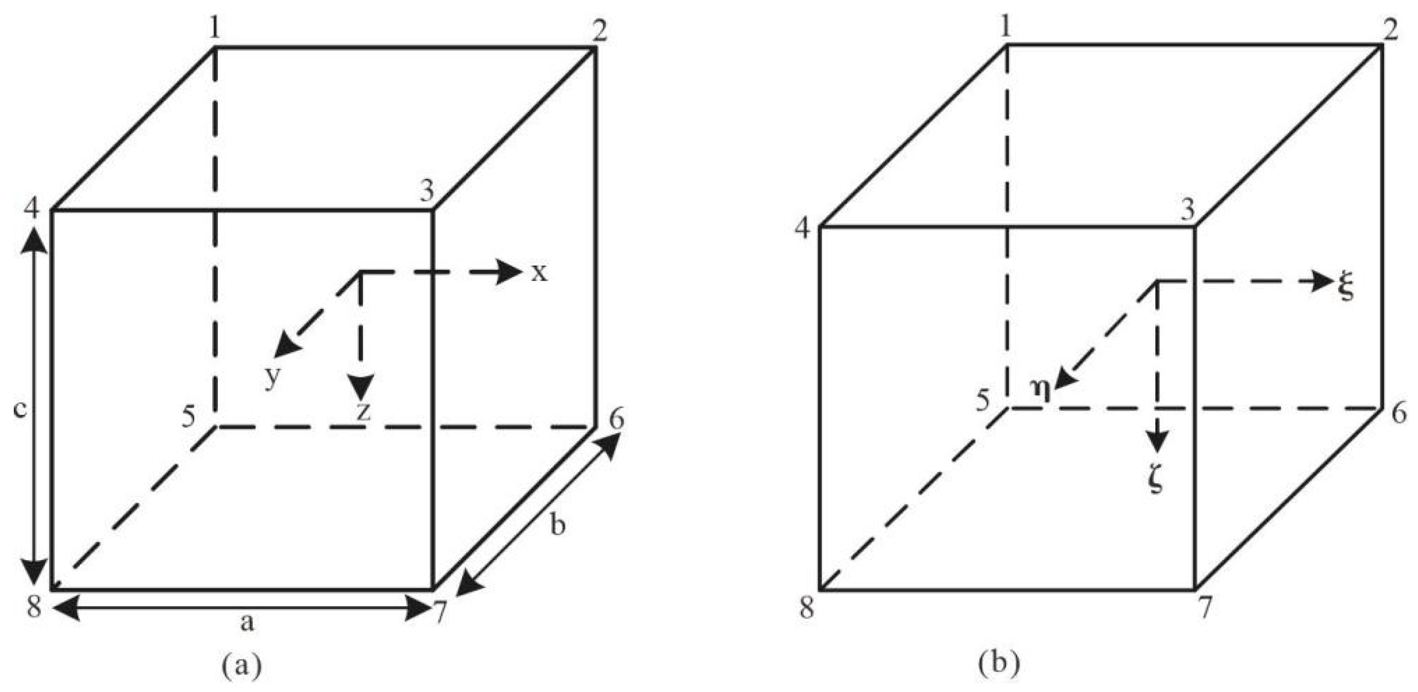
When performing finite element analysis, the rectangular hexahedron is used for regional discretization, and the element node numbering and coordinates are shown in Figure 5.

In Figure 5, the corresponding relationship between the coordinates of the parent and child elements is as follows:

$$x=x_0+{\displaystyle \frac{a}{2}}\xi \begin{array}{ccc}& & \end{array}y=y_0+{\displaystyle \frac{b}{2}}\eta \begin{array}{ccc}& & \end{array}z=z_0+{\displaystyle \frac{c}{2}}\zeta ,$$

(10)

where $x_0$, $y_0$, and $z_0$ represent the midpoint of the child element and a, b, and c represent the three side lengths of the child element. The expression for the shape function of the rectangular hexahedron is as follows:

$$N_i^e={\displaystyle \frac{1}{8}}(1+{\xi }_i\xi )(1+{\eta }_i\eta )(1+{\zeta }_i\zeta )$$

(11)

In the equation, ${\xi }_i$, ${\eta }_i$, and ${\zeta }_i$ represent the coordinates of node i in the child element within the parent element.

2.

Infinite Element Analysis

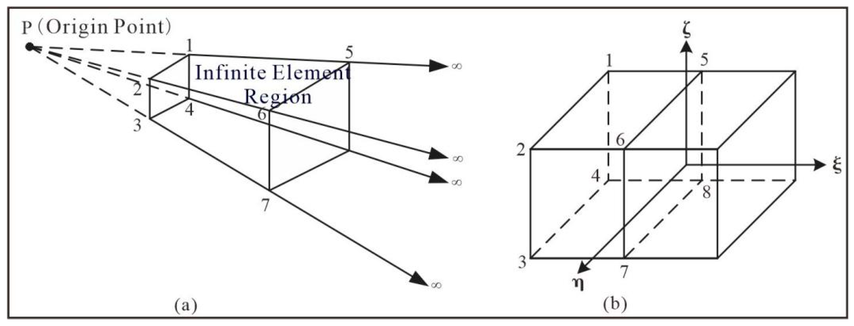
When performing infinite element analysis, a three-dimensional eight-node Astley-type infinite element is used [29]. Figure 6 presents a schematic diagram of three-dimensional infinite element mapping, where nodes 1, 2, 3, 4, 5, 6, 7, and 8 are the basic elements of the infinite element. P is the coordinate origin, and nodes 1, 2, 3, and 4 are the four nodes of a finite element on the boundary. The distances from point P to nodes 5, 6, 7, and 8 are twice the distances from point P to nodes 1, 2, 3, and 4, respectively. Infinite element analysis involves mapping infinite coordinates to the local coordinates in Figure 6b through infinite element mapping. In Figure 6b, the four outermost nodes of the infinite element represent infinity, and their field values are zero.

In Figure 6b, $\xi$ represents the mapping direction of the infinite element. Within plane $\zeta -\eta$, the infinite element and the finite element adopt the same mapping form and shape function. The coordinate mapping for the infinite element is as follows:

$$y={\displaystyle \sum _{i=1}^2{L}_i{y}_i}\begin{array}{ccc}& & \end{array}z={\displaystyle \sum _{i=1}^2{L}_i{z}_i},$$

(12)

$L_i$ represents the area of the quadrilateral, $L_i={\displaystyle \frac{1}{4}}\left(1+{\eta }_i\eta \right)\left(1+{\zeta }_i\zeta \right)$.

Combining the coordinate mapping relationship in direction $\zeta$, the coordinate mapping function for the eight-node infinite element can be obtained:

$$x={\displaystyle \sum _{i=1}^8{N}_i{x}_i}\begin{array}{cc}& \end{array}y={\displaystyle \sum _{i=1}^8{N}_i{y}_i}\begin{array}{cc}& \end{array}z={\displaystyle \sum _{i=1}^8{N}_i{z}_i},$$

(13)

where

$$\begin{array}{l}\left\{\begin{array}{c}{N}_i=L_i{\displaystyle \frac{1-\zeta }{2}}{\displaystyle \frac{-\left(1-\zeta \right)}{2}}\\ N_{i+4}=L_i{\displaystyle \frac{1-\zeta }{2}}\left(1-{\zeta }^2\right)\end{array}\right.\begin{array}{cc}& \end{array}i=1,2,3,4\\ SNR=20\ast Log{\displaystyle \frac{signal}{noise}}\end{array}$$

(14)

$N_i$ is the quadrilateral surface element mapping, and $L_i$ is the linear interpolation of area coordinates.

For the shape function of the infinite element, its specific expression is as follows:

$$\left\{\begin{array}{l}{M}_i=L_i{\displaystyle \frac{1-\xi }{2}}{\displaystyle \frac{-(1-\xi )}{2}}\xi \hfill \\ M_{i+4}=L_i{\displaystyle \frac{1-\xi }{2}}(1-{\xi }^2)\hfill \end{array}\begin{array}{cccc}& & & \end{array}\right.i=1,2,3,4,$$

(15)

This shape function is the product of coefficient A, which is used in the shape function adopted in the Astley mapped infinite element theory (Astley, 1994) and a second-order Lagrange interpolation polynomial [29].

The finite element and infinite element analyses are basically consistent, with both being eight-node elements. Therefore, in numerical simulations, the infinite elements and finite elements can be perfectly combined to ensure the symmetry of the stiffness matrix, making the solution simple and convenient.

3.4. Solving the Equation System

In the three-dimensional numerical simulation of CSAMT, each node has three degrees of freedom in the x, y, and z directions. Therefore, we take

$$\begin{array}{l}{\overrightarrow{V}}_j=\left({\overrightarrow{V}}_j^x,{\overrightarrow{V}}_j^y,{\overrightarrow{V}}_j^z\right)\begin{array}{cc}& \end{array}\begin{array}{c}{\overrightarrow{V}}_j^x=(N_j,0,0)\end{array}\begin{array}{cc}& \end{array}{\overrightarrow{V}}_j^y=(0,N_j,0)\begin{array}{cc}& \end{array}{\overrightarrow{V}}_j^z=(0,0,N_j)\\ {\overrightarrow{E}}^s=\left({\overrightarrow{E}}_x^s,{\overrightarrow{E}}_y^s,{\overrightarrow{E}}_z^s\right)\begin{array}{cc}& \end{array}{\overrightarrow{E}}_x^s={\displaystyle \sum _{i=1}^n{N}_i}{\overrightarrow{E}}_i^x\begin{array}{cc}& \end{array}{\overrightarrow{E}}_y^s={\displaystyle \sum _{i=n+1}^{2n}{N}_i}{\overrightarrow{E}}_i^y\begin{array}{cc}& \end{array}{\overrightarrow{E}}_z^s={\displaystyle \sum _{i=2n+1}^{3n}{N}_i}{\overrightarrow{E}}_i^z\end{array},$$

(16)

where $N_j$ is the shape function of the j-th measurement point, and its specific form is detailed in Equations (11) and (13).

Equation (9) can be written as follows:

$$\begin{array}{l}{\displaystyle \underset{\Omega }{\int }\left(\nabla \times {\overrightarrow{V}}_j^x\right)\cdot \left(\nabla \times {\overrightarrow{E}}^s\right)d\Omega }+{\displaystyle \underset{\Omega }{\int }{k}^2{\overrightarrow{E}}^s\cdot {\overrightarrow{V}}_j^{x}d\Omega +{\displaystyle \underset{\Omega }{\int }\nabla \cdot {\overrightarrow{E}}^s\cdot {\overrightarrow{V}}_j^{x}d\Omega }=}i\omega {\mu }_0{\displaystyle \underset{\Omega }{\int }\left(\sigma -{\sigma }^p\right){\overrightarrow{E}}^p\cdot {\overrightarrow{V}}_j^{x}d\Omega }\\ {\displaystyle \underset{\Omega }{\int }\left(\nabla \times {\overrightarrow{V}}_j^y\right)\cdot \left(\nabla \times {\overrightarrow{E}}^s\right)d\Omega }+{\displaystyle \underset{\Omega }{\int }{k}^2{\overrightarrow{E}}^s\cdot {\overrightarrow{V}}_j^{y}d\Omega +{\displaystyle \underset{\Omega }{\int }\nabla \cdot {\overrightarrow{E}}^s\cdot {\overrightarrow{V}}_j^{y}d\Omega }=}i\omega {\mu }_0{\displaystyle \underset{\Omega }{\int }\left(\sigma -{\sigma }^p\right){\overrightarrow{E}}^p\cdot {\overrightarrow{V}}_j^{y}d\Omega }\\ {\displaystyle \underset{\Omega }{\int }\left(\nabla \times {\overrightarrow{V}}_j^z\right)\cdot \left(\nabla \times {\overrightarrow{E}}^s\right)d\Omega }+{\displaystyle \underset{\Omega }{\int }{k}^2{\overrightarrow{E}}^s\cdot {\overrightarrow{V}}_j^{z}d\Omega +{\displaystyle \underset{\Omega }{\int }\nabla \cdot {\overrightarrow{E}}^s\cdot {\overrightarrow{V}}_j^{z}d\Omega }=}i\omega {\mu }_0{\displaystyle \underset{\Omega }{\int }\left(\sigma -{\sigma }^p\right){\overrightarrow{E}}^p\cdot {\overrightarrow{V}}_j^{z}d\Omega }\end{array},$$

(17)

Using the vector curl formula and the divergence formula, Equation (17) above can be simplified and written in matrix form as follows:

$$Ax=b,$$

(18)

where

$$\begin{gathered} A={\displaystyle \underset{\Omega }{\int }\left[\begin{array}{l}{\displaystyle \sum _{i=1}^n\left(\frac{\partial N_i}{\partial z}\frac{\partial N_j}{\partial z}+\frac{\partial N_i}{\partial y}\frac{\partial N_j}{\partial y}+\frac{\partial N_i}{\partial x}\frac{\partial N_j}{\partial x}+k^2{N}_i{N}_j\right)}\begin{array}{ll}& -{\displaystyle \sum _{i=1}^n\frac{\partial N_i}{\partial x}\frac{\partial N_j}{\partial y}\begin{array}{ll}& -{\displaystyle \sum _{i=1}^n\frac{\partial N_i}{\partial x}\frac{\partial N_j}{\partial z}}\end{array}}\end{array}\\ -{\displaystyle \sum _{i=1}^n\frac{\partial N_i}{\partial y}\frac{\partial N_j}{\partial x}\begin{array}{ll}& {\displaystyle \sum _{i=1}^n\left(\frac{\partial N_i}{\partial z}\frac{\partial N_j}{\partial z}+\frac{\partial N_i}{\partial y}\frac{\partial N_j}{\partial y}+\frac{\partial N_i}{\partial x}\frac{\partial N_j}{\partial x}+k^2{N}_i{N}_j\right)\begin{array}{ll}& -{\displaystyle \sum _{i=1}^n\frac{\partial N_i}{\partial y}\frac{\partial N_j}{\partial z}}\end{array}}\end{array}}\\ -{\displaystyle \sum _{i=1}^n\frac{\partial N_i}{\partial z}\frac{\partial N_j}{\partial x}\begin{array}{ll}& -{\displaystyle \sum _{i=1}^n\frac{\partial N_i}{\partial z}\frac{\partial N_j}{\partial y}\begin{array}{ll}& {\displaystyle \sum _{i=1}^n\left(\frac{\partial N_i}{\partial z}\frac{\partial N_j}{\partial z}+\frac{\partial N_i}{\partial y}\frac{\partial N_j}{\partial y}+\frac{\partial N_i}{\partial x}\frac{\partial N_j}{\partial x}+k^2{N}_i{N}_j\right)}\end{array}}\end{array}}\end{array}\right]}dV \\ b=i\omega {\mu }_0{\displaystyle \underset{\Omega }{\int }\left(\sigma -{\sigma }^p\right){\left(\begin{array}{ccc}{N}_j{\overrightarrow{E}}_x^p& N_j{\overrightarrow{E}}_y^p& N_j{\overrightarrow{E}}_z^p\end{array}\right)}^{T}d\Omega } \end{gathered}$$

(19)

Equation (18) is a large, sparse, and symmetric complex coefficient linear equation system. In this system, matrix A represents the overall stiffness matrix of the coupled finite element–infinite element method, which is a $3\times N_x\times N_y\times N_z$ square matrix. Here, $N_x$, $N_y$, and $N_z$ denote the total number of nodes in the x, y, and z directions, respectively. Each row in matrix A has a maximum of 81 non-zero elements. x represents the electric field values at each node that need to be solved; b is the right-hand side term, which includes the anomalous body and the primary field. For solving large-scale sparse linear equation systems, this study adopts Pardiso, an open-source solver with excellent performance and high parallelization. Pardiso uses LU decomposition for direct solving, making it particularly suitable for handling multi-source CSAMT problems.

3.5. Forward Modeling of the Jinding Lead–Zinc Geophysical Model

The coupled finite element–infinite element method was used for the following numerical simulation and forward modeling calculation parameters:

In the x direction, the subdivision area ranges from −3000 to 15,000. Within the survey line area, the grid size is set to 50 m, resulting in a total of 121 nodes.

In the y direction, the subdivision area ranges from −3000 to 3000. Within the survey line area, the grid size is set to 50 m, resulting in a total of 63 nodes. Near the field source and the target body, the grid subdivision is relatively dense.

In the z direction, the subdivision area ranges from −3200 to 3000, with a total of 36 nodes. The air region spans from −3200 to 0 and is subdivided into six layers. Due to the rapid attenuation of the field in underground media, the grid subdivision size is smaller, and the grid size is set to 25 m.

Frequencies: 8192, 4096, 2048, 1024, 512, 256, 128, 64, 32, 16, 8, 4, 2, and 1 Hz, totaling 14 frequencies. The average calculation time for each frequency point is approximately 240 s.

To demonstrate the advancement of the coupled finite element–infinite element method proposed in this paper.

Table 2. Comparison of computational efficiency between the finite element method and the coupled finite element–infinite element method (computation frequency: 256 Hz).

Method	Meshes	Freedoms	Discrete Region (Km × Km × Km)	Memory (GB)	Computing Time (s)
Finite element	463,680	1,391,040	57.2 × 56.8 × 40	51.3 GB	461
Finite element–infinite element	274,428	823,284	6 × 18 × 6.2	24.8 GB	255

shows the computational data of the traditional large-scale finite element method and the finite element–infinite element coupling method(computation frequency: 256 Hz). In Table 2, the coupled finite element–infinite element method has a small discrete area, accounting for only 1% of the traditional finite element method. The total number of degrees of freedom is reduced by 40%. In terms of memory, the finite element–infinite element method reduces memory usage by 57%. In terms of computation time, the finite element–infinite element method improves the calculation speed by 45%. Therefore, the coupled finite element–infinite element method has obvious advantages such as a small discrete area, fewer computational nodes, and a faster solution speed compared to the traditional large-scale finite element method.

The numerical simulation results are presented in Figure 7. In Figure, from left to right, the vertical source–receiver distances of the five survey lines are 9600 m, 9800 m, 10,000 m, 10,200 m, and 10,400 m, respectively (Figure 3). From the apparent resistivity pseudo-section map, it can be observed that the CSAMT 3D forward modeling results exhibit a significant response to the low-resistivity dome structure of the Jinding lead–zinc deposit, providing a clear reflection of the structure’s morphology. However, due to the boundary effects, the boundary between the dome structure and the high-resistivity limestone is relatively blurred. In addition, due to the low-resistivity shielding effect of electromagnetic methods, the relatively high-resistivity lead–zinc ore bodies show little response in the simulation. Based on the numerical simulation results, it can be seen that when exploring high-resistivity target bodies in low-resistivity surrounding rocks, the CSAMT electromagnetic response is weak, and the numerical effect is not significant. However, when exploring low-resistivity structures such as faults and fracture zones in high-resistivity surrounding rocks, the effect is very pronounced. Therefore, it is feasible to conduct CSAMT exploration research in the Jinding lead–zinc mining area to identify low-resistivity faults, dome structures, and other features within the ore deposit.

Additionally, the forward modeling parameters used in the 3D CSAMT numerical simulation, such as grid size, vertical source–receiver distance, frequency band range, survey line length, and the three-dimensional size and location of the target body, can assist us in designing the field CSAMT acquisition parameters to achieve good exploration results.

4. CSAMT Experiment in the Jinding Lead–Zinc Deposit

The objective of CSAMT exploration is to obtain data on the electrical structure within a depth of 1 km below the surface of the mining area, which can help us understand the deep geological background and mineralization environment. At the same time, it can provide geophysical evidence for geological researchers to study the genesis of the Jinding lead–zinc deposit, which can help predict and delineate the mineralization target areas.

4.1. CSAMT Acquisition Design

4.1.1. Line Layout

For CSAMT field data acquisition, a total of seven survey lines were laid out. The specific locations of the survey lines are shown in Figure 1. From bottom to top, they are Line 700, Line 1100, Line 1900, Line 2100, Line 2400, Line 3600, and Line 4500. The total length of the survey lines is 13.68 km. Among them, Lines 1900, 2100, and 2400 cross the main ore body and are the key research objects.

4.1.2. Acquisition Parameters

The parameters for CSAMT field data acquisition mainly consist of two parts: transmitter parameters and receiver parameters. The transmitter operating parameters primarily include the transmitter position (transmitter–receiver distance), dipole length: AB, ground resistance: RAB, transmitting current: I, and transmitting frequency: f. The receiver operating parameters mainly include the measurement mode, receiver MN length, and acquisition time.

For this CSAMT field measurement, the transmitter dipole is AB = 2.25 km, and the ground resistance is RAB = 20 $\Omega \mathrm{m}$. To ensure an exploration depth exceeding 1 km, based on the previous forward modeling parameters, the transmitter–receiver distance is set to between 10.8 km and 14.2 km. The transmitting frequency ranges from 7680 Hz to 0.9375 Hz, with a total of 52 frequency points. The dipole spacing is MN = 40 m. The CSAET method is adopted for the field CSAMT measurement, with six channels of electric field data and one channel of magnetic field data collected each time. Two sets of V8 multifunctional electrical instruments are used for field data acquisition.

4.2. CSAMT Data Quality Control

For field data acquisition, the strength of the received signal and the duration of data collection are crucial to the quality of CSAMT data acquisition. Therefore, in this CSAMT field measurement, on the one hand, the signal-to-noise ratio was calculated through white noise measurement experiments to judge the strength of the received signal, and the transmission signal strength was adjusted accordingly. On the other hand, through data collection time experiments, the quality of measurement data under different collection times was analyzed to determine the optimal data collection time scheme.

4.2.1. CSAMT Signal-to-Noise Ratio Experiment

To calculate the signal-to-noise ratio (SNR) of CSAMT data, both the noise signal and the data signal need to be obtained. Firstly, the open-pit mine at the center of the work area was selected as the experimental site. Data acquisition was conducted when the artificial field source was not transmitting, and the measured signals were considered noise signals. Secondly, under the same experimental setup conditions, when the artificial field source was transmitting, the collected signals were considered data signals. Finally, the signal-to-noise ratio (SNR) formula was used to calculate the SNR. By comparing the SNR values, the quality of the collected data was evaluated, which further indicated the strength of the received signal. The experimental results of the signal-to-noise ratio are shown in Figure 8.

In Figure 8, there are four sub-figures: the electric field noise signal amplitude diagram, the magnetic field noise signal amplitude diagram, the electric field data signal amplitude diagram, and the magnetic field data signal amplitude diagram. From the experimental results, it can be observed that the noise signals have a large range of amplitude value fluctuations and significant error bars. Conversely, the data signals exhibit smooth and continuous amplitude curves with small error bars, and their values are more than 10 times those of the noise signals. Therefore, the signal-to-noise ratio experiment we designed is reasonable and feasible and can be used as a criterion for evaluating the strength of the received signal.

The calculation formula for the signal-to-noise ratio is as follows:

$$SNR=20\ast Log{\displaystyle \frac{signal}{noise}}$$

(20)

The calculation results of the signal-to-noise ratio for the electric field and the magnetic field at the test point are shown in Figure 9.

In Figure 9, within the frequency band of 5000–10 Hz, the signal-to-noise ratio of both the electric field and the magnetic field is greater than 20 dB, and the noise percentage is less than 10%. This indicates that the signal strength is sufficiently large, and the quality of the measured CSAMT field data is high. In the high-frequency and low-frequency bands, the SNR is less than 10 dB, and the noise percentage is greater than 30%, indicating the low quality of the collected data. This is due to two main reasons: the V8 instrument and magnetic probe exhibit response distortion in both high- and low-frequency bands, resulting in low measurement accuracy; and when transmitting high frequencies, the transmission current is small, making the signal more susceptible to interference; in the case of low frequencies, factors such as shorter data collection time and stronger interfering signals contribute to a relatively lower signal-to-noise ratio in the data.

4.2.2. CSAMT Data Acquisition Time Experiment

During the field work, we also conducted experiments on acquisition time and obtained apparent resistivity sounding curves for different acquisition times. Through comparative analysis, we determined the optimal acquisition time parameters.

Experimental conditions: With a single acquisition cycle of 40 min, three acquisition times of 40, 80, and 120 min were selected. Under the same survey line, survey point, equipment, and field source, three apparent resistivity sounding curves were obtained. The experimental results for the different acquisition times are shown in Figure 9.

As can be observed in Figure 10, the apparent resistivity sounding curve with an acquisition time of 40 min exhibits poor continuity of resistivity values, especially below 30 Hz. The apparent resistivity curve appears jagged, and the characteristics of the transition zone and the near zone are not pronounced, indicating poor data quality. Compared to the apparent resistivity curve for the 40 min acquisition time, the apparent resistivity sounding curve for 80 min is smoother and more continuous, with smaller jumps. Below 30 Hz, it starts to enter the near zone, and the curve rises at an angle exceeding 45°. Meanwhile, there are jump points, and the transition zone characteristics are not pronounced, indicating intermediate data quality. The apparent resistivity sounding curve for the 120 min acquisition time is smooth and exhibits good continuity. The characteristics of the far zone, the transition zone, and the near zone are distinct. A minimum value appears at 10 Hz, which is a characteristic of the transition zone. Below 10 Hz, the sounding curve rises at an almost 45-degree angle, which is a typical characteristic of a CSAMT sounding curve, indicating high data quality.

Therefore, in the Jinding lead–zinc mining area, by extending the data acquisition time and increasing the stacking number, the characteristics of the apparent resistivity sounding curve at the measurement points can be significantly improved, thereby enhancing the quality of CSAMT single-point data.

4.3. CSAMT Data Processing

Before inversion, CSAMT data processing mainly includes the elimination of flying points and the smoothing of the Cagniard apparent resistivity and phase data at each measurement point, as well as the static correction and spatial filtering of apparent resistivity and phases along the entire survey line. Figure 11 shows the apparent resistivity frequency sounding curve obtained after data processing for some of the measurement points. From Figure 11, it can be seen that the apparent resistivity curve is smooth, continuous, and has a clear morphology. The characteristics of the far zone, transition zone, and near zone of the curve are obvious, which conform to the standards of CSAMT apparent resistivity sounding curves.

Figure 12a shows the original pseudo-section of the frequency of apparent resistivity for Line 2100. It can be seen from the figure that due to the influence of uneven geological bodies and topographic fluctuations on the surface, the Cagniard apparent resistivity varies greatly and exhibits “noodle-like” characteristics in the vertical direction, indicating severe static effects that require processing. Figure 12b is a diagram of the frequency of the apparent resistivity pseudo-section after static correction and spatial filtering. It can be seen from the figure that after processing, the apparent resistivity data change smoothly; the vertical “noodle-like” phenomenon disappears, and the static effects are well suppressed.

From the sounding curves of apparent resistivity at the measurement points and the pseudo-section diagram of the frequency of apparent resistivity along the survey line, it can be seen that compared with the original data, the processed data have achieved significant suppression in terms of static effects. The data are authentic, reliable, and of high quality, making them suitable for further inversion.

4.4. CSAMT Inversion

Because the direction of the survey lines is perpendicular to the trend of the ore body, we can use two-dimensional continuous medium inversion software to invert CSAMT data. The principle of continuous medium inversion is based on the assumption of a continuous variation in electrical properties in the subsurface. It discretizes the subsurface space using numerical methods and adjusts the resistivity values of each unit to achieve the best fit between the forward electromagnetic field data and the observed data. The method is closer to the real subsurface conditions and is suitable for exploration in complex geological settings, providing higher-precision information on the subsurface electrical structure [30,31].

Based on the statistics of the work area, the frequency of measurement points entering the near zone is around 10 Hz, and the surface resistivity ranges between 100 and 200 ohm per meter. According to the skin depth formula calculation, the exploration depth is approximately 1.5 km, which meets the exploration requirements. Therefore, we selected a total of 40 frequency points in the 8192–10 Hz frequency band for inversion. The initial inversion model is the result of one-dimensional Bostick inversion. After 34 iterations of inversion, the data misfit is 2.7.

5. Electrical Structure Interpretation of the Jinding Lead–Zinc Mine

5.1. Physical Property Analysis

To interpret the electrical structure detected using CSAMT, we used the two-dimensional inversion results of Line 1100 as a reference section. The main reason for selecting Line 1100 is that it has abundant borehole data, covering most of the stratigraphic lithologic units (including ore bodies) and major structural interfaces (including thrust nappes) in the mining area. The interpretation method we adopted involves combining the shallow subsurface electrical structure with borehole data and then conducting a comparative analysis with the inversion results.

As shown in Figure 13, the profile exhibits a low-resistivity background. The central low-resistivity body primarily consists of fine sandstone, siltstone, and limestone breccia containing lead–zinc ore and gypsum, with localized fault breccia zones. The center of the high-resistivity body is entirely composed of continuous fine sandstone and siltstone strata containing gypsum. Limestone and limestone breccia siltstone, as well as mudstone, sandstone, and siltstone containing gypsum, exhibit moderate or high resistivity. From the above electrical patterns, it can be observed that the resistivity of geological bodies is controlled by the material composition and transport properties of the rocks themselves, with a more pronounced influence from the transport properties. Therefore, the electrical structures of the subsequent survey line profiles are interpreted based on the electrical characteristics of the aforementioned geological bodies.

5.2. Interpretation of the Electrical Structure

The relative positions of the survey lines on the plane are shown in Figure 8. Line 4500 and Line 3600 are located on the north side of the PaoMaping mining area; Line 2400, Line 2100, and Line 1900 pass through the Jiayashan mining area; and Line 1100 and Line 700 are located on the west side of the Nanchang mining area. The north–south span of the survey lines is approximately 3.8 km, and all survey line profiles are oriented east–west, which provides assistance for comparing the three-dimensional spatial positions of the underground electrical structures. Due to the significant differences and distinct contrasts in resistivity presented in the two-dimensional continuous medium inversion results, as well as the abundant details in the electrical structures, the interpretation of the electrical structures primarily relies on the two-dimensional inversion results.

1.

Line 2400

Line 2400, Line 2100, and Line 1900 are located in the Jiayashan mining segment of the Jinding mining area. As shown in Figure 14, the entire profile of Line 2400 can be divided into three parts, with the western and eastern segments being high-conductivity areas and the middle segment (Region I) being a high-resistivity area. Region I is the mineral occurrence segment, which exhibits alternating high and low resistivity from shallow to deep, reflecting a complex structural rock system. The eastern segment is located below the outcropping area of the Guolang Formation (E2g), which is mainly composed of alternating layers of argillaceous siltstone and siltstone-bearing mudstone, with a high conductor, C1, underlying it. The strata exposed in the western segment belong to the Yunlong Formation (E2y), with normal lithology consisting of alternating layers of muddy conglomerate and argillaceous siltstone, and there is a high conductor, C2, present in the deep part. Based on the electrical characteristics of the rocks, the presence of high conductors C1 and C2 indicates that both sets of strata have undergone varying degrees of disruption and modification, resulting in increased conductivity compared to intact lithologies. From the electrical gradient zones, it can be observed that exogenous rock slices have been thrust from west to east, overlying the Yunlong Formation strata. The mineral bodies are controlled by the thrusted base, while the Guolang Formation contacts the exogenous rock slices through high-angle strike–slip faults.

2.

Line 2100

Line 2100 is the longest survey line, and it is located to the south of Line 2400. As shown in Figure 15, the electrical structure of Line 2100 is complex, as it is separated by five faults. Similar to Line 2400, Region II exhibits a high-resistivity background with alternating high and low resistivity from shallow to deep. However, the exposed area of the Yunlong Formation in Region IV on the west side is different from the western segment of Line 2400 that shows high resistivity, which reflects a relatively intact J-K stratigraphic system. The difference between Region III and Line 2400 is that although both are exposed areas of the Yunlong Formation, their electrical characteristics are completely different. The high-resistivity background indicates that the deep part of this region may have structural features similar to Region II. However, the presence of high conductor C5 corresponds to C2 in Line 2400. Similarly, high conductor C4 corresponds to C1 in Line 2400, reflecting the Guolang Formation. Additionally, high conductor C3 is present on the west side of the Fengzishan mineral segment, which requires further investigation.

3.

Line 1900

Line 1900 is located to the south of Line 2100 and also crosses the Jiayashan mineral segment. As shown in Figure 16, The profile of Line 1900 is divided into three parts by faults. The low-resistivity zone at C6 in the eastern segment, compared with C1 in Line 2400 and C4 in Line 2100, indicates the stable electrical characteristics of the Guolang Formation in the north–south direction. However, the presence of the Bijiang Fault enhances the extent of the high conductor C6. The moderate resistivity in the middle mineral segment (Region V) shows slight differences from the electrical structures of the previous two survey lines. The western segment (Region VI) can be compared with Region III of Line 2100, with the difference being that Region VI has a wider distribution, and the underlying high conductor C7 can be connected to C5 in Line 2100.

4.

Line 4500 and Line 3600

Lines 4500 and 3600 are located to the north of the Paomaping mineral segment, as shown in Figure 17. In the electrical profile of Line 4500, Region VII reflects the J-K stratigraphic system. Similar to the previously mentioned survey lines, the Guolang Formation exhibits low resistivity (C8) and extends deeply downward. Line 3600 crosses three stratigraphic zones from west to east, which are T3, E2, and J2. The lateral electrical gradient zones also separate the fault occurrences in the three exposed stratigraphic zones. The high conductor C9 represents an extension of the Guolang Formation and is connected to the deep part of Region VIII. The upper part may reflect an exotic thrust sheet, while the lower part belongs to the in situ system. The vertical electrical gradient zone in Region VIII indicates the depth of the thrust surface.

5.

Line 1100 and Line 700

Lines 1100 and 700 are located to the south of the Jinding mining area and to the west of the Nanchang mineral segment. As shown in Figure 18, the shallow high-resistivity bodies in Line 1100 outline the distribution of the exotic thrust bodies, while the in situ stratigraphic system may be located in Regions XI and XII. Line 700 is situated to the south of Line 1100 and can be divided into eastern and western segments. The low-resistivity background in Region XIII indicates that the exotic thrust system is relatively thin, with the in situ system dominating at depth. In Region XIV, the surface exposes strata of the Yunlong Formation, and the alternating high- and low-resistivity features may indicate that the stratigraphic system has undergone a certain degree of structural deformation or experienced large-scale fluid activity. Its electrical characteristics are similar to the mineralization system observed in the previously mentioned profiles.

Based on the interpretation of the electrical structure from the seven surveyed lines, it can be understood that the lithological system of the Jinding lead–zinc mining area is mainly divided into three parts: the exotic stratigraphic system, the middle lithological system, and the in situ system. The electrical characteristics of the three lithological systems are as follows: the shallow exotic stratigraphic system is mainly characterized by a high-resistivity background; the middle lithological system, influenced by tectonic and fluid cementation, displays alternating high and low resistivity; and the in situ system is relatively complex, with the Yunlong Formation and the Guolang Formation exhibiting different electrical characteristics. The Yunlong Formation shows significant electrical variations, while the Guolang Formation maintains low resistivity and high conductivity, and high conductors (C1, C4, C6, C8, C9) are prevalent in the underlying geological bodies of the exposed areas of the Guolang Formation.

6. Conclusions

A new geophysical exploration model was proposed, which was integrated as follows: geophysical model–numerical simulation–exploration method selection– field experiments–electrical structure interpretation. Through the practical application in the Jinding lead–zinc mining area, the new geophysical exploration model could provide an effective theoretical basis for the selection and effectiveness of geophysical exploration methods, and the model improves the geological effectiveness of exploration.

A new simulation algorithm, the coupled finite element–infinite element method, was proposed in this paper. Compared to the traditional large-scale finite element method, the method has a discretization area that was only 1% of the traditional computational domain, a reduction of 40% in the total number of nodal degrees of freedom, a decrease of 57% in memory consumption, and a reduction of 45% in computation time. Therefore, we can show that the new CSAMT simulation algorithm proposed has significant advantages such as a small discretization area, fewer computational nodes, and a faster solution speed.

Compared to traditional CSAMT exploration, new signal-to-noise ratio experiments and different acquisition time experiments were conducted to obtain high-quality data. In the SNR experiments, a new noise source was defined by using the signal collected when CSAMT was not transmitting as the noise source, which included natural field source signals and noise signals. By calculating the SNR, the transmitted signal intensity was adjusted reasonably, so the quality of data acquisition could be more strictly and quantitatively evaluated. Additionally, different acquisition time experiments were compared, and the results showed that by extending the data acquisition time, the quality of CSAMT low-frequency data could be significantly improved, and the transitional and near-field characteristics of the Cagniard apparent resistivity curve could become more pronounced.

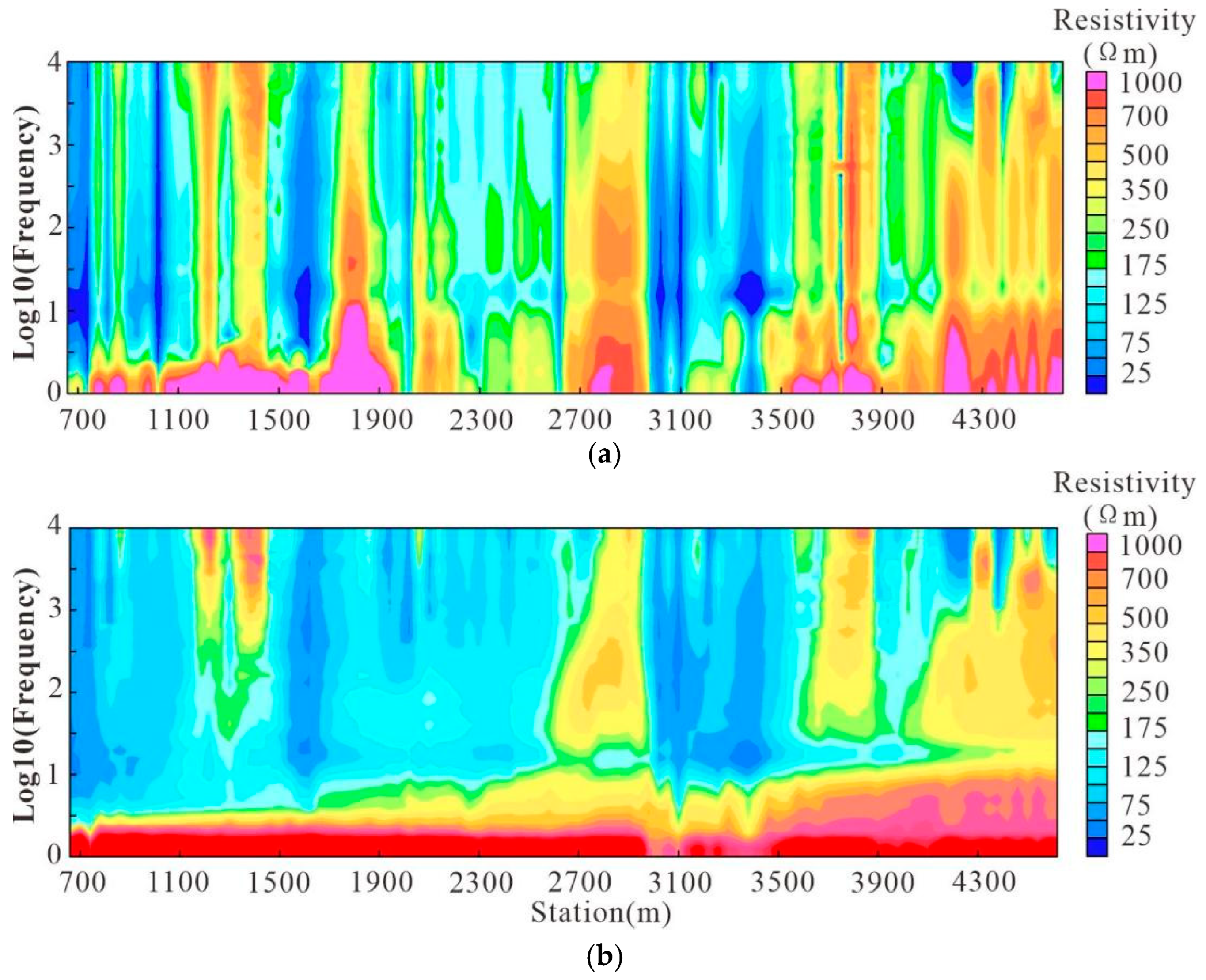
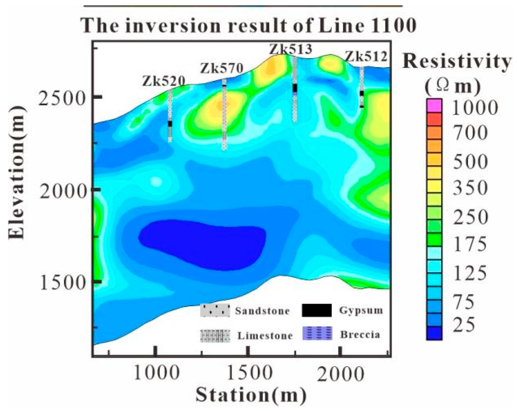
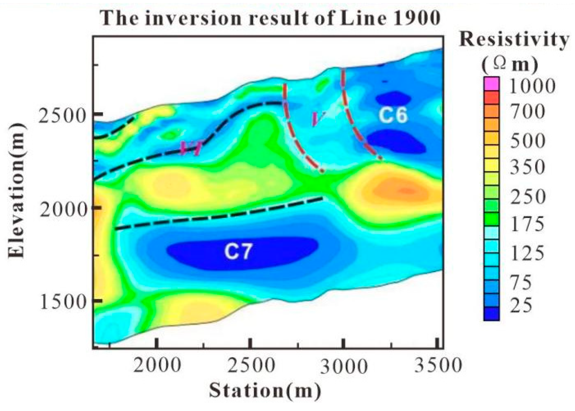
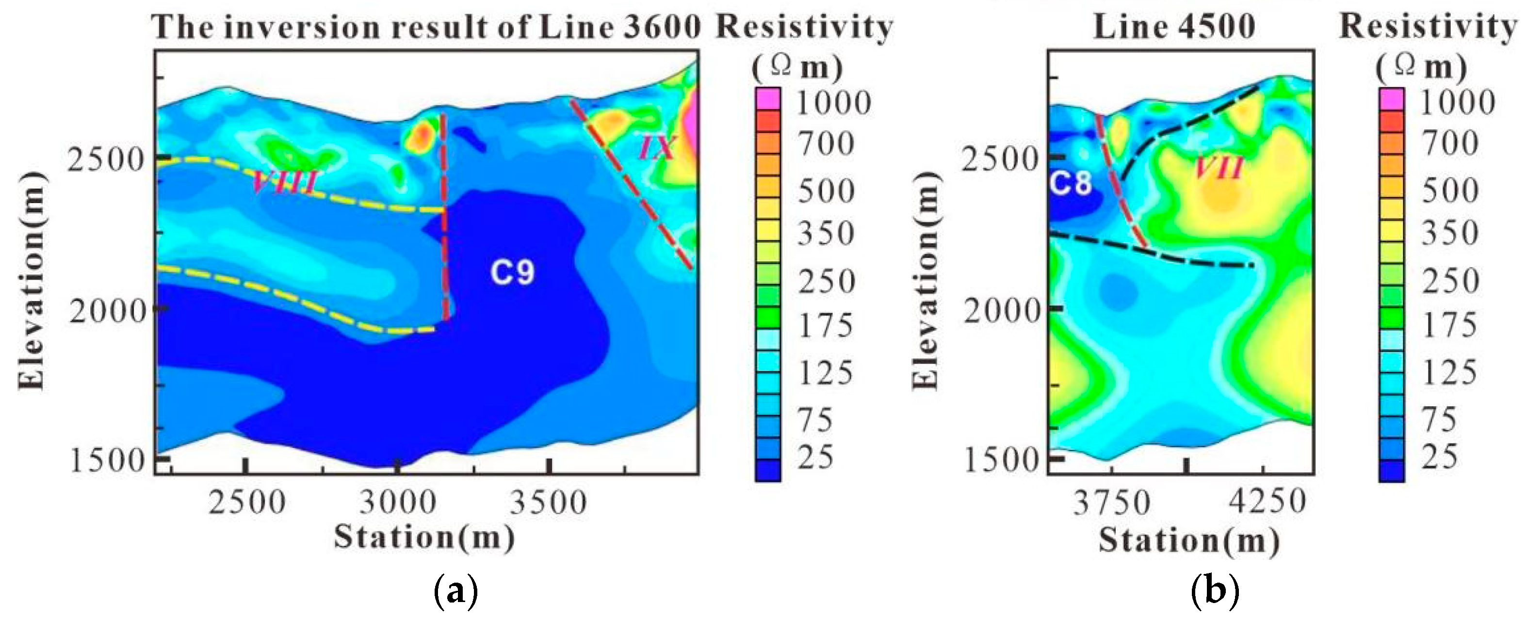
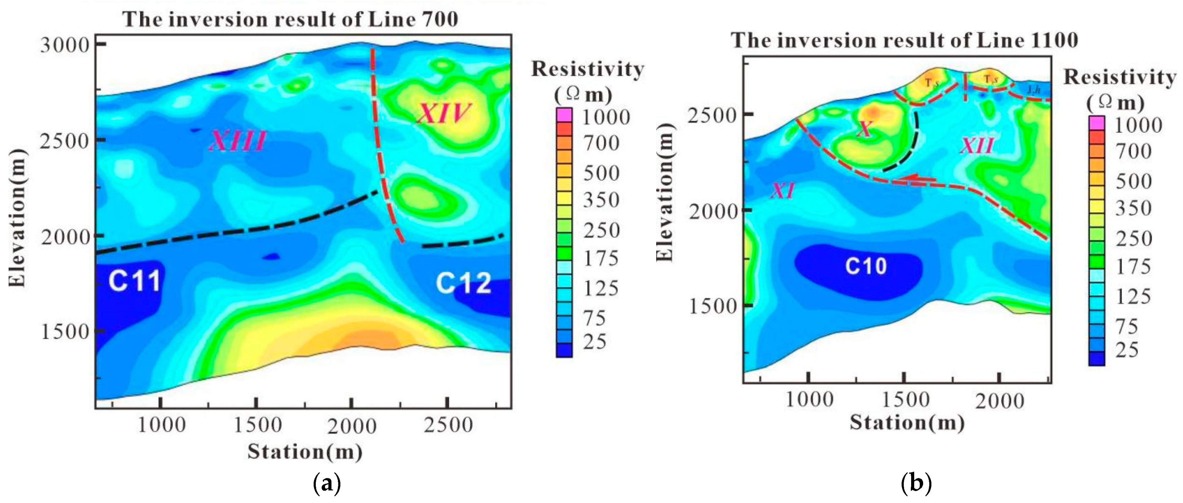
By using two-dimensional continuous medium inversion, the electrical distribution at a depth of 1 km below each survey line in the Jinding lead–zinc mining area was obtained. At the same time, by interpreting the electrical structure of the survey lines, the electrical characteristics of the lithologic system in the Jinding lead–zinc mining area were revealed. These results provide reliable data support for the geological genesis and metallogenic model of the Jinding lead–zinc deposit.

References

1. Gao, G. Review of Geological Origin about Jinding Lead-Zinc Ore Deposit. Earth Sci. 1989, 14, 468–475. [Google Scholar]
2. Qin, G.; Zhu, S. Genesis Model and Prospecting Prediction of the Jinding Lead-Zinc Deposit. Yunnan Geol. 1991, 10, 145–190. [Google Scholar]
3. Wang, G.; Hu, R.; Wang, C.; Zeng, Y.F. Mineralization Geological Setting of Jinding Super Large Pb-Zn Deposit, Yunnan. Acta Mineral. Sin. 2001, 21, 571–577. [Google Scholar] [CrossRef]
4. Yan, W.; Li, Z. Geochemical Characteristics and Hydrothermal Sedimentary Genesis of a New Type of Copper Deposit. Geochimica 1997, 1, 54–63. [Google Scholar] [CrossRef]
5. Zhu, Z.; Guo, F. Characteristics of Salt Structures and Links to Pb-Zn Mineralization of the Jinding Deposit in Lanping Basin, Western Yunnan. Geotecton. Metallog. 2016, 12, 201–204. [Google Scholar] [CrossRef]
6. Zhang, F.; Tang, J.; Fan, X.; Chen, H.; Chen, S.; Chen, W.; Wang, C.; Xie, H. A tentative discussion on mud diapiric fluid metallogenic characteristics of Jinding lead-zinc deposit in Lanping. Miner. Depos. 2010, 29, 361–370. [Google Scholar] [CrossRef]
7. Zeng, P.; Li, H.; Li, Y.; Wang, Z.; Wen, L.; Liu, S. Asia’s Largest Pb-Zn Deposit: The Jinding Giant Lead-Zinc Deposit Formed by Three-Stage Superimposed Mineralization. Acta Geol. Sin. 2016, 90, 2384–2398. [Google Scholar]
8. Zhang, F.; Tang, J.; Chen, H.; Fan, X.; Chen, S.; Chen, W.; Wang, C.; Xie, H. Evolution of the Lanping Basin and Characteristics of Metallogenic Fluids within the Basin. Acta Mineral. Sin. 2010, 30, 223–229. [Google Scholar]
9. Ma, S.; Li, W.; Li, W. Application of Geophysical Methods in the Jinding Area of Lanping. China Water Transp. 2019, 19, 181–182. [Google Scholar]
10. Gao, Y.; Liu, J.; Gao, Y.; Feng, X. Application of CSAMT in Looking for Hidden and Deep Mines. Northwestern Geol. 2010, 43, 135–142. [Google Scholar] [CrossRef]
11. Yu, C. The application of CSAMT method in looking for hidden gold mine. Chin. J. Geophys. 1998, 41, 133–138. [Google Scholar]
12. Wang, G.; Zhang, Z.; Li, Y.; Zhu, W.; Yao, D. The Method of Tensor CSAMT and Its Application Effects. Comput. Tech. Geophys. Geochem. Explor. 2016, 38, 598–602. [Google Scholar] [CrossRef]
13. Wu, L.; Li, Y. Application of CSAMT to the search for groundwater. Chin. J. Geophys. 1996, 39, 712–717. [Google Scholar] [CrossRef]
14. He, J. Wide field electromagnetic sounding methods. J. Cent. South Univ. (Sci. Technol.) 2010, 41, 1065–1072. [Google Scholar]
15. Jiang, X. 3D Modeling of Mines and Its Application Based on 3Dmine. Master’s Thesis, Kunming University of Science and Technology, Kunming, China, 2018; pp. 35–49. [Google Scholar] [CrossRef]
16. Tang, J.; Zhang, L.; Gong, J.; Xiao, X. 3D frequency domain controlled source electromagnetic numerical modeling with coupled finite element-infinite element method. J. Cent. South Univ. (Sci. Technol.) 2014, 45, 1251–1260. [Google Scholar]
17. Ren, Y.; Kalscheuer, T.; Greenhalgh, S.; Maurer, H. A goal-oriented adaptive finite-element approach for plane wave 3-D electromagnetic modelling. Geophys. J. Int. 2012, 194, 700–718. [Google Scholar] [CrossRef]
18. Ren, Y.; Kalscheuer, T.; Greenhalgh, S.; Maurer, H. A finite-element-based domain- decomposition approach for plane wave 3D electromagnetic modeling. Geophysics 2014, 201, 255–268. [Google Scholar] [CrossRef]
19. Yonghyun, C.; Son, J.; Lee, T.; Kim, H.J.; Shin, C. Three-dimensional modelling of controlled-source electromagnetic surveys using an edge finite-element method with a direct solver. Geophys. Prospect. 2014, 62, 1468–1483. [Google Scholar] [CrossRef]
20. Yin, C.; Ben, F.; Liu, Y.; Huang, W.; Cai, J. MCSEM 3D modeling for arbitrarily anisotropic media. Chin. J. Geophys. (Chin.) 2014, 57, 4110–4122. [Google Scholar] [CrossRef]
21. Castillo-Reyes, O.; Puente, J.; Puzyrev, V.; Cela Espín, J.M. Edge-based electric field formulation in 3D CSEM simulations: A parallel approach. In Proceedings of the 2015 International Conference and Workshop on Computing and Communication (IEMCON), Vancouver, BC, Canada, 15–17 October 2015. [Google Scholar] [CrossRef]
22. Huang, W.; Yin, C.; Ben, F.; Liu, Y.; Chen, H.; Cai, J. 3D Forward Modeling for Frequency AEM by Vector Finite Element. Earth Sci. 2016, 41, 331–342. [Google Scholar] [CrossRef]
23. Gratkowski, S.; Ziolkowski, M. A three-dimensional infinite element for modeling open-boundary field problems. IEEE Trans. Magn. 1992, 28, 1675–1678. [Google Scholar] [CrossRef]
24. Gratkowski, S.; Ziolkowski, M. On the accuracy of a 3-D infinite element for open boundary electromagnetic field analysis. Arch. Fur Elektrotechnik 1994, 77, 77–83. [Google Scholar] [CrossRef]
25. Gong, J. Application of Finite Element-Infinite Element Coupling Method on 3D Electric and Electromagnetic Numerical Modeling. Master’s Thesis, Central South University, Changsha, China, 2009. [Google Scholar] [CrossRef]
26. Vozoff, K. Electromagnetic methods in applied geophysics. Geophys. Surv. 1980, 4, 9–29. [Google Scholar] [CrossRef]
27. Korotaev, S.M.; Zhdanov, M.S.; Orekhova, D.A.; Kruglyakov, M.S.; Trofimov, I.L.; Schors, Y.G.; Shneyer, V.S. Study of the possibility of the use of the magnetotelluric sounding method in the Arctic ocean with quantitative modeling. Izv. Phys. Solid Earth 2010, 46, 759–771. [Google Scholar] [CrossRef]
28. Jin, J.M. The Finite Element Method in Electromagnetics; John Wiley & Sons: Hoboken, NJ, USA, 2014. [Google Scholar]
29. Astley, R.J.; Macaulay, G.J.; Coyette, J.P. Mapped Wave Envelope Elements for Acoustical Radiation and Scattering. J. Sound Vib. 1994, 170, 97–118. [Google Scholar] [CrossRef]
30. Dai, S.; Xu, S. Rapid inversion of MT date for 2-D and 3-D continuous media. Oil Geophys. Prospect. 1997, 32, 305–317. [Google Scholar] [CrossRef]
31. Su, Q.; Dai, S.; Zhao, D. Modeling and inversion of the CSEM field in 2.5D anisotropic media with an adaptive finite element method. Oil Geophys. Prospect. 2018, 53, 418–429. [Google Scholar] [CrossRef]
Figure 1. Simplified geological map of the Jinding mining area, Yunnan Province.
Applsci 15 04303 g001
Figure 2. Two-dimensional geological model of the Jinding lead–zinc deposit.
Applsci 15 04303 g002
Figure 3. Three-dimensional geophysical model of the Jinding lead–zinc deposit.
Applsci 15 04303 g003
Figure 4. Calculation domain of the finite and infinite element.
Applsci 15 04303 g004
Figure 5. Mapping of the finite element. (a) Sub element; (b) parent element.
Applsci 15 04303 g005
Figure 6. Mapping of the infinite element. (a) Sub element; (b) parent element.
Applsci 15 04303 g006
Figure 7. Cagniard apparent resistivity pseudo-section view of the geophysical model.
Applsci 15 04303 g007
Figure 8. Comparison of the amplitude between the noise and total signals at the test point. (a) Amplitude of the noise signal in E; (b) amplitude of the noise signal in H; (c) amplitude of the total signal in E; (d) amplitude of the total signal in H.
Applsci 15 04303 g008
Figure 9. SNR curve for (a) magnetic fields and (b) electric fields at the test point.
Applsci 15 04303 g009
Figure 10. Comparison of apparent resistivity sounding curves at different collection times.
Applsci 15 04303 g010
Figure 11. Curve diagrams of apparent resistivity sounding at certain survey points.
Applsci 15 04303 g011
Figure 12. Pseudo-section diagram of CSAMT apparent resistivity for Line 2100. (a) Original pseudo-section diagram; (b) pseudo-section diagram after static correction.
Applsci 15 04303 g012
Figure 13. Comparison of the shallow electrical structure with the physical properties of drill core data for Line 1100.
Applsci 15 04303 g013
Figure 14. Location of Line 2400’s survey line and its electrical structure profile.
Applsci 15 04303 g014
Figure 15. Location of Line 2100 and its electrical structure profile.
Applsci 15 04303 g015
Figure 16. Location of Line 1900 and its electrical structure profile.
Applsci 15 04303 g016
Figure 17. Location of (a) Line 3600 and (b) Line 4500 and their electrical structure profiles.
Applsci 15 04303 g017
Figure 18. Location of (a) Line 700 and (b) Line 1100 and their electrical structure profiles.
Applsci 15 04303 g018