Experimental Investigation into the Number of Phases in Debris Flows

Abstract

Controversial number of phases in debris-flow masses involves almost all areas of debris-flow research. In this study, we experimentally investigated the number of phases in fully developed debris flows using six sediments with three maximum diameters of up to 30 mm from two representative debris-flow deposits in China. Fluid escape tests, displacement experiments, relative motion experiments, and rheometrical tests were conducted using 12 slurries prepared with the sediments. The results from four types of experiments show that debris flows are close to one-phase flow and far from two-phase flow. Under both gravity and artificial hydraulic and mechanical forcing, no relative motion of water or fluid composed of water and fine-grained particles and solids occurs in both the experimental flows and static slurries. This suggests that the water and solids in debris flows move together as a single fluid, and are deposited by “freezing”. The rheological behavior of the experimental debris flows is similar to that of Bingham materials. This indicates that debris flows may be approximated as continuous, homogeneous, isotropic fluids. In conclusion, debris flows behave more like monophasic flow, are far from biphasic flow, and should be treated as one- rather than as two-phase flow.

1. Introduction

Debris flows [1,2,3] are known to be mixtures of water and poorly sorted sediments that advance downstream channels or hillslopes. However, this does not define the full range of debris-flow characteristics. Many exciting fields of research remain to be thoroughly explored despite the major advancements made in debris-flow studies over the past 100 years, and the number of phases in debris-flow bodies is an important problem that is yet to be investigated in detail.

Researchers studying debris flows have traditionally espoused two major opinions on this disputed topic: one-phase (single-phase or mono-phase) and two-phase flows. The one-phase theory [4,5,6,7,8] emphasizes that debris flows can be considered as homogeneous yield-stress fluids [9,10,11]. The two-phase hypothesis argues that debris flows consist of fluid and solid fractions and stresses the importance of fluid and its interaction with solids [12,13,14,15].

The difference in the understanding of debris flow between the two hypotheses is significant. The former considers that the combination of water and solids results in a new material in which they move together and are deposited en masse, whereas the latter considers fluid and fluid–solid interactions to be important. The most important discrepancy between the two views is whether the relative motion of fluid and solids occurs in debris flows.

Perhaps some debris flows can superficially appear as two-phase flow, but an irretrievable question of the two-phase assumption is how to distinguish between the solid and fluid components of debris flows, or what constitutes the fluid fraction. The grain-size thresholds separating the sediment belonging to the solid or the fluid phase used in the literature include clean water (i.e., pure fluid or interstitial fluid with a negligible amount of fine solid fraction) [16,17,18,19], 0.002 mm (clay size [20,21]), 0.0625 mm (sand–silt boundary size [22,23,24]), 0.1 mm [25], 2 mm (sand size [12,26]), ~6 mm [24], and 20 mm [26].

These widely ranging threshold grain sizes (spanning over four orders of magnitude) would seem to indicate the absence of “solid phase” in debris flow, because this threshold can be reasonably extrapolated to 30 mm, 40 mm, and up to boulders (>75 mm in diameter) [21], as long as gradation is continuous (which is the case for typical debris-flow materials [12,20]). Thus, debris flows including boulders [7,27,28,29,30] are behaving as “fluid”. In other words, the high variability in the boundary size that distinguishes fluids and solids indirectly justifies the one-phase view to some degree.

The number of phases used by investigators dealing with debris flows remains a major concern because it directly influences the identification of debris flows and their deposits, description of kinematics and dynamics, and assessment of geomorphological and hazardous effects [2,31,32,33,34].

An inadequate understanding of the number of phases in debris flows is due to a lack of experimental evidence. Here, we experimentally investigate the number of phases within debris-flow masses using the representative sandy (granular, stony, or boulder [24,35,36,37]) and muddy [26,38,39,40,41] debris-flow materials in China. In addition, only fully developed debris flows (slurry flows [42]) constituting the body between the head and tail of surges (pulses) (Figure 13.6 in Pierson (1986) [43]; Figure 10F in Eger et al. (2018) [36]), that is, the main body of debris flows (hereafter referred to as debris flows), were involved in this study.

2. Sampling Sites

The sandy–silt debris-flow sample [44] used in this study is collected from the well-preserved debris flow deposit (27°38′21.31″ N, 98°44′4.74″, Figure 1 in Ye et al. (2024) [45]) about 500 m upstream of the Dongyuege (DYG) Creek (a tributary to the Nu River) fan. The DYG event, which occurred on 18 August 2010, was typical of Nu River debris flows. The Nu River catchment area is the most prone to sudden and catastrophic debris flows, in China.

Geologically, the Nu River catchment is hosted in the N–S extensional Nu River fault zone, which is ~500 km long and 20–30 km wide in Yunnan, China, and is dominated by medium- to high-grade metamorphic rocks [46]. The strong downcutting of the Nu River and its hundreds of tributaries, driven by the uplift of the Tibetan Plateau in the Cenozoic, and abundant loose sediment fed highly fragmented bedrock, preconditioned a multitude of debris-flow-producing basins.

The DYG debris flow has the following characteristics: high magnitude [35,47], high elevation of the initiation area [48] and large relief of the flow track, long reach, high mobility, and high competence [45,49,50,51,52,53].

(ⅰ) Approximately 6 × 10⁵ m³ of sediment was delivered to the alluvial fan, killing 96 people. (ⅱ) The event initiated at elevations of 3000–3500 m a.s.l., near the snow line, whereas the fan ranges in elevation from 1400 m to 1450 m a.s.l. (ⅲ) Its total travel and runout distances [12,39,54] reached 11 km and 9 km, respectively. (ⅳ) It traveled up to 3.3 km in a low-gradient channel (2°–5°) upstream of the mouth of the DYG Creek. (ⅴ) Three large boulders, 7–9 m in size, were transferred from the stream channel ~8 km upstream of the fan apex onto the fan in addition to common boulders of many tens of centimeters in the deposits. (ⅵ) The <0.005 mm fraction of the deposit contained no typical clay minerals [21,55], and the plasticity index of the <0.075 mm fraction was only 6.9, which was governed by basin bedrock composed predominantly of granite, schist, gneiss, quartzite, and marble.

The DYG event is representative of common alpine debris flows [39,56,57], with a predominant sandy silt texture.

The Jiangjia Gully (JJG) debris flow (26°14′50.65″ N, 103° 8′4.57″ E, Figure 1 in Ye et al. (2024) [45]) sampled in this study is known for extreme debris-flow activity and has received the most intensive study [4,6,28,29,37,58], especially in China [59,60,61,62,63,64,65,66,67,68]. As expected, the magnitude of the JJG flow was relatively low, with the sediment mobilized by a single surge commonly having volumes of thousands of m³ to tens of thousands of m³. It is interesting to note that the largest clasts in the JJG debris-flow deposits rarely have a maximum dimension of greater than 0.5 m (generally <0.3 m). This phenomenon can be ascribed to bedrock geological controls, that is, lithological and structural predisposition. The JJG basin is underlain by highly fragmented Proterozoic slate and is also part of the active Xiao River fault zone, which is of regional importance and is several kilometers wide and ~350 km long. The Xiao River watershed has an area of approximately 2950 km², is preconfigured by the fault zone, and has been repeatedly subjected to debris flows.

Profoundly different from the DYG flow, the <0.005 mm fractions of the JJG debris-flow deposit are dominated by typical clay mineral (illite), and the plasticity indices of the <0.5 mm and <0.075 mm fractions can reach 12.0 and 12.4, respectively [52,53]. Therefore, the JJG deposits can be thought of as the product of muddy debris flows [26,38,39,40].

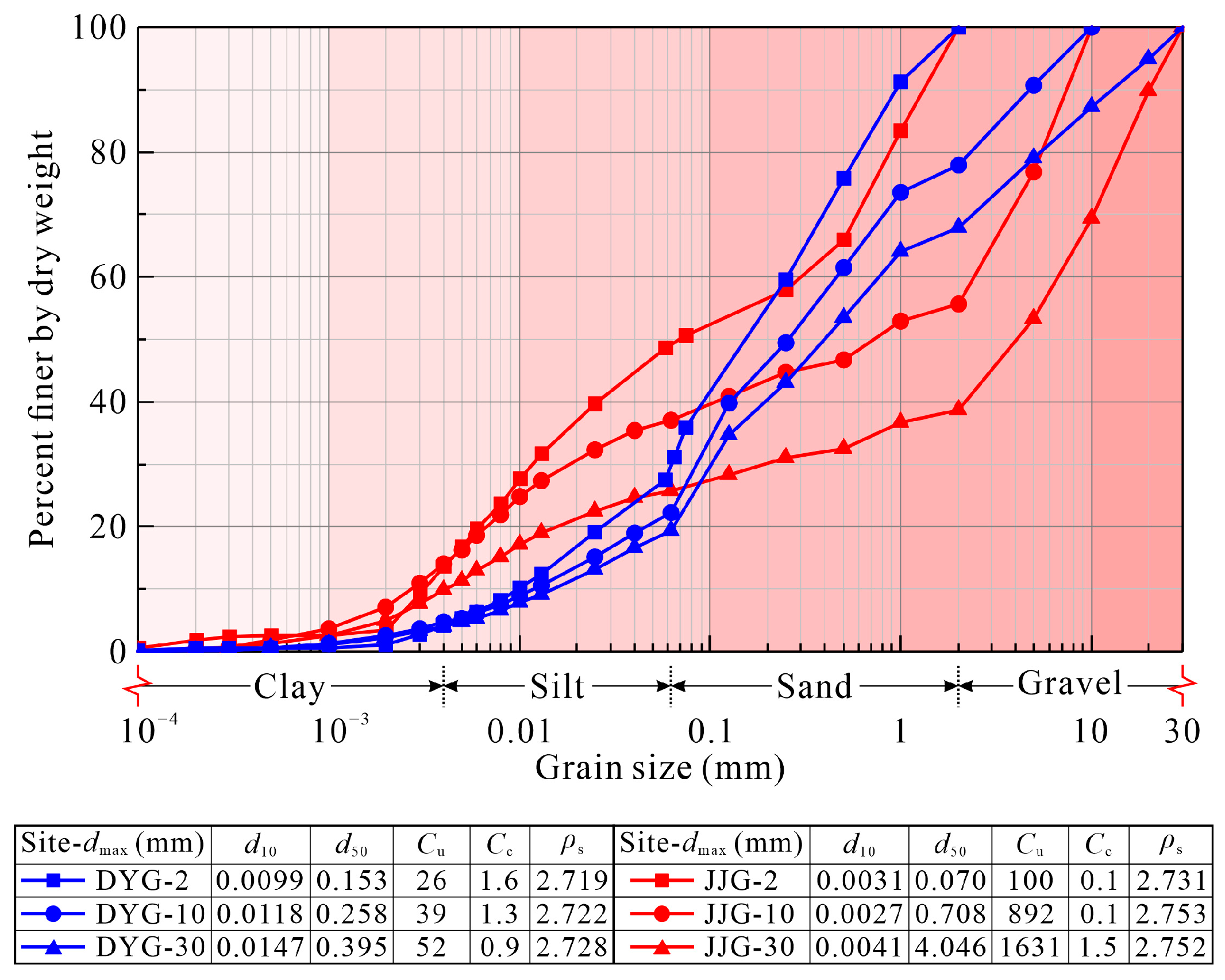
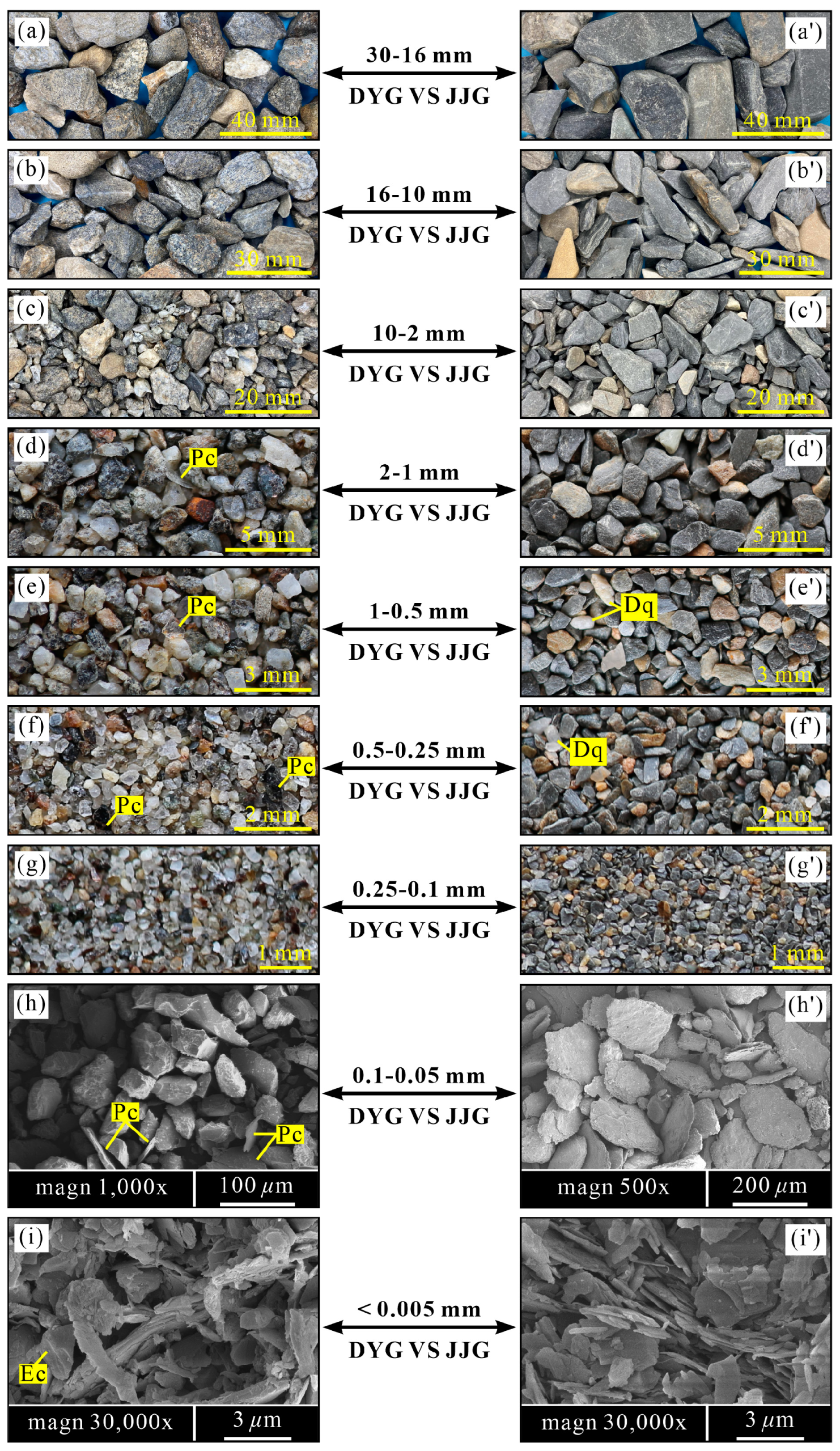
3. Tested Clastic Materials

For each of the two debris-flow deposits, three clastic materials with maximum grain diameters (d_max) of 2, 10, and 30 mm were prepared by sieving the large bulk samples up to 100 mm in diameter stored in the laboratory (which were collected during the sampling campaigns carried out at the DYG in November 2015 and November 2019 and JJG in March 2017, respectively (Ye et al. (2024) [45])). The grain-size distributions of six materials, determined using wet sieving coupled with laser granulometry (for <0.025 mm fraction) (using a laser particle-size analyzer, Beckman Coulter^®LS 13320) (Beckman Coulter, Brea, CA, USA), are shown in Figure 1.

C_u and C_c show that both tested materials are very poorly to extremely poorly sorted and are typical of debris-flow deposits [2,9,20,33,69,70,71]. The distinction in particle size distribution (characterized by C_u and C_c) between the DYG and JJG clasts of the same d_max is also obvious; the former shows a more continuous gradation than the latter.

Furthermore, the materials from the two sites differed significantly in terms of debris geometry. The eight size fractions (ranging from 30 mm to 0.05 mm) of the DYG debris consisted mainly of equidimensional clasts (Figure 2a–h) derived from granite, schist, gneiss, and monocrystalline quartz. Platy/flaky clasts of muscovite and biotite that could be identified using megascopic methods (Figure 2d–f) or through a scanning electron microscopy (SEM) (Figure 2h) were frequently observed in relatively fine-grained particles. Perhaps due to the limitations of the adopted separation method, the <0.005 mm fraction of the DYG deposit was limited almost entirely to platy/flaky detrital mica, with occasional equidimensional grains (Figure 2i).

Figure 1. Grain-size curves of six clastic materials up to 30 mm in diameter (d_max), separated from the DYG and JJG debris-flow deposits. d₁₀ and d₅₀ are effective grain size and average grain size, respectively. C_u and C_c are coefficient of uniformity and coefficient of curvature, respectively [21]. ρ_s is solid density (grain density) (g/cm³), which is determined using the methods described in GB/T 50123-2019 [72].

Figure 1. Grain-size curves of six clastic materials up to 30 mm in diameter (d_max), separated from the DYG and JJG debris-flow deposits. d₁₀ and d₅₀ are effective grain size and average grain size, respectively. C_u and C_c are coefficient of uniformity and coefficient of curvature, respectively [21]. ρ_s is solid density (grain density) (g/cm³), which is determined using the methods described in GB/T 50123-2019 [72].

Figure 2. Distinct shapes of the tested DYG ((a–i), equidimensional) and JJG ((a′–i′), platy/flaky) debris (eight size fractions of >0.05 mm), and their platy/flaky fines (<0.005 mm fraction). Ec, equidimensional clasts. Pc, platy clasts (mica). Dq, detrital quartz.

Figure 2. Distinct shapes of the tested DYG ((a–i), equidimensional) and JJG ((a′–i′), platy/flaky) debris (eight size fractions of >0.05 mm), and their platy/flaky fines (<0.005 mm fraction). Ec, equidimensional clasts. Pc, platy clasts (mica). Dq, detrital quartz.

In contrast, the platy/flaky clasts dominated the JJG debris. The 30–0.05 mm fraction of the JJG debris was composed almost exclusively of platy/flaky or lenticular clasts of slate (Figure 2a′–h′), and equidimensional grains (quartz) were infrequently observed (Figure 2e′,f′). The platy/flaky detrital mineral (illite) comprises nearly the entire <0.005 mm fraction of this material (Figure 2i′).

The striking contrast between the grain geometries of the DYG and JJG debris can be ascribed to the aforementioned differences in the bedrock lithologies underlying the two basins.

In short, the DYG debris is dominated by equidimensional clasts and has continuous gradation, whereas the JJG debris consists of platy/flaky clasts with less continuous gradation.

In summary, the DYG and JJG flows represent two common debris-flow types: sandy and muddy [4,29], respectively. Their debris is dominated by equidimensional and platy/flaky clasts, which typify the two end-members of the geometry of clasts [21] that compose debris flows. The experimental results obtained for these two deposits are representative of other debris flows.

4. Laboratory Experiments

According to the lower limit of solid volume concentration (C_v) for slurrying (${\mathrm{C}}_{\mathrm{v}}^{\mathrm{h}}$, boundary C_v between debris flow and hyperconcentrated flow [7,9,22,73]) and debris-flow index (I_d) of sediments [49], two sediment–water mixtures (slurries) with different C_v (approximately ${\mathrm{C}}_{\mathrm{v}}^{\mathrm{h}}$ + 0.33I_d and ${\mathrm{C}}_{\mathrm{v}}^{\mathrm{h}}$ + 0.66I_d, respectively) are prepared for each of the six debris-flow materials shown in Figure 1, to assess the reproducibility of the experimental results. The properties of the 12 experimental slurries are listed in

Table 1. Properties of the 12 experimental slurries.

Slurry Number	Debris Source	dmax (mm)	Cv	ρb (g/cm3)	w (wt.%)
DYG-2-0.55	DYG	2	0.55	1.95	23.2
DYG-2-0.57			0.57	1.98	22.2
DYG-10-0.60		10	0.60	2.04	19.5
DYG-10-0.62			0.62	2.07	18.4
DYG-30-0.64		30	0.64	2.11	16.9
DYG-30-0.66			0.66	2.14	15.9
JJG-2-0.53	JJG	2	0.53	1.91	25.4
JJG-2-0.54			0.54	1.94	24.2
JJG-10-0.60		10	0.60	2.05	19.5
JJG-10-0.62			0.62	2.09	18.2
JJG-30-0.68		30	0.68	2.19	14.5
JJG-30-0.70			0.70	2.23	13.5

w (water content) = [(weight of water)/(weight of water + solids)] × 100. ρ_b is bulk density of the slurry. C_v (solid volume concentration) = (volume of solids)/(volume of water + solids).

.

An investigation into the number of phases in debris flows is performed by determining whether the relative motion of fluid and solids can occur in them; that is, by examining the presence or absence of fluid capable of moving independently of solids. To this end, four independent experiments, capable of mutually verifying each other, were conducted on each of the 12 slurries shown in Table 1, considering the potential influences of clast composition [69] (including grain-size distribution and clast geometry), d_max, and C_v.

4.1. Escape Test of Fluid

An escape test of fluid is similar to a slump one [40,74,75], and, to a lesser extent, to a dam-break one [26,39,76]. It was intended to investigate the differentiated responses of potential fluid and solid phases to the sudden release of the slurry.

The escape test was run by abruptly lifting cylindrical containers holding the slurry on a gently tilted smooth surface with an inclination of 5°, which corresponds roughly to the surface gradients of debris-flow fans, that is, the deposition angles of debris flows [20,39,71,77], and can assist the relative motion of fluid and solids (if present). The diameters of the two containers used were 10 (for eight slurries with d_max = 2 and 10 mm) and 30 cm (for four slurries with d_max = 30 mm), and their respective heights were 4.3 and 11.5 cm, which, on the inclined plane, produced storage volumes (V) of 300 and 7170 cm³, respectively.

The experimental flow propagation on the tilting plane was observed and recorded. After full stoppage of runout, we photographed experimental deposits (to take orthophotos), capturing their three-dimensional geometry with a 3-D laser scanner (Leica^®Scan Station C10) (Leica, Wetzlar, Germany), collected and weighed the fluid (effluents) escaping out of main deposits (if there was any), and determined the grain-size distribution of sediments constituting the effluents with the laser diffraction particle size analyzer described above.

The uniformity of runout is characterized by coefficient of runout (C_r). C_r is defined as the ratio of the surface area including the convex sides (A_s) to the inundated area [7,34,54,76,78,79,80] of deposits (A_i),

$$C_{\mathrm{r}}={\displaystyle \frac{A_{\mathrm{s}}}{A_{\mathrm{i}}}}$$

(1)

Additionally, Solidity (S) was used to describe the 2-D geometry of the experimental deposits and was defined as A_i divided by the area of the minimum circumscribed polygon of the deposits. As the irregularities at the boundary of a deposit decrease, S increases to a maximum value of 1.

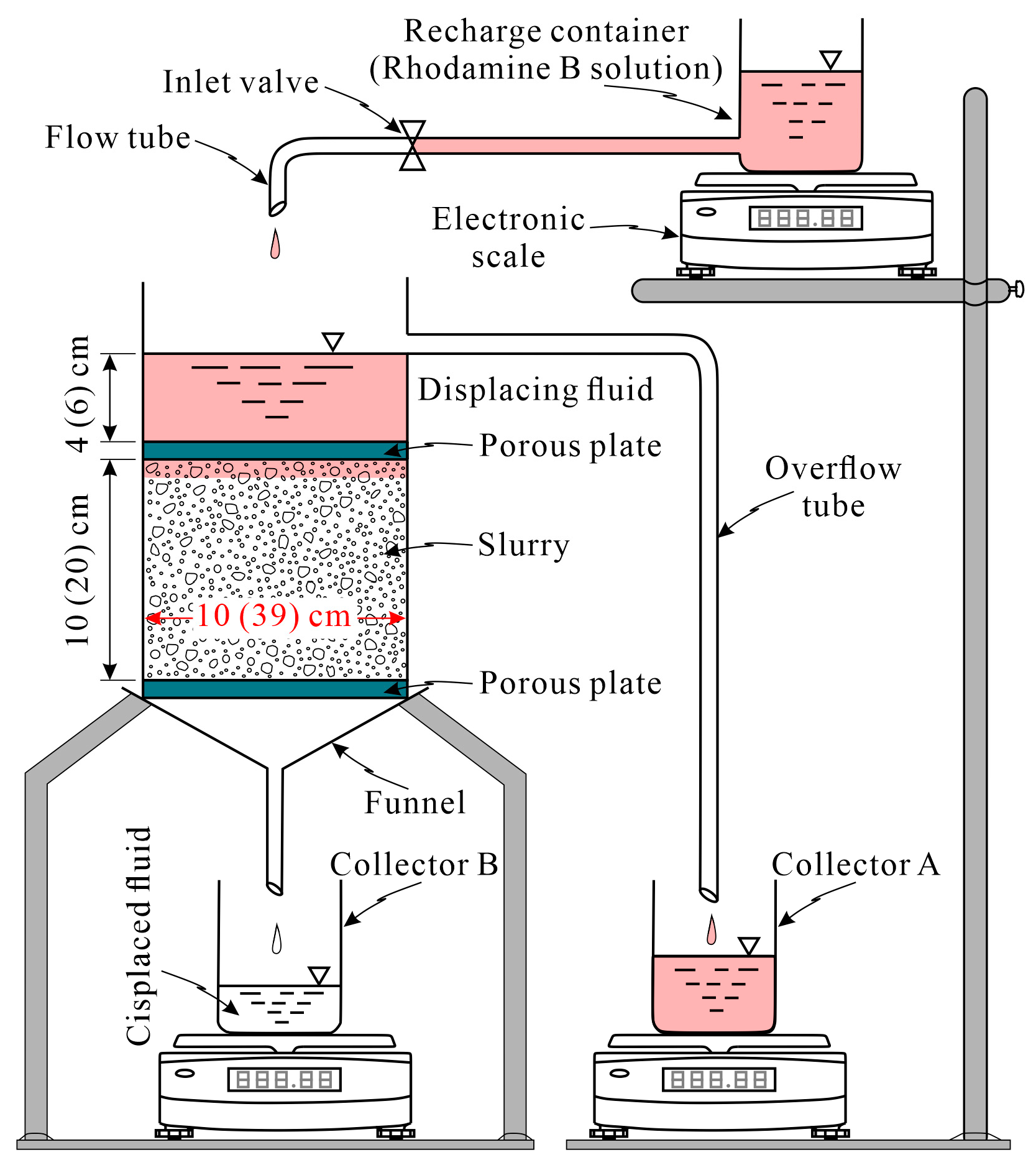
4.2. Displacement Experiment of Fluid (Water) Under Constant-Head Condition

To further investigate the potential for the relative motion of fluid and solids in debris flows, we conducted displacement experiments [81], which were run by displacing the fluid (water) in the experimental slurries with (red) Rhodamine B solution under constant-head conditions [76,82,83,84] (Figure 3).

The tested slurry columns of two sizes, contained in PVC cells, stood 10 cm (for the slurries of d_max = 2 and 10 mm) and 20 cm (for the slurries of d_max = 30 mm) (H) tall with respective diameters of 10 and 39 cm, and respective constant cross-sectional areas (A) of ~79 and ~1195 cm². They were overlain by 4 and 6 cm high Rhodamine B solution (serving as displacing fluid [85]) columns, respectively, which were maintained using the recharge container and collector A for overflow placed on electronic scales. Therefore, constant hydraulic gradients (J) of 1.4 and 1.3 were established within the slurries with the two different d_max values. The fluid (water) displaced from the slurry column (effluent) was captured below the lower end of the column using collector B, which was placed on an electronic scale.

The temporal color changes and cumulative quantity of effluent (displaced fluid) (converting weight to volume by assuming that the density of water is 1 g/cm³) (V_we), and the cumulative quantity of the injected Rhodamine B solution (displacing fluid) (the difference between the quantity in the recharge container and collector A) (V_wd) were measured at 5 min intervals throughout the 600 min testing period.

Using the obtained measurements, the percentages of V_we and V_wd in the initial amount of water contained in the tested slurry (V_wi) (P_e and P_d) were derived as follows:

$$P_{\mathrm{e}}={\displaystyle \frac{V_{\mathrm{we}}}{V_{\mathrm{wi}}}}\times 100\%$$

(2)

$$P_{\mathrm{d}}={\displaystyle \frac{V_{\mathrm{wd}}}{V_{\mathrm{wi}}}}\times 100\%$$

(3)

The potential for the relative motion of fluids and solids is characterized by the displacement ratio (DR). DR is defined as the percentage of the volume of water displaced from a unit slurry volume (i.e., representative elementary volume, REV [82]) under a unit hydraulic gradient (J) relative to that originally contained in the REV.

$$DR={\displaystyle \frac{V_{\mathrm{we}}}{A\times H\times (1-C_{\mathrm{v}})\times J}}\times 100\%$$

(4)

$$DR={\displaystyle \frac{V_{\mathrm{we}}}{V_{\mathrm{wi}}\times J}}\times 100\%={\displaystyle \frac{P_{\mathrm{e}}}{J}}$$

(5)

Thus, for each of the 12 slurries (Table 1), the time series of P_e, P_d, and DR were obtained.

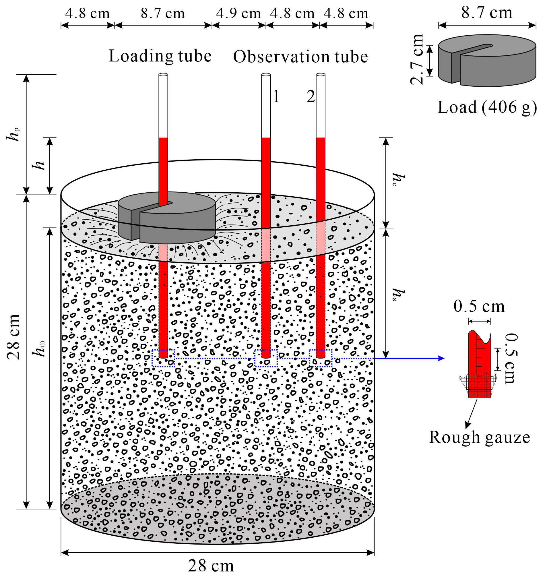
4.3. Relative Motion Experiment of Fluid (Water) and Solids Under Load

In this experiment, we attempted to evaluate the relative motion of fluids (water) and solids within debris-flow masses by examining the hydraulic connections between different locations (or representative elementary volume [82]) in the experimental slurries under externally applied loads.

A relative motion experiment was conducted in a cylindrical stainless-steel storage container (28 cm tall, 28 cm in diameter, and approximately 17 L (L)) (Figure 4). The height of the slurry column was 26 cm. All test runs, which were distinguished by modifying the experimental debris (source and d_max), solid volume concentrations (Table 1), and measured depths were performed using a bulk volume of approximately 16 L.

After the slurry was poured into the container, three graduated piezometers with an inner diameter of 5 mm and a gauze-screened bottom end (inlet) arranged along the diameter of the bucket (from left to right, the loading tube and observation tubes 1 and 2) were quickly inserted vertically into the slurries to predetermined depths (the initial value of the hydrostatic pressure (h_s0)) of 6, 9, and 12 cm. Each of the 12 slurries listed in Table 1 was tested thrice to measure the water pressures at various depths. A total of 36 experimental runs were conducted.

Upon insertion, Rhodamine B solution was injected into the three piezometer tubes to a height of approximately 0.6 times h_s0 above the slurry surface (the initial value of excess water pressure, h_e0). Following the injection, the timing began, and the piezometric (or hydraulic) head, the elevation of the piezometers (h and h_p, measured with respect to the edge of the bucket), elevation of the surface of slurry (h_m) around the piezometers measured from the bottom of the bucket, excess water pressure (h_e), and hydrostatic pressure (h_s) (Figure 4) were continuously recorded at 5 min (for 0–180 min) and 10 min (for 180–600 min) intervals.

In this process, the free water escaping from the slurry onto its surface was collected using a pipette in a special beaker, and the corresponding weight increase of the water in the beaker was recorded while measuring the data listed above.

For virtually all three piezometers in all experimental runs, slow increases in h levels after injection to their peaks were observed, followed by a gradual drop. By trial-and-error iteration, a 406 g stony weight (87 mm in diameter and 27 mm thick) was gently placed on the slurry surface around the loading tube (Figure 4) 90 min after timing when h was approaching its peak. This was regarded as the application of an external surface load surrounding the piezometer.

For each of the 36 runs, the time series of h, h_p, h_m, and the relative excess water pressure (R = h_e/h_s) from the three piezometers, as well as the percentage of the cumulative discharge (PCD) of water in the initial amount of water in the tested slurry, were acquired over a monitoring period of 600 min.

4.4. Rheometrical Test of Bulk Behavior of Experimental Debris Flow

Rheometric tests (flow experiments) [4,10,26,30,73,86,87,88] were conducted to check the coherency of the moving debris-flow slurry, that is, the possibility that water and solids flow as a whole.

The rheology of eight slurries consisting of ≤2 and ≤10 mm sediments (Figure 1 and Figure 2, and Table 1) was measured using an Andon Paar MCR 52 rotational rheometer. The container of the rheometer was a thin-walled stainless-steel bucket with a diameter of 115 mm and height of 48 mm, filled with a slurry volume of ~500 mL. An eccentrically rotating sphere with a diameter of 15 mm fixed onto a thin holder was dragged through the slurries at variable rotational speeds [10] when the system functioned. The test was conducted by measuring the shear stress under an applied strain rate that was increased from 0 s⁻¹ to 30 s⁻¹ in 120 s, considering the typical shear rates for debris flows [7,28,89].

Four experimental debris flows with d_max = 30 mm were tested using a large-scale two-point type rheometer [30,74,75,90]. Its container (lined with a 13 mm grid wire mesh to avoid wall slip) had an inner diameter of 39.4 cm and a useful depth of 36.5 cm, which corresponded to a storage volume of ~45 L. The H impeller was 17 cm wide and 15 cm high. The distance between the impeller and the wire mesh was 11.2 cm, and that between the impeller and the container bottom was 10 cm.

5. Results

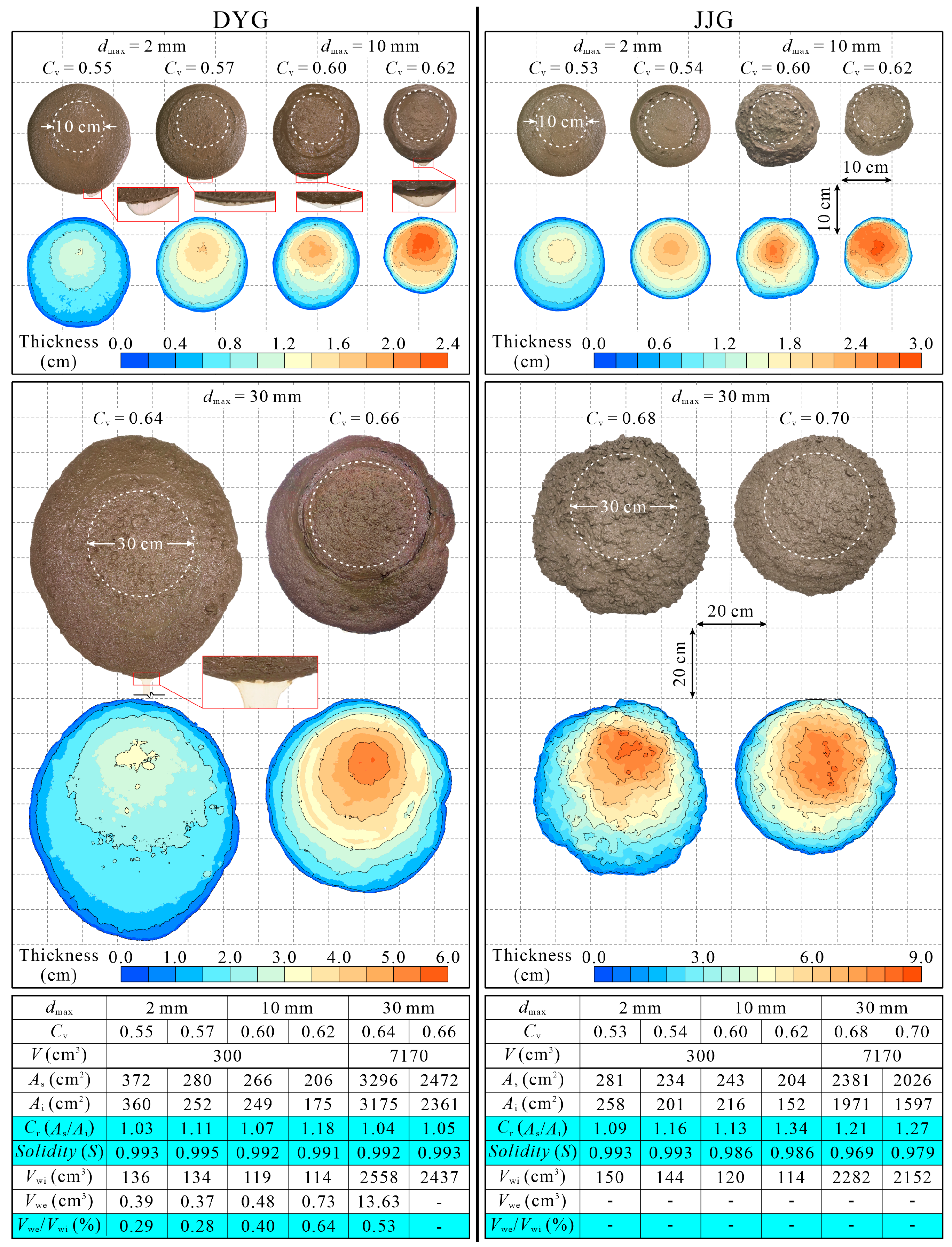
5.1. Escape of Fluid from Experimental Debris-Flow Deposits

The test results for the escape of the potential fluid from the experimental debris flows are shown in Figure 5. The orthophotos of the deposits and the initial positions of the slurry columns marked on the photos display the relatively high mobility of the tested slurries and the regular morphology of their deposits.

The measured C_r ranged from 1.03 to 1.27 with an average of 1.14. Twelve Solidity (S) values varied over a very narrow range (0.969–0.995), and the heights of distinguishable, irregular protrudes occurring only on the boundaries of the deposits with d_max = 30 mm were significantly smaller than 30 mm.

Six pairs of deposits of the same debris source and d_max exhibited a negative correlation between A_i (inundated area) and C_v (solid volume concentration) and a positive relationship between C_r (coefficient of runout) and C_v. This indicates that the measurements of the deposit geometry were reasonable to some degree.

No escape of fluid occurred in any of the three pairs of deposits composed of the JJG debris and DYG-30-0.66 (Table 1, Figure 5). The remaining five deposits did release some fluid, but the fluid collected within 60 min after full stoppage of runout (V_we) accounted for only 0.28–0.64% of the initial amount of water in their respective parent slurries (V_wi), with an average of 0.43%. In other words, V_we was negligible compared to V_wi. In addition, the fluid leaving the main deposits was essentially clear water (its solid (fines) concentration was below the detection limit of the laser particle size analyzer).

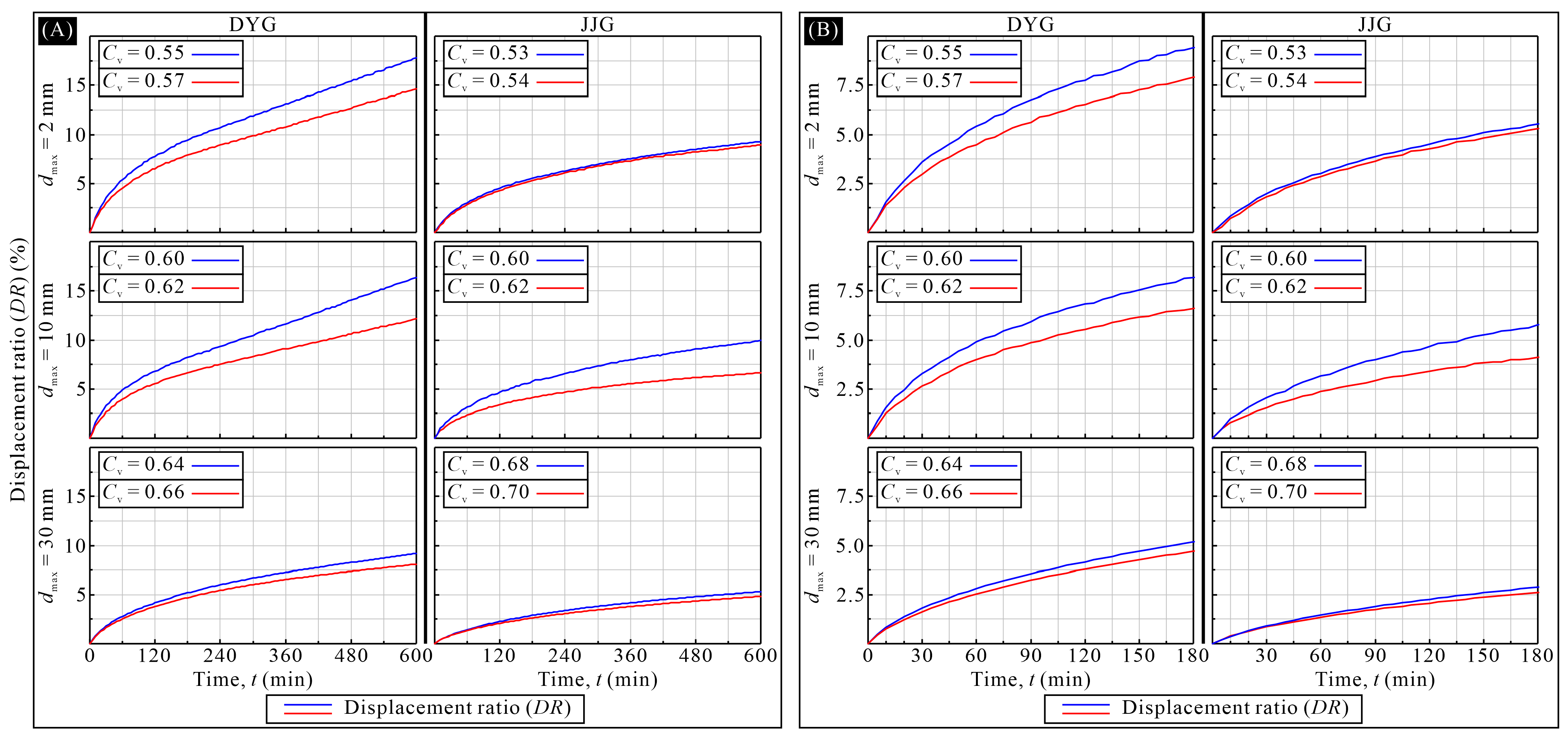
5.2. Response of the Water in Experimental Slurries to Hydraulic Forcing

In the displacement experiments on all 12 slurries (Table 1), only colorless clean water was collected, that is, the displacing fluid (Rhodamine B solution) did not flow through the tested slurries (Figure 3). Figure 6 and Figure 7 show the cumulative percentages of the displaced and displacing fluids (P_e and P_d) and the displacement ratio (DR) versus time graphs, respectively.

Twelve pairs of time series of P_e and P_d from six pairs of slurries of the same debris source and d_max and different C_v showed a similar pattern (Figure 6). For each of the 24 curves, a gentle to very gentle rising stage (from approximately t = 120 to 600 min) was preceded by a slightly steep rising one (from approximately t = 0 to 120 min). Six pairs of slurries of the three clastic materials (DYG-10, DYG-30, and JJG-10) exhibited an inverse relationship between P_e and P_d and C_v (Table 1 and Figure 6b,c,b′). The measurements of P_e and P_d were inversely proportional to d_max for slurries from the same debris source, although these slurries did not strictly compare in terms of C_v with each other. The P_e and P_d values measured at a given time in the DYG slurries were higher than those measured in the JJG slurries with the same d_max and similar C_v. P_e values for a given slurry plot were slightly above the P_d curve, except for DYG-2-0.55 and DYG-2-0.57 (Table 1 and Figure 6a).

Overall, the amount of displaced water was very low, despite the prolonged experimental period of 600 min (Figure 6). P_e achieved at the end of the experiment ranged from approximately 6 to 25%, with an average of only 14%. Accordingly, the lower P_d values measured at t = 600 min were on the order of 6 to 24%.

More generally, DR, following the same trend as P_e for the 12 slurries measured at the end of the experiment, was approximately 5–18% (10% average) (Figure 6 and Figure 7A). The DR values achieved at t = 10 and 180 min, corresponding to the longest durations of real debris-flow surges and debris-flow events [91,92], varied between 0.4 and 1.6% and 3 and 9%, respectively (Figure 7B). Furthermore, according to the negative correlation between DR and d_max (Figure 7A), the DR values of real, coarse-grained debris-flow slurries at t = 10 and 180 min should be lower than 1 and 5% (considering DYG-30-0.64, which had a higher DR than JJG-30), respectively (Figure 7B).

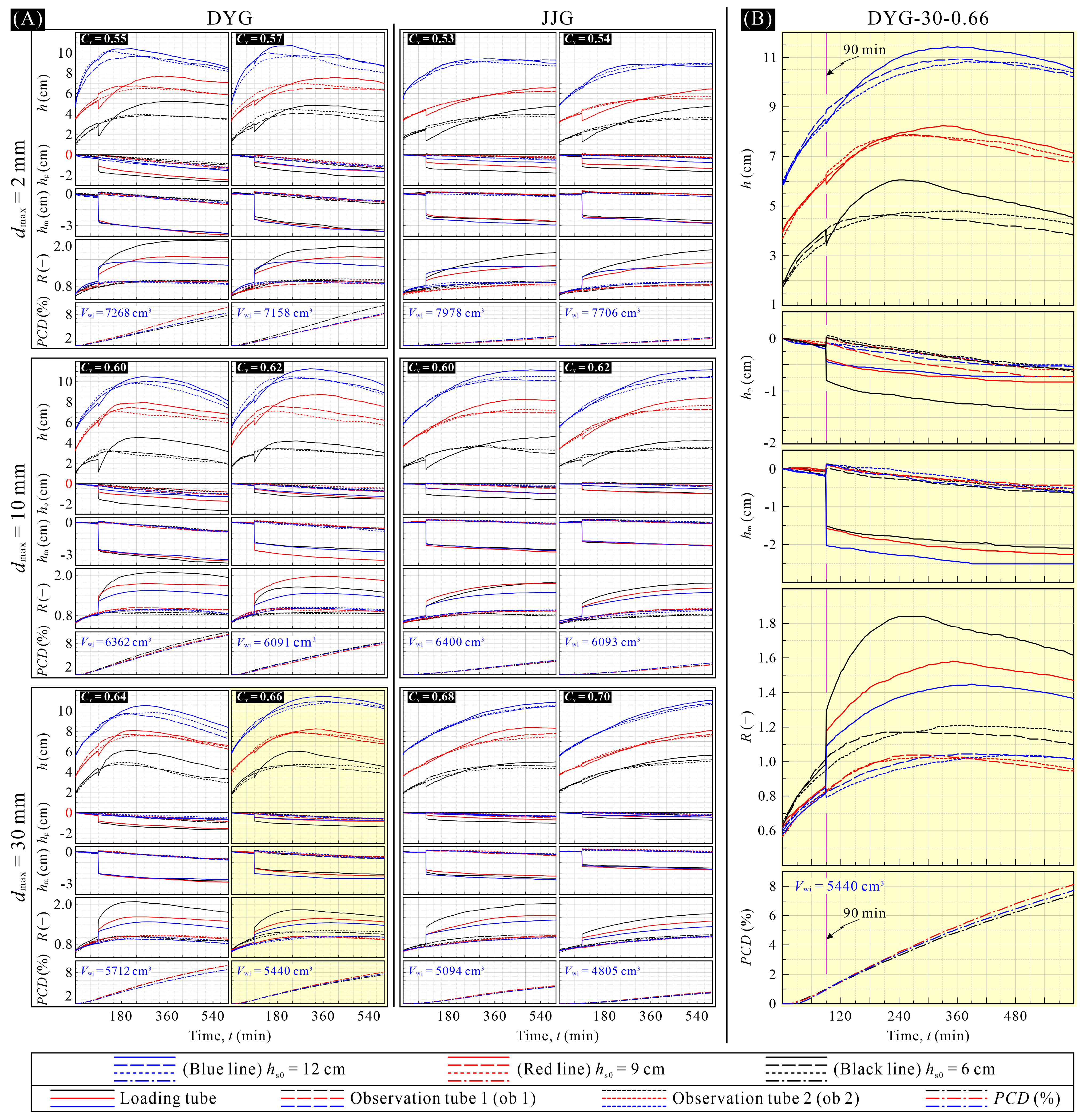
5.3. Response of the Water in Experimental Slurries to Mechanical Forcing

The test results of the relative motion experiment of the fluid (water) and solids under load in the 12 slurries listed in Table 1 are presented as a function of time in Figure 8A. Figure 8B shows an enlargement of the trends of the five variables (h, h_p, h_m, R in Figure 4, and PCD) monitored in DYG-30-0.66 (Table 1 and Figure 8A) with time.

There were multi-rank similarities between the test results of the DYG and JJG slurries, between the slurries from the same debris source but different d_max, between the slurries of the same detrital material but different C_v, and between three runs (with different h_s0, Figure 4) of the same slurry (Figure 8A). Specifically, each of the 13 curves for the 5 variables displays a similar pattern in all 36 test runs (Figure 8A), indicating that the results were reproducible. For simplicity, the results on all of the slurries are described below.

5.3.1. Initial Stage Before Loading (0–90 min)

Before loading at t = 90 min after the beginning of the test, all of the three piezometers exhibited a gradual rise in h of 0.6–4.7 cm, with an average of 1.9 cm. No discernible changes in h_p and h_m (<0.4 cm), in contrast with h, were observed. Consequently, an increase in R occurred, ranging from 0.06 to 0.40. More significantly, the PCD achieved at the end of this stage was only 0.1–1.4%. In particular, only a few cubic centimeters (average cumulative discharge of 4.3 cm³, with a maximum of 17.3 cm³) of water escaped onto the slurry surfaces during the first 30 min of the stage, which matches the minimal subsidence of the slurry surfaces indicated by h_m.

5.3.2. The Moment When Load Is Applied (90 min)

When the external load was imposed at t = 90 min, a sharp fall in h occurred in the loading tube, with decreases up to 1.2 cm depending on h_s0. In contrast, the two observation tubes showed a comparatively small increase in h (only up to 0.4 cm), which tended to decrease with increasing h_s0.

Interestingly, analogous response behaviors occurred in the h_p of the piezometer tubes themselves, with the loading piezometer lowered by 0.1–1.3 cm, and the observation tubes slightly elevated by 0.3 cm.

As expected, the response of h_m to the loading was similar to the changes observed in h and h_p. The h_m values around the loading tubes dramatically decreased by 1.2–2.6 cm, and those around the observation tubes increased slightly, with heights of 0.1–0.4 cm.

Accordingly, the R values of the loading tubes abruptly increased from 0.69–1.03 at t = 89 min to 0.92–1.52, whereas those of the observation tubes decreased slightly, and the amplitudes of the changes were only 0.01–0.04.

Equally important, loading caused little variation in the rate of increase in PCD.

5.3.3. The Stage in Which the h of the Loading Tube Is Lower than That of the Observational Piezometers

In the subsequent period of 10–220 min (average of 90 min), the previously lowered h for the loading tube increased slowly to a level comparable to that of the observational piezometers. For the loading tubes with h_s0 of 6 cm, within the appreciably affected range of loading, the recovery of the head required 10–210 min (average 105 min). Quite surprisingly, the h of the observational piezometers continued to rise slowly, following their original trend before loading, or even at lower rates than before loading, almost as though the loading event did not occur.

During this stage, the h_p and h_m values of all three piezometers decreased at extremely low rates (average 0.9 mm/50 min and 0.8 mm/50 min, respectively). Consequently, the differences in the R values between the loading and observational tubes widened further to the order of 0.21–0.88, and were anti-correlated with h_s0.

It is noteworthy that no obvious change in the rate of increase in PCD was observed at this stage relative to that during the 30–89 min stage.

5.3.4. The Stage in Which the h for the Loading Tube Is Higher than That for the Observational Piezometers

Compared to the end of the previous stage, the h of the loading tube increased up to 1.7 cm above that of the observational tubes, which lasted 290–500 min until the end of the experimental runs, except for DYG-2-0.57 with a h_s0 of 12 cm, JJG-2-0.53 with a h_s0 of 12 cm, and JJG-2-0.54 with a h_s0 of 12 cm. In this stage, the rate at which the h values of all of the piezometers changed was very slow, with maximum rising and falling rates of 0.9 and 0.4 cm/h, respectively, so that their time trends were dome-shaped (mainly DYG slurries) or even semi-dome-shaped (mainly JJG slurries).

The slowly descending trends of h_p and h_m were still as discernible as in the previous stage, with subsidence rates of approximately 0.2–1.5 and 0.2–1.4 mm/h, respectively.

At the end of the experiment at t = 600 min, the R values for the loading and observational tubes remained in the order of 1.28–2.15 and 0.79–1.17, respectively, and the differences in R between them were maintained at 0.28–1.18.

As expected from the change in h_m of the piezometers, the final PCD of the 36 runs was only 1.9–11.0%.

Taken together, loading caused significant and persistent changes in h, h_p, h_m, and R values for the loading tube, but little or no response of h, h_p, h_m, and R in the observation tubes, and a rate of increase in PCD occurred.

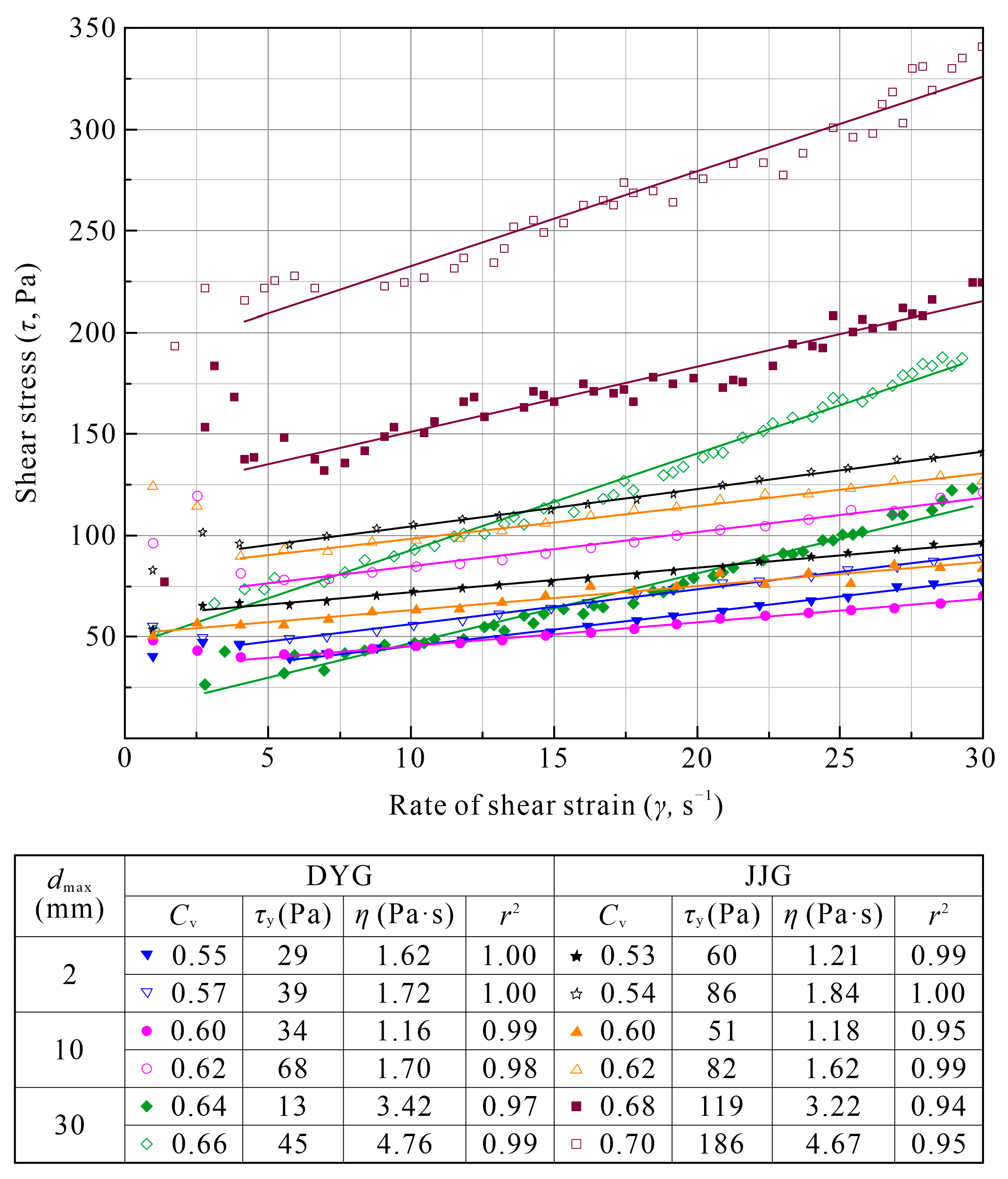
5.4. Rheology of Experimental Debris Flows

The results of the flow experiments on the 12 slurries (Table 1) are shown in Figure 9. The properties of the tested slurries (debris source, maximum grain diameter, d_max, and solid volume concentration, C_v), rheological parameters, including yield stress (τ_y) and viscosity (η) determined by using the Bingham model to fit the rheometrical data, and their r² are listed in the lower part of Figure 9.

The shear stress (τ) measured in all of the slurries was proportional to rate of shear strain (γ), showing that the slurries are Bingham fluid [1]. Twelve values of r² are in the order of 0.94–1.00 (mean = 0.98, with a standard deviation = 0.02), and quantitatively demonstrate that the rheometrical data can be fitted reasonably well by the Bingham model.

All six pairs of slurries of the same debris source and d_max exhibited an overall trend of increasing τ_y and η with C_v. This was consistent with the results of previous studies [10,54,88]. The magnitude of τ_y and η of the slurries of the sediments from different sites and of different d_max, of course, are not strictly comparable because of their extreme sensitivity to debris composition, grain-size distribution, and solid concentration [28].

6. Discussion

The results of the escape test of fluids, displacement experiment of water, relative motion experiment of water and solids, and rheometric test of slurries can be mutually verified, and they systematically support the theory that debris flows should be considered as single-phase flows.

6.1. Relative Motion of Fluid (Water) and Solids in Debris-Flow Bodies

Under both gravity and artificial hydraulic and mechanical forcing [76,93,94], no relative motion of water or fluid composed of water and fine-grained particles and solids (i.e., phase separation between fluid and solids [28]) occurs in both the experimental debris-flow bodies and static slurries. To be rigorous, water or fluid capable of moving independently of (coarser-grained) solids does not exist or is negligible. This demonstrates that water and solid particles of all sizes in debris flows move together as a single fluid. The sediments in such flows are deposited en masse by freezing [27,36,42,57,95], and the water drains mainly by evaporation.

The C_r values approaching 1 obtained in the escape test indicate the high mobility of the experimental debris flows and deposit geometry (Figure 5), similar to those of natural debris-flow deposits (depositional sheets or flat-topped lobes [20,26,96,97,98,99]).

The Solidity (S) values close to 1 of the experimental deposits quantitatively demonstrated the movement as a whole and the en masse deposition of water and solids in the experimental flows (Figure 5). The fact that no fluid or only a negligible quantity of water leaves the experimental deposits, despite the experiment being run on a tilting plane favorable for separation between fluid (if any) and solid phases (Figure 5), demonstrates in a straightforward manner that water (or fluid) independent of (coarser) solids is absent in debris flows. This is in agreement with some previous studies (Costa (1988) [2]; Figure 6c in Remaître et al. (2003) [100]; Figure 9 in Hürlimann et al. (2015) [54]; Figures 1b and 6 in D’Agostino et al. (2013) [8]).

The covariations of P_e and P_d with C_v and d_max observed in the displacement experiment are easily understood. The relatively higher P_e and P_d values measured in the DYG slurries compared to those in the JJG slurries of the same d_max and similar C_v should be associated with lower contents of fines (say < 0.0625 mm) of the DYG sediments (Figure 1). The small or even negligible discrepancies between P_e and P_d match the incompressibility of water and solids.

The dimensionless parameter DR enables the characterization of the relative motion of water and solids (if present). The low DR values of 5–18% achieved in this study, and in particular those estimated by considering the durations of real debris-flow surges and whole flow events and their d_max (<1 and 5%, respectively), show that even under artificial hydraulic forcing, water movement relative to solids in debris-flow bodies is very sluggish or even negligible. This strongly supports the conclusion reached from the escape test that the water and solids in debris flows move as a whole.

The experimental slurries before loading roughly corresponded to the scenarios of natural debris flows coming to rest. PCD of only 0.1–1.4% measured at t = 90 min, together with the results of the escape test and displacement experiment discussed above, show that both the lateral and vertical relative motions of water (fluid) and solids in debris-flow masses are extremely slow, especially with respect to the duration of debris flows.

The coupled measurements of h, h_p, h_m, and PCD (Figure 4 and Figure 8) enabled us to evaluate the response of the tested slurries and the water in them to loading, i.e., to artificial mechanical forcing.

The changes in h_m for the loading and observation tubes before and after loading indicate that loading causes plastic deformation of the slurries (i.e., flow of the slurries [1]). However, a close examination of the components of the loading-induced rise in h for the observation tubes (Δh) reveals that it is derived entirely from the uplift of the tubes (Δh_p) held up by the slurries, meaning that the contribution of the water movement under load to Δh is zero. In other words, the artificial mechanical forcing exerted around the loading tubes failed to drive the water toward the observation tubes, despite the proximity of the weight. This is consistent with the abrupt increase in R for the loading tubes and the stabilization of the rate of increase in PCD.

It takes up to 220 min for the “pressed” h in the loading tubes to rise back to the level comparable to that of the observational piezometers, which is also the cause for the extension of the difference in R between the two types of piezometers and stabilization of the rate of increase in PCD. This indicates that the movement of water in the slurries was greatly hindered.

Perhaps more importantly, the high R values (>1) for the loading tubes in all 36 relative-motion experimental runs were sustained for more than 510 min, and the durations of the R values (>0.7) for the 72 observation tubes in all 36 runs were also longer than 440 min, which far exceeded the durations of natural debris-flow events, especially the duration of individual debris-flow surges. Further, the higher h values for the loading tubes than the observational tubes (head difference), caused by loading, are maintained over a long period, ranging from 220 to >500 min, and the difference of between 0.20 and 1.23 (average 0.55, 108 data) in R between two types of piezometers, occurring after loading, lasts until the end of relative motion experiment (510 min). These results for R and h coincide with the low final PCD of only 1.9–11.0%, and further demonstrate that movement of water relative to solids can hardly occur in debris flows.

In summary, the results of the escape, displacement, and relative motion experiments immediately confirm that no relative motion of water (fluid) or solids occurs in debris flows, or is negligible. Water and solids in debris flows as a whole respond to applied stress, that is, they move at the same velocity and are deposited by freezing. Therefore, debris flows should be considered as single-phase flows.

6.2. Bulk Behavior of Debris Flows

The flow behavior of the experimental debris flows was fairly similar to that of Bingham materials (Figure 9), which shows that water and solids in debris flows move as a whole and that debris flows can be considered as a one-phase flow. This is because only continuous, homogeneous, isotropic, and monophasic (CHIMP) flows can exhibit Bingham behavior [7,11,101].

Hyperconcentrated (stream) flows are typical two-phase flows of water and sediment [4,9]. These flows, which often constitute the tail of debris-flow surges (Figure 13.6 in Pierson (1986) [43]), are more common than debris flows in mountain basins.

Here, we prepare a hyperconcentrated mixture of water and sediment using the DYG debris with a maximum grain diameter (d_max) of 30 mm investigated in this study (DYG-30; Figure 1). The solid volume concentration (C_v) of the mixture was 0.59, which is below the lower slurring limit (${\mathrm{C}}_{\mathrm{v}}^{\mathrm{h}}$) of 0.62. The mixture was tentatively tested rheologically using the large-scale rheometers described in Section 4.4, and the results obtained from the two trials are shown in Figure 10. For comparison, the flow curves of two experimental debris flows (DYG-30-0.64 and DYG-30-0.66; Table 1 and Figure 9) are depicted in this figure.

It can be seen from Figure 10 that the shear stress (τ) for the experimental hyperconcentrated flows, compared to those for the experimental debris flows, displays irregular, large amplitude fluctuations with the rate of shear strain (γ), which is in perfect agreement with those presented in Figure 3b,d in Yang et al. (2020) [53]. The values of r² achieved by fitting the data points for the two trials with the Bingham model are only 0.48 and 0.03. This indicates that there is no correlation between their τ and γ, i.e., that two-phase flows of water and sediment do not behave like Bingham fluids and cannot be described using the Bingham model. Various types of rheometers have been used extensively and successfully in debris-flow research [7,22,26,30,75,86,89]. Conversely, the use of rheometers to investigate the two-phase flows of sediment and water is problematic (the coupling connecting the variable-speed motor and impeller of the large rheometer described above is twisted off after only two trials) because of the rapid settlement of solids and subsequent phase segregation [10,73]. This strongly supports the theory that debris flows can be approximated as monophasic fluids.

Simultaneously, the comparisons shown in Figure 10 demonstrate more directly that the debris flows behave more like Bingham flows and are far from two-phase flows. In other words, debris flows should be treated as a single flow rather than as a two-phase flow.

Additionally, the flow processes occurring in mountainous areas, according to Pierson and Costa (1987) [1], can be reasonably classified as streamflow, hyperconcentrated flow, debris flow, and granular flow including debris avalanche (rock avalanche, sturzstrom, Pollet and Schneider (2004) [102]). The two-phase hypothesis of debris flows stems from biphasic hyperconcentrated flows, even saturated granular flows, being mistakenly (at least improperly) regarded as debris flows or even used to represent debris flows.

6.3. Transported Objects by Debris Flows

In light of the above discussion, debris flows are the flows of the fluids composed of water and sediment, similar to Bingham fluids. Clasts (solids) of any size in the continuous grain-size spectrum of the sediment comprising a debris flow, up to large boulders, are components of the flow (i.e., the fluid).

Debris-flow sediments are characteristically very poorly to extremely poorly sorted [9,103,104], i.e., well graded [12,21,96], which means that everything in debris flows is acting as the “fluid” [27]. In other words, the coarsest grains in debris flows (whose diameters are expressed here by D_max) can be as large as tens of centimeters, or even meter-sized, as long as no significant size discontinuities occur between them and other granular components finer than them [77].

Occurring as a fluid, one-phase debris flows can propagate alone and also function as a transporting medium by carrying larger clasts of >>D_max. These unusually large (outsized) clasts (boulders or blocks [20,69,105]) are objects transported by debris flows rather than components of the flows (Figure 1 in Rodine and Johnson (1976) [77]; Photo 1 in Li et al. (1983) [59]; Figure 8.17 in Johnson and Rodine (1984) [20]; Figure 10 in Jakob et al. (2000) [106]; Figure 11).

As discussed above, the results of the investigations of the relative motion of fluid (water) and solids and bulk behavior suggest that debris flows are much more similar to continuous, homogeneous, isotropic, and monophasic (CHIMP) flows than two-phase hyperconcentrated flows.

It is well known that rock masses are largely discontinuous, anisotropic, inhomogeneous, and non-elastic [36,42,107,108,109], but may be considered to be continuous, homogeneous, isotropic, and linearly elastic [110,111], which greatly simplifies complex rock mass behavior. In contrast, real debris flows themselves are close to CHIMP, and the two-phase hypothesis (approach) largely complicates debris flow problems. Most importantly, this could lead to confusion between peculiar (fascinating or surprising) debris-flow phenomena [4,20,112] and the relatively more common hyperconcentrated flow processes in mountain catchments. This directly affects the understanding, identification, assessment, and design of mitigation measures of debris flows.

7. Conclusions

The number of phases is a key consideration in the field of debris flow research and remains a matter of debate. Here, we experimentally investigated the number of phases in fully developed debris flows (i.e., the main bodies of debris flows) using six sediments with three maximum diameters of up to 30 mm from representative sandy and muddy debris-flow deposits in China. Fluid escape tests, displacement experiments, relative motion experiments, and rheometric tests were conducted using 12 slurries prepared with the sediments (two solid volume concentrations for each sediment). The results from the four types of experiments show that debris flows are close to one flow and far from two-phase flow.

Under both gravity and artificial hydraulic and mechanical forcing, no relative motion of water or fluid composed of water and fine-grained particles and solids (phase separation) occurred in both the experimental debris flows and static slurries. Water or fluid capable of moving independently of (coarser-grained) solids does not exist or is negligible. This demonstrates that water and solid particles of all sizes in debris flows move together as a single fluid and are deposited en masse via freezing.

The behavior of the experimental debris flows is fairly similar to that of Bingham materials, which is quite different from that of two-phase experimental hyperconcentrated flows. This shows that water and solids in debris flows move as a whole and that debris flows may be regarded as one-phase flow, considering that Bingham behavior is exhibited only by continuous, homogeneous, isotropic, and monophasic flows.

In conclusion, debris flows behave more like Bingham flows, are far from biphasic flow, and should be treated as one-phase flow rather than two-phase flow. The two-phase hypothesis seems to arbitrarily complicate debris-flow problems and, in practice, leads to confusion between peculiar debris-flow phenomena and common hyperconcentrated flow processes in mountain basins.

Clasts (solids) of any size, including those of meters, in the continuous grain-size spectrum of the sediment comprising a debris flow are the components of the flow. Monophasic debris flows can propagate alone and function as transporting medium by carrying blocks that are much coarser than the coarse end-member of their continuous gradation (transported object).

References

1. Pierson, T.C.; Costa, J.E. A rheologic classification of subaerial sediment-water flows. In Debris Flows/Avalanches: Process, Recognition and Mitigation; Costa, J.E., Wieczorek, G.F., Eds.; Geological Society of America Reviews in Engineering Geology: Boulder, CO, USA, 1987; pp. 1–12. [Google Scholar] [CrossRef]
2. Costa, J.E. Rheologic, geomorphic, and sedimentologic differentiation of water floods, hyperconcentrated flows, and debris flow. In Flood Geomorphology; Baker, V.R., Kochel, R.C., Patton, P.C., Eds.; John Wiley & Sons: New York, NY, USA, 1988; pp. 113–122. [Google Scholar]
3. Scott, K.M.; Wang, Y.Y. Debris Flows-Geologic Process and Hazard, Illustrated by a Surge Sequence at Jiangjia Ravine, Yunnan, China; Professional Paper 1671; U.S. Geological Survey: Reston, VA, USA, 2004. Available online: https://pubs.usgs.gov/pp/1671/ (accessed on 1 January 2024).
4. Coussot, P.; Meunier, M. Recognition, classification and mechanical description of debris flows. Earth-Sci. Rev. 1996, 40, 209–227. [Google Scholar] [CrossRef]
5. Coussot, P.; Ancey, C. Rheophysical classification of concentrated suspensions and granular pastes. Phys. Rev. E 1999, 59, 4445–4457. [Google Scholar] [CrossRef]
6. Davies, T.R.H. Debris-flow surges—Experimental simulation. J. Hydrol. 1990, 29, 18–46. Available online: https://www.jstor.org/stable/43944650 (accessed on 1 January 2024).
7. Sosio, R.; Crosta, G.B.; Frattini, P. Field observations, rheological testing and numerical modelling of a debris-flow event. Earth Surf. Process. Landf. 2007, 32, 290–306. [Google Scholar] [CrossRef]
8. D’Agostino, V.; Bettella, F.; Cesca, M. Basal shear stress of debris flow in the runout phase. Geomorphology 2013, 201, 272–280. [Google Scholar] [CrossRef]
9. Pierson, T.C. Hyperconcentrated flow-transitional process between water flow and debris flow. In Debris-Flow Hazards and Related Phenomena; Jakob, M., Hungr, O., Eds.; Praxis; Springer: Berlin/Heidelberg, Germany, 2005; pp. 159–202. [Google Scholar] [CrossRef]
10. Kaitna, R.; Rickenmann, D.; Schatzmann, M. Experimental study on the rheologic behaviour of debris flow material. Acta Geotech. 2007, 2, 71–85. [Google Scholar] [CrossRef]
11. Castelli, F.; Freni, G.; Lentini, V.; Fichera, A. Modelling of a debris flow event in the Enna area for hazard assessment. Procedia Eng. 2017, 175, 287–292. [Google Scholar] [CrossRef]
12. Hungr, O.; Morgan, G.C.; Kellerhals, R. Quantitative analysis of debris torrent hazards for design of remedial measures. Can. Geotech. J. 1984, 21, 663–677. [Google Scholar] [CrossRef]
13. Iverson, R.M. The physics of debris flows. Rev. Geophys. 1997, 35, 245–296. [Google Scholar] [CrossRef]
14. Iverson, R.M.; Logan, M.; Lahusen, R.G.; Berti, M. The perfect debris flow? Aggregated results from 28 large-scale experiments. J. Geophys. Res. Earth Surf. 2010, 115, 1–29. [Google Scholar] [CrossRef]
15. Kattel, P.; Kafle, J.; Fischer, J.T.; Mergili, M.; Tuladhar, B.M.; Pudasaini, S.P. Interaction of two-phase debris flow with obstacles. Eng. Geol. 2018, 242, 197–217. [Google Scholar] [CrossRef]
16. Brufau, P.; Garcia-Navarro, P.; Ghilardi, P.; Natale, L.; Savi, F. 1D mathematical modelling of debris flow. J. Hydraul. Res. 2000, 38, 435–446. [Google Scholar] [CrossRef]
17. Armanini, A.; Fraccarollo, L.; Rosatti, G. Two-dimensional simulation of debris flows in erodible channels. Comput. Geosci. 2009, 35, 993–1006. [Google Scholar] [CrossRef]
18. Rosatti, G.; Begnudelli, L. Two-dimensional simulation of debris flows over mobile bed: Enhancing the TRENT2D model by using a well-balanced Generalized Roe-type solver. Comput. Fluids 2013, 71, 179–195. [Google Scholar] [CrossRef]
19. Kowalski, J.; Mcelwaine, J.N. Shallow two-component gravity-driven flows with vertical variation. J. Fluid Mech. 2013, 714, 434–462. [Google Scholar] [CrossRef]
20. Johnson, A.M.; Rodine, J.R. Debris flow. In Slope Stability; Brunsden, D., Prior, D.B., Eds.; John Wiley & Sons: New York, NY, USA, 1984; pp. 257–361. [Google Scholar]
21. U.S. Department of Agriculture (USDA)-Natural Resources Conservation Service (NRCS), National Engineering Handbook, Chapter 3-Engineering Classification of Earth Materials; United States Department of Agriculture: Washington, DC, USA, 2012.
22. Major, J.J.; Pierson, T.C. Debris flow rheology: Experimental analysis of fine-grained slurries. Water Resour. Res. 1992, 28, 841–857. [Google Scholar] [CrossRef]
23. Pudasaini, S.P. A general two-phase debris flow model. J. Geophys. Res. Earth Surf. 2012, 117, F03010. [Google Scholar] [CrossRef]
24. Kaitna, R.; Palucis, M.C.; Yohannes, B.; Hill, K.M.; Dietrich, W.E. Effects of coarse grain size distribution and fine particle content on pore fluid pressure and shear behavior in experimental debris flows. J. Geophys. Res. Earth Surf. 2016, 121, 415–441. [Google Scholar] [CrossRef]
25. Kaitna, R.; Rickenmann, D. Flow of different material mixtures in a rotating drum. In Proceedings of the 4th International Conference on Debris-flow Hazard Mitigation: Mechanics, Prediction, and Assessment, Chengdu, China, 10–13 September 2007; Chen, C.L., Major, J.J., Eds.; Millpress: Rotterdam, The Netherlands, 2007; pp. 269–279. [Google Scholar]
26. Malet, J.-P.; Remaître, A.; Maquaire, O.; Ancey, C.; Locat, J. Flow susceptibility of heterogeneous marly formations. Implications for torrent hazard control in the Barcelonnette basin (Alpes-de-Haute-Provence, France). In Proceedings of the 3rd International Conference on Debris-Flow Hazard Mitigation: Mechanics, Prediction, and Assessment, Davos, Switzerland, 10–12 September 2003; Rickenmann, D., Chen, C.L., Eds.; Millpress: Rotterdam, The Netherlands, 2003; pp. 351–362. [Google Scholar]
27. Pierson, T.C. Dominant particle support mechanisms in debris flows at Mt Thomas, New Zealand, and implications for flow mobility. Sedimentology 1981, 28, 49–60. [Google Scholar] [CrossRef]
28. Phillips, C.J.; Davies, T.R.H. Determining rheological parameters of debris flow material. Geomorphology 1991, 4, 101–110. [Google Scholar] [CrossRef]
29. Marchi, L.; Arattano, M.; Deganutti, A.M. Ten years of debris-flow monitoring in the Moscardo Torrent (Italian Alps). Geomorphology 2002, 46, 1–17. [Google Scholar] [CrossRef]
30. Bardou, E.; Boivin, P.; Pfeifer, H.R. Properties of debris flow deposits and source materials compared: Implications for debris flow characterization. Sedimentology 2007, 54, 469–480. [Google Scholar] [CrossRef]
31. Sharp, R.P.; Nobles, L.H. Mudflow of 1941 at Wrightwood, southern California. Bull. Geol. Soc. Am. 1953, 64, 547–560. [Google Scholar] [CrossRef]
32. Costa, J.E.; Jarrett, R.D. Debris flows in small mountain stream channels of Colorado and their hydrologic implications. Environ. Eng. Geosci. 1981, 18, 309–322. [Google Scholar] [CrossRef]
33. Moscariello, A.; Marchi, L.; Maraga, F.; Mortara, G. Alluvial Fans in the Italian Alps: Sedimentary Facies and Processes. In Flood and Megaflood Processes and Deposits; Martini, I.P., Baker, V.R., Garzón, G., Eds.; Blackwell Publishing Ltd.: Oxford, UK, 2002; pp. 141–166. [Google Scholar] [CrossRef]
34. Berti, M.; Simoni, A. Prediction of debris flow inundation areas using empirical mobility relationships. Geomorphology 2007, 90, 144–161. [Google Scholar] [CrossRef]
35. Jakob, M. A size classification for debris flows. Eng. Geol. 2005, 79, 151–161. [Google Scholar] [CrossRef]
36. Eger, P.M.; Cagliari, J.; Aquino, C.D.; Coelho, O.G.W. Rheologic survey of mass transport events from the geologic record of an Andean Precordilleran slope. Geomorphology 2018, 315, 57–67. [Google Scholar] [CrossRef]
37. Hürlimann, M.; Coviello, V.; Bel, C.; Guo, X.; Berti, M.; Graf, C.; Hübl, J.; Miyata, S.; Smith, J.B.; Yin, H.Y. Debris-flow monitoring and warning: Review and examples. Earth-Sci. Rev. 2019, 199, 102981. [Google Scholar] [CrossRef]
38. Mckay, L.D.; Driese, S.G.; Smith, K.H.; Vepraskas, M.J. Hydrogeology and pedology of saprolite formed from sedimentary rock, eastern Tennessee, USA. Geoderma 2005, 126, 27–45. [Google Scholar] [CrossRef]
39. D’Agostino, V.; Cesca, M.; Marchi, L. Field and laboratory investigations of runout distances of debris flows in the Dolomites (Eastern Italian Alps). Geomorphology 2010, 115, 294–304. [Google Scholar] [CrossRef]
40. Remaître, A.; Malet, J.-P.; Maquaire, O. Geomorphology and kinematics of debris flows with high entrainment rates: A case study in the South French Alps. Comptes Rendus Geosci. 2011, 343, 777–794. [Google Scholar] [CrossRef]
41. Ilinca, V. Using morphometrics to distinguish between debris flow, debris flood and flood (Southern Carpathians, Romania). Catena 2021, 197, 104982. [Google Scholar] [CrossRef]
42. Carter, R.M. A discussion and classification of subaqueous mass-transport with particular application to grain-flow, slurry-flow, and fluxoturbidites. Earth-Sci. Rev. 1975, 11, 145–177. [Google Scholar] [CrossRef]
43. Pierson, T.C. Flow behavior of channelized debris flows, Mount St. Helens, Washington. In Hillslope Processes; Abrahms, A.D., Ed.; Routledge: London, UK, 1986; pp. 269–296. [Google Scholar]
44. Pérez, F.L. Matrix granulometry of catastrophic debris flows (December 1999) in central coastal Venezuela. Catena 2001, 45, 163–183. [Google Scholar] [CrossRef]
45. Ye, Z.M.; Xu, Z.M.; Li, B.; Su, X.; Shi, G.E.; Meng, J.K.; Tian, L. Generation and origin of persistent high excess pore water pressure in debris flows. Geomorphology 2024, 444, 108954. [Google Scholar] [CrossRef]
46. Li, J.C. Neotectonic feature of the Nujiang fault zone in western Yunnan. Seismol. Geol. 1998, 20, 312–320. (In Chinese) [Google Scholar]
47. Chang, C.W.; Lin, P.S.; Tsai, C.L. Estimation of sediment volume of debris flow caused by extreme rainfall in Taiwan. Eng. Geol. 2011, 123, 83–90. [Google Scholar] [CrossRef]
48. Klubertanz, G.; Laloui, L.; Vulliet, L. Identification of mechanisms for landslide type initiation of debris flows. Eng. Geol. 2009, 109, 114–123. [Google Scholar] [CrossRef]
49. Zhou, Z.H.; Ren, Z.; Wang, K.; Yang, K.; Tang, Y.J.; Tian, L.; Xu, Z.M. Effect of excess pore pressure on the long runout of debris flows over low gradient channels: A case study of the Dongyuege debris flow in Nu River, China. Geomorphology 2018, 308, 40–53. [Google Scholar] [CrossRef]
50. Tang, Y.J.; Xu, Z.M.; Shao, Z.C.; Ren, Z.; Wang, K.; Yang, K.; Tian, L. Laboratory investigations of the role of biofilms on stream-bed surfaces in debris-flow runout. Earth Surf. Process. Landf. 2020, 45, 999–1012. [Google Scholar] [CrossRef]
51. Tang, Y.J.; Xu, Z.M.; Yang, T.Q.; Zhou, Z.H.; Wang, K.; Ren, Z.; Yang, K.; Tian, L. Impacts of small woody debris on slurrying, persistence, and propagation in a low-gradient channel of the Dongyuege debris flow in Nu River, Southwest China. Landslides 2018, 15, 2279–2293. [Google Scholar] [CrossRef]
52. Yang, K.; Xu, Z.M.; Ren, Z.; Wang, K.; Tang, Y.J.; Tian, L.; Luo, J.Y.; Gao, H.Y. Physico-mechanical performance of debris-flow deposits with particular reference to characterization and recognition of debris flow-related sediments. J. Cent. South Univ. 2020, 27, 2726–2744. [Google Scholar] [CrossRef]
53. Yang, K.; Xu, Z.M.; Tian, L.; Wang, K.; Ren, Z.; Tang, Y.J.; Luo, J.Y.; Gao, H.Y. Significance of coarse clasts in viscous debris flows. Eng. Geol. 2020, 272, 105665. [Google Scholar] [CrossRef]
54. Hürlimann, M.; Mcardell, B.W.; Rickli, C. Field and laboratory analysis of the runout characteristics of hillslope debris flows in Switzerland. Geomorphology 2015, 232, 20–32. [Google Scholar] [CrossRef]
55. Das, B.M. Advanced Soil Mechanics, 3rd ed.; Taylor & Frances: New York, NY, USA, 2008. [Google Scholar]
56. Crosta, G.B.; Cucchiaro, S.; Frattini, P. Validation of semi-empirical relationships for the definition of debris-flow behavior in granular materials. In Proceedings of the 3rd International Conference on Debris-Flow Hazard Mitigation: Mechanics, Prediction, and Assessment, Davos, Switzerland, 10–12 September 2003; Rickenmann, D., Chen, C.L., Eds.; Millpress: Rotterdam, The Netherlands, 2003; pp. 821–831. [Google Scholar]
57. Godt, J.W.; Coe, J.A. Alpine debris flows triggered by a 28 July 1999 thunderstorm in the central Front Range, Colorado. Geomorphology 2007, 84, 80–97. [Google Scholar] [CrossRef]
58. Kim, Y.; Nakagawa, H.; Kawaike, K.; Zhang, H. Study on hydraulic characteristics of sabo dam with a flap structure for debris flow. Int. J. Sediment Res. 2017, 32, 452–464. [Google Scholar] [CrossRef]
59. Li, J.; Yuan, J.M.; Bi, C.; Luo, D.F. The main features of the mudflow in Jiangjia Ravine. Z. Für Geomorphol. 1983, 27, 325–341. [Google Scholar] [CrossRef]
60. Zhang, S.C. A comprehensive approach to the observation and prevention of debris flows in China. Nat. Hazards 1993, 7, 1–23. [Google Scholar] [CrossRef]
61. Chen, J.; He, Y.P.; Wei, F.Q. Debris flow erosion and deposition in Jiangjia Gully, Yunnan, China. Environ. Geol. 2005, 48, 771–777. [Google Scholar] [CrossRef]
62. Kang, Z.C.; Cui, P.; Wei, F.Q.; He, S.F. Data Collection of Dongchuan Debris Flow Observation and Research Station Chinese Academy of Sciences (1961–1984); Science Press: Beijing, China, 2006. (In Chinese) [Google Scholar]
63. Kang, Z.C.; Cui, P.; Wei, F.Q.; He, S.F. Data Collection of Dongchuan Debris Flow Observation and Research Station Chinese Academy of Sciences (1995–2000); Science Press: Beijing, China, 2007. (In Chinese) [Google Scholar]
64. Yang, H.J.; Wei, F.Q.; Hu, K.H.; Wang, C.C. Determination of the suspension competence of debris flows based on particle size analysis. Int. J. Sediment Res. 2014, 29, 73–81. [Google Scholar] [CrossRef]
65. Yu, B.; Zhu, Y.; Wang, T.; Zhu, Y.B. A 10-min rainfall prediction model for debris flows triggered by a runoff induced mechanism. Environ. Earth Sci. 2016, 75, 216. [Google Scholar] [CrossRef]
66. Guo, X.J.; Li, Y.; Cui, P.; Yan, H.; Zhuang, J.Q. Intermittent viscous debris flow formation in Jiangjia Gully from the perspectives of hydrological processes and material supply. J. Hydrol. 2020, 589, 125184. [Google Scholar] [CrossRef]
67. Yang, H.J.; Zhang, S.J.; Hu, K.H.; Wei, F.Q.; Wang, K.; Liu, S. Field observation of debris-flow activities in the initiation area of the Jiangjia Gully, Yunnan Province, China. J. Mt. Sci. 2022, 19, 1602–1617. [Google Scholar] [CrossRef]
68. Zhao, T.; Zhou, G.G.D.; Sun, Q.C.; Crosta, G.B.; Song, D.R. Slope erosion induced by surges of debris flow: Insights from field experiments. Landslides 2022, 19, 2367–2377. [Google Scholar] [CrossRef]
69. Wagreich, M.; Strauss, P.E. Source area and tectonic control on alluvial-fan development in the Miocene Fohnsdorf intramontane basin, Austria. In Alluvial Fans: Geomorphology, Sedimentology, Dynamics; Harvey, A.M., Mather, A.E., Stokes, M., Eds.; Geological Society, London, Special Publications: London, UK, 2005; Volume 251, pp. 207–216. [Google Scholar] [CrossRef]
70. Legg, N.T.; Meigs, A.J.; Grant, G.E.; Kennard, P. Debris flow initiation in proglacial gullies on Mount Rainier, Washington. Geomorphology 2014, 226, 249–260. [Google Scholar] [CrossRef]
71. Martin, Y.E.; Johnson, E.A.; Chaikina, O. Gully recharge rates and debris flows: A combined numerical modeling and field-based investigation, Haida Gwaii, British Columbia. Geomorphology 2017, 278, 252–268. [Google Scholar] [CrossRef]
72. GB/T 50123–2019; Standard for Geotechnical Testing Method. Ministry of Housing and Urban-Rural Development of the P.R. China & State Administration for Market Regulation: Beijing, China, 2019. (In Chinese)
73. Scotto Di Santolo, A.; Pellegrino, A.M.; Evangelista, A.; Coussot, P. Rheological behaviour of reconstituted pyroclastic debris flow. Géotechnique 2012, 62, 19–27. [Google Scholar] [CrossRef]
74. Tattersall, G.H. The rationale of a two-point workability test. Mag. Concr. Res. 1973, 25, 169–172. [Google Scholar] [CrossRef]
75. Schatzmann, M.; Bezzola, G.R.; Minor, H.-E.; Windhab, E.J.; Fischer, P. Rheometry for large-particulated fluids: Analysis of the ball measuring system and comparison to debris flow rheometry. Rheol. Acta 2009, 48, 715–733. [Google Scholar] [CrossRef]
76. De Haas, T.; Braat, L.; Leuven, J.R.F.W.; Lokhorst, I.R.; Kleinhans, M.G. Effects of debris flow composition on runout, depositional mechanisms, and deposit morphology in laboratory experiments. J. Geophys. Res. Earth Surf. 2015, 120, 1949–1972. [Google Scholar] [CrossRef]
77. Rodine, J.D.; Johnson, A.M. The ability of debris, heavily freighted with coarse clastic materials, to flow on gentle slopes. Sedimentology 1976, 23, 213–234. [Google Scholar] [CrossRef]
78. Simoni, A.; Mammoliti, M.; Berti, M. Uncertainty of debris flow mobility relationships and its influence on the prediction of inundated areas. Geomorphology 2011, 132, 249–259. [Google Scholar] [CrossRef]
79. Stancanelli, L.M.; Rosatti, G.; Begnudelli, L.; Armanini, A.; Foti, E. Single or Two-Phase Modelling of Debris-Flow? A Systematic Comparison of the Two Approaches Applied to a Real Debris Flow in Giampilieri Village (Italy). In Landslide Science and Practice; Margottini, C., Canuti, P., Sassa, K., Eds.; Springer: Berlin/Heidelberg, Germany, 2013; pp. 277–283. [Google Scholar] [CrossRef]
80. Baselt, I.; De Oliveira, G.Q.; Fischer, J.-T.; Pudasaini, S.P. Deposition morphology in large-scale laboratory stony debris flows. Geomorphology 2022, 396, 107992. [Google Scholar] [CrossRef]
81. Willhite, G.P. Waterflooding; Society of Petroleum Engineers: Richardson, TX, USA, 1986. [Google Scholar] [CrossRef]
82. Bear, J. Dynamics of Fluids in Porous Media; Dover: New York, NY, USA, 1988. [Google Scholar]
83. ASTM D 2434–68; Standard Test Method for Permeability of Granular Soils (Constant Head). ASTM International: West Conshohocken, PA, USA, 2006.
84. Eckersley, J.D. Instrumented laboratory flowslides. Géotechnique 1990, 40, 489–502. [Google Scholar] [CrossRef]
85. Fanchi, J.R. Chapter 6-Fluid Properties. Shared Earth Modeling; Butterworth-Heinemann: Amsterdam, The Netherlands, 2002; pp. 87–107. [Google Scholar] [CrossRef]
86. Coussot, P.; Piau, J.M. On the behavior of fine mud suspensions. Rheol. Acta 1994, 33, 175–184. [Google Scholar] [CrossRef]
87. Coussot, P.; Nguyen, Q.D.; Huynh, H.T.; Bonn, D. Avalanche Behavior in Yield Stress Fluids. Phys. Rev. Lett. 2002, 88, 175501. [Google Scholar] [CrossRef]
88. Kameda, J.; Morisaki, T. Sensitivity of clay suspension rheological properties to pH, temperature, salinity, and smectite-quartz ratio. Geophys. Res. Lett. 2017, 44, 9615–9621. [Google Scholar] [CrossRef]
89. O’brien, J.S.; Julien, P.Y. Laboratory analysis of mudflow properties. J. Hydraul. Eng. 1988, 114, 877–887. [Google Scholar] [CrossRef]
90. Tattersall, G.H.; Bloomer, S.J. Further development of the two-point test for workability and extension of its range. Mag. Concr. Res. 1979, 31, 202–210. [Google Scholar] [CrossRef]
91. Major, J.J. Gravity-driven consolidation of granular slurries: Implications for debris-flow deposition and deposit characteristics. J. Sediment. Res. 2000, 70, 64–83. [Google Scholar] [CrossRef]
92. Chiarle, M.; Iannotti, S.; Mortara, G.; Deline, P. Recent debris flow occurrences associated with glaciers in the Alps. Glob. Planet. Change 2007, 56, 123–136. [Google Scholar] [CrossRef]
93. Collins, B.D.; Stock, G.M. Rockfall triggering by cyclic thermal stressing of exfoliation fractures. Nat. Geosci. 2016, 9, 395–400. [Google Scholar] [CrossRef]
94. D’Arcy, M.; Roda-Boluda, D.C.; Whittaker, A.C. Glacial-interglacial climate changes recorded by debris flow fan deposits, Owens Valley, California. Quat. Sci. Rev. 2017, 169, 288–311. [Google Scholar] [CrossRef]
95. Hampton, M.A. Competence of fine-grained debris flows. J. Sediment. Petrol. 1975, 45, 834–844. [Google Scholar] [CrossRef]
96. Pierson, T.C. Erosion and deposition by debris flows at Mt Thomas, North Canterbury, New Zealand. Earth Surf. Process. Landf. 1980, 5, 227–247. [Google Scholar] [CrossRef]
97. Innes, J.L. Debris flows. Prog. Phys. Geogr. 1983, 7, 469–501. [Google Scholar] [CrossRef]
98. Cruden, D.M.; Varnes, D.J. Landslide types and processes. In Landslides: Investigation and Mitigation; Turner, A.K., Schuster, R.L., Eds.; Transportation Research Board Spec. Rep.: Washington, DC, USA, 1996; Volume 247, pp. 36–75. [Google Scholar]
99. Palucis, M.C.; Ulizio, T.P.; Fuller, B.; Lamb, M.P. Flow resistance, sediment transport, and bedform development in a steep gravel-bedded river flume. Geomorphology 2018, 320, 111–126. [Google Scholar] [CrossRef]
100. Remaître, A.; Malet, J.-P.; Maquaire, O.; Ancey, C. Study of a debris-flow Study of a debris-flow event by coupling a geomorphological and a rheological investigation, example of the Faucon stream (Alpes-de-Haute-Provence, France). In Proceedings of the 3rd International Conference on Debris-Flow Hazard Mitigation: Mechanics, Prediction, and Assessment, Davos, Switzerland, 10–12 September 2003; Rickenmann, D., Chen, C.L., Eds.; Millpress: Rotterdam, The Netherlands, 2003; pp. 375–385. [Google Scholar]
101. Quan Luan, B.; Remaitre, A.; Van Asch, T.W.J.; Malet, J.-P.; Van Westen, C.J. Analysis of debris flow behavior with a one dimensional run-out model incorporating entrainment. Eng. Geol. 2012, 128, 63–75. [Google Scholar] [CrossRef]
102. Pollet, N.; Schneider, J.L.M. Dynamic disintegration processes accompanying transport of the Holocene Flims sturzstrom (Swiss Alps). Earth Planet. Sci. Lett. 2004, 221, 433–448. [Google Scholar] [CrossRef]
103. Crosta, G.B.; Frattini, P. Controls on modern alluvial fan processes in the central Alps, northern Italy. Earth Surf. Process. Landf. 2004, 29, 267–293. [Google Scholar] [CrossRef]
104. Jakob, M.; Friele, P. Frequency and magnitude of debris flows on Cheekye River, British Columbia. Geomorphology 2010, 114, 382–395. [Google Scholar] [CrossRef]
105. Mcardell, B.W.; Bartelt, P.; Kowalski, J. Field observations of basal forces and fluid pore pressure in a debris flow. Geophys. Res. Lett. 2007, 34, L07406. [Google Scholar] [CrossRef]
106. Jakob, M.; Anderson, D.; Fuller, T.; Hungr, O.; Ayotte, D. An unusually large debris flow at Hummingbird Creek, Mara Lake, British Columbia. Can. Geotech. J. 2000, 37, 1109–1125. [Google Scholar] [CrossRef]
107. Schramm, J.-M.; Weidinger, J.T.; Ibetsberger, H.J. Petrologic and structural controls on geomorphology of prehistoric Tsergo Ri slope failure, Langtang Himal, Nepal. Geomorphology 1998, 16, 107–121. [Google Scholar] [CrossRef]
108. Davies, T.R.H.; Mcsaveney, M.J.; Boulton, C.J. Elastic strain energy release from fragmenting grains: Effects on fault rupture. J. Struct. Geol. 2012, 38, 265–277. [Google Scholar] [CrossRef]
109. Brideau, M.A.; Yan, M.; Stead, D. The role of tectonic damage and brittle rock fracture in the development of large rock slope failures. Geomorphology 2009, 103, 30–49. [Google Scholar] [CrossRef]
110. Harrison, J.P.; Hudson, J.A. Engineering Rock Mechanics: Part 2 Illustrative Worked Examples; Pergamon: Rotterdam, The Netherlands, 2000. [Google Scholar]
111. Jing, L. A review of techniques, advances and outstanding issues in numerical modelling for rock mechanics and rock engineering. Int. J. Rock Mech. Min. Sci. 2003, 40, 283–353. [Google Scholar] [CrossRef]
112. Hampton, M.A. Buoyancy in debris flows. J. Sediment. Res. 1979, 49, 753–758. [Google Scholar] [CrossRef]
Figure 3. Schematic diagram of the set-up for the displacement experiment of fluid (water) in debris-flow slurries, showing the locations of the recharge container holding displacing fluid (red Rhodamine B solution), constant head, specimen cell containing slurry, collectors for the overflow and outflow, and electronic scales.
Applsci 15 04282 g003
Figure 4. Schematic diagram of the set-up of relative motion experiment of fluid (water) and solids showing the bucket containing the tested slurry, piezometers, weight serving as the applied surface load, and monitored variables (h, hp, hm, he, and hs).
Applsci 15 04282 g004
Figure 5. Orthophotos and scanned images (isopach maps) of experimental debris-flow deposits and a negligible amount of fluid (clear water) leaving five deposits, on a sloping (5°) surface. The size of the square grid providing scale is 10 cm × 10 cm. White dashed line circles on the photos indicate the initial positions of cylindrical containers holding slurry of two sizes of 10 and 30 cm in diameter. Maximum grain size (dmax), solid volume concentration (Cv), volume of tested slurries (V), surface area including convex sides (As) and inundated area (Ai) of deposits, coefficient of runout (Cr), Solidity (S), volume of the water contained in the tested slurries (Vwi), that escaping from deposits (Vwe), and % Vwe in Vwi are given in the lower part of the figure. “-“ represents no fluid leaving.
Applsci 15 04282 g005
Figure 6. Time trends of cumulative percentages of displaced and displacing fluids (Pe and Pd) in the initial amount of water (Vwi, cm3) contained in the 12 tested slurries of six clastic materials of three dmax from two sites of debris flows, the DYG (ac) and JJG (a′c′).
Applsci 15 04282 g006
Figure 7. Displacement ratio (DR) as a function of time for the 12 slurries (Table 1 and Figure 6). (A) for 0–600 min. (B) for 0–180 min.
Applsci 15 04282 g007
Figure 8. Changes in the monitoring data obtained in the relative motion experiment of water and solids in 12 slurries under load with time. These data include the hydraulic head (h), elevation of the piezometers (hp), and slurry surface of (hm) (negative values represent a drop in elevation) (Figure 4), relative excess water pressure (R), and percentage of cumulative discharge (PCD) of water in the initial amount of water in the tested slurry (Vwi, cm3). The locations of the loading tube, observation tubes 1 and 2, and hs0 (initial measured depths, 6, 9, and 12 cm) are shown in Figure 4. (A) Individual slurries given in Table 1. (B) Enlargement of time trends of five variables (h, hp, hm, R, and PCD) monitored at three initial depths in the DYG-30-0.66 slurry.
Applsci 15 04282 g008
Figure 9. Rheological data points, optimal straight-line fits, and rheological parameters, including yield stress (τy, Pa), viscosity (η, Pa·s) and their coefficients of determination (r2), for 12 experimental slurries (Table 1), showing a linear relationship between shear stress (τ) and rate of shear strain (γ), i.e., the similarity of the flow behavior of the slurry flows to the Bingham behavior.
Applsci 15 04282 g009
Figure 10. Flow curves for experimental hyperconcentrated mixture of Cv = 0.59 compared to those for two experimental debris-flow mixtures of Cv = 0.64, and 0.66, prepared with the same debris (DYG-30, with a lower slurring limit ( C v h ) of 0.62, Table 1 and Figure 9), showing that debris flows are close to one-phase Bingham flow, and far from two-phase hyperconcentrated flow. r2 is the coefficient of determination obtained by fitting rheological data using the Bingham model (dashed lines).
Applsci 15 04282 g010
Figure 11. The Dongyuege (DYG) debris-flow deposit and unusually large blocks transported by the flow, showing the constituent sediment of one-phase debris flows acting as transporting medium and outsized blocks serving as transported objects by the flows. (a,a′) A cross-section of the well-preserved remnant temporary dam (27°38′21.53″ N, 98°44′4.71″ E) 0.5 km upstream of the fan apex, which was excavated during the sampling campaign on 6–12 November 2019. An outsized boulder with a maximum dimension of approximately 2 m (object transported by the flow) is submerged in the debris-flow diamicton composed of clasts with diameters of approximately <50 cm (the debris-flow deposit). The view is toward the left bank of the DYG Creek. The man is for scale. Photo by Jun-Yao, Luo. (b,b′) The DYG alluvial fan, nine months after the occurrence of the catastrophic debris-flow event. A temporary road was constructed through the debris-flow deposit to look for the people buried by the deposit. The labeled outsized boulders with diameters of up to 9 m from the upstream channel are transported objects contrasted with debris-flow sediments acting as transporting medium. The view is toward the mouth of DYG Creek. The man on the road is for scale. Photo by Qing-Fei, Zhang.
Applsci 15 04282 g011