Ice Thickness Detection of Transmission Lines Based on Cross-Guide-UNet

Abstract

The presence of ice on transmission lines threatens their integrity. The thickness of ice is crucial with respect to the autonomous operation of de-icing robots. Therefore, we propose a Cross-Guide-UNet (CG-UNet) model for detecting the thickness of ice on ice-covered transmission lines. The CG-UNet model uses an encoder–decoder architecture and incorporates a cross-guide module (CGM) at the crosslayer connection of the model. Initially, we redesign the attention calculation method to suit the shape characteristics of transmission lines. Channel and spatial attention are computed for the encoder and decoder features, respectively. Subsequently, the attention weight is cross-applied to the encoder and decoder features, allowing for comprehensive utilization of feature information to guide the generation of ice-covered edges. Additionally, we introduce a joint loss function comprising cross-entropy loss and boundary loss for model training, enhancing the distinction of easily confused edge pixels. The CG-UNet model effectively detects ice-covered edges through experimental analysis, achieving optimal dataset scale (ODS) and optimal image scale (OIS) scores of 0.934 and 0.938, respectively. The thickness detection error is constrained within 7.2%. These results confirm that the proposed algorithm can provide a control basis for the high-precision operation of de-icing robots.

1. Introduction

Nowadays, electricity plays an important role in the daily routines of individuals, underlining the importance of a reliable power supply system. Overhead transmission lines serve as the primary conduit for electricity transmission, making the stability of these lines pivotal for the uninterrupted functioning of the power grid. However, owing to their elevated positioning, transmission lines are highly vulnerable to adverse weather conditions and environmental factors, including strong winds and thunderstorms, as well as the accumulation of ice and snow [1,2]. Ice buildup on transmission lines represents a common fault type that disrupts the operation and maintenance of power systems [3,4]. Severe ice cover can even cause transmission towers to collapse, disrupting people’s daily lives [5,6].

In order to effectively solve the problem of ice on transmission lines and ensure the stable operation of the power system, our team developed an intelligent de-icing robot, which is equipped with a camera module, vibration module, main control module, and AI module. This robot can accurately measure the ice layer thickness on iced transmission lines in real time and precisely calculate the vibration intensity required for efficient de-icing based on the thickness. Ice layers of different thicknesses have distinct characteristics and require significantly different vibration intensities. Thin ice layers are fragile, and excessive vibration intensity will waste energy and damage the lines, while thick ice layers need sufficient vibration to be removed. Our robot can dynamically adjust the vibration intensity to precisely adapt to various ice layers, minimizing the impact on the lines while de-icing and strongly ensuring the normal operation of the power system.

The detection of ice thickness on transmission lines primarily involves two approaches: mechanical modeling and image detection. Mechanical modeling entails calculating ice thickness by constructing a physical model [7]. Zhong et al. [8] achieved good results in artificial icing experiments by constructing a cylindrical array-based ice monitoring device and using a Makkonen model and related algorithms to measure ice weight and invert environmental parameters to detect ice thickness. Yang et al. [9] established a state equation for transmission lines and used an iterative method based on axial tension measurement to detect the equivalent ice thickness of 500 kV overhead lines. Their accuracy was verified through practical cases and finite element simulations. However, this method is susceptible to wind load interference and relies on specific line parameters for measurement accuracy, which limits its applicability in difficult parameter acquisition scenarios. However, this study has shortcomings in terms of adaptability to complex environments and measurement accuracy of some parameters. When calculating the thickness of ice layers through mechanical modeling, environmental factors are usually ignored [10]. This will cause a deviation between the actual ice and the model calculation results. For example, in low-temperature, high-humidity, and light-wind environments, micro vibrations of the circuit affect the condensation and growth of ice layers, and mechanical modeling does not consider these changes, which cannot provide accurate operational basis for de-icing robots. Image detection has emerged as a popular method, wherein images of ice-covered transmission lines are captured using image acquisition, devices and ice thickness is subsequently determined through image algorithms [11]. Image detection offers high safety and reliability compared with alternative methods [12]. At present, most detection methods use semantic segmentation technology, which divides the foreground and background through computer vision technology [13]. The Sharp U-Net [14] architecture was used to design deep convolution and spatial filters specifically for encoders to improve segmentation performance. Zunair et al. [15] conducted research on short-range context modeling and proposed an effective single-stage learning paradigm. Varshney et al. [16] employed a fully convolutional neural network for the semantic segmentation of ice cover images, subsequently using the segmented images to calculate ice thickness. Wang et al. [17] developed intelligent ice detection equipment and used the lightweight neural network MobileNetV3 for ice thickness detection. Nusantika et al. [18] introduced an enhanced multi-threshold algorithm to separate ice-covered pixels and employed morphological enhancement to identify regions of interest. Although these image detection methods use semantic segmentation algorithms to determine ice thickness and detect ice-covered edges, the high accuracy required by de-icing robots with respect to the determination of ice thickness necessitates a different approach. Hence, we used an edge detection algorithm to identify the upper and lower edges of ice-covered transmission lines and subsequently calculate the difference in ice thickness before and after ice coverage to accurately determine ice thickness.

Although image detection methods have the advantages of safety and reliability over mechanical modeling methods, existing methods for calculating ice thickness cannot meet the high-precision calculation needs of de-icing robots. When there are obstructions in the surrounding area, the semantic segmentation model is prone to misjudgment, missing the ice layer area and increasing the calculation error of ice thickness. In some practical situations, misjudgment can lead to excessive vibration of the de-icing robot on thin ice layers, damaging the circuit, and insufficient vibration on thick ice layers, resulting in a poor de-icing effect. Therefore, this article proposes a new edge detection algorithm to detect the upper and lower edges of ice-covered transmission lines and then calculate the thickness difference before and after icing to obtain accurate ice thickness. Due to the direct relationship between the thickness of detection and the intensity of vibration, the accuracy requirements for edge detection are more stringent. This study improved the neural network model and loss function to enable the model to more accurately predict the edges of ice-covered transmission lines. The CG-UNet edge detection algorithm proposed in this article adopts the framework of an encoder and a decoder. In response to the problem of insufficient feature fusion between encoding and decoding, a novel cross-guide module is proposed at the crosslayer connection between encoding and decoding. This innovative design significantly improves the guidance effect of the image upsampling restoration process. Secondly, in response to the problem of confusion in ice edge pixel detection, the loss function was improved by designing a joint loss function from both local and global perspectives, effectively enhancing the model’s ability to distinguish pixels near the edges. The main contributions of this study can be summarized as follows:

• Dataset innovation: We developed an edge detection dataset specifically designed for ice-covered transmission lines. This dataset provides rich samples for model training.
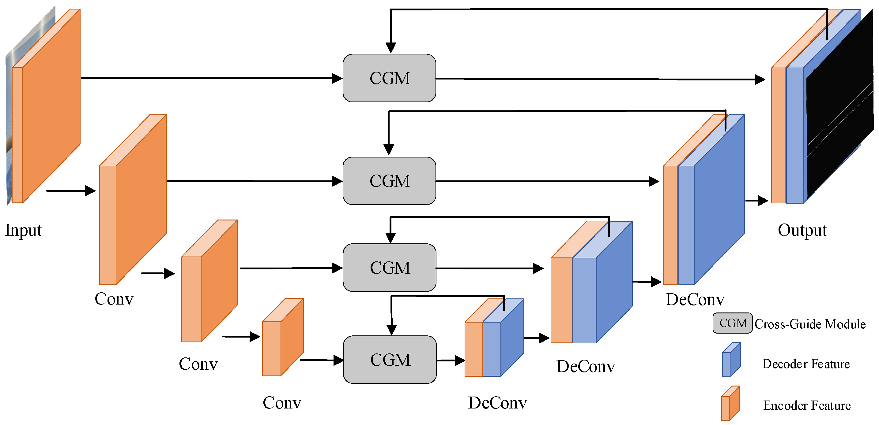
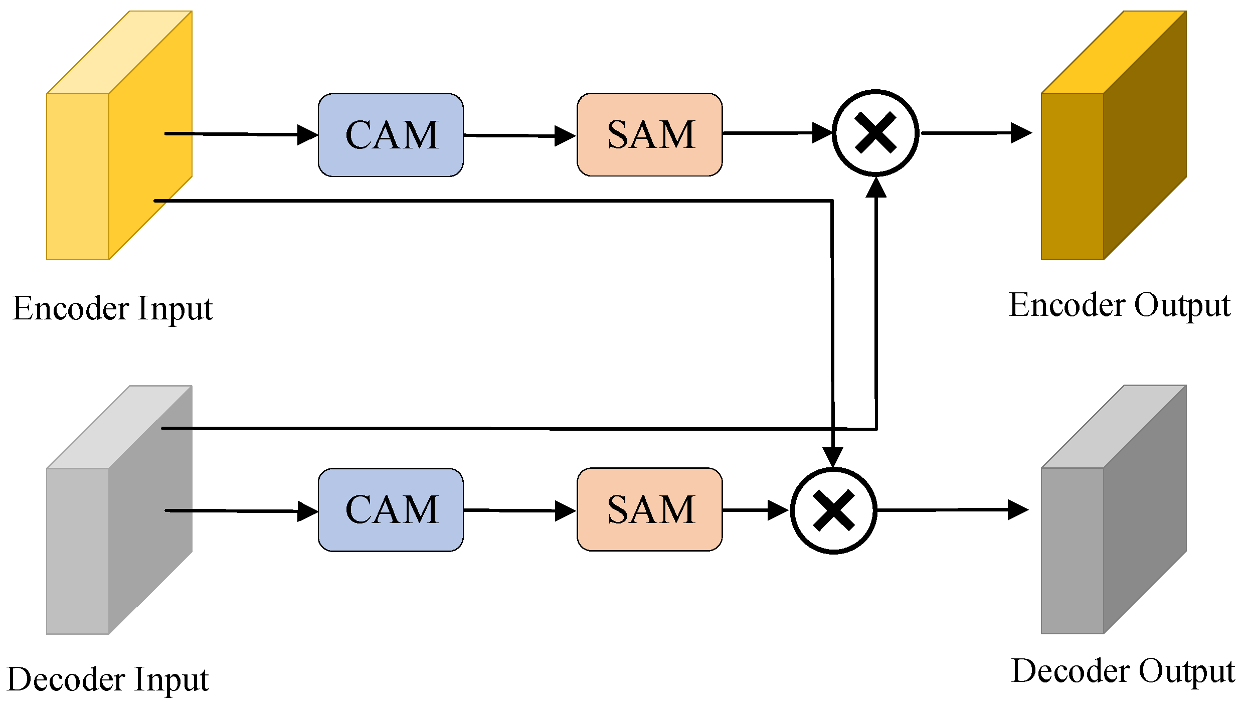
• Cross-guide module (CGM): In the CG-UNet algorithm, we innovatively introduced the cross-guide module. This module optimizes the upsampling process of images by introducing guidance information in the crosslayer connection between the encoder and decoder, thereby achieving high-precision edge restoration.
• Joint loss function: We designed a novel joint loss function that combines local and global information, significantly improving the model’s ability to discriminate pixels near edges. The design of this loss function makes our model more robust when dealing with easily confused pixels.
• Edge detection network with encoding and decoding structure: We designed an efficient encoding and decoding structure network for detecting ice thickness. The experimental results for the ice cover dataset show that the network can achieve an edge detection accuracy (ODS) of 0.934 and an edge recognition accuracy (OIS) of 0.938, with a thickness detection error controlled within 7.2%.

2. Related Works

Edge detection, a fundamental task in computer vision, has evolved over 40 years, giving rise to numerous classic recognition algorithms. Traditional methods for edge detection involve manual rule design based on features such as texture [19]. Initially, researchers computed the image gradient to extract edge information using methods such as Sobel [20], Robert [21], Laplacian [22], and the Canny operator [23]. Subsequently, learning-based approaches integrated these low-level features for enhanced edge detection. In recent years, deep learning has undergone substantial advancements, leading to the development of popular edge detection algorithms based on convolutional neural networks. Among these, HED [24] is the first to propose an end-to-end edge detection algorithm that aggregates feature maps from each branch to generate the final output, accompanied by a weighted cross-entropy loss function. RCF [25] further enhances feature fusion across convolutional layers to capture image information at multiple scales. LPCB [26] introduces an end-to-end network structure utilizing VGG as the backbone, integrating the dice loss function [27] and cross-entropy loss function. BDCN [28] introduces a bidirectional cascade network structure, wherein labeled edges supervise each layer at a specific scale; moreover, it introduces a scale enhancement module for multi-scale feature generation. DexiNed [29] presents a robust edge detection system combining HED with the Xception network [30]. PiDiNet [31] introduces a new pixel difference convolution, which integrates traditional edge detection operators into the convolution operation. UAED [32] exploits uncertainty to examine the subjectivity and ambiguity of different annotations in edge detection datasets, transforming the deterministic label space into a learnable Gaussian distribution whose variance measures the ambiguity between different annotations.

Edge detection algorithms can be used to detect the edges of ice-covered transmission lines. Liu et al. [33] used the Canny edge detection operator used for the aforementioned purpose, but its detection accuracy was not high. Chang et al. [34] used the ratio operator on ice cover infrared images to detect edges and calculate ice thickness. However, the ratio operator is sensitive to noise, which limits its practical application. Nusantika et al. [35] used a hybrid approach combining Gaussian and bilateral filters with the Canny operator for edge detection of ice-covered transmission lines, effectively improving detection accuracy, but the calculation process of ice thickness became more complex. Liang et al. [36] introduced a linear detection algorithm based on the LSD algorithm to detect ice thickness on transmission lines, but the detection effect is poor in complex backgrounds. Due to the limitations of manually designing features using traditional methods, the edge detection accuracy of these methods is not high, and they are highly sensitive to noise, resulting in poor performance in practical applications.

Lin et al. [37] proposed a robust generalized convolutional neural network for thickness detection of ice-covered transmission lines. They introduced the IBP algorithm to determine the number of convolutional layers and kernels. But its model training is relatively complex and requires the optimization of many parameters. Hu et al. [38] segmented the ice-covered area and the background area and trained a model for ice thickness detection using transfer learning with an attention mechanism. But it is not accurate enough in processing edge details, resulting in difficulty in feature recognition at the edges. Pi et al. [39] used image enhancement techniques to expand the dataset of ice-covered transmission lines and then directly identified the ice thickness of transmission lines using Mask RCNN network. However, due to the limitations of the object detection method used, it can only identify the ice thickness in the interval and cannot accurately identify the ice thickness. Ma et al. [40] proposed an IDR Net algorithm for extracting ice thickness on transmission lines, designed a multi-scale icing feature extraction module, and improved the traditional upsampling module. However, its detection performance was poor, and the model parameters were large. Nusantika et al. [41] utilized multi-stage image processing techniques and fused multi-scale adaptive Retinex to detect the ice thickness on transmission lines, but it was greatly affected by background and had poor scalability.

Table 1. Comparison of edge detection algorithms for ice-covered transmission lines.

Classification	Algorithm	Advantages and Disadvantages
Traditional edge detection algorithms	Canny	It can recognize simple edge information, but the overall detection accuracy is not high.
	Ratio	Capable of detecting multi-scale and multi-directional edge information, sensitive to noise.
	Improvement Canny	Improved the detection accuracy of the Canny operator, but the calculation process is more complex.
	LSD	The LSD algorithm is used for linear detection, but it performs poorly in complex backgrounds.
Deep learning detection algorithms	IBP	The use of IBP algorithm to determine the parameters of convolutional layers is a complex training process and difficult to optimize parameters.
	S_UNet	The use of transfer learning and attention mechanisms for ice-covered area segmentation is not precise enough for edge detail processing.
	Mask RCNN	The use of object detection technology for ice thickness recognition can only determine whether the ice thickness is within a certain range.

shows the advantages and disadvantages of traditional methods and deep learning methods.

At present, most methods for detecting the thickness of ice on ice-covered transmission lines still use traditional edge detection algorithms, which can only detect ice in scenes with relatively simple backgrounds and have poor detection performance. At present, deep learning methods for detecting ice cover thickness are promising for future development. However, current algorithms have not been specifically designed for the characteristics of ice-covered transmission lines, nor have they considered details such as ice-covered edges. At present, there is relatively little research on using deep learning edge detection algorithms for ice cover detection.

Although various edge detection algorithms have been applied to the detection of ice-covered transmission lines, there is currently a lack of deep learning edge detection algorithms specifically designed for the characteristics of ice-covered transmission lines. Ice cover has unique and complex characteristics, such as irregular shapes of ice edges, blurred boundaries between the ice layer and the background, and unstable features caused by changes in lighting conditions and different weather conditions. The existing algorithms have obvious limitations in processing these complex features, making it difficult to accurately distinguish between ice layers and backgrounds, and thus they are unable to accurately detect ice thickness. Taking traditional algorithms as an example, although the Canny operator can recognize simple edge information, its detection accuracy is less than 40% when facing ice-covered edges in complex backgrounds; although the ratio operator has the ability to detect multi-scale and multi-directional edge information, it is extremely sensitive to noise. In terms of deep learning algorithms, the IBP algorithm model training process is complex, parameter optimization is difficult, and it is not precise enough when dealing with details of ice-covered edges; the Mask RCNN network can only identify the approximate range of ice thickness and cannot accurately determine a specific numerical value. All of these highlight the necessity of developing new models. Therefore, we designed a neural network model suitable for edge detection of ice-covered transmission lines using edge detection methods, considering two aspects: network structure and loss function.

3. Cross-Guide-UNet (CG-UNet)

The CG-UNet edge detection model, illustrated in Figure 1, follows an encoder and decoder framework. In this model, the image of ice-covered power lines is input into the encoder to extract image features at various levels.

In CG-UNet, the encoder extracts different levels of features from the image through multi-layer convolution operations, including basic features such as color, texture, and shape. For example, in early convolutional layers, low-level features such as the edges and lines of the image are mainly extracted, which help the model to preliminarily identify the contours of transmission lines and ice; as the convolutional layer deepens, more advanced and abstract features are gradually extracted, such as the spatial relationship between the ice and transmission lines, providing rich information for subsequent ice edge detection and thickness calculation.

We implemented a CGM during decoding to facilitate interaction between information from different features. The features extracted by the encoder and decoder traverse the CGM, where calculated attention weights are derived. These weights are subsequently cross-multiplied with the input features to achieve deep-level feature fusion. Ultimately, the edge detection image is generated through multiple sampling modules.

3.1. Cross-Guide Module

Figure 2 shows a schematic of the CGM. The features extracted by the encoder are connected through crosslayers. Initially, channel attention is extracted, followed by the calculation of spatial attention. The calculated spatial attention utilized to weigh the decoder features guides the decoder’s image recovery process. Furthermore, the features extracted by the decoder undergo the same operation, and the cross-weighted features are concatenated to generate edge images.

$$Y_{en}={\Sigma }_{i=1}^n{A}_{de}^i\cdot X_{en}^i$$

(1)

Equation (1) is the calculation formula for encoder weighted attention. $A_{de}^i$ represents the weight calculated by the decoder through the attention module, and $X_{en}^i$ is the input feature of the encoder. The attention weights of all features were dot-multiplied with the feature vectors and combined to obtain the final encoder output feature $Y_{en}$.

$$Y_{de}={\Sigma }_{j=1}^n{A}_{en}^j\cdot X_{de}^j$$

(2)

Equation (2) is used to calculate the weighted attention of the decoder. $A_{en}^j$ is the feature attention weight of the encoder, and $X_{de}^j$ is the input feature of the decoder. Similarly to Equation (1), point multiplication is performed to obtain the output feature $Y_{de}$ of the decoder.

3.1.1. Channel Attention

Channel attention assesses the relation between feature maps. Figure 3 illustrates the diagram of channel attention. The channel attention utilized by the CGM differs from that of ECA-Net [42]. Initially, the feature maps undergo max and average pooling based on the spatial dimension to acquire spatial aggregation information for each channel. Max pooling tends to capture more prominent information particularly evident at pixel changes, such as edges. Subsequently, a one-dimensional convolution kernel is employed to compute the channel attention. Upon completion of the calculations, the results are summed to obtain complete channel attention and multiplied by the original feature map.

Equations (3) and (4) outline the calculation methods for channel attention.

$$\begin{array}{c}{W}_{ca}^i=\sigma {\Sigma }_{i=1}^n\left(C\right(M\left(X^i\right))+C(A\left(X^i\right)\left)\right)\end{array},$$

(3)

$$Y_{ca}^i=X^i\cdot W_{ca}^i+X^i,$$

(4)

$X^i$ is the input feature map. $M\left(X^i\right)$ represents applying max pooling operation to the input feature map, and $A\left(X^i\right)$ represents applying the average pooling operation to the input feature map. $C$ represents convolution operation, and $\sigma$ is the Sigmoid activation function.$W_{ca}^i$ is the calculated attention weight. Equation (4) multiplies $W_{ca}^i$ with point $X^i$ and performs residual connections to obtain the output, $Y_{ca}^i$.

3.1.2. Spatial Attention

ECA-Net solely utilizes channel attention and does not incorporate spatial attention. Spatial attention is pivotal for highlighting essential features within the image, particularly to help the model focus on the ice edge. Consequently, the CGM calculates spatial attention after extracting channel attention from the feature map. Figure 4 illustrates the diagram of spatial attention.

Spatial attention in the CGM draws inspiration from the calculation method of channel prior convolutional attention (CPCA) [43]. It employs a dynamic allocation method and replaces the convolution kernel with strip convolutions, rendering it more appropriate for strip images like transmission lines. Unlike channel attention, spatial attention does not aggregate feature maps in a specific direction since it assigns identical spatial attention information to all channels. This ensures the preservation of distinctions between various channels. Attention is computed through strip convolutions using convolution kernels of different scales. Finally, spatial attention weight is derived through addition.

$$Y_{sa}^i=C_1({\displaystyle {\sum }_{k=0}^3} B_k(C_{dw}(Y_{ca}^i))),$$

(5)

Equation (5) presents the formula expression of spatial attention. $Y_{ca}^i$ is the channel attention weighted image feature, $C_{dw}$ represents deep convolution, $B_k$ is the k-th branch, and $C_1$ represents the convolutional layer with kernel 1. By calculating the spatial attention of different branches, the final feature vector is obtained.

3.1.3. CGM

In previous edge detection algorithms, the fusion between the encoder and decoder was limited to simple splicing, failing to extract the relation between cascade features effectively. Hence, we designed a CGM. By computing the attention weights of the encoder and decoder and employing a cross-conferring mechanism, we enhanced the connection of cascade features, thereby effectively guiding the generation of edge images. The CGM not only achieves crosslayer interaction and fusion of encoder and decoder features but also weights and filters features at different levels through channel attention and spatial attention mechanisms, enabling the model to focus more on key features related to ice edges and enhancing feature representation capabilities.

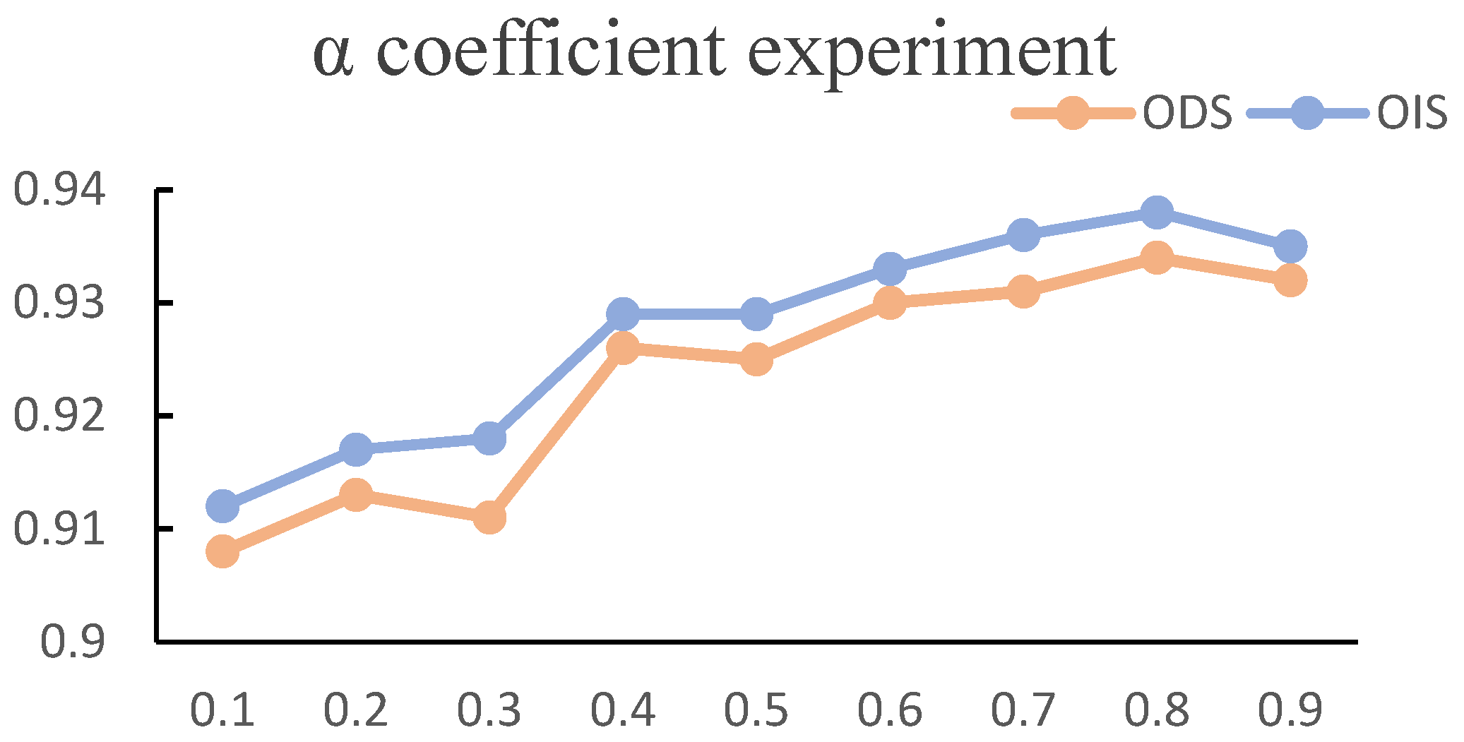
3.2. Joint Loss Function

In Section 3.1, the structure of the edge detection model is redesigned. Further, the loss function is crucial for ensuring detection accuracy. The edge detection loss function primarily comprises a weighted cross-entropy loss function, given as follows:

$$f_{ce}\left(G,P\right)=-W_i{\sum }_i^N \left(G_i\mathrm{l}\mathrm{o}\mathrm{g}{p}_i+\left(1-G_i\right)\log \left(1-p_i\right)\right),$$

(6)

where $G_i$ represents the real label value, $p_i$ represents the predicted value, $N$ represents the number of pixels, and $W_i$ represents the weight. The weighted cross-entropy loss function can be considered as a pixel-level loss calculation, comparing the predicted value of each pixel with the true value to compute the error and derive the loss. However, a single loss function fails to differentiate pixels near real edges effectively and often misclassifies non-edge pixels as edge pixels. The boundary difference over union (DoU) loss function [44] can be used to calculate the loss based on the boundary difference between predicted and true values, enabling focused attention on pixel information proximal to the edge. Distinct from weighted cross-entropy, the boundary DoU loss function can be viewed as an object-level loss calculation. The DoU loss is computed using Equation (7).

$$L_{DoU}={\displaystyle \frac{G\cup P-G\cap P}{G\cup P-\alpha *G\cap P}},$$

(7)

where $G$ represents the true value, $P$ represents the predicted value, and $\alpha$ is set to 0.8, controlling the width of the boundary calculation; the smaller the value, the more distance between the predicted boundary and the true boundary, and the lower the punishment intensity for prediction failure. On the contrary, it will increase the punishment intensity for prediction failure. We combined the weighted cross-entropy loss function and the boundary DoU loss function to create a joint loss function. While the weighted cross-entropy loss function emphasizes pixel differences, the boundary DoU loss function addresses overall differences. The joint loss is calculated using Equation (8).

$$L=L_{DoU}+\beta L_{CE},$$

(8)

The parameter $\beta$ is set to 0.001 to control the proportion of the loss function. The joint loss function optimizes the edge detection model from two distinct perspectives and effectively distinguishes pixels with high uncertainty near the real edge.

The joint loss function combines cross-entropy loss and boundary loss to perform differential constraints on different types of pixels during model training. Cross-entropy loss focuses on the classification accuracy of each pixel, while boundary loss focuses on optimizing the difference between predicted and true boundaries. The combination of the two effectively improves the model’s ability to distinguish ice edge pixels and reduces the occurrence of misjudgments.

4. Experimental Results and Analysis

4.1. Image Dataset

Owing to the absence of publicly available image datasets for ice-covered transmission lines, we opted to simulate the conditions of ice-covered transmission lines and build a dataset accordingly. We conducted icing experiments on transmission lines in a low-temperature laboratory, and the materials and specifications of the transmission lines used in the experiments were consistent with those of the actual transmission lines. During the experiment, we controlled the temperature, humidity, and other environmental parameters, and simulated natural icing by adjusting the release of water droplets from spray. Throughout the process, a camera was used to capture images of the ice-covered transmission line. The original image had a resolution of 4608 × 3456, and after adjustment, we uniformly scaled it to 512 × 512. After strict screening and cleaning of the captured images, a dataset containing 304 images of iced transmission lines was finally obtained.

These images were then divided into training and test sets at a ratio of 9:1. The experimental setup involved the Pytorch 1.13.1 deep learning framework, an RTX 4090 GPU, and the Ubuntu 20.04.6 operating system. The batch size was set to 16, the learning rate was 0.001, and the EPOCH was 50 rounds.

4.2. Ablation Experiment

To assess the effectiveness of the proposed edge detection model, ablation experiments, comprising four sets of control experiments, were designed for comparison. “DoU Loss” denotes training using a joint loss function; “Attention” involves the addition of an attention mechanism at crosslayer connections; and “CGM” indicates the utilization of the cross-guide module. Edge detection was executed on the ice cover dataset, and the experimental results are presented in

Table 2. Ablation experiment results.

	DoU Loss	Attention	CGM	ODS	OIS
Baseline				0.907	0.917
CG-UNet	✓			0.924	0.929
		✓		0.922	0.928
	✓	✓		0.926	0.930
	✓	✓	✓	0.934	0.938

.

Table 2 illustrates that UNet, serving as the baseline, yielded the lowest experimental results. Training with the DoU loss function and the weighted cross-entropy loss function concurrently led to improvements in ODS and OIS by 1.7% and 1.2%, respectively, indicating the network’s ability to discern pixels near real edges. Incorporating the attention mechanism based on the UNet network model resulted in 1.5% and 1.1% enhancements in the two evaluation indicators. In the final set of control experiments, the cross-guide module enhanced the ODS performance index by 1.2% and the OIS performance index by 0.8%, affirming the CGM’s efficacy in guiding sampling image restoration. The experimental results in Table 2 clearly demonstrate the improvement effect of each component on CG UNet, which strongly proves that our improvement is effective for final edge detection.

4.3. DoU Loss Function Parameter Experiment

In DoU loss, there exists an alpha hyperparameter to control the proportion of boundary optimization. In order to obtain the optimal parameter values, we conducted an $\alpha$ coefficient experiment, and the experimental results are shown in Figure 5.

As shown in the above figure, when the value of α was small, the penalty effect of the loss function was not good, resulting in lower ODS and OIS. When the value was 0.9, the optimization space given to the model was relatively small, and the effect was not as good that at 0.8. Therefore, this study selected 0.8 as the value of α.

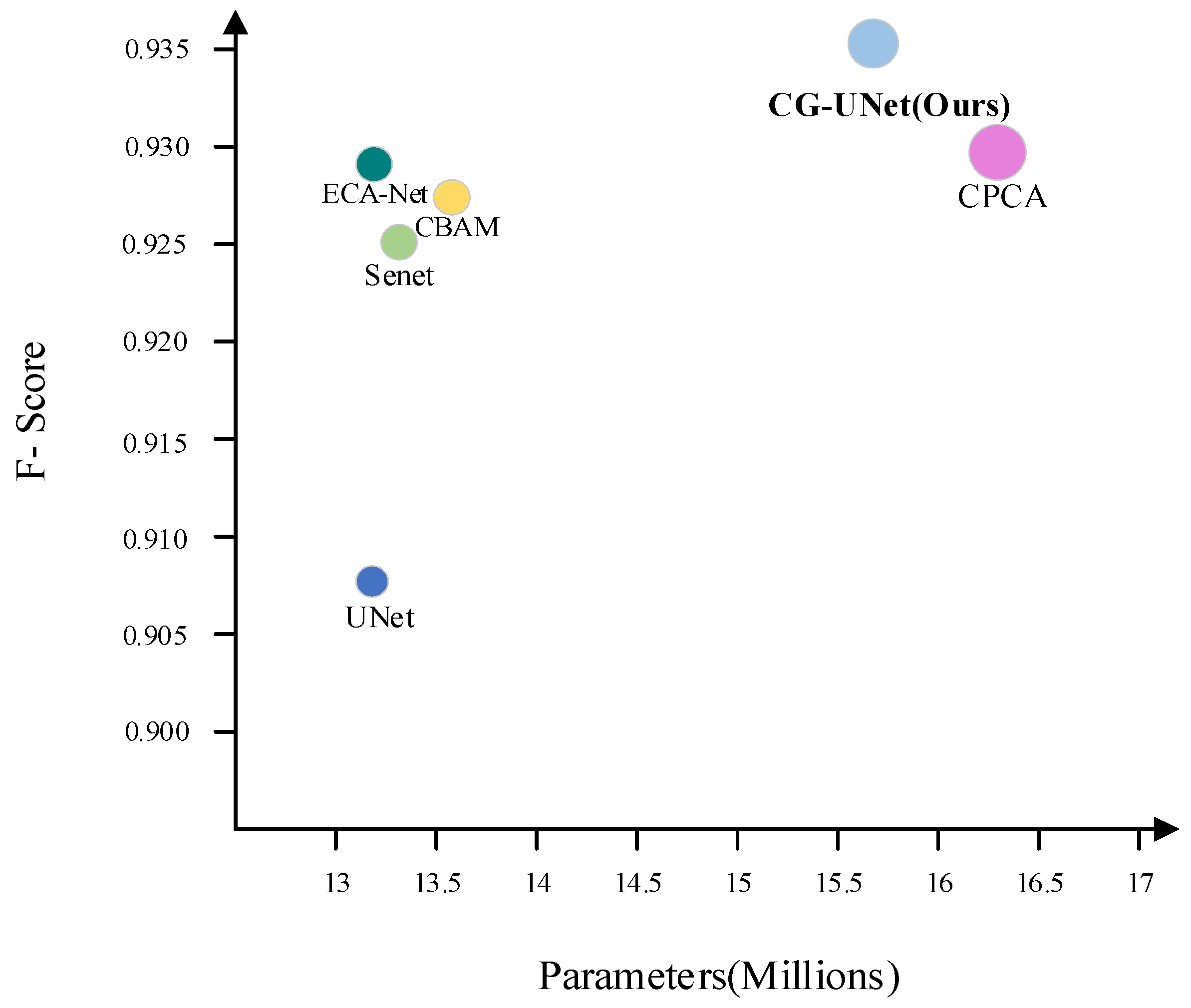
4.4. Attention Comparison Experiment

Due to our enhancements in attention, particularly based on ECA-Net, the effectiveness of the proposed attention module in this study was validated by comparing it with other attention modules. Senet [45], CBAM [46], ECA-Net, and CPCA attention were integrated into the model, and attention comparison experiments were conducted. The experimental results are depicted in Figure 6.

Figure 6 illustrates the experimental results of replacing our proposed attention module with other algorithms. Senet calculates channel attention through the fully connected layer. CBAM adds spatial attention based on Senet, resulting in a 0.2% increase in the F-score. ECA-Net substitutes the calculation of channel attention with efficient convolution operations, enhancing the model’s edge detection capabilities while reducing the number of parameters. CPCA enhances the model’s attention to spatial content by separately extracting spatial attention from features weighted by channel attention. The attention module proposed in this study, which is based on ECA-Net and incorporates the advantages of the above attention modules, achieved the most favorable recognition results, with the F-score reaching 0.934. Moreover, the parameters of CG-UNet were superior to those of CPCA, being reduced by 0.7 M.

4.5. Comparison with Other Algorithms

Edge detection is a fundamental task in computer vision, with numerous exemplary detection models emerging in recent years. In this section, we juxtapose the detection effects of other edge detection algorithms on the ice cover dataset with our proposed CG-UNet. The experimental results are delineated in

Table 3. Comparison of results with other algorithms.

Method	ODS	OIS	Parameter/M	GFLOPS	FPS
Canny	0.323	0.323	-	-	-
HED	0.858	0.867	14.7	93.5	34.8
RCF	0.873	0.883	14.8	102.6	33.4
BDCN	0.900	0.905	16.3	143.6	25.6
DexiNed	0.901	0.912	35.1	140.4	21.2
PidiNet	0.912	0.920	11.4	78.2	38
UAED	0.924	0.927	9.1	97.3	26.3
CG-UNet	0.934	0.938	15.8	156.7	24.5

.

As depicted in Table 3, Canny, the sole non-deep-learning algorithm, exhibited the poorest detection performance and proved ineffective in discerning ice-covered edges within complex environments. Other deep learning algorithms attained a recognition accuracy of 85%. Notably, the CG-UNet model demonstrated substantial advantages over other edge detection algorithms, owing to the incorporation of the CGM and joint loss function. Due to the CGM, the CG-UNet has more parameters than other models, but its detection speed has not decreased significantly, maintaining above 20 FPS on the RTX3050 GPU. Figure 7 provides a visual representation of the performance of various algorithms on the ice-covered transmission line dataset.

As depicted in Figure 7, the edges in the image generated by RCF appeared thicker, and the pixels within the bumps were not effectively processed. PidiNet, after redesigning the convolution operator and integrating traditional methods, achieved initial differentiation of pixels near real edges. Conversely, CG-UNet excelled in detecting uneven areas, particularly with the aid of the CGM. This module enables the model to effectively leverage encoder features to distinguish easily confused pixels during edge generation. Moreover, the joint loss function contributes to thinner edge generation.

4.6. Calculation of Ice Thickness

Upon detecting the edge of the ice-covered transmission line, the predicted ice thickness can be computed by analyzing the pixel difference between the upper and lower edges of the image. The ice-covered edge can be predicted by selecting four ice-covered transmission lines with varying thicknesses. Figure 8 illustrates the results of ice-covered edge prediction.

Once the edge map of the ice-covered transmission line is acquired, the calculation of the ice thickness proceeds as follows:

$$h={\displaystyle \frac{d_2-d_1}{2}}\times {\displaystyle \frac{D_1}{d_1}},$$

(9)

where $D_1$ represents the actual diameter of the transmission line, $d_1$ represents the pixel width of the upper and lower boundary outlines of the ice-free transmission line image, $d_2$ represents the pixel width of the upper and lower boundary outlines of the ice-covered line image. Among them, $D_1$ and $d_1$ are pre-known parameters, through which we can obtain the correspondence between pixel width and actual size. Then, by comparing the pixel difference between the upper and lower boundaries with and without ice cover, we can obtain the actual ice cover thickness. The experimental results are displayed in

Table 4. Ice thickness calculation results.

Actual Thickness/mm	Test Method	Predicted Thickness/mm	Error
5.0	CG-UNet	4.64	0.072
	UAED	4.53	0.094
	S-UNet	5.76	0.152
11.0	CG-UNet	11.52	0.047
	UAED	10.33	0.061
	S-UNet	11.86	0.078
17.5	CG-UNet	16.90	0.034
	UAED	18.34	0.048
	S-UNet	16.62	0.050
20.5	CG-UNet	21.96	0.071
	UAED	22.34	0.089
	S-UNet	18.73	0.086

.

As illustrated in Table 4, the ice thickness detected by the CG-UNet model through edge computation exhibited a maximum error of 7.2% and a minimum error of 3.4%. Compared to UAED and S-UNet, our model had smaller recognition errors for both thin and thick ice cover. The overall error fell within a controllable range, affirming the CG-UNet model’s capability to detect ice cover thickness on transmission lines.

5. Conclusions

This study delved into the detection of ice thickness on transmission lines and introduced a model tailored for edge detection of ice-covered lines. The main contribution of this study is the innovation concerning network structure and loss function. Regarding the network structure, the traditional encoder and decoder configuration was revamped using CG-UNet, wherein a cross-guide module was added at the crosslayer connection to guide the decoder to generate edge images with higher accuracy. Based on ECA-Net, the CGM undergoes targeted enhancements in channel and spatial attention, rendering it more adept at calculating strip-shaped objects. Further, a joint loss function is proposed, combining the weighted cross-entropy loss function with the DoU loss function to effectively discern pixels with high uncertainty near the true edge. Subsequently, experimental validation was conducted on the ice cover dataset, yielding an ODS of 0.934 and an OIS of 0.938. Moreover, the calculation error for ice thickness remained within 7.2%.

Considering the weak computing power of edge devices, the CG-UNet model was not designed to be lightweight, resulting in its detection speed being unable to achieve real-time detection accuracy. There are still areas that can be optimized in regard to real-time detection, which is the direction for our future research. In practical scenarios, transmission lines do not remain stationary and often sway in the wind, making it difficult to use image detection methods for calculating ice thickness. The next phase involves designing a suitable image detection algorithm that accommodates the oscillating nature of transmission lines, aiming to enhance the accuracy of ice thickness calculations. In addition, we plan to collect more images of ice-covered transmission lines in actual environments, which will be used to train and validate our model to ensure its accuracy and robustness in practical applications.

References

1. Yang, L.; Chen, J.; Hao, Y.; Li, L.; Lin, X.; Yu, L.; Li, Y.; Yuan, Z. Experimental study on ultrasonic detection method of ice thickness for 10 kV overhead transmission lines. IEEE Trans. Instrum. Meas. 2023, 72, 1–10. [Google Scholar] [CrossRef]
2. Zhang, C.; Gong, Q.; Koyamada, K. Visual analytics and prediction system based on deep belief networks for icing monitoring data of overhead power transmission lines. J. Vis. 2020, 23, 1087–1100. [Google Scholar] [CrossRef]
3. Huang, J.; Zhou, X. Study on transmission line icing prediction based on micro-topographic correction. AIP Adv. 2022, 12, 085103. [Google Scholar] [CrossRef]
4. Yang, G.; Jiang, X.; Liao, Y.; Li, T.; Deng, Y.; Wang, M.; Hu, J.; Ren, X.; Zhang, Z. Research on load transfer melt-icing technology of transmission lines: Its critical melt-icing thickness and experimental validation. Electr. Power Syst. Res. 2023, 221, 109409. [Google Scholar] [CrossRef]
5. Zhu, Y.; Tan, Y.; Huang, Q.; Huang, F.; Zhu, S.; Mao, X. Research on melting and de-icing methods of lines in distribution network 3rd Conference on Energy Internet and Energy System Integration. In Proceedings of the 2019 IEEE 3rd Conference on Energy Internet and Energy System Integration (EI2), Changsha, China, 8–10 November 2019; IEEE: Piscataway, NJ, USA, 2020; pp. 2370–2373. [Google Scholar] [CrossRef]
6. Ma, T.; Fu, W.G.; Ma, J. Popliteal vein external banding at the valve-free segment to treat severe chronic venous insufficiency. J. Vasc. Surg. 2016, 64, 438–445.e1. [Google Scholar] [CrossRef]
7. Fikke, S.M.; Kristjánsson, J.E.; Kringlebotn Nygaard, B.E. Modern Meteorology and Atmospheric Icing Atmospheric Icing of Power Networks; Springer: Berlin/Heidelberg, Germany, 2008; pp. 1–29. [Google Scholar] [CrossRef]
8. Zhong, J.; Jiang, X.; Zhang, Z.; Zhu, Z.; Wu, Z.; Liu, X. Equivalent measurement method for ice thickness of transmission lines. J. Phys. Conf. Ser. 2024, 2896, 012033. [Google Scholar] [CrossRef]
9. Yang, L.; Chen, Y.; Hao, Y.; Li, L.; Li, H.; Huang, Z. Detection method for equivalent ice thickness of 500-kV overhead lines based on axial tension measurement and its application. IEEE Trans. Instrum. Meas. 2023, 72, 1–11. [Google Scholar] [CrossRef]
10. Yao, C.G.; Zhang, L.; Li, C.X. Measurement method of conductor ice covered thickness based on analysis of mechanical and sag measurement. High Volt. Eng. 2013, 39, 1204–1209. [Google Scholar] [CrossRef]
11. Berlijn, S.M.; Gutman, I. Laboratory tests and web based surveillance to determine the ice-and snow performance of insulators. IEEE Trans. Dielectr. Electr. Insul. 2007, 14, 1373–1380. [Google Scholar] [CrossRef]
12. Wang, J.; Wang, J.; Shao, J.; Li, J. Image recognition of icing thickness on power transmission lines based on a least squares Hough transform. Energies 2017, 10, 415. [Google Scholar] [CrossRef]
13. Verma, R.; Kumar, N.; Patil, A. MoNuSAC2020: A multi-organ nuclei segmentation and classification challenge. IEEE Trans. Med. Imaging 2021, 40, 3413–3423. [Google Scholar] [CrossRef] [PubMed]
14. Zunair, H.; Hamza, A.B. Sharp U-Net: Depthwise convolutional network for biomedical image segmentation. Comput. Biol. Med. 2021, 136, 104699. [Google Scholar] [CrossRef] [PubMed]
15. Zunair, H.; Hamza, A.B. Masked supervised learning for semantic segmentation. arXiv 2022, arXiv:2210.00923. [Google Scholar] [CrossRef]
16. Varshney, D.; Rahnemoonfar, M.; Yari, M.; Paden, J. Deep ice layer tracking and thickness estimation using fully convolutional networks. In Proceedings of the 2020 IEEE International Conference on Big Data (Big Data), Atlanta, GA, USA, 10–13 December 2020; IEEE: Piscataway, NJ, USA, 2020; pp. 3943–3952. [Google Scholar] [CrossRef]
17. Wang, B.; Ma, F.; Ge, L.; Ma, H.; Wang, H.; Mohamed, M.A. Icing-EdgeNet: A pruning lightweight edge intelligent method of discriminative driving channel for ice thickness of transmission lines. IEEE Trans. Instrum. Meas. 2020, 70, 1–12. [Google Scholar] [CrossRef]
18. Nusantika, N.R.; Hu, X.; Xiao, J. Newly designed identification scheme for monitoring ice thickness on power transmission lines. Appl. Sci. 2023, 13, 9862. [Google Scholar] [CrossRef]
19. Xiao, Y.; Zhou, J. Overview of image edge detection. Comput. Eng. Appl. 2023, 59, 40–54. [Google Scholar] [CrossRef]
20. Kittler, J. On the accuracy of the Sobel edge detector. Image Vis. Comput. 1983, 1, 37–42. [Google Scholar] [CrossRef]
21. Roberts, L.G. Machine Perception of Three-Dimensional Solids. Ph.D. Thesis, Massachusetts Institute of Technology, Cambridge, MA, USA, 1963. [Google Scholar]
22. Lecun, Y.; Bottou, L.; Bengio, Y.; Haffner, P. Gradient-based learning applied to document recognition. Proc. IEEE 1998, 86, 2278–2324. [Google Scholar] [CrossRef]
23. Canny, J. A computational approach to edge detection. IEEE Trans. Pattern Anal. Mach. Intell. 1986, 8, 679–698. [Google Scholar] [CrossRef]
24. Xie, S.; Tu, Z. Holistically-nested edge detection. In Proceedings of the IEEE International Conference on Computer Vision, Santiago, Chile, 7–13 December 2015; pp. 1395–1403. [Google Scholar] [CrossRef]
25. Liu, Y.; Cheng, M.M.; Hu, X.; Wang, K.; Bai, X. Richer convolutional features for edge detection. In Proceedings of the IEEE Conference on Computer Vision and Pattern Recognition, Honolulu, HI, USA, 21–26 July 2017; pp. 3000–3009. [Google Scholar] [CrossRef]
26. Deng, R.; Shen, C.; Liu, S. Learning to predict crisp boundaries. In Proceedings of the European Conference on Computer Vision (ECCV), Munich, Germany, 8–14 September 2018; pp. 562–578. [Google Scholar] [CrossRef]
27. Milletari, F.; Navab, N.; Ahmadi, S.A. V-net: Fully convolutional neural networks for volumetric medical image segmentation. In Proceedings of the 2016 Fourth International Conference on 3D Vision (3DV), Stanford, CA, USA, 25–28 October 2016; IEEE: Piscataway, NJ, USA, 2016; pp. 565–571. [Google Scholar] [CrossRef]
28. He, J.; Zhang, S.; Yang, M.; Shan, Y.; Huang, T. Bi-directional cascade network for perceptual edge detection. In Proceedings of the IEEE/CVF Conference on Computer Vision and Pattern Recognition, Long Beach, CA, USA, 15–20 June 2019; pp. 3823–3832. [Google Scholar] [CrossRef]
29. Poma, X.S.; Riba, E.; Sappa, A. Dense extreme inception network: Towards a robust cnn model for edge detection. In Proceedings of the IEEE/CVF Winter Conference on Applications of Computer Vision, Village, CO, USA, 1–5 March 2020; pp. 1923–1932. [Google Scholar] [CrossRef]
30. Chollet, F.; Xception, C.F. Deep learning with depthwise separable convolutions. In Proceedings of the IEEE Conference on Computer Vision and Pattern Recognition, Honolulu, HI, USA, 21–26 July 2017; pp. 1251–1258. [Google Scholar] [CrossRef]
31. Su, Z.; Liu, W.; Yu, Z.; Hu, D.; Liao, Q.; Tian, Q.; Pietikainen, M.; Liu, L. Pixel difference networks for efficient edge detection. In Proceedings of the IEEE/CVF International Conference on Computer Vision, Montreal, BC, Canada, 11–17 October 2021; pp. 5097–5107. [Google Scholar] [CrossRef]
32. Zhou, C.; Huang, Y.; Pu, M. The treasure beneath multiple annotations: An uncertainty-aware edge detector. In Proceedings of the IEEE/CVF Conference on Computer Vision and Pattern Recognition, Vancouver, BC, Canada, 17–24 June 2023; pp. 15507–15517. [Google Scholar] [CrossRef]
33. Liu, Y.; Tang, Z.; Xu, Y. Detection of ice thickness of high voltage transmission line by image processing. In Proceedings of the 2017 IEEE 2nd Advanced Information Technology, Electronic and Automation Control Conference (IAEAC), Chongqing, China, 25–26 March 2017; IEEE: Piscataway, NJ, USA, 2017; pp. 2191–2194. [Google Scholar] [CrossRef]
34. Chang, Y.; Yu, H.; Kong, L. Study on the calculation method of ice thickness calculation and wire extraction based on infrared image. In Proceedings of the 2018 IEEE International Conference on Mechatronics and Automation (ICMA), Changchun, China, 5–8 August 2018; IEEE: Piscataway, NJ, USA, 2018; pp. 381–386. [Google Scholar] [CrossRef]
35. Nusantika, N.R.; Hu, X.; Xiao, J. Improvement canny edge detection for the UAV icing monitoring of transmission line icing. In Proceedings of the 2021 IEEE 16th Conference on Industrial Electronics and Applications (ICIEA), Chengdu, China, 1–4 August 2021; IEEE: Piscataway, NJ, USA, 2021. [Google Scholar] [CrossRef]
36. Liang, S.; Wang, J.; Chen, P.; Yan, S.; Huang, J. Research on image recognition technology of transmission line icing thickness based on LSD Algorithm. In International Conference in Communications, Signal Processing, and Systems; Springer: Berlin/Heidelberg, Germany, 2020; pp. 100–110. [Google Scholar] [CrossRef]
37. Lin, G.; Wang, B.; Yang, Z. Identification of icing thickness of transmission line based on strongly generalized convolutional neural network. In Proceedings of the 2018 IEEE Innovative Smart Grid Technologies-Asia (ISGT Asia), Singapore, 22–25 May 2018; IEEE: Piscataway, NJ, USA, 2018. [Google Scholar] [CrossRef]
38. Hu, T.; Shen, L.; Wu, D.; Duan, Y.; Song, Y. Research on transmission line ice-cover segmentation based on improved U-Net and GAN. Electr. Power Syst. Res. 2023, 221, 109405. [Google Scholar] [CrossRef]
39. Ma, F.; Wang, B.; Li, M.; Dong, X.; Mao, Y.; Zhou, Y.; Ma, H. An Edge Intelligence Approach for Power Grid Icing Condition Detection through Multi-Scale Feature Fusion and Model Quantization. Front. Energy Res. 2021, 9, 754335. [Google Scholar] [CrossRef]
40. Ma, T.; Yuan, X.; Liu, R.; Wang, Z.; Liu, X. A deep learning-based method for extracting ice cover on power transmission lines. In Proceedings of the Fifth International Conference on Computer Vision and Data Mining (ICCVDM 2024), Changchun, China, 19–21 July 2024; SPIE: Bellingham, WA, USA, 2024; Volume 13272, pp. 707–713. [Google Scholar]
41. Nusantika, N.R.; Xiao, J.; Hu, X. Precision Ice Detection on Power Transmission Lines: A Novel Approach with Multi-Scale Retinex and Advanced Morphological Edge Detection Monitoring. J. Imaging 2024, 10, 287. [Google Scholar] [CrossRef]
42. Wang, Q.; Wu, B.; Zhu, P.; Li, P.; Zuo, W.; Hu, Q. ECA-Net: Efficient channel attention for deep convolutional neural networks. In Proceedings of the IEEE Conference on Computer Vision and Pattern Recognition, Seattle, WA, USA, 14–19 June 2020; IEEE Press: Piscataway, NJ, USA, 2020; pp. 11531–11539. [Google Scholar] [CrossRef]
43. Huang, H.; Chen, Z.; Zou, Y. Channel prior convolutional attention for medical image segmentation. arXiv 2023, arXiv:2306.05196. [Google Scholar] [CrossRef]
44. Sun, F.; Luo, Z.; Li, S. Boundary difference over union loss for medical image segmentation. In International Conference on Medical Image Computing and Computer-Assisted Intervention; Springer Nature: Cham, Switzerland, 2023; pp. 292–301. [Google Scholar] [CrossRef]
45. Hu, J.; Shen, L.; Sun, G. Squeeze-and-excitation networks. In Proceedings of the IEEE Conference on Computer Vision and Pattern Recognition, Salt Lake City, UT, USA, 18–22 June 2018; pp. 7132–7141. [Google Scholar] [CrossRef]
46. Woo, S.; Park, J.; Lee, J.Y. Cbam: Convolutional block attention module. In Proceedings of the European Conference on Computer Vision (ECCV), Munich, Germany, 8–14 September 2018; pp. 3–19. [Google Scholar] [CrossRef]
Figure 1. CG-UNet model structure.
Applsci 15 04264 g001
Figure 2. Cross-guide module.
Applsci 15 04264 g002
Figure 3. Diagram of channel attention.
Applsci 15 04264 g003
Figure 4. Diagram of spatial attention.
Applsci 15 04264 g004
Figure 5. α   coefficient experiment results.
Applsci 15 04264 g005
Figure 6. Attention comparison results.
Applsci 15 04264 g006
Figure 7. Edge detection visualization diagram: (a) original image and (b) ground truth. (c) RCF image, (d) PidiNet image, and (e) CG-UNet image.
Applsci 15 04264 g007
Figure 8. Ice edge prediction results: (a) 35 mm image, (b) 47 mm image, (c) 60 mm image, and (d) 66 mm image.
Applsci 15 04264 g008