Resource-Efficient Traffic Classification Using Feature Selection for Message Queuing Telemetry Transport-Internet of Things Network-Based Security Attacks

Abstract

The rapid proliferation of IoT devices necessitates robust security measures to protect against malicious traffic. Anomaly detection, primarily through traffic classification supported by artificial intelligence and machine learning techniques, has emerged as a practical approach to enhancing IoT network security. Effective traffic classification requires efficient feature selection, which is critical for resource-constrained IoT devices with limited computational power, memory, and energy. This study proposes Statistical Moments Difference Thresholding, a feature selection method leveraging statistical central moments to identify significant features distinguishing between legitimate and malicious traffic. The aim is to reduce feature dimensionality while maintaining high detection accuracy. Validated on the MQTTset dataset through binary and multiclass classification using seven ML algorithms, the results highlight its ability to enhance computational efficiency without compromising performance, showcasing its potential in real-world IoT security applications.

1. Introduction

Technological advances like the Internet of Things (IoT) continue to revolutionize various industries. IoT enables seamless connectivity and automation, facilitating the interconnection of devices for real-time data exchange and intelligent decision-making [1]. IoT networking protocols are essential to ensure that devices interact efficiently and effectively within an IoT network. The standard protocols utilized in IoT include but are not limited to Message Queuing Telemetry Transport (MQTT) protocol, Constrained Application Protocol (CoAP), Advanced Message Queuing Protocol (AMQP), and Hypertext Transfer Protocol/Secure (HTTP/HTTPS) [2,3,4,5]. Each protocol is applied to its most suitable IoT application based on specific requirements such as power consumption, bandwidth, and security [2,3].

MQTT, in particular, has gained widespread adoption in IoT applications due to its lightweight and efficient publish–subscribe architecture, establishing itself as a de facto standard for data transmission [6,7,8]. MQTT’s adaptability is demonstrated in many IoT applications, from smart home systems to industrial automation, healthcare monitoring, automotive, manufacturing, and telecommunications [9]. It is particularly prevalent in applications requiring reliable and low-latency communication [10], and the remote access feature further enhances its value in these applications [6,9].

Despite its advantages, MQTT is not without its limitations. Its lightweight design, while beneficial for resource-constrained IoT devices, does not inherently provide built-in security mechanisms (e.g., encryption, authentication, authorization) [5,10]. The responsibility for implementing appropriate security features is left to the implementor [6]. However, that approach has practical limitations. Several studies highlight that attempts to address these security gaps, such as employing transport layer security (TLS) for encryption and OAuth for authentication, add complexity and computational overhead to the system [7,8]. Consequently, researchers have found that many users deploy MQTT brokers over the default TCP port 1883 (unencrypted connections) instead of MQTT over SSL/TLS port 8883, which is a secure alternative [8,11].

These shortcomings pose significant security challenges. The MQTT-based IoT system is susceptible to various security threats and attacks, compromising the safety and integrity of data transmitted across the network. Some prevalent MQTT threats include unauthorized access, data tampering, information exposure, escalation of privileges, broker software vulnerabilities, attacks such as man-in-the-middle (MitM), denial of service (DoS), replay, and brute force attacks [4,7,12,13]. For instance, without encryption, attackers can intercept and alter data transmitted between devices and the broker in man-in-the-middle attacks. The reliance on a central broker in MQTT also introduces a single point of failure and a potential attack target [10]. With DoS, attackers overwhelm the broker with an excessive number of connections or messages, causing legitimate clients to be denied service. A compromised broker can lead to significant data loss, service interruptions, and even control over the connected IoT devices, posing severe risks to both safety and functionality. Moreover, the remote access capabilities amplify the attack surface [14]. Exposing remote services is a common attack vector in industrial environments [15]. Attackers can exploit security flaws, such as misconfigurations or weak credentials, in these services to gain unauthorized access.

Given the vulnerabilities inherent in MQTT-based IoT networks, exploring effective methods for detecting and mitigating security threats is imperative. Anomaly detection, mainly through traffic classification backed by artificial intelligence (AI)/machine learning (ML) techniques, has garnered significant attention as a practical and promising approach for enhancing network security in this context [4,5,16]. Effective traffic classification, however, requires efficient feature selection (FS). FS helps identify the most informative features, thereby reducing the amount of data that needs to be stored and processed, simplifying the model and making it more efficient [17]. FS becomes even more critical in the context of resource-constrained devices, such as those commonly found in IoT networks. IoT devices often have limited computational power, memory, and energy resources. Thus, it is essential to minimize the computational overhead to ensure real-time processing and extend the operational lifespan of these devices [18]. Moreover, traditional ML models are computationally intensive, often requiring substantial processing power and memory. Hence, efficient FS and dimensionality reduction not only improve the selection of the most discriminative features but also enable the deployment of more lightweight ML models on devices with limited capabilities without compromising performance or resource availability [18,19].

The contributions of this paper are summarized as follows:

-

We propose Statistical Moments Difference Thresholding (SMDT), a feature selection method that leverages four statistical central moments (mean, standard deviation, skewness, and kurtosis) to select the most significant features. To our knowledge, this is the first approach to leverage these specific statistical moments for FS, particularly in the context of IoT network security. The aim is to reduce feature dimensionality while maintaining a decent detection accuracy, particularly in resource-constrained environments.

-

We validate the proposed FS method on the MQTTset [20] dataset and evaluate the performance of seven ML models in detecting malicious traffic using the selected features, demonstrating its practicality and effectiveness.

-

We compare the effectiveness of binary and multiclass classification approaches, providing a comprehensive analysis of each method’s advantages and limitations.

-

We analyze the trade-offs between model accuracy, computational cost, and feature dimensionality, highlighting the balance between performance and efficiency.

The rest of this paper is structured as follows. Section 2 briefly reviews related work. Section 3 discusses the dataset utilized in our experiment, the preprocessing and exploratory data analysis methods used, and feature selection for malicious traffic classification, focusing on the method and criteria employed in our study to identify the most significant features. Section 4 presents the experiments conducted and the results obtained. Section 5 discusses these results and their implications, limitations, and future work. Finally, Section 6 provides concluding remarks.

2. Related Work

In this section, we provide a brief overview of recent works on IoT security, with a particular emphasis on methods to secure the MQTT protocol. Several studies have been conducted on this subject matter, and anomaly detection using ML has gained traction as a method for identifying malicious traffic within MQTT-based IoT networks.

For instance, the authors in [21] proposed an intelligent and lightweight detection scheme to identify low-rate distributed denial of service (LR-DDoS) attacks in a software-defined IoT environment. Their approach leveraged ML models to analyze traffic patterns and distinguish between legitimate and malicious activities. Their research evaluated the performance of four different machine learning models utilizing the LRDDoS-MQTT-2022 dataset: Decision Tree Classifier (DTC), Multilayer Perceptron (MLP), Artificial Neural Networks (ANNs), and Naive Bayes classifier (NBC). The authors demonstrated that the Decision Tree Classifier achieves an impressive accuracy of 99.5%, outperforming other models regarding prediction rates and detection speed.

Hindy et al. [22] introduced a simulated dataset, MQTT-IoT-IDS2020, which includes benign and attack instances, to train and evaluate the models. Their research evaluated six machine learning models: Decision Tree (DT), Random Forest (RF), k-nearest Neighbor (KNN), Naive Bayes (NB), Support Vector Machine (SVM), and Multilayer Perceptron (MLP). The authors analyzed packet-based, unidirectional, and bidirectional flow features to assess model performance. Their findings suggest that flow-based features provide better detection capabilities than packet-based features for MQTT-specific attacks.

The study presented in [16] focuses on enhancing the security of IoT systems that utilize the MQTT protocol through multiclass classification techniques. The authors employed both ensemble methods and deep learning (DL) models, specifically recurrent neural networks (RNNs), to classify attack types. The study used a dataset containing frames under attack within an IoT system using the MQTT protocol. The authors demonstrated that RRNs, in particular, provide satisfactory results in identifying various attack types, which is essential for developing robust intrusion detection systems (IDSs). However, the study did not address the computational complexity of deploying DL models, such as RNNs, on resource-constrained IoT devices. While these models exhibit high accuracy, their computational demands could pose significant challenges for real-time deployment and operation in environments with limited processing power and memory capacity.

Vaccari et al. [23] introduced the MQTTset dataset, which includes legitimate traffic and various cyber-attacks against MQTT networks. To validate the dataset, the authors employed various ML algorithms, such as NB, MLP, RF, GB, NN, and DT, to identify security threats. However, while the MQTTset dataset is a valuable resource, the methodology used to evaluate it needs improvement. Firstly, the authors did not employ feature reduction techniques. Feature reduction is crucial in machine learning as it helps simplify models, reduce overfitting, and improve computational efficiency. Secondly, the study did not involve hyperparameter tuning. Hyperparameter tuning is essential for optimizing machine learning models, as it consists of selecting the best set of parameters that maximize the model’s performance. While they achieved high accuracy, without this step, the models used in the study may have not been operating at their full potential.

Zeghida et al. [5] adapted the MQTTset dataset for binary classification. They proposed an IDS based on ensemble learning (EL) methods, explicitly bagging, boosting, and stacking. These methods involve training multiple machine learning models independently on random subsets of the training data and then combining their predictions to improve overall performance. Their study found that ensemble learning, mainly stacking models, offered significant improvements in accuracy, F1-score, and Matthew’s correlation coefficient (MCC) compared to individual ML models. Like the approach by Vaccari et al. [23], Zeghida et al. [5] did not incorporate feature reduction techniques or apply hyperparameter tuning to optimize the performance of their ML models.

Similarly, the study in [4] utilized MQTTset for binary classification. The authors employed feature selection methods to identify the most relevant features, enhancing the detection efficiency of an IDS. With the Pearson correlation coefficient (PCC) feature selection technique, they identified the top ten relevant features, significantly improving detection accuracy while reducing computational complexity. They evaluated multiple ML models, including Decision Tree, Random Forest, KNN, AdaBoost, and XGBoost, achieving high performance compared to previous studies utilizing the same dataset.

As previously discussed, our study extends existing research by introducing SMDT, a feature selection method that leverages statistical central moments to identify significant features distinguishing between legitimate and malicious traffic. By focusing on these statistical moments, SMDT aims to reduce feature dimensionality while maintaining high detection accuracy. This approach addresses the limitations of traditional feature selection methods, particularly in resource-constrained IoT devices, by ensuring efficient performance without compromising resource availability.

Table 1. Summary of the studies that utilized MQTTset.

Study	Year	Classifi- cation	ML Method	DL Method	Evaluation Metrics	FS Method	Retained Features	Hyperpara- meter Tuning	Cross- Validation
[23]	2020	Multi- class	RF, NB, DT, GB, MLP	DNN	Accuracy, F1-score	✗	33	✗	✗
[5]	2023	Binary	DT, RF, NB, MLP, Bagging, Adaboost, HGBoost, XGBoost, stacking	✗	Accuracy, F1-score, MCC	✗	33	✗	✗
[4]	2024	Binary	DT, KNN, RF, Adaboost, XGBoost	✗	Accuracy, Precision, Recall, F1-score, ROC	PCC	10	✓	✓
This study	2025	Binary and Multi- class	RF, LR, DT, GB, XGBoost, MLP	DNN	Accuracy, Precision, Recall, F1-score, ROC-AUC	SMDT	5	✓	✓

summarizes the previous studies utilizing the MQTTset dataset. Figure 1 presents the proposed method’s framework for feature selection and classification. This framework serves as the basis for the implementation discussed in the subsequent sections.

3. Materials and Methods

This section discusses the dataset utilized in our experiments. Additionally, we discuss the preprocessing and exploratory data analysis techniques applied to clean and structure the data and understand the underlying patterns and characteristics of the dataset. Moreover, we describe the tools and computational environment employed in our research, which are critical for reproducibility. Furthermore, we discuss feature selection for malicious traffic classification, focusing on the method and criteria employed in our study to identify the most discriminative features that contribute to dimensionality reduction while maintaining optimal performance.

3.1. Employed Dataset

Our study utilizes the MQTTset, a publicly available IoT dataset focused on MQTT communications, as described in [23] and available online [20]. The dataset is built using IoT sensors that operate on the MQTT protocol, with each component designed to replicate the characteristics of a real-world network. Specifically, the MQTT broker is implemented using Eclipse Mosquitto v1.6.2, and the network infrastructure includes eight interconnected sensors. The sensors include temperature, light intensity, humidity, motion, CO-Gas, smoke, fan speed controller, and door lock sensors. The network is managed by an MQTT broker using Eclipse Mosquitto. The dataset provides legitimate (benign) and malicious (attack) traffic data for MQTT-based IoT networks. Attacks included in the dataset are as follows [23]:

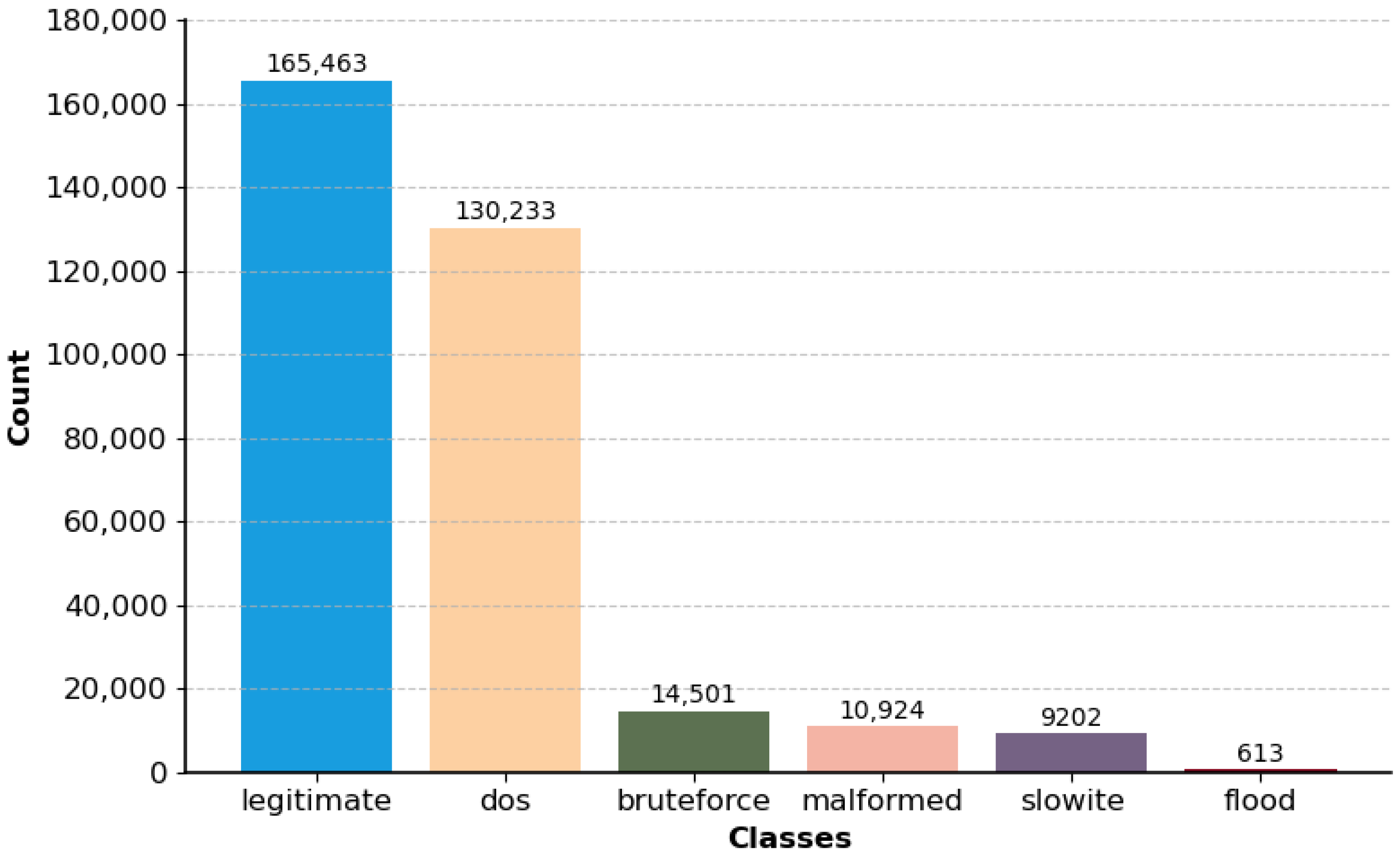
• Flooding Denial of Service (DoS): This attack targets the MQTT broker by establishing numerous connections and sending a high volume of messages using the MQTT-malaria tool (https://github.com/etactica/mqtt-malaria accessed on 13 March 2025), aiming to prevent the broker from serving legitimate clients.
• MQTT Publish Flood (flood): A single malicious device sends large amounts of MQTT data to exhaust server resources. This attack is implemented using the IoT-Flock tool.
• SlowITe (slowite): A slow DoS attack that initiates many connections to the MQTT broker with minimal bandwidth, using the MQTT service’s connection slots and causing a denial of service. This attack demonstrates efficiency in resource usage while achieving the attack’s objectives.
• Malformed Data (malformed): This attack sends malformed CONNECT or PUBLISH packets to the MQTT broker using the MQTTSA tool, aiming to trigger exceptions and disrupt normal operations.
• Brute Force Authentication (brute force): This attack attempts to crack MQTT user credentials using the MQTTSA tool and the rockyou.txt word list, simulating real-world brute force attacks to test the security of the MQTT authentication process.

To support different research needs, the authors in [23] organized the dataset into three formats: imbalanced data (which contain a significantly higher proportion of legitimate traffic compared to malicious traffic), balanced reduced data (where legitimate traffic was reduced to match the total volume of malicious traffic), and balanced augmented data (where attack traffic was augmented to balance with legitimate traffic).

In our study, we opted to use the balanced reduced data format. Our choice was guided by two primary considerations: (1) the need to mitigate the bias that often arises in imbalanced settings, where models tend to favor the majority class (legitimate traffic), potentially underperforming on minority (malicious) classes; and (2) the practical benefit of reduced computational cost and training time compared to the full 12 million entry imbalanced dataset. This format ensures that the total volume of legitimate traffic matches the sum of all malicious traffic instances, creating a 50:50 ratio between legitimate and malicious traffic. However, it is important to note that legitimate traffic remains the majority class when compared to individual attack types, as showcased in Figure 2, which aligns more closely with real-world scenarios where legitimate traffic dominates. This approach allows us to balance the dataset for effective model training while maintaining a realistic representation of class distributions. Additionally, the reduced dataset facilitates more straightforward computation as it contains fewer instances (330,936) compared to the imbalanced data (12,081,189) and the balanced augmented data (20 million). MQTTset ensures that our study is grounded in realistic and comprehensive data, reflecting real-world IoT network conditions and potential security threats.

3.2. Preprocessing and Exploratory Data Analysis

Preprocessing and exploratory data analysis (EDA) are critical steps in the machine learning workflow. Preprocessing involves preparing the raw data for analysis. This step includes handling missing values, converting data types, normalizing or standardizing data, and encoding categorical variables [24,25]. Preprocessing ensures that the dataset is consistent, complete, and formatted correctly for analysis. Effective preprocessing can significantly improve the performance of machine learning models by removing noise and irrelevant information. EDA involves analyzing datasets to summarize their main characteristics, often using visual methods. EDA helps to identify patterns, spot anomalies, and form hypotheses that can be further tested using more formal techniques [26].

In our study, we began with a review of the dataset to gather basic information, such as the number of entries and columns, with their respective data types. This initial overview confirmed that our dataset consists of 330,936 entries and 33 features, including numerical and categorical data types. Next, we verified the dataset for anomalies, including missing values and outliers. Subsequently, categorical features representing hexadecimal protocol-level values were directly converted to their numerical equivalents (decimal format) to preserve their inherent numeric semantics and ensure compatibility with machine learning algorithms. The target column consists of six traffic classes (legitimate, DoS, brute force, malformed, SlowITe, and flood), suitable for multiclass classification. For binary classification, we converted these into binary values: 0 for legitimate and 1 for attack classes. The data are balanced, with approximately 50% of the instances being attacks.

The initial statistics revealed that 12 features have constant values (zero mean and zero standard deviation). In other words, these features lack variability and provide no discriminatory power for predictive modeling. Additionally, we identified an outlier in one of the features, significantly distant from the rest of the dataset. Consequently, we dropped the 12 zero-variance features and removed the outlier to maintain data quality and interpretability. This reduced our feature set from 33 to 20.

3.3. Tools and Environment

This study was conducted using the Jupyter Notebook v6.4.8 within the Anaconda distribution. The main software tools and libraries used are listed in

Table 2. Utilized tools and libraries.

Tools/Software/Library	Version	Role
Anaconda	4.14.0	Package management and environment management
Jupyter Notebook	6.4.8	Interactive development environment
Python	3.9.12	Programming language
Pandas	1.4.4	For data manipulation and analysis
NumPy	1.22.4	For numerical operations
Scikit-Learn	1.0.2	For machine learning tasks including preprocessing, model training, and evaluation
Seaborn	0.11.2	For statistical data visualization
Matplotlib	3.5.1	For data visualization
TensorFlow	2.10.1	For building and training neural networks

to facilitate the reproducibility of the results. The computing environment comprises a machine with Intel64 Family 6 Genuine Intel, 36 cores processor, and a total memory of 64.0 GB. The system has two NVIDIA GeForce GTX 1080 Ti GPUs, NVIDIA-SMI Version 536.23 and CUDA Version 12.2. The complete codebase, covering preprocessing, feature selection, model training, and evaluation for both binary and multiclass classification tasks, is publicly available at the GitHub repository [27].

3.4. Feature Selection for Malicious Traffic Classification

FS is a critical step in the machine learning workflow that involves identifying and selecting a subset of relevant features for use in model development [28]. The primary goal of FS is to improve the model’s performance by removing irrelevant or redundant data, which can lead to overfitting and increased computational complexity [26]. This step is significant in high-dimensional data scenarios, where the number of features can be overwhelming, leading to the “curse of dimensionality” [17].

To address the need for efficient feature selection in our study, we introduce the SMDT method. SMDT leverages central moments (mean, standard deviation, skewness, and kurtosis) to identify the most significant features that distinguish legitimate from malicious traffic. These central moments were chosen for their complementary roles in capturing diverse statistical properties of the data: mean and standard deviation measure central tendency and variability, respectively, while skewness and kurtosis provide insights into the shape and extremities of the distribution [29]. These properties are particularly suited for the heterogeneous and often skewed distributions of IoT traffic data, where distinguishing benign and malicious patterns requires multidimensional statistical perspectives.

The diverse nature of IoT networks, with protocols like MQTT and varied attack patterns, often results in non-Gaussian data distributions; hence, IoT traffic’s complex and varied nature benefits significantly from such multidimensional statistical analysis. Unlike traditional feature selection methods, such as variance-based techniques that may overlook subtle but critical variations or correlation-based methods that primarily focus on linear relationships, SMDT identifies features with both linear and non-linear discriminatory power.

Hence, the SMDT method ensures the retention of only those features that exhibit significant divergence in their statistical moments between legitimate and malicious traffic. This is achieved through lightweight computations of central moments, which significantly reduce the feature set. As a result, the method simplifies ML models and enhances both training and testing times (and inference speeds during production), addressing the resource constraints typical of IoT devices. Additionally, the reduced computational overhead enables real-time processing capabilities, which are critical for ensuring IoT security.

As mentioned previously, in this study, we focus on the first four conventional statistical moments [30]: the first moment (the mean), the second central moment (the variance), and higher-order central moments such as skewness (the third moment) and kurtosis (the fourth moment). The SMDT approach involves a few steps. First, the dataset is split into separate subsets representing the legitimate and attack classes. For each subset (legitimate and attack classes), we calculate the statistical moments for each feature. As previously mentioned, these moments include the following:

-

The first moment, referred to as mean (µ), measures the central tendency that represents the average value of the feature. It is computed as follows:

$$\mu ={\displaystyle \frac{1}{n}}\sum _{i=1}^n{X}_i$$

(1)

where µ is the mean, Xi presents the feature’s value for the i-th instance, and n is the total number of instances.

-

The second central moment, referred to as variance (σ²), quantifies the extent to which each data point in the feature deviates from the mean, revealing the dispersion or variability in the feature values. Analysis of variance (ANOVA) is a widely utilized technique for data mining in various scientific and engineering disciplines [31]. However, in this study, we employed standard deviation, the square root of the variance, as it provides a more interpretable measure of dispersion [32]. The standard deviation (σ) is computed as follows:

$$\sigma =\sqrt{{\displaystyle \frac{1}{n}}\sum _{i=1}^n{(X_i-\mu )}^2}$$

(2)

-

The third central moment, skewness (γ₁), quantifies the asymmetry of a distribution. A skewness coefficient of zero signifies a perfectly symmetrical distribution. A positive skewness indicates that the distribution has a longer tail on the right side (right-skewed), whereas a negative skewness suggests a longer tail on the left side (left-skewed) [33,34]. However, skewness and kurtosis are interpreted differently across various studies and statistical software. As a result, different definitions and formulas can affect the interpretation of these measures. Therefore, our study uses the definitions and formulas provided by Python’s scientific statistics (SciPy. stats) module to ensure clarity. Precisely, skewness is calculated using the Fisher–Pearson coefficient, and kurtosis is measured as excess kurtosis, Fisher’s definition of kurtosis [33]. Hence, skewness is computed as follows:

$${\gamma }_1={\displaystyle \frac{1}{n}}\sum _{i=1}^n{\displaystyle \frac{{(X_i-\mu )}^3}{{\sigma }^3}}$$

(3)

-

The fourth central moment, kurtosis (γ₂), quantifies the “tailedness” of the distribution of the feature values. It indicates whether the data distribution has heavier tails (positive kurtosis) or lighter tails (negative kurtosis) compared to a normal distribution [35]. Kurtosis is computed as follows:   

$${\gamma }_2={\displaystyle \frac{1}{n}}\sum _{i=1}^n{\displaystyle \frac{{(X_i-\mu )}^4}{{\sigma }^4}}-3$$

(4)

As previously highlighted, if excess kurtosis (Fisher’s definition) [33] is utilized, the subtraction of 3 adjusts the kurtosis of a normal distribution to zero.

Once the statistical moments are computed, we proceed to calculate the absolute differences between the characteristics of the legitimate and the attack classes. This step involves determining the degree of deviation in the mean, standard deviation, skewness, and kurtosis of each feature between the two classes. For instance, the absolute difference in the mean is given by Equation (5), and similar formulas are applied for standard deviation, skewness, and kurtosis, respectively.

$${\Delta }_{u_i}=|{\mu }_{i,\mathrm{legitimate}}-u_{i,\mathrm{attack}}|$$

(5)

The absolute differences for each statistical moment are then summed for each feature to obtain a composite score representing the overall difference. A threshold value is then applied to the summed differences to identify the most significant features. Features with summed differences exceeding this threshold are considered and selected for model training. We iteratively adjust the threshold value to find the optimal threshold that leads to the best informative features. Using this approach, we reduced the number of features to 5. Algorithm 1 details the FS algorithm applied in this study, and

Table 3. Retained features.

No.	Name	Description	Protocol Layer
1	tcp.time_delta	Time TCP stream	TCP
2	tcp.len	TCP Segment Len	TCP
3	mqtt.kalive	Keep-Alive	MQTT
4	mqtt.msgid	Message Identifier	MQTT
5	mqtt.retain	Retain	MQTT

summarizes the retained features used for model training.

Algorithm 1: Feature Selection

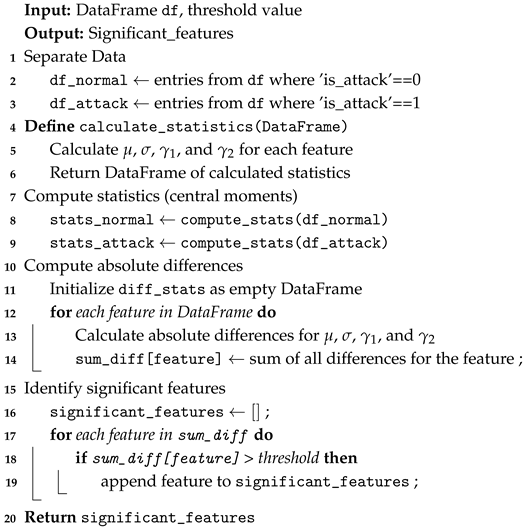
4. Experiment and Results

To validate the proposed SMDT method, we first applied it to select significant features for the binary classification of MQTT traffic. Subsequently, we extend our analysis to a multiclass classification approach to identify the specific class of attacks (brute force, DoS, flooding, malformed data, and slowite). The selected features were used to train and evaluate seven machine learning models, including traditional techniques, i.e., Random Forest (RF), Logistic Regression (LR), Decision Tree (DT), Gradient Boosting (GB), Extreme Gradient Boosting (XGBoost), and neural network-based models, i.e., Multilayer Perceptron (MLP) and Deep Neural Network (DNN), with a feedforward architecture.

4.1. Binary Classification

4.1.1. Model Training and Selection

In the case of binary classification, the goal is to identify whether the traffic is legitimate or an attack, without differentiating between specific attack types. As previously stated, we reorganized the data into two categories: legitimate (0) and attack (1). To effectively train models, we followed a standardized approach. We first separated the dataset into features and target variables. The features were scaled using a StandardScaler (Z-score normalization) to normalize the data, which is vital for many machine learning models to perform effectively [36,37].

Following the scaling process, the dataset was divided into training and testing sets, with 30% allocated for testing. A stratified split was used to preserve the class distribution of the target variable in both the training and testing sets. This stratified split helps preserve each class’s proportion, producing more balanced and representative subsets. Balanced and representative subsets enhance model performance and prevent bias in evaluation metrics [38].

To optimize the performance of the models, we employed grid search with cross-validation (GridSearchCV) [39] for hyperparameter tuning and cross-validating. Hyperparameters are settings that control how an ML model learns from data. Tuning involves systematically adjusting these settings (e.g., tree depth, learning rate) to find the combination that provides optimal performance. Thus, selecting appropriate values significantly impacts model performance [38]. For all employed learning algorithms except DNNs, we defined a parameter grid that specifies a range of values for each hyperparameter. Subsequently, GridSearchCV systematically explores multiple combinations of hyperparameter values to identify the optimal set of hyperparameters.

To mitigate the risk of overfitting, grid search is combined with cross-validation, a technique that divides the dataset into multiple subsets to train and test the model iteratively. In k-fold cross-validation, the training set is split into k equally sized, non-overlapping subsets. This approach creates multiple training–validation pairs for hyperparameter tuning and model selection, ensuring that the test set remains independent for the final evaluation of the model. For each iteration, k − 1 subsets are used for training, while the remaining subset is used to evaluate the model. This process is repeated k times, allowing each subset to be used as the validation set once. Consequently, different models and performance metrics are obtained for k. The final performance metric is calculated as the average of these k values. The choice of k often depends on the data size. However, 5 (utilized in this study) and 10 are the commonly used values of k in the literature [40]. After identifying the optimal hyperparameters and selecting the best model, we refit the model using the entire training set.

Table 4. Identified best hyperparameters (binary).

Algorithm	Identified Best Parameters (Based on the Defined Parameter Grid)
RF	bootstrap: True, criterion: gini, max_features: auto, min_samples_leaf: 1, min_samples_split: 2, n_estimators: 100
LR	fit_intercept: True, max_iter: 100, penalty: l2, solver: sag, tol: 0.0001
DT	criterion: gini, max_depth: 10, max_features: None, max_leaf_nodes: None, min_impurity_decrease: 0.0, min_samples_leaf: 5, min_samples_split: 2, splitter: best
GB	learning_rate: 0.1, max_depth: 5, min_samples_leaf: 1, min_samples_split: 10, n_estimators: 300
XGBoost	colsample_bytree: 0.8, gamma: 0, learning_rate: 0.1, max_depth: 5, n_estimators: 300, subsample: 0.8
MLP	activation: tanh, alpha: 0.0001, hidden_layer_sizes: (50, 50), learning_rate: constant, solver: adam

summarizes the optimized hyperparameters for each employed algorithm.

For DNN, we utilized Keras Tuner, a framework for hyperparameter optimization 41. Keras Tuner simplifies the process of defining search spaces with a define-by-run syntax and supports multiple search algorithms, including Bayesian Optimization, Hyperband, and Random Search [41,42,43]. Our study employed Random Search to explore a range of hyperparameters such as dropout and learning rates. The tuner was configured to perform five trials with three executions per trial, optimizing for validation accuracy.

To develop an optimal DNN model for our binary classification task, we utilized Keras with TensorFlow, leveraging the high-level API of Keras for building and training neural networks while benefiting from TensorFlow’s powerful backend capabilities [44]. The DNN architecture consisted of three hidden layers with 64, 32, and 16 neurons, respectively, each followed by a dropout layer to prevent overfitting [45]. Rectified Linear Unit (ReLU) [46,47] activation functions were used in the hidden layers, while a sigmoid [46] activation function was applied in the output layer to facilitate binary classification. We compiled the model using the Adaptive moment estimation (Adam) [48] optimizer with binary cross-entropy loss function [49]. After identifying the best hyperparameters through tuning, we retrained the model using the optimal settings. The training was conducted over ten epochs (the number of training iterations) with a validation split to monitor performance.

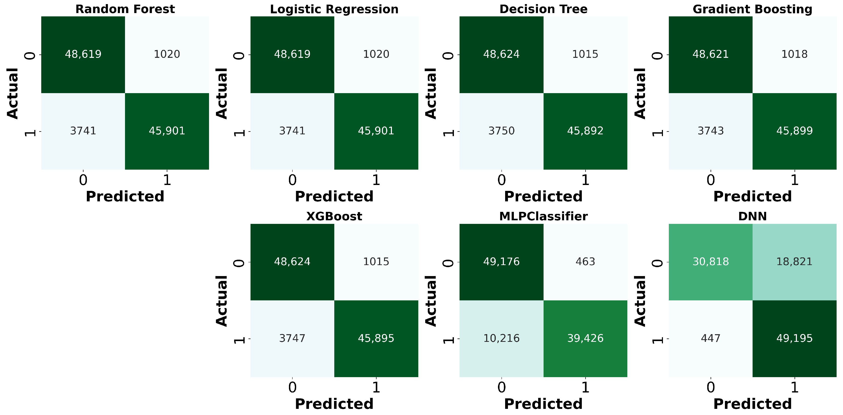
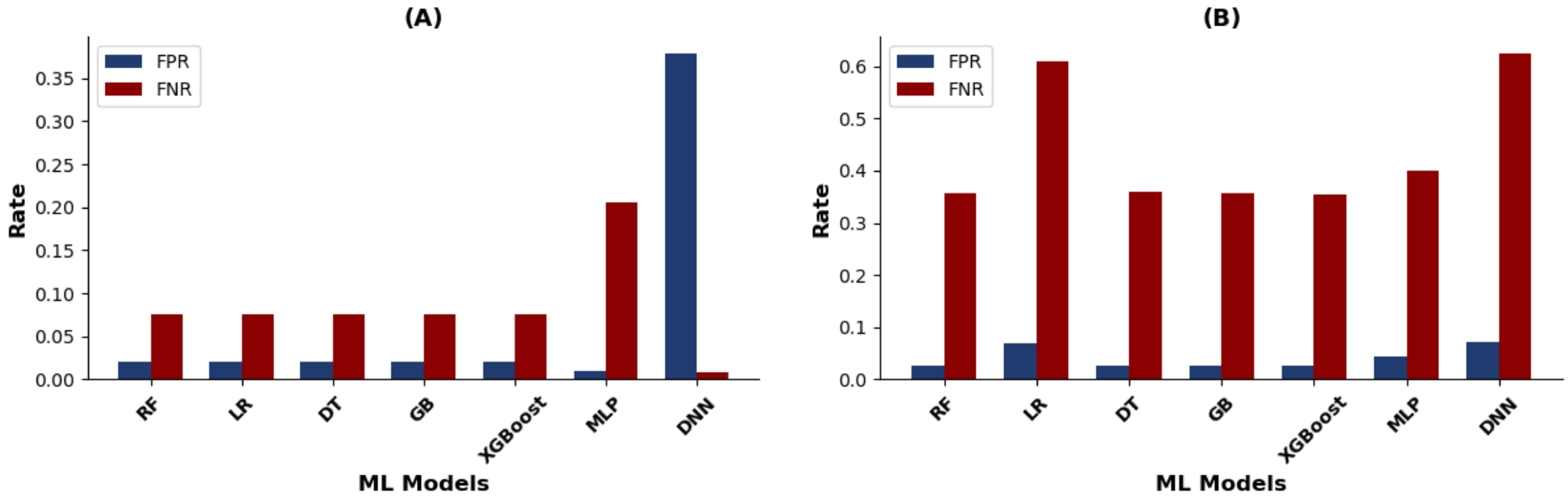
4.1.2. Performance Evaluation

We employed the commonly used performance metrics to evaluate the effectiveness of the selected ML models. These metrics include accuracy, precision, recall, F1-score, and ROC-AUC Score (Receiver Operating Characteristic Area Under the Curve) [50,51]. Additionally, to gain deeper insights into the model’s performance, we analyzed the confusion matrix, which provides a detailed breakdown of the model’s predictions. This allows us to understand the distribution of true positives (TPs), true negatives (TNs), false positives (FPs), and false negatives (FNs), as summarized in

Table 5. A binary classification confusion matrix [51].

Actual Traffic Class	Predicted as Attack	Predicted as Legitimate
Attack	TP	FN
Legitimate (Normal)	FP	TN

.

–

True Positive (TP): The model correctly predicts attack traffic.

–

False Negative (FN): The model incorrectly predicts attack traffic as legitimate traffic.

–

False Positive (FP): The model incorrectly predicts legitimate traffic as attack traffic.

–

True Negative (TN): The model correctly predicts legitimate traffic.

The confusion matrix also facilitates the computation of previously mentioned key performance metrics:

–

Accuracy measures the proportion of true results (both true positives and true negatives) among the total number of cases examined, computed as follows [50,52]:

$$\mathrm{Accuracy}={\displaystyle \frac{\mathrm{TP}+\mathrm{TN}}{\mathrm{TP}+\mathrm{TN}+\mathrm{FP}+\mathrm{FN}}}$$

(6)

–

Precision indicates the proportion of true positive results among all positive results (true positives and false positives). This is particularly important when the cost of false positives is high, such as incorrectly flagging legitimate traffic as an attack. It is computed as follows [50,52]:

$$\mathrm{Precision}={\displaystyle \frac{\mathrm{TP}}{\mathrm{TP}+\mathrm{FP}}}$$

(7)

–

Recall represents the proportion of true positive results among all actual positive instances (true positives and false negatives). This metric is significant when the cost of false negatives is high, such as missing an actual attack. It is computed as follows [50,52]:

$$\mathrm{Recall}={\displaystyle \frac{\mathrm{TP}}{\mathrm{TP}+\mathrm{FN}}}$$

(8)

–

F1-score represents the harmonic mean of precision (P) and recall (R), providing a single metric that balances both precision and recall [50]:

$$\mathrm{F}1 \mathrm{score}=2·{\displaystyle \frac{P·R}{P+R}}$$

(9)

–

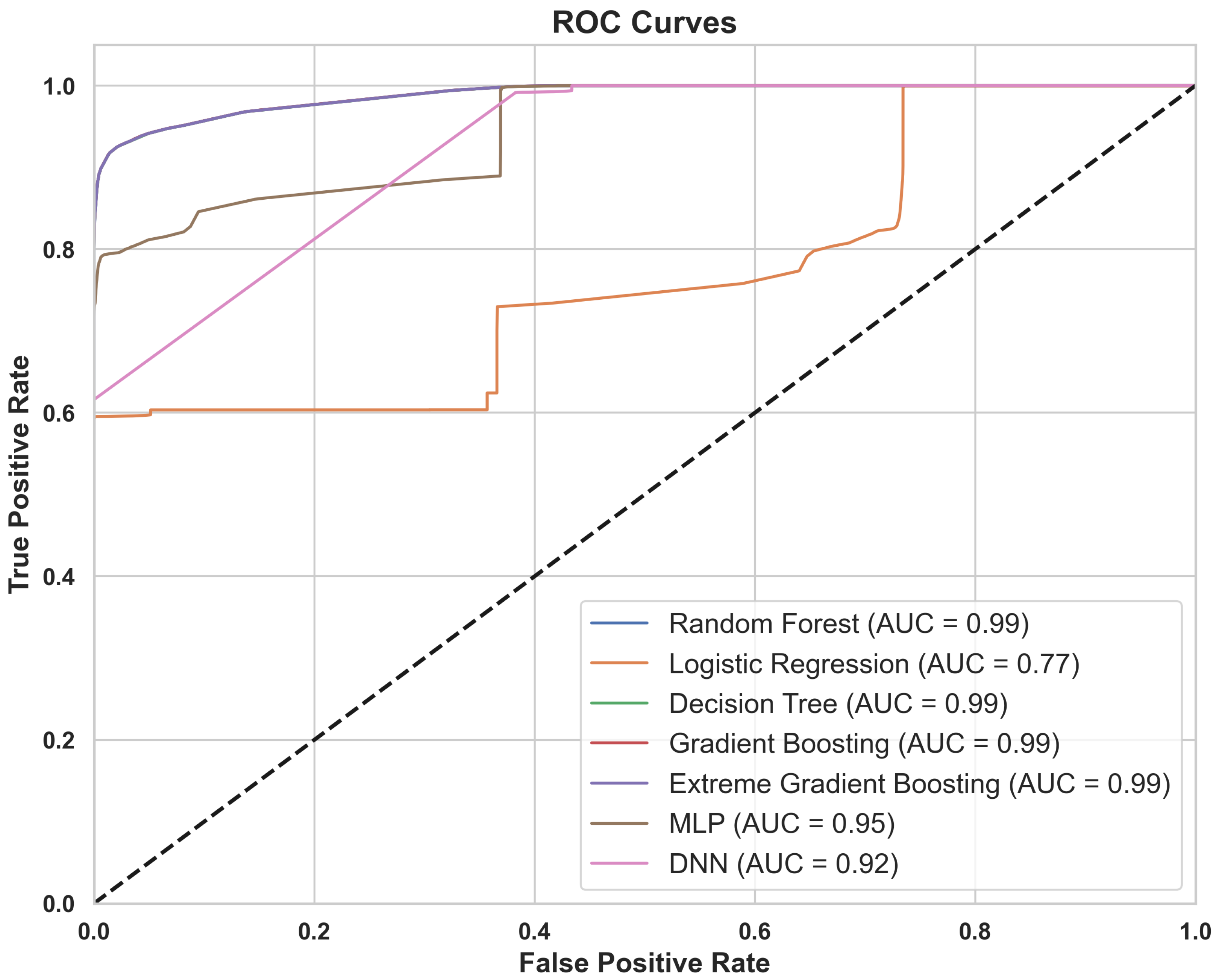
ROC-AUC score is a performance measurement for classification problems across various threshold settings [50]. The AUC score, which ranges from 0 to 1, quantifies the classifier’s ability to discriminate between positive (attack) and negative (legitimate) classes. A higher AUC value indicates better model performance. The ROC curve is created by plotting the true positive rate (TPR) against the false positive rate (FPR) at different threshold levels [51].

Table 6. Model evaluation: Performance metrics and computational times (binary).

Model	Accuracy	Precision	Recall	F1-Score	ROC-AUC	Searching Time (s)	Training Time (s)	Testing Time (s)
RF	0.95	0.95	0.95	0.95	0.99	2280.81	6.96	0.45
LR	0.95	0.95	0.95	0.95	0.99	221.58	11.27	0.99
DT	0.95	0.95	0.95	0.95	0.99	74.98	0.12	0.01
GB	0.95	0.95	0.95	0.95	0.99	3051.20	43.08	0.45
XGBoost	0.95	0.95	0.95	0.95	0.99	1252.83	12.38	0.04
MLP	0.89	0.91	0.89	0.89	0.95	3551.45	264.61	0.20
DNN	0.81	0.85	0.81	0.80	0.92	5602.99	722.57	6.44

summarizes the performance metrics obtained from the employed model. Searching Time (s) in Table 6, refers to the computational time required by hyperparameter optimization procedures (GridSearchCV for traditional ML models and Random Search via Keras Tuner for the DNN) to identify optimal hyperparameter combinations used for subsequent model training. Figure 3 showcases the confusion matrices for all models, and Figure 4 presents the ROC AUC scores.

4.2. Multiclass Classification

Following our initial experiments with binary classification to differentiate between legitimate and malicious traffic, we extended our analysis to a multiclass classification approach. This shift allowed us to evaluate how well the selected model can identify specific types of attacks, including brute force, DoS, flooding, malformed data, and SlowITe attacks. The significance of this extension is twofold. First, it provides a more granular understanding of the nature of the threats, enhancing the intrusion detection system’s capabilities. Second, it can help in developing more targeted mitigation strategies. Hence, we have six classes in this case, as opposed to the two in the binary classification scenario.

While most steps remained consistent with our binary classification approach, some adjustments were necessary for handling multiclass cases. In the multiclass classification approach, we initially used LabelEncoder to transform categorical labels into numerical values, making it easier to handle the labels computationally. Subsequently, we applied OneHotEncoder to the target variable. This encoding method converted the numerical labels into a binary matrix, facilitating the multiclass classification by ensuring that each class was represented correctly without implying any ordinal relationship. Moreover, as in the previous case, we employed GridSearchCV and Keras Tuner to optimize hyperparameters for our models. The identified best hyperparameters for the multiclass classification approach are summarized in

Table 7. Identified best hyperparameters (multiclass).

Algorithm	Identified Best Parameters (Based on the Defined Parameter Grid)
RF	bootstrap: True, max_depth: 20, min_samples_leaf: 2, min_samples_split: 5, n_estimators: 200
LR	C: 1.0, max_iter: 100, penalty: l2, solver: liblinear
DT	criterion: entropy, max_depth: 10, min_samples_leaf: 1, min_samples_split: 10, splitter: best
GB	learning_rate: 0.01, max_depth: 7, min_samples_leaf: 10, min_samples_split: 2, n_estimators: 300
XGBoost	colsample_bytree: 1.0, gamma: 0.1, learning_rate: 0.1, max_depth: 7, min_child_weight: 3, n_estimators: 100, subsample: 0.8
MLP	activation: tanh, alpha: 0.0001, hidden_layer_sizes: (100, 100), learning_rate: constant, solver: adam

.

To accommodate the multiclass nature of the problem, the DNN architecture was modified to include an output layer with nodes equal to the number of classes, using the softmax activation function [53]. The softmax function maps output values to a [0,1] range, allowing them to be interpreted as probabilities. As discussed in [35], the softmax function is essentially an extension of the sigmoid function [48] for multiclass classification, determining the probability of each class simultaneously [53,54]. Furthermore, we employed the Adam optimizer [48] with categorical_crossentropy loss, which is appropriate for multiclass classification tasks [49]. The performance metrics used in the binary classification case were adapted for the multiclass classification case. Therefore, the evaluation for multiclass classification included the following:

(a)

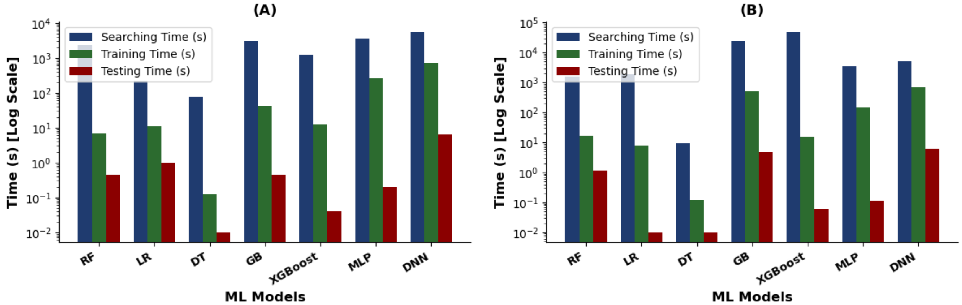
Classification report: This includes accuracy, precision, recall, and F1-score.

Table 8. Model performance: Evaluation metrics and computational times (mutliclass).

Model	Accuracy	Precision	Recall	F1-Score	Searching Time (s)	Training Time (s)	Testing Time (s)
RF	0.91	0.90	0.91	0.90	1547.43	16.21	1.15
LR	0.79	0.79	0.79	0.75	1834.67	8.00	0.01
DT	0.91	0.91	0.91	0.90	9.24	0.12	0.01
GB	0.91	0.91	0.91	0.90	24,489.46	505.96	4.80
XGBoost	0.91	0.91	0.91	0.90	49,323.92	15.75	0.06
MLP	0.82	0.85	0.82	0.80	3573.60	141.93	0.11
DNN	0.78	0.77	0.78	0.74	5081.92	702.20	6.03

summarizes the obtained results for these metrics. As previously defined, the “Searching Time (s)” reported in Table 8 refers to the computational time required by hyperparameter optimization procedures to identify the optimal hyperparameter combinations used for subsequent model training.

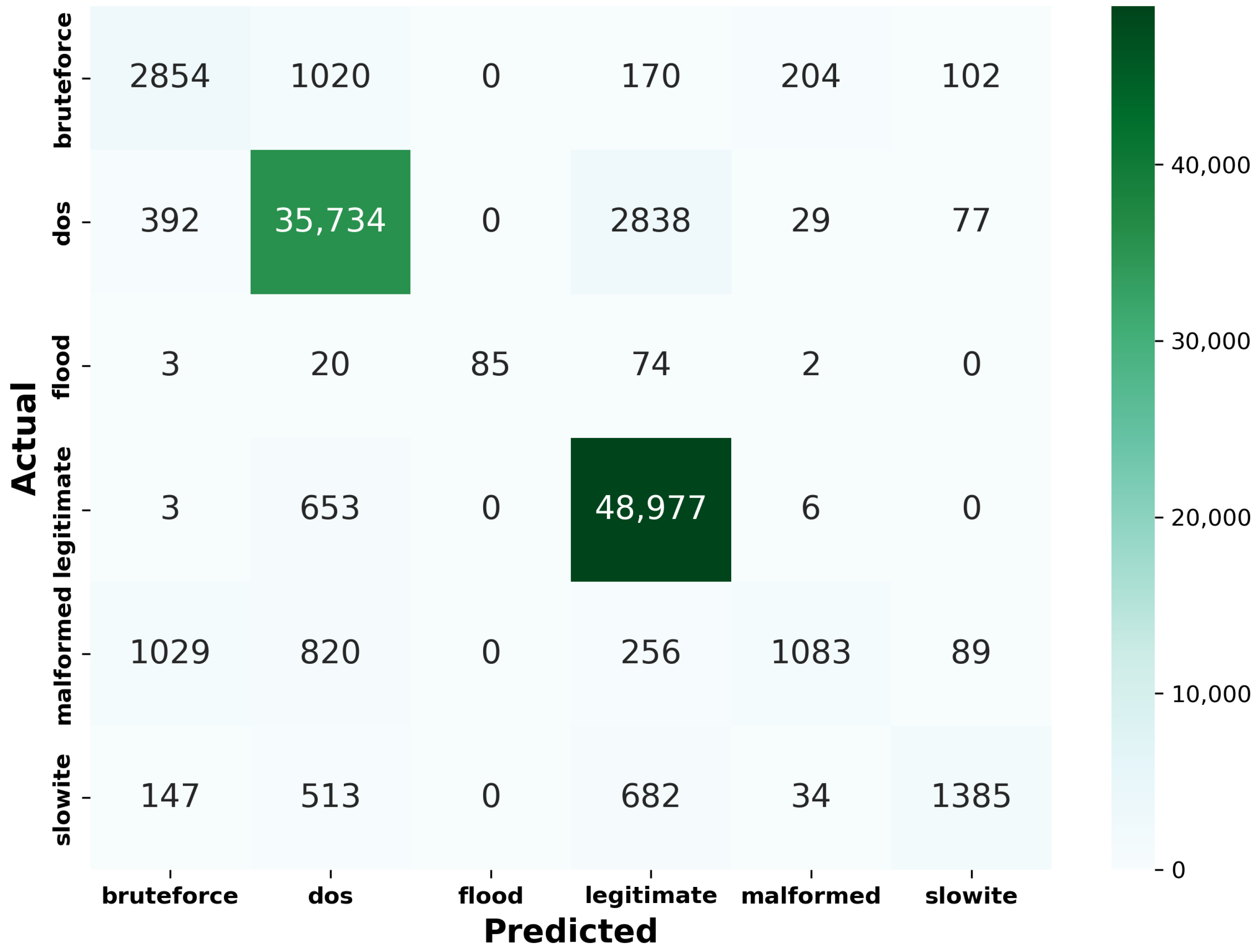
(b)

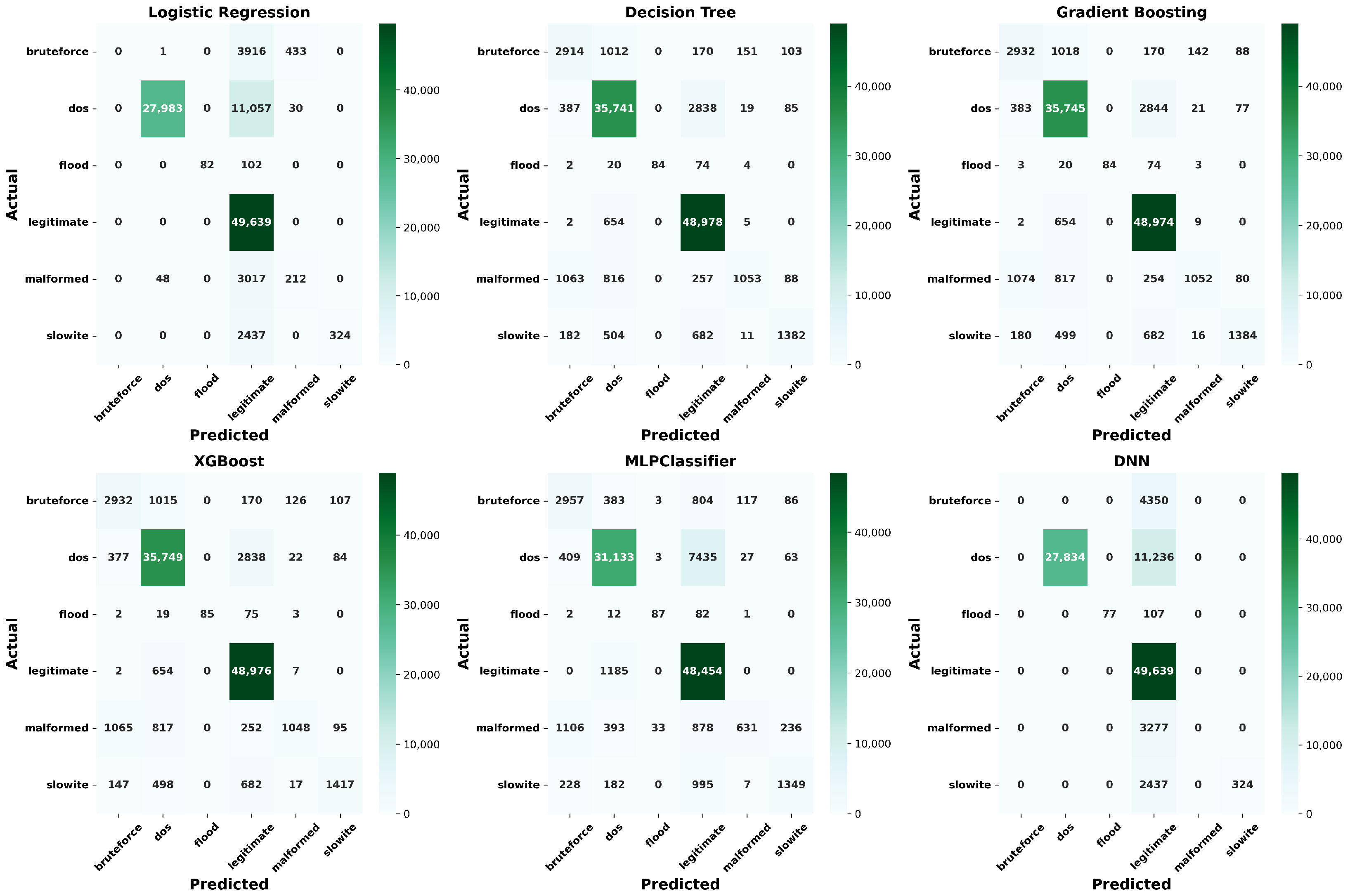
Confusion matrix: As previously discussed, the confusion matrix highlights the frequency of correct and incorrect predictions made by a model by comparing actual classifications to predicted classifications. Multiclass classification becomes more complex than binary classification. Instead of a simple 2 × 2 grid, the matrix expands to an N × N grid, where N represents the number of classes. Each cell in this grid represents the count of instances for each actual/predicted class pair, thus helping us to understand the model’s performance across all six classes, showing how many instances of each class are correctly or incorrectly predicted.

Table 9. Description of multiclass classification confusion matrix.

Actual/Predicted	Brute Force (B)	DoS (D)	Flood (F)	Legitimate (L)	Malformed (M)	SlowITe (S)
Brute Force (B)	TP (BB)	FP (BD)	FP (BF)	FN (BL)	FP (BM)	FP (BS)
DoS (D)	FP (DB)	TP (DD)	FP (DF)	FN (DL)	FP (DM)	FP (DS)
Flood (F)	FP (FB)	FP (FD)	TP (FF)	FN (FL)	FP (FM)	FP (FS)
Legitimate (L)	FP (LB)	FP (LD)	FP (LF)	TP (LL)	FP (LM)	FP (LS)
Malformed (M)	FP (MB)	FP (MD)	FP (MF)	FN (ML)	TP (MM)	FP (MS)
SlowITe (S)	FP (SB)	FP (SD)	FP (SF)	FN (SL)	FP (SM)	TP (SS)

is provided to facilitate the interpretation of the confusion matrix for each model, where the following definitions apply:

–

TP (XX): True positive for class X.

–

FP (XY): False positive, predicted as class Y but actual class is X.

–

FN (YX): False negative, actual class Y but predicted as class X.

For the sake of brevity, we present Figure 5, the confusion matrix for the RF model. The confusion matrices for the other six models are provided in the Appendix A (see Figure A1).

(c)

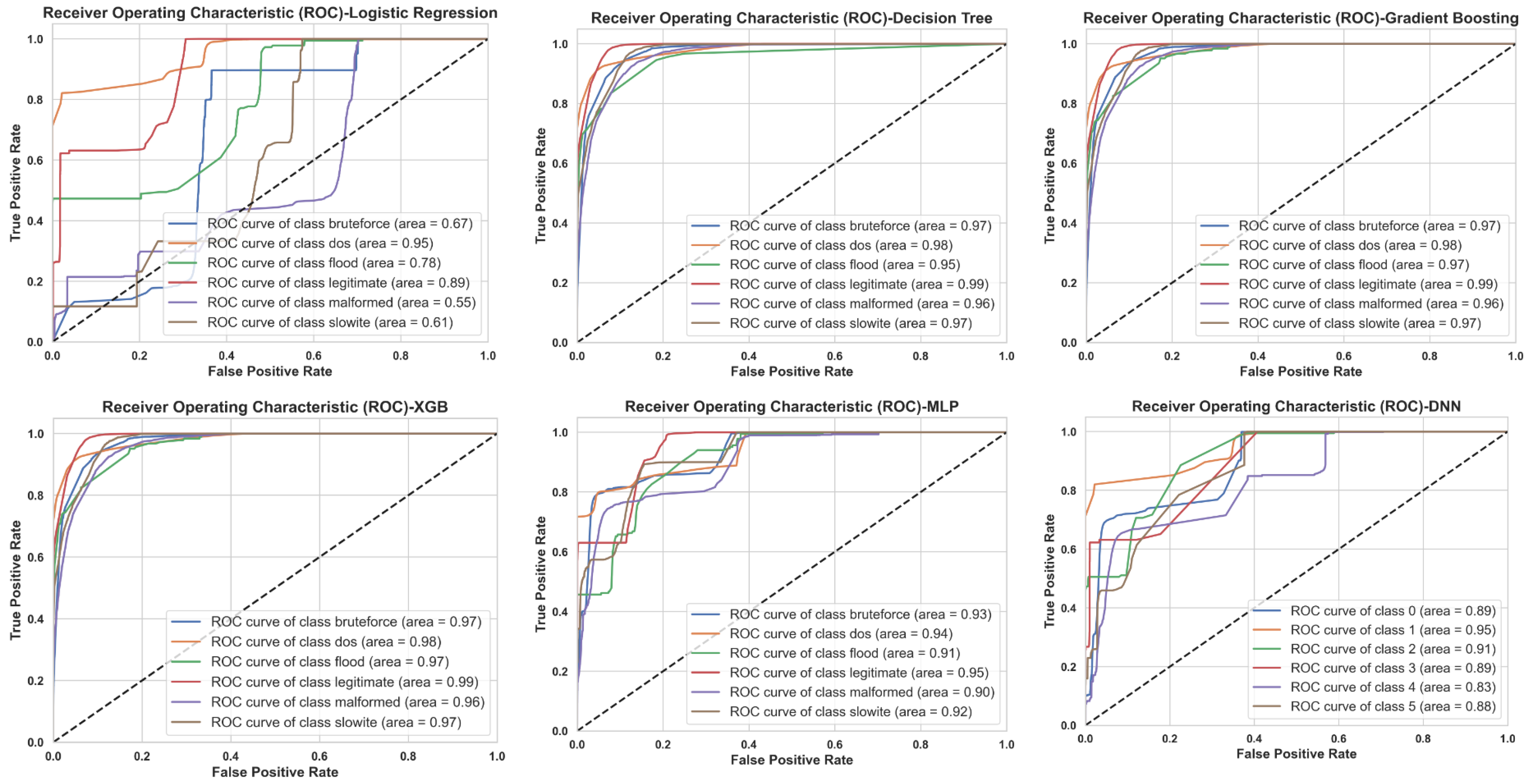
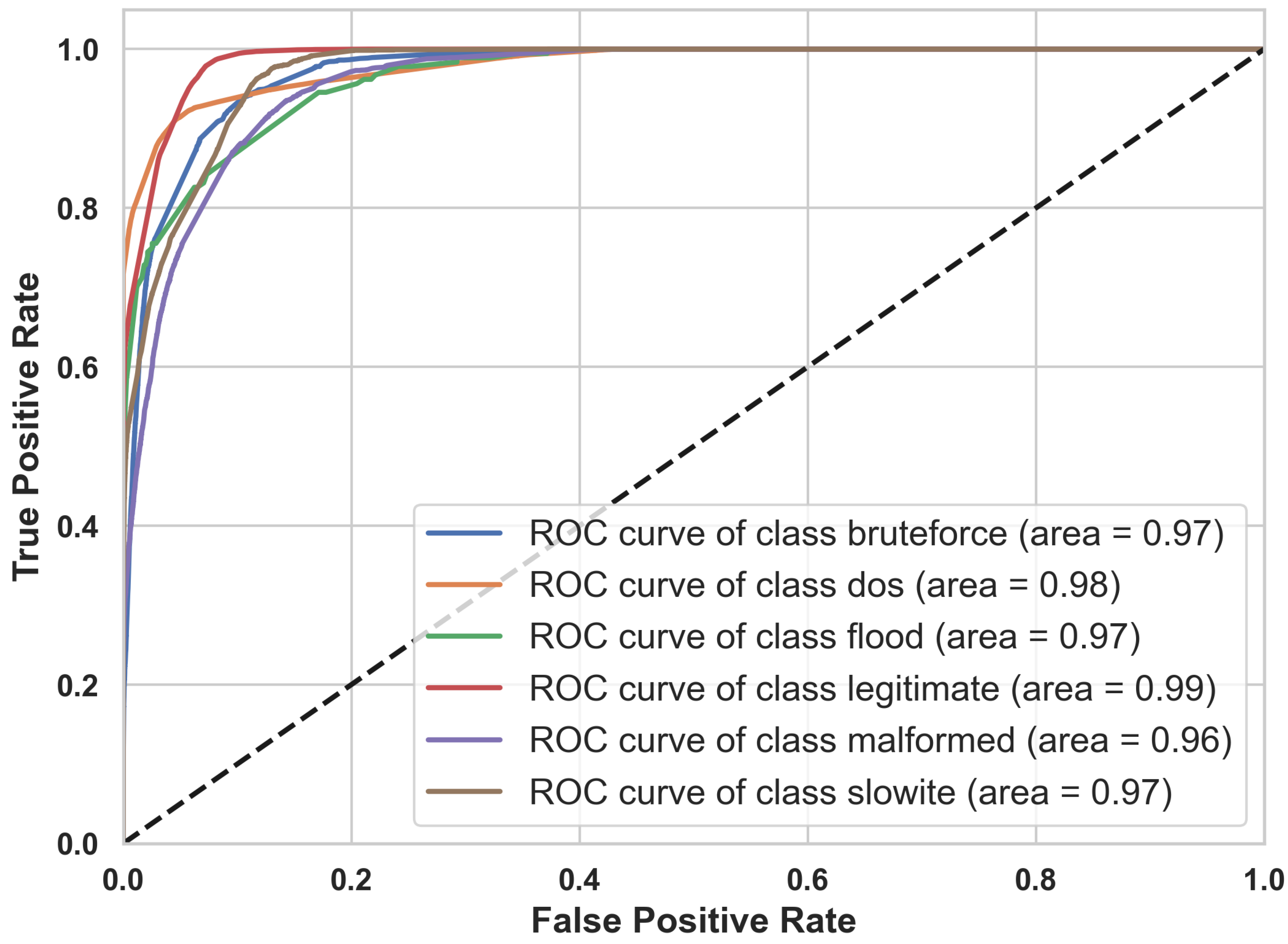
ROC-AUC: The approach used to compute ROC-AUC in the multiclass case differs from that in binary classification. A standard method in the literature is to produce one ROC curve for each class, treating each class as the positive class and all others as negative [51]. We computed the ROC-AUC using the One-vs.-Rest (OvR) approach for the multiclass classification. The AUC was evaluated and reported as a weighted average to account for class imbalances. For the sake of brevity, we present Figure 6, the ROC-AUC scores for the RF model. The ROC-AUC scores for the other six models are provided in the Appendix A (see Figure A2).

5. Discussion

In this section, we evaluate the proposed method’s performance. We compare the results obtained with those of the existing literature that uses the same dataset. Additionally, we analyze the performance of the employed models and discuss selecting the most suitable model.

5.1. Performance Analysis

For binary classification tasks, all models except the MLP and DNN performed exceptionally well with accuracy, precision, recall, and F1-score all around 0.95 and an ROC-AUC of 0.99. The MLP had a slightly lower performance with an accuracy of 0.89 and ROC-AUC of 0.95 (see Table 6). The DNN, however, had a significantly lower performance with an accuracy of 0.81 and an ROC-AUC of 0.92.

Nevertheless, the confusion matrices (see Figure 3) provided deeper insights. The DNN, despite its lower overall accuracy, achieved the highest number of true positives (49,195) and the fewest false negatives (447). However, it also exhibited a significantly high number of false positives (18,821), as reflected by its elevated FPR in Figure 7. This suggests that while the DNN is very sensitive (high recall), it lacks specificity, resulting in high false alarms. In real-time production environments, this behavior of the DNN may be undesirable as it leads to excessive false alarms and inefficient resource utilization. Conversely, the MLP had more false negatives (10,216) and fewer false positives (463). This indicates that the MLP missed more actual attacks (low recall) but generated fewer false alarms. This trade-off is critical in intrusion detection systems, where missing an attack (high FN) can cause more significant damage than having false alarms.

In the multiclass case, the class distribution was highly imbalanced, with legitimate traffic making up the majority and flooding attacks being the rarest. The performance metrics for the multiclass classification models are presented in Table 8. The RF, DT, GB, and XGBoost models achieved decent accuracy, precision, recall, and F1-scores around 0.90. LR and MLP classifier had lower performance, with accuracies of 0.79 and 0.82, respectively. The DNN again had the lowest performance, with an accuracy of 0.78.

The confusion matrices for multiclass classification (see Figure 5 and Figure A1) highlight that most misclassifications occurred in classes with fewer samples, such as malformed, SlowITe, and flooding. Hence, the models may benefit from further tuning or more sophisticated techniques to handle the rare classes effectively.

As depicted in Figure 8, the computational time varied significantly across models both in binary and multiclass cases (see also Table 6 and Table 8). DT, RF, and LR were the fastest. GB and XGBoost required slightly longer training times compared to the fastest models. MLP and DNN had the most extended training times, indicating potential issues with model complexity and computational efficiency, which might be a limitation for resource-constrained environments. We note that due to the wide variation in time measurements across different ML models, a logarithmic scale [55] was applied to the y-axis in Figure 8 to enhance the comparison of resource demands across models. A linear scale in this context would have made smaller values (testing times) nearly invisible and difficult to distinguish.

5.2. Comparative Analysis with Previous Studies Using MQTTset Dataset

In this section, we compare our results to prior studies that used different numbers of features from the same dataset, MQTTset.

Vaccari et al. [23] utilized 33 features and demonstrated that models like RF and DT achieved the highest accuracy of 91.59%. Notably, their study required substantial training times, highlighting a potential issue for real-time applications. Zeghida et al. [5] using 33 features showed improvements with ensemble methods such as stacking, which achieved an accuracy of 95.43% but at a high computational cost.

Al Hanif and Ilyas [4] reduced the feature set to 10 and showed that models like RF could achieve an accuracy of 96.33%. The training times were also relatively lower than those of Vaccari et al. [23] and Zeghida et al. [5]. However, it is essential to note that the training time may depend on the available computational resources, which can vary significantly across different studies.

Our study reduced the feature set from 33 to only 5 using SMDT. The selected five features still provide high performance with simpler models, as evidenced by the performance metrics. We achieved competitive accuracy rates with models such as RF, DT, GB, and XGBoost, reaching 95% in binary classification and 91% in multiclass classification. Without sacrificing performance, the significant reduction in feature dimensionality demonstrates SMDT’s potential for enhancing computational efficiency.

Table 10. Comparison of our study with previous works using MQTTset dataset.

Ref	Year	Features	Best Accuracy	Best F1-Score	Training Time (s)	Testing Time (s)
[23]	2020	33	(multiclass) RF, DT: 91.59%	RF, DT: 91.40%	2298.2762	125.8504
[5]	2023	33	(binary classes) Stacking: 95.42%	Stacking: 95.42%	250.05	0.94
[4]	2024	10	(binary classes) RF: 96.33%	RF: 96.32%	4.0888	0.1686
Our study	2025	5	(binary classes) RF, LR, DT, GB, XGBoost: 95% (multiclass) RF, DT, GB, XGBoost: 91%	(binary classes) RF, LR, DT, GB, XGBoost: 95% (multiclass) RF, DT, GB, XGBoost: 90%	(binary classes) 6.96, 11.27, 0.12, 43.08, 12.38 (multiclass) 16.21, 0.12, 505.96, 15.75	(binary classes) 0.45, 0.99, 0.01, 0.45, 0.04 (multiclass) 1.15, 0.01, 4.80, 0.06

summarizes this comparative analysis with previous studies.

5.3. Analysis and Selection of Models

The experimental results demonstrate the performance trade-offs among the various models evaluated in this study. Notably, DT and RF emerged as best performers for both binary and multiclass classification tasks with significantly low computational costs. DT, in particular, proved efficient with concise training (0.12 s) and testing times (0.01 s). The IoT environment processes continuous streams of real-time data. Real-time processing requires efficient algorithms to process data promptly and detect and respond to threats. Delayed detection (e.g., batch processing) may affect the security [56]. Hence, from this perspective, DT could be the best candidate for real-time/near-real-time intrusion detection in applications where fast detection and low energy consumption are critical.

Similarly, the ensemble techniques (GB and XGBoost) performed well but were more computationally expensive, thus suitable for scenarios where computational resources are not severely limited. While LR performed well in binary classification, it struggled more with the multiclass scenario, likely due to the complexity and imbalanced nature of the classes in the MQTTset. Its computational efficiency makes it a potential choice for time-sensitive applications, but its trade-off with accuracy in multiclass classification limits its effectiveness.

MLP and DNN underperformed compared to others, with the DNN having the lowest accuracy. Moreover, the computational cost of models like DNN may not be suitable for resource-constrained applications. For instance, the execution time of DT was reduced by approximately 99.98% compared to DNN, highlighting the importance of selecting less complex models in real-time scenarios. Similarly, RF offers a significant reduction in execution time, with a 97.37% reduction compared to MLP in the binary classification case, and an 88.58% reduction in the multiclass case, without sacrificing detection accuracy. This efficiency highlights the potential energy savings, as the reduced computational complexity scales directly with lower power consumption, which is especially beneficial in IoT environments.

Additionally, the importance of minimizing false negatives versus false positives should be considered based on the security priorities of the IoT network. As evidenced by the confusion matrices, different models offer varying trade-offs in the false positive/negative aspects. High false positives disrupt operations, while false negatives miss threats. Models with low FPR, such as RF and GB, are preferable in operational settings where false alarms can lead to unnecessary resource utilization. Conversely, models with high FNR, like DNN and LR, require further optimization to ensure comprehensive threat detection without sacrificing usability, particularly in multiclass scenarios where the risk of missed detections is higher.

However, selecting the appropriate model would depend on the application-specific requirements. Due to their efficiency, RF and DT could fit in scenarios with limited computational resources. In environments where computational power is less constrained, ensemble methods like GB and XGBoost could be more advantageous. On the other hand, the extended computational times of DNNs and MLP render them less practical for real-time processing but potentially valuable for offline analysis or environments with enough computational resources. Hence, it is important to strike a balance based on the specific use case, available resources, and acceptable performance-complexity trade-offs.

5.4. Limitations and Future Work

Although the proposed method effectively reduced the feature set while maintaining high detection accuracy, its applicability across other datasets and IoT protocols remains to be fully explored. The study leveraged the publicly available MQTTset dataset, which, although comprehensive and suitable for evaluating MQTT traffic, was generated in a simulated environment. Real-world IoT networks often feature additional complexities, such as dynamic traffic patterns, device heterogeneity, and environmental noise, which are not fully represented in the dataset. The selected features were optimal for the MQTTset dataset, but additional testing on datasets from other IoT ecosystems would help assess the scalability and adaptability of the approach to varying network conditions.

The employed dataset also focuses on a subset of common MQTT-related attacks, including doS, flood, brute force, slowITe, and malformed data attacks. While these represent critical vulnerabilities, they do not encompass more sophisticated threats such as advanced persistent threats (APTs). Expanding the scope to include a wider variety of attack scenarios in future research could improve the generalizability of the method to diverse IoT environments and emerging cybersecurity threats.

Furthermore, the computational efficiency observed in this study, particularly with lightweight models like DT and RF, was evaluated in a high-performance computing environment. While this demonstrates the suitability of the proposed method for resource-constrained devices, real-world testing on actual IoT hardware is necessary to validate its scalability and performance under live, large-scale deployment scenarios. Future work will focus on implementing the approach in real-time systems to evaluate its latency, throughput, and overall operational viability.

6. Conclusions

In this study, we demonstrated the effectiveness of SMDT as a practical feature selection method for identifying significant features, validated using the MQTTset dataset. Among the models evaluated, DT, RF, GB, and XGBoost emerged as top performers in both binary and multiclass classification, with DT standing out for its superior computational efficiency. This was evident as it outperformed more complex models like DNN, which, despite its sophisticated architecture, did not deliver proportional improvements in detection rates and instead highlighted the computational cost challenges, especially in IoT settings. These findings underline the trade-offs between model complexity, performance, and computational demand, suggesting that simpler and more efficient models could be more suitable for real-time applications in resource-limited IoT environments.

While the findings underline the importance of lightweight and efficient models for IoT applications, the study also identified areas for further research. Future work will address the limitations outlined, such as validating SMDT with real-world IoT datasets and expanding the range of attack types analyzed. Additionally, refining DNN architectures to improve efficiency and exploring cost-sensitive learning methods to mitigate class imbalance could further enhance model effectiveness.

References

1. Georgios, L.; Kerstin, S.; Theofylaktos, A. Internet of things in the context of industry 4.0: An overview. Int. J. Entrep. Knowl. 2019, 7, 4–19. [Google Scholar] [CrossRef]
2. Naik, N. Choice of effective messaging protocols for IoT systems: MQTT, CoAP, AMQP and HTTP. In Proceedings of the 2017 IEEE International Systems Engineering Symposium (ISSE), Vienna, Austria, 11–13 October 2017; pp. 1–7. [Google Scholar]
3. Al-Masri, E.; Kalyanam, K.R.; Batts, J.; Kim, J.; Singh, S.; Vo, T.; Yan, C. Investigating Messaging Protocols for the Internet of Things (IoT). IEEE Access 2020, 8, 94880–94911. [Google Scholar] [CrossRef]
4. Al Hanif, A.; Ilyas, M. Effective Feature Engineering Framework for Securing MQTT Protocol in IoT Environments. Sensors 2024, 24, 1782. [Google Scholar] [CrossRef] [PubMed]
5. Zeghida, H.; Boulaiche, M.; Chikh, R. Securing MQTT protocol for IoT environment using IDS based on ensemble learning. Int. J. Inf. Secur. 2023, 22, 1075–1086. [Google Scholar] [CrossRef]
6. Sadio, O.; Ngom, I.; Lishou, C. Lightweight Security Scheme for MQTT/MQTT-SN Protocol. In Proceedings of the 2019 Sixth International Conference on Internet of Things: Systems, Management and Security (IOTSMS), Granada, Spain, 22–25 October 2019; pp. 119–123. [Google Scholar]
7. Chen, F.; Huo, Y.; Zhu, J.; Fan, D. A Review on the Study on MQTT Security Challenge. In Proceedings of the 2020 IEEE International Conference on Smart Cloud (SmartCloud), Washington, DC, USA, 6–8 November 2020; pp. 128–133. [Google Scholar]
8. Lakshminarayana, S.; Praseed, A.; Thilagam, P.S. Securing the IoT Application Layer from an MQTT Protocol Perspective: Challenges and Research Prospects. IEEE Commun. Surv. Tutor. 2024, 26, 2510–2546. [Google Scholar] [CrossRef]
9. MQTT Organization. MQTT—The Standard for IoT Messaging. 2025. Available online: https://mqtt.org/ (accessed on 25 January 2025).
10. Bouzidi, M.; Gupta, N.; Cheikh, F.A.; Shalaginov, A.; Derawi, M. A Novel Architectural Framework on IoT Ecosystem, Security Aspects and Mechanisms: A Comprehensive Survey. IEEE Access 2022, 10, 101362–101384. [Google Scholar] [CrossRef]
11. HiveMQ. Securing MQTT Systems—MQTT Security Fundamentals. 2024. Available online: https://www.hivemq.com/blog/mqtt-security-fundamentals-securing-mqtt-systems/ (accessed on 26 January 2025).
12. ul A. Laghari, S.; Li, W.; Manickam, S.; Nanda, P.; Al-Ani, A.K.; Karuppayah, S. Securing MQTT Ecosystem: Exploring Vulnerabilities, Mitigations, and Future Trajectories. IEEE Access 2024, 12, 139273–139289. [Google Scholar]
13. Husnain, M.; Hayat, K.; Cambiaso, E.; Fayyaz, U.U.; Mongelli, M.; Akram, H.; Abbas, S.G.; Shah, G.A. Preventing MQTT Vulnerabilities Using IoT-Enabled Intrusion Detection System. Sensors 2022, 22, 567. [Google Scholar] [CrossRef]
14. Tuyishime, E.; Radu, F.; Cotfas, P.; Cotfas, D.; Balan, T.; Rekeraho, A. Online Laboratory Access Control with Zero Trust Approach: Twingate Use Case. In Proceedings of the 2024 16th International Conference on Electronics, Computers and Artificial Intelligence (ECAI), Iasi, Romania, 27–28 June 2024; IEEE: Piscataway, NJ, USA, 2024; pp. 1–7. [Google Scholar]
15. SANS Institute. Exposed Industrial Control System Remote Services: A Threat to Critical Infrastructure|SANS Webcast. 2023. Available online: https://www.sans.org/webcasts/exposed-industrial-control-system-remote-services-a-threat-to-critical-infrastructure/ (accessed on 13 January 2025).
16. Alaiz-Moreton, H.; Aveleira-Mata, J.; Ondicol-Garcia, J.; Muñoz-Castañeda, A.L.; García, I.; Benavides, C. Multiclass Classification Procedure for Detecting Attacks on MQTT-IoT Protocol. Complexity 2019, 2019, 6516253. [Google Scholar] [CrossRef]
17. Chen, R.C.; Dewi, C.; Huang, S.W.; Caraka, R.E. Selecting critical features for data classification based on machine learning methods. J. Big Data 2020, 7, 52. [Google Scholar] [CrossRef]
18. Kornaros, G. Hardware-Assisted Machine Learning in Resource-Constrained IoT Environments for Security: Review and Future Prospective. IEEE Access 2022, 10, 58603–58622. [Google Scholar] [CrossRef]
19. Fatima, M.; Rehman, O.; Ali, S.; Niazi, M.F. ELIDS: Ensemble Feature Selection for Lightweight IDS against DDoS Attacks in Resource-Constrained IoT Environment. Future Gener. Comput. Syst. 2024, 159, 172–187. [Google Scholar] [CrossRef]
20. CNR IEIIT. MQTTset. 2021. Available online: https://www.kaggle.com/datasets/cnrieiit/mqttset (accessed on 5 January 2025).
21. Al-Fayoumi, M.; Abu Al-Haija, Q. Capturing low-rate DDoS attack based on MQTT protocol in software Defined-IoT environment. Array 2023, 19, 100316. [Google Scholar] [CrossRef]
22. Hindy, H.; Bayne, E.; Bures, M.; Atkinson, R.; Tachtatzis, C.; Bellekens, X. Machine Learning Based IoT Intrusion Detection System: An MQTT Case Study (MQTT-IoT-IDS2020 Dataset). arXiv 2020, arXiv:2006.15340. [Google Scholar]
23. Vaccari, I.; Chiola, G.; Aiello, M.; Mongelli, M.; Cambiaso, E. MQTTset, a New Dataset for Machine Learning Techniques on MQTT. Sensors 2020, 20, 6578. [Google Scholar] [CrossRef]
24. Ramasubramanian, K.; Singh, A. Data Preparation and Exploration. In Machine Learning Using R: With Time Series and Industry-Based Use Cases in R; Ramasubramanian, K., Singh, A., Eds.; Apress: Berkeley, CA, USA, 2019; pp. 35–77. [Google Scholar]
25. Wongsuphasawat, K.; Liu, Y.; Heer, J. Goals, Process, and Challenges of Exploratory Data Analysis: An Interview Study. arXiv 2019, arXiv:1911.00568. [Google Scholar]
26. García, S.; Ramírez-Gallego, S.; Luengo, J.; Benítez, J.M.; Herrera, F. Big data preprocessing: Methods and prospects. Big Data Anal. 2016, 1, 9. [Google Scholar] [CrossRef]
27. Tuyishime, E. Traffic Classification for MQTT IoT Network-Based Security Attacks. 2025. Available online: https://github.com/emmanuel-tuyishime/Traffic-Classification-for-MQTT-IoT-Network-Based-Security-Attacks- (accessed on 4 April 2025).
28. Chandrashekar, G.; Sahin, F. A survey on feature selection methods. Comput. Electr. Eng. 2014, 40, 16–28. [Google Scholar] [CrossRef]
29. Li, T. Robust estimations from distribution structures: II. Central Moments. arXiv 2024, arXiv:2403.14570. [Google Scholar] [CrossRef]
30. Ulrych, T.J.; Velis, D.R.; Woodbury, A.D.; Sacchi, M.D. L-moments and C-moments. Stoch. Environ. Res. Risk Assess. 2000, 14, 50–68. [Google Scholar] [CrossRef]
31. Kaufmann, J.; Schering, A. Analysis of Variance ANOVA. In Wiley Encyclopedia of Clinical Trials; John Wiley & Sons, Ltd.: Hoboken, NJ, USA, 2007. [Google Scholar]
32. Ivie, J.; MacKay, A. Measures of Variability; Tulsa Community College: Tulsa, OK, USA, 2021. [Google Scholar]
33. Zwillinger, D.; Kokoska, S. CRC Standard Probability and Statistics Tables and Formulae; CRC Press: Boca Raton, FL, USA, 1999. [Google Scholar]
34. Guo, Y.; Kibria, B.G. On Some Statistics for Testing the Skewness in a Population: An Empirical Study. Appl. Appl. Math. Int. J. AAM 2017, 12, 6. [Google Scholar]
35. Yusoff, S.b.; Bee Wah, Y. Comparison of conventional measures of skewness and kurtosis for small sample size. In Proceedings of the 2012 International Conference on Statistics in Science, Business and Engineering (ICSSBE), Langkawi, Malaysia, 10–12 September 2012; pp. 1–6. [Google Scholar]
36. Raju, V.N.G.; Lakshmi, K.P.; Jain, V.M.; Kalidindi, A.; Padma, V. Study the Influence of Normalization/Transformation process on the Accuracy of Supervised Classification. In Proceedings of the 2020 Third International Conference on Smart Systems and Inventive Technology (ICSSIT), Tirunelveli, India, 20–22 August 2020; pp. 729–735. [Google Scholar]
37. Singh, D.; Singh, B. Investigating the impact of data normalization on classification performance. Appl. Soft Comput. 2020, 97, 105524. [Google Scholar] [CrossRef]
38. Raschka, S. Model Evaluation, Model Selection, and Algorithm Selection in Machine Learning. arXiv 2020, arXiv:1811.12808. [Google Scholar]
39. GridSearchCV. 2024. Available online: https://scikit-learn.org/stable/modules/generated/sklearn.model_selection.GridSearchCV.html (accessed on 9 January 2025).
40. Stapor, K.; Ksieniewicz, P.; García, S.; Woźniak, M. How to design the fair experimental classifier evaluation. Appl. Soft Comput. 2021, 104, 107219. [Google Scholar] [CrossRef]
41. O’Malley, T.; Bursztein, E.; Long, J.; Chollet, F.; Jin, H.; Invernizzi, L. KerasTuner. 2019. Available online: https://github.com/keras-team/keras-tuner (accessed on 9 April 2025).
42. Joshi, S.; Owens, J.A.; Shah, S.; Munasinghe, T. Analysis of Preprocessing Techniques, Keras Tuner, and Transfer Learning on Cloud Street image data. In Proceedings of the 2021 IEEE International Conference on Big Data (Big Data), Orlando, FL, USA, 15–18 December 2021; pp. 4165–4168. [Google Scholar]
43. Shawki, N.; Nunez, R.R.; Obeid, I.; Picone, J. On Automating Hyperparameter Optimization for Deep Learning Applications. In Proceedings of the 2021 IEEE Signal Processing in Medicine and Biology Symposium (SPMB), Philadelphia, PA, USA, 4 December 2021; pp. 1–7. [Google Scholar]
44. Joseph, F.J.J.; Nonsiri, S.; Monsakul, A. Keras and TensorFlow: A Hands-On Experience. In Advanced Deep Learning for Engineers and Scientists: A Practical Approach; Prakash, K.B., Kannan, R., Alexander, S.A., Kanagachidambaresan, G.R., Eds.; Springer International Publishing: Cham, Switzerland, 2021; pp. 85–111. [Google Scholar]
45. Srivastava, N.; Hinton, G.; Krizhevsky, A.; Sutskever, I.; Salakhutdinov, R. Dropout: A Simple Way to Prevent Neural Networks from Overfitting. J. Mach. Learn. Res. 2014, 15, 1929–1958. [Google Scholar]
46. Hara, K.; Saito, D.; Shouno, H. Analysis of function of rectified linear unit used in deep learning. In Proceedings of the 2015 International Joint Conference on Neural Networks (IJCNN), Killarney, Ireland, 12–17 July 2015; pp. 1–8. [Google Scholar]
47. Agarap, A.F. Deep Learning using Rectified Linear Units (ReLU). arXiv 2019, arXiv:1803.08375. [Google Scholar]
48. Kingma, D.P.; Ba, J. Adam: A Method for Stochastic Optimization. arXiv 2017, arXiv:1412.6980. [Google Scholar]
49. Ho, Y.; Wookey, S. The Real-World-Weight Cross-Entropy Loss Function: Modeling the Costs of Mislabeling. IEEE Access 2020, 8, 4806–4813. [Google Scholar] [CrossRef]
50. Raschka, S. An Overview of General Performance Metrics of Binary Classifier Systems. arXiv 2014, arXiv:1410.5330. [Google Scholar]
51. Tharwat, A. Classification assessment methods. Appl. Comput. Inform. 2020, 17, 168–192. [Google Scholar] [CrossRef]
52. Goli, Y.D.; Ambika, R. Network Traffic Classification Techniques—A Review. In Proceedings of the 2018 International Conference on Computational Techniques, Electronics and Mechanical Systems (CTEMS), Belgaum, India, 21–22 December 2018; pp. 219–222. [Google Scholar]
53. Sharma, S.; Sharma, S.; Athaiya, A. Activation functions in neural networks. Int. J. Eng. Appl. Sci. Technol. 2020, 4, 310–316. [Google Scholar] [CrossRef]
54. Mercioni, M.A.; Holban, S. The Most Used Activation Functions: Classic Versus Current. In Proceedings of the 2020 International Conference on Development and Application Systems (DAS), Suceava, Romania, 21–23 May 2020; pp. 141–145. [Google Scholar]
55. Höhn, M.; Wunderlich, M.; Ballweg, K.; von Landesberger, T. Width-Scale Bar Charts for Data with Large Value Range. In Proceedings of the EuroVis (Short Papers), Norrköping, Sweden, 25–29 May 2020; pp. 103–107. [Google Scholar]
56. Alsoufi, M.A.; Razak, S.; Siraj, M.M.; Nafea, I.; Ghaleb, F.A.; Saeed, F.; Nasser, M. Anomaly-Based Intrusion Detection Systems in IoT Using Deep Learning: A Systematic Literature Review. Appl. Sci. 2021, 11, 8383. [Google Scholar] [CrossRef]
Figure 1. Overall implementation framework.
Applsci 15 04252 g001
Figure 2. Traffic distribution.
Applsci 15 04252 g002
Figure 3. Confusion matrix for all employed models (binary).
Applsci 15 04252 g003
Figure 4. ROC-AUC scores for all employed models (binary).
Applsci 15 04252 g004
Figure 5. Confusion matrix–Random Forest.
Applsci 15 04252 g005
Figure 6. ROC-AUC score–Random Forest.
Applsci 15 04252 g006
Figure 7. FPR and FNR across ML models: (A) Binary classification case and (B) multiclass classification case.
Applsci 15 04252 g007
Figure 8. Computational time across ML models: (A) Binary classification case and (B) multiclass classification case.
Applsci 15 04252 g008