
Design and Development of Interactive Software Models for Teaching Coding Theory: A Case Study on Hamming Codes—General Algorithm


Abstract
1. Introduction
- Real-time feedback—students receive automated guidance and analysis of their errors during task completion.
- Gamification through a point system and individual tasks—engaging students by dynamically assigning exercises with progressive difficulty.
- Process visualization—presenting the computational steps in encoding and/or decoding, which supports understanding abstract concepts.
2. Materials and Methods
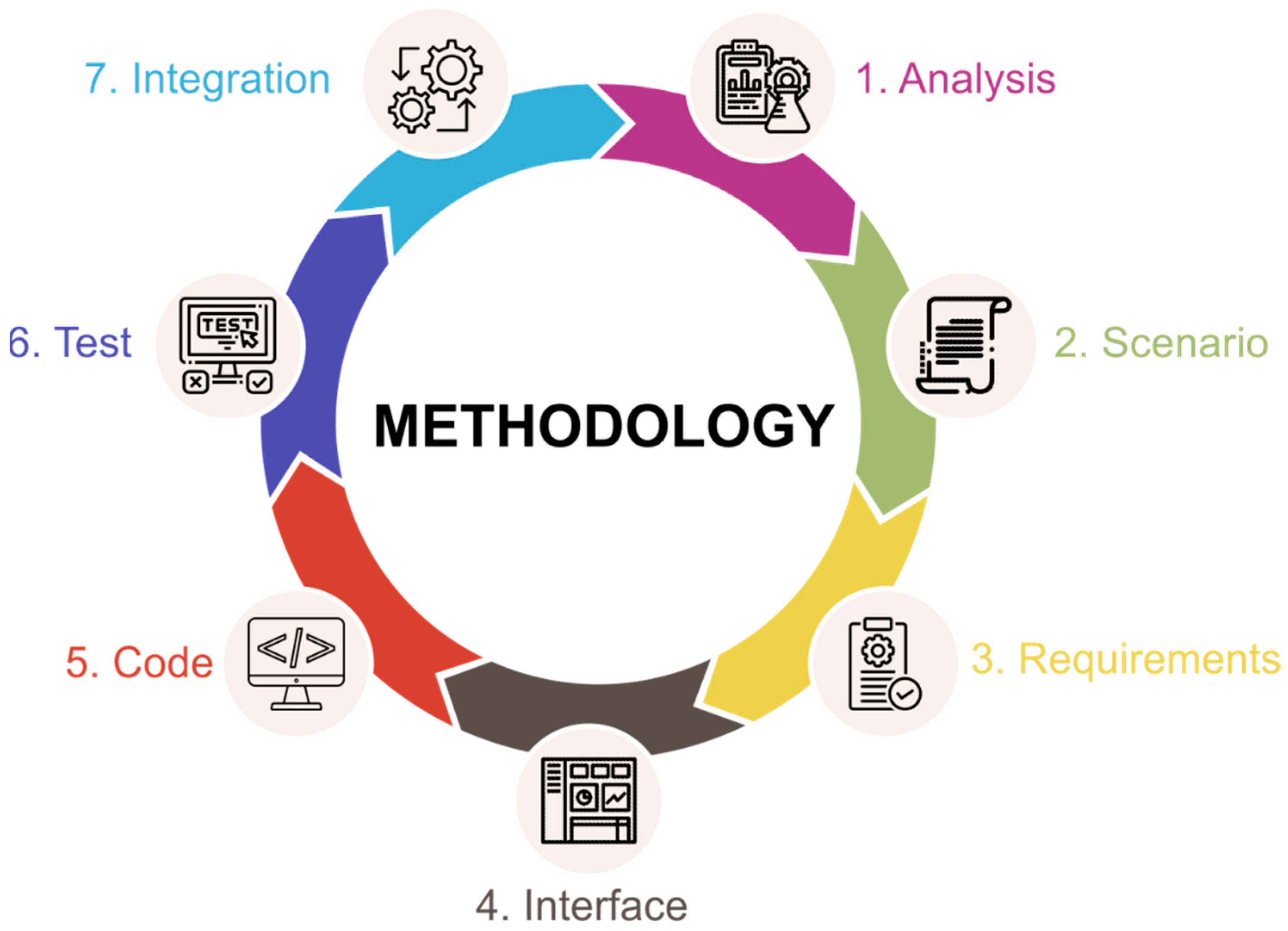
2.1. A Methodology for Designing and Developing an Interactive Software Model for Solving Tasks in the Field of Coding Theory
- (1)
- Analysis. During this first stage, detailed analysis is required on the theoretical aspects relating to the Hamming codes. Therefore, it entails:
- -
- A detailed analysis of the theoretical foundations of the functioning of Hamming codes, including the error-detection and correction approach that this code implements.
- -
- A deep summary of the mathematical computations and logical constructs inherent in the code, including the mechanisms for calculating check bits and identifying the locations of errors.
- -
- An understanding of the Hamming code’s constraints and capabilities is necessary to determine what the tool should include to provide the best possible training on the subject.
- (2)
- Scenario. After the analysis process, a scenario is created to solve problems using the Hamming code. A scenario is an overall structure or a guide that includes the following steps:
- -
- Description of tasks that users need to be able to perform with the tool. For example, detecting errors in a message or correcting any errors identified.
- -
- Defining the sequence of steps that will lead users through the process of solving problems with the Hamming code. It could include instructions for calculating check bits, error detection, and presentation of the result.
- -
- Creating interactive elements and tasks that will enable a user to put theoretical knowledge into practice. For example, interactive questions, filling in tables, and process visualizations.
- -
- Outlining the approach to the feedback system that the tool will implement, to help students understand and correct their solutions.
- (3)
- Requirements. At this stage, the functional and non-functional requirements of the tool are defined. These requirements will serve as a basis for all the other steps in the process of development:
- -
- Functional requirements: they describe the specific functions and abilities that the tool should be able to perform, such as:
- -
- Providing interactive exercises for use with Hamming codes;
- -
- The ability to enter values and see related results;
- -
- A system that randomly injects errors into code combinations that the user must find and correct.
- -
- Non-functional requirements: these specifications refer to attributes related to the quality and performance of the software, such as:
- -
- Processing speed—the tool must work quickly and efficiently;
- -
- Intuitiveness and ease of use—the interface must be easy to use;
- -
- Compatibility with different platforms—the tool must be accessible from different devices and browsers;
- -
- Reliability and security—the data and results entered by the user must be protected.
- (4)
- Interface. At this stage of the methodology, a prototype of the user interface (UI) is created to determine the appearance (view) of the software from the user’s perspective:
- -
- Design of the main view, in which the processes of coding, error detection, and correction will be visualized;
- -
- Navigation and accessibility—the structure of the interface should be simple and easy to understand so that users can be orientated quickly and start working;
- -
- Interactive elements, such as data entry fields, buttons for starting simulations, data visualizations, and feedback on correct or incorrect decisions;
- -
- Color scheme and design elements that make the interface attractive and intuitive, without unnecessary complexity, especially for younger users or beginners in the field.
- (5)
- Code. At this stage, the program code of the software tool is compiled:
- -
- Selection of a programming language and technologies (e.g., PHP, JavaScript, HTML/CSS, if it is a web-based application), tailored to the needs of the software and technical requirements;
- -
- Implementation of the basic algorithms necessary for working with the Hamming code—calculating the check bits, detecting errors, correcting them, and providing the result;
- -
- Development of user interaction modules, such as visualizing the error-correction process and providing data entry capabilities;
- -
- Integration of the algorithms and logic with the user interface to ensure smooth and functional interaction.
- (6)
- Test. Testing is a critical stage that ensures the quality and reliability of the software:
- -
- Functional testing—checking that all the functionalities set out in the requirements work correctly. This includes:
- -
- Checking the algorithms for encoding and decoding, and whether they successfully detect and correct errors;
- -
- User interface tests for interactivity and ease of use;
- -
- Error testing and debugging—identifying and fixing errors in the code that can cause crashes or incorrect operation of the software;
- -
- Performance and security tests—measuring the execution time of basic operations and ensuring the security of user data.
- (7)
- Integration. The final stage is the integration of the software tool into a common virtual laboratory:
- -
- Integrating the tool with other educational software in the laboratory, if any, which may include a common user interface or database;
- -
- Creating easy access to the tool for users, for example through a centralized platform or web portal;
- -
- Testing the integration in a real learning environment to ensure that all components work together properly and interact seamlessly;
- -
- Post-integration support and monitoring to ensure that the tool continues to work properly in real-world conditions and is updated as needed.
2.2. Designing an Interactive Software Model for Solving Problems with the “Hamming Code—General Method”
2.2.1. General Concepts of Error Control Codes
- Error control codes, also known as channel (noise-tolerant) codes, serve to detect and correct (or only detect) any errors received during data transmission or storage at the expense of adding information redundancy to the data [23]. Channel codes can be error-detecting-only codes or error-detecting and error-correcting codes. On the other hand, they are divided into block and convolutional (continuous) codes. Block codes are those in which each character of a given message corresponds to a precisely defined code combination. They are divided into separable (when it is known which bits in the code combination are information and which are control) and inseparable (all bits are both information and control) [24].
- In the theory of channel coding, the following concepts are defined [24]:
- Information combination (IC)—these are the information bits that will be coded, and the number of bits in one IC will conventionally be denoted by .
- Control bits ()—these are the bits that are added to the information bits and thus form the code combination. The number of control bits will conventionally be denoted by .
- Code combination (CC) or code word —this is the coded combination, including the information and control bits. The number of bits in one code combination (CC) will conventionally be denoted by , as:
- Multiplicity of errors ()—number of erroneous bits in one code combination.
- Code (Hamming) distance between two combinations ()—number of bits by which the two combinations differ. For codes without redundancy, it is characteristic that , and for codes with redundancy—.
- Minimum code distance of the code ()—the smallest possible code distance between two code combinations of a given code.
- Information redundancy—extra (check) bits added to the information, with the help of which it is checked whether errors occurred during the transmission/storage of the message.
- Transmission rate of the code combination ():where:—number of information bits in the code combination;—total number of bits in the code combination.
- Weight of the code combination in binary coding—number of ones (1s) in the code word.
- Correction capability ()—the correction capability of a given code is the number of errors that the code can correct and is closely related to the minimum code distance with the following dependence [20]:where denotes the largest integer not exceeding the value of .
- Detectability ()—the detectability of a given code is the number of errors it can detect and has the following relationship with :
2.2.2. Analysis of the Theoretical Foundations of the Hamming Code by the General Method
- (1)
- Encoding using the Hamming code by the general method
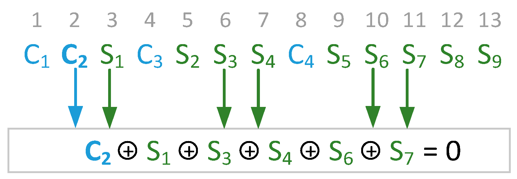
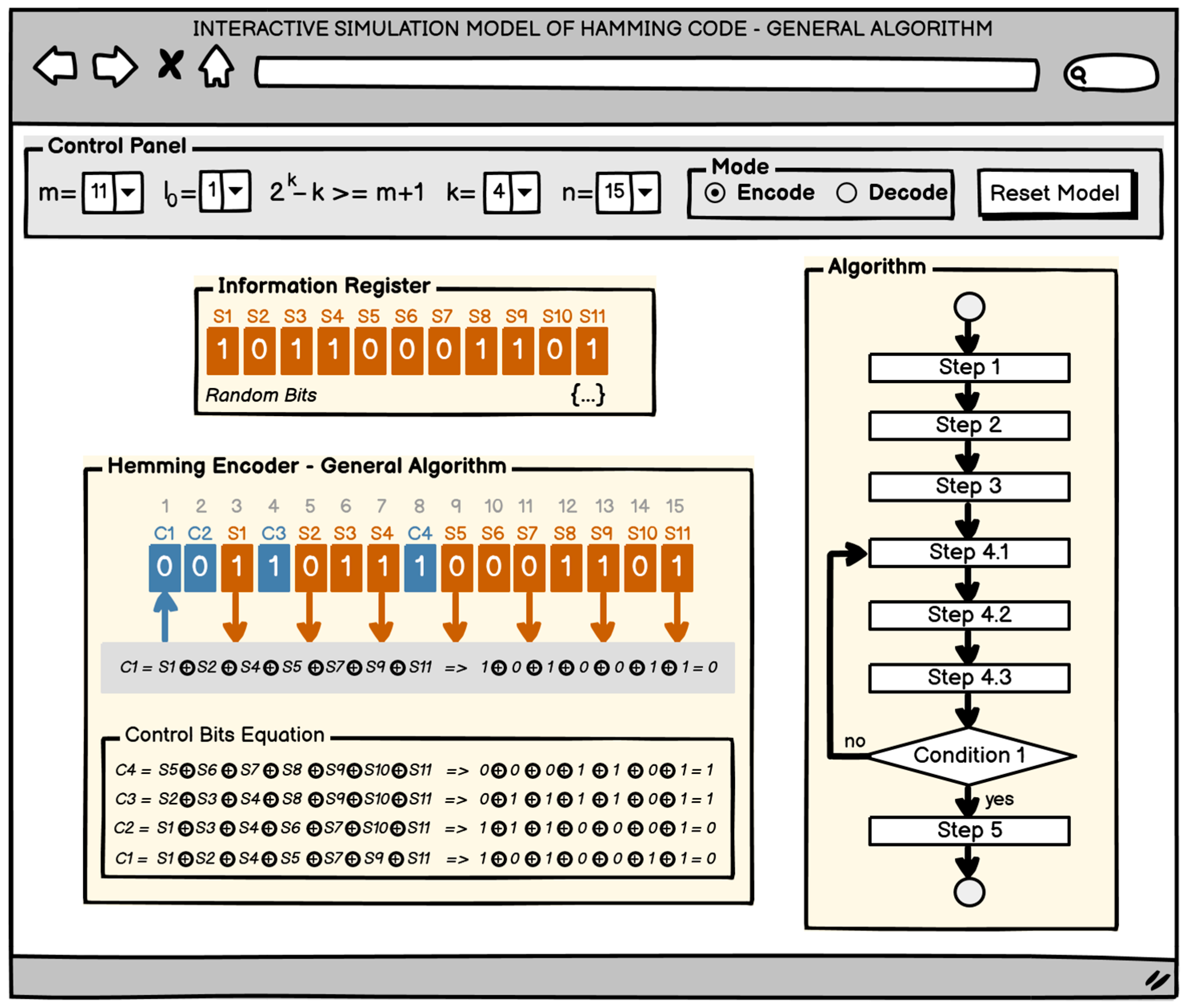
- Formulation of the equation for calculating the control bit (Figure 2). Following the general rule for the equation of the grouping will start from , one bit at a time, through one bit, yielding:Figure 2. Equation of the control bit
![Applsci 15 04231 g002]()


- (2)
- Decoding of code combinations using the Hamming code by the general method
- Error syndrome: => => error indication
- Error position:
- (3)
- Extended Hamming codes by the general method
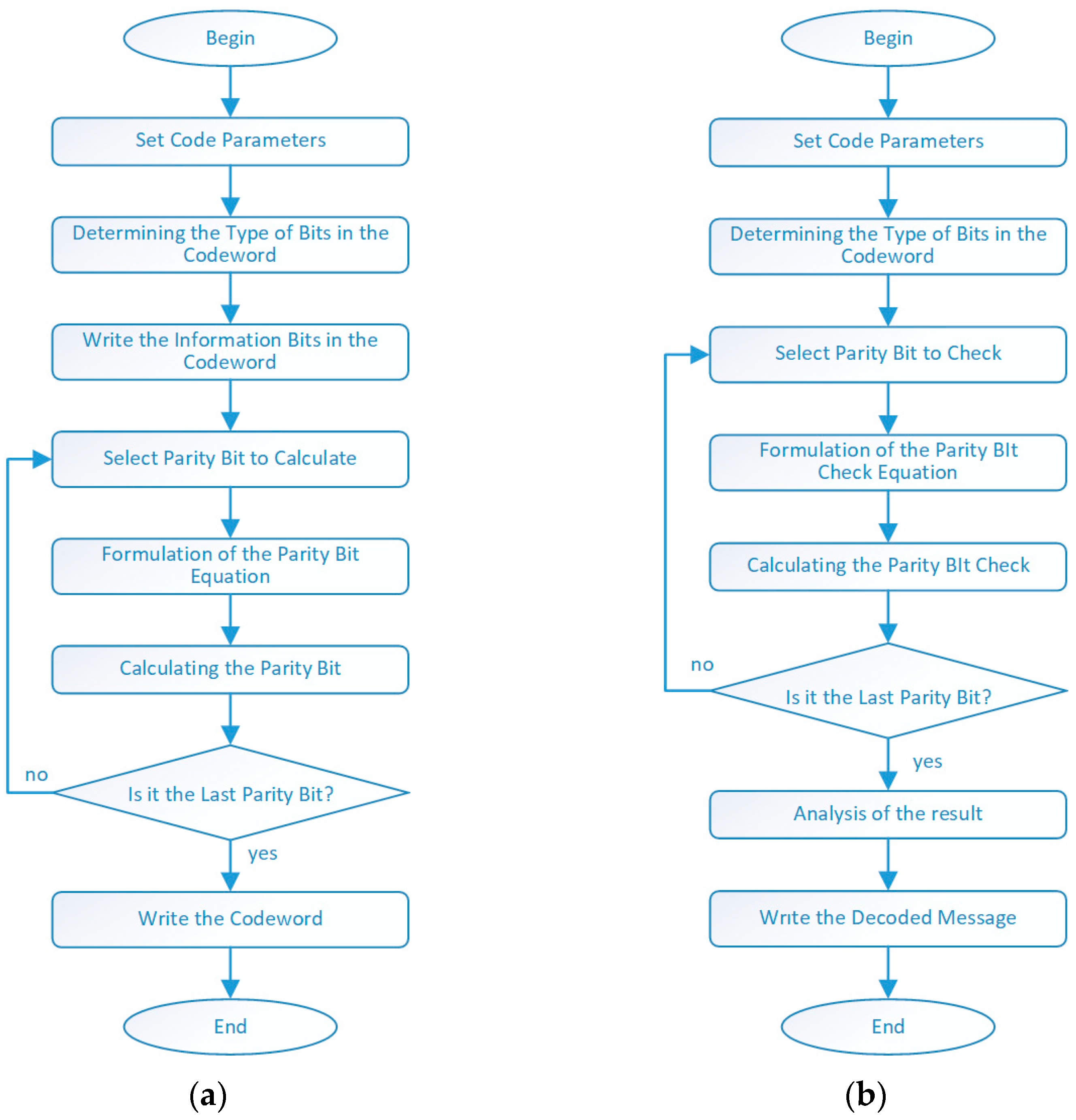
2.2.3. Compiling a Scenario for Solving Hamming Code Problems by the General Method
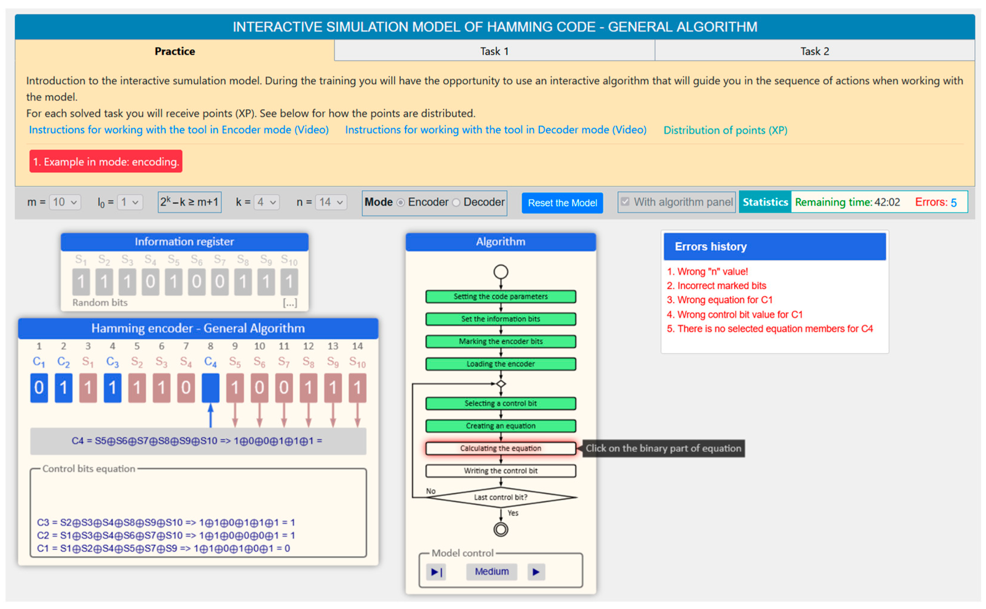
- Encoding mode (Figure 6a)
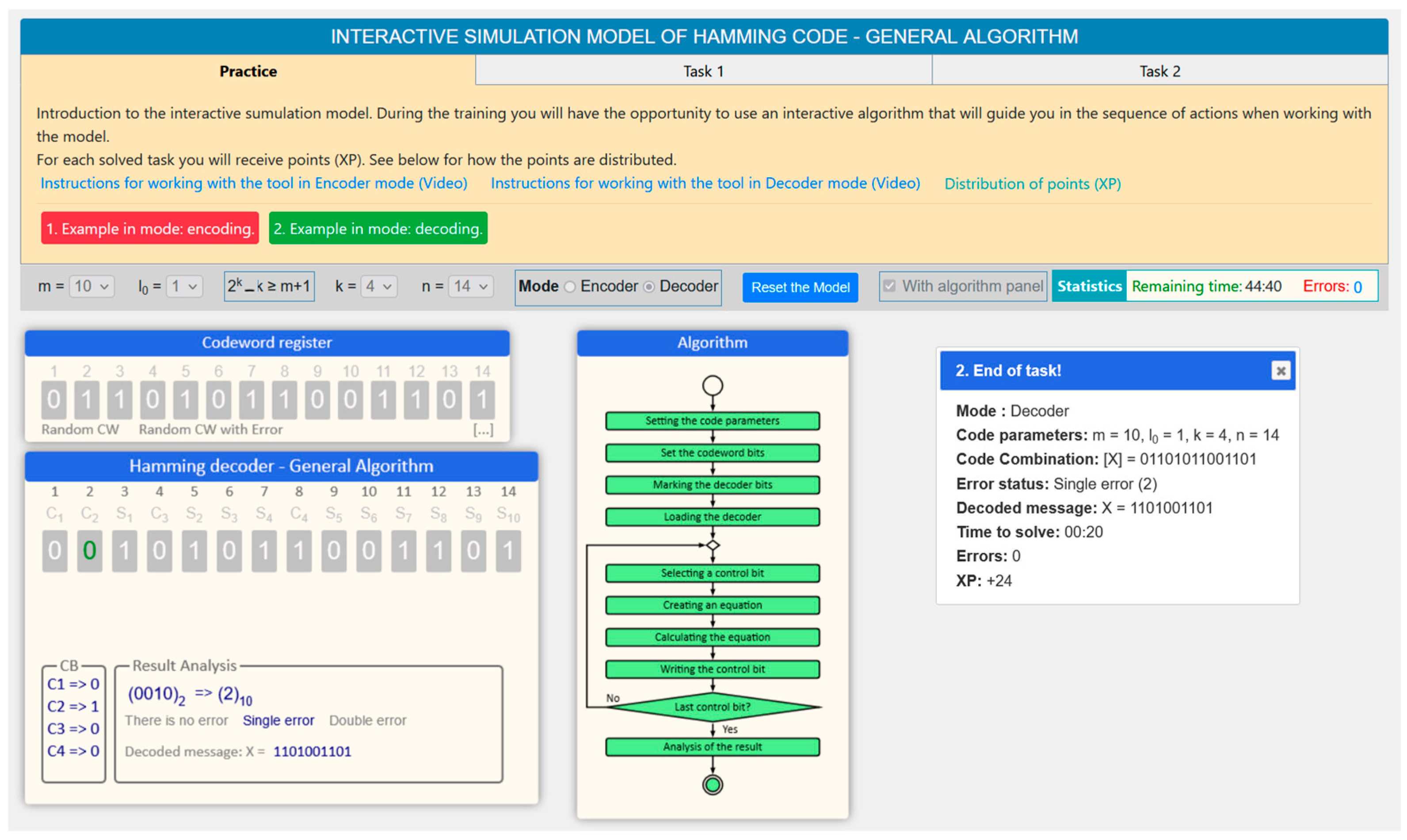
- Decoding Mode—Figure 6b
2.2.4. Formulation of the Requirements for the Interactive Hamming Code Research Model—The General Method
- General requirements for the interactive software models
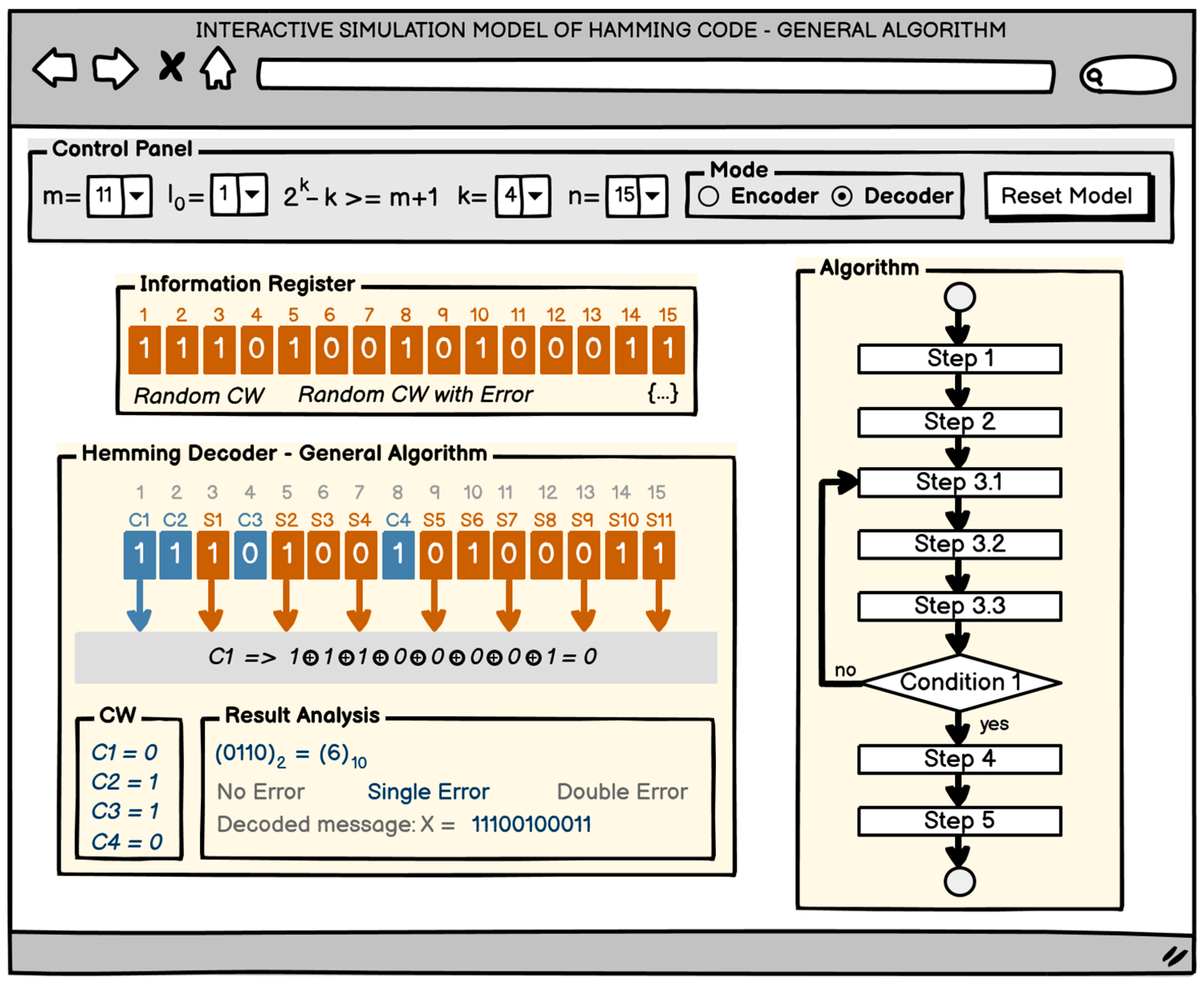
- Control panel. Through this panel, users should be able to set the code parameters ( and ) and operation modes (encoding or decoding), as well as start and stop the model.
- Information register. In the interactive model, a separate panel should be allocated for setting the information bits in the encoding mode (encoder). The information might be entered in the following ways: automatic generation, manual bit-by-bit input, and direct input into a text field.
- Code combination register. This is a panel that should provide the ability to set the code combination in the decoding mode (decoder). The input might be done in the following ways: automatic generation of a correct code combination, automatic generation of a code combination with a random error, manual bit-by-bit input, and direct input into a text field.
- Algorithm. The software model should contain an interactive block diagram in a separate independent panel that shows the working algorithm for solving the researched task. The idea of this block diagram is to show the sequence of steps in solving the task, and when specifying a given block, a short hint for the required action should be displayed. This panel should only be visible in “Training” mode. Individual elements of the flowchart will be visualized in different colors depending on whether the given step has been completed, is currently being completed, or has not yet been completed, i.e.,
- -
- No coloring—the step has not yet been completed;
- -
- Yellow color—the step is currently being executed;
- -
- Green color—step passed successfully.
- Encoder/decoder. A separate panel should be provided where the main actions of the encoding process, resp. decoding process will be carried out, with the corresponding code.
- Statistics. During the operation with the model, statistics must be kept, including the following data:
- -
- Time to solve the task;
- -
- Number of errors made;
- -
- Error history.
- Requirements for the Hamming code research model—the general methodFor the encoding and decoding modes:
- To allow the code combination bits to be marked with appropriate labels (for example, and ).
- To be able to select a control bit, construct an equation with it, and calculate (when encoding) or check (when decoding) its value.For the decoding mode only:
- To be able to set the error syndrome in binary and decimal format.
- To set the error status as one of the following possible situations: “No error”, “Single error”, or “Double error”.
- To be able to determine the decoded binary combination.
2.2.5. User Interface Prototype
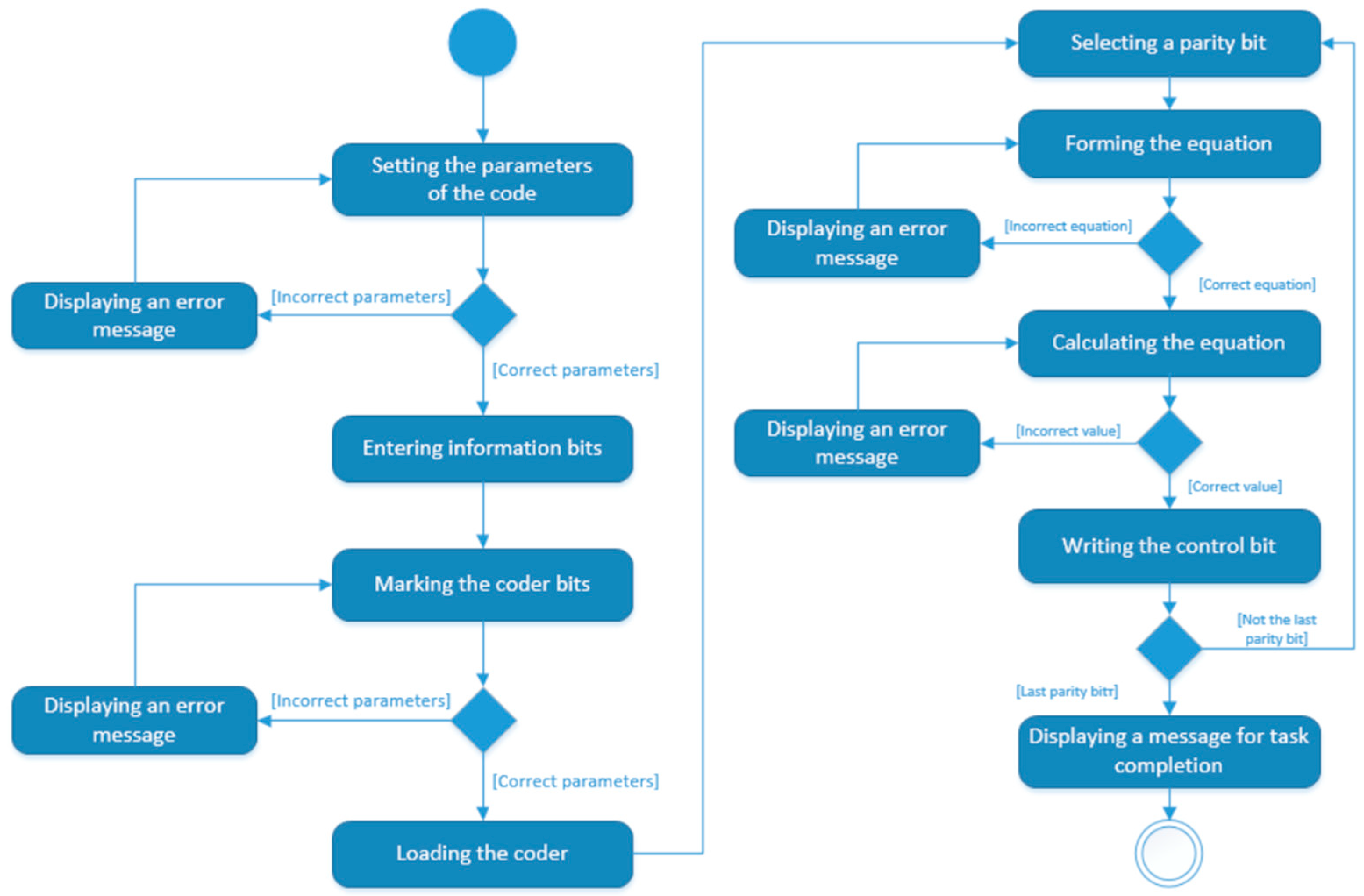
- Graphic layout for the encoding mode
- –
- Marking the bits of the code combination. Initially, the bits of the code combination are undefined and have no values. From a list of pre-generated labels ( and ), the label is selected and placed on the corresponding bit of the code combination by dragging. After correctly marked bits, the bits from the information register are loaded, using a special button, and the control bits have no values at this stage.
- –
- Selecting the control bit. The desired control bit is selected from the code combination by clicking on it.
- –
- Compiling an equation. By clicking on the corresponding bits of the code combination, an equation from the selected labels is automatically filled in a special field, and at the same time after the equation, the bit values are also substituted.
- –
- Calculating the check bit. By clicking on the field with the equation, the value of the expression is written with the substituted values from the equation and the corresponding value is inverted with each click.
- –
- Writing the control bit. Once calculated, writing the value from the equation is done by clicking on the same control bit of the code combination that was selected earlier.
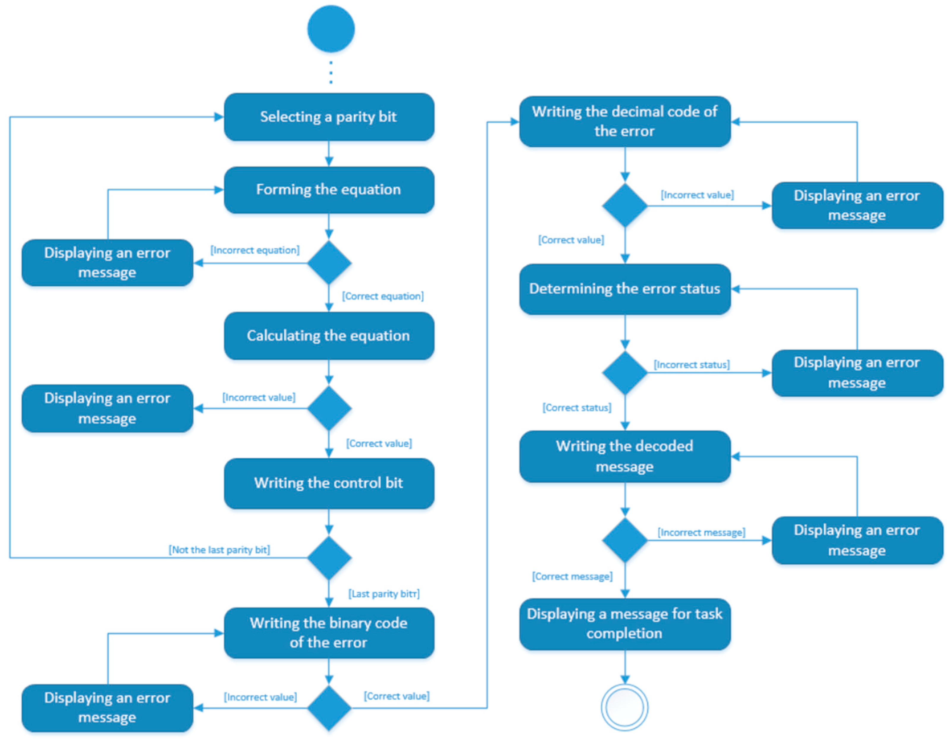
- Graphical layout for the decoding mode
- –
- Select the control bit. The desired control bit is selected from the code combination by clicking.
- –
- Formulating an equation. By clicking on the corresponding bits of the code combination, the equation of the selected bit is automatically filled in a special field, while at the same time, the bit values are replaced after the equation.
- –
- Check bit calculation. After the equation is created, clicking on its field displays the value of the control bit, inverting it with each click.
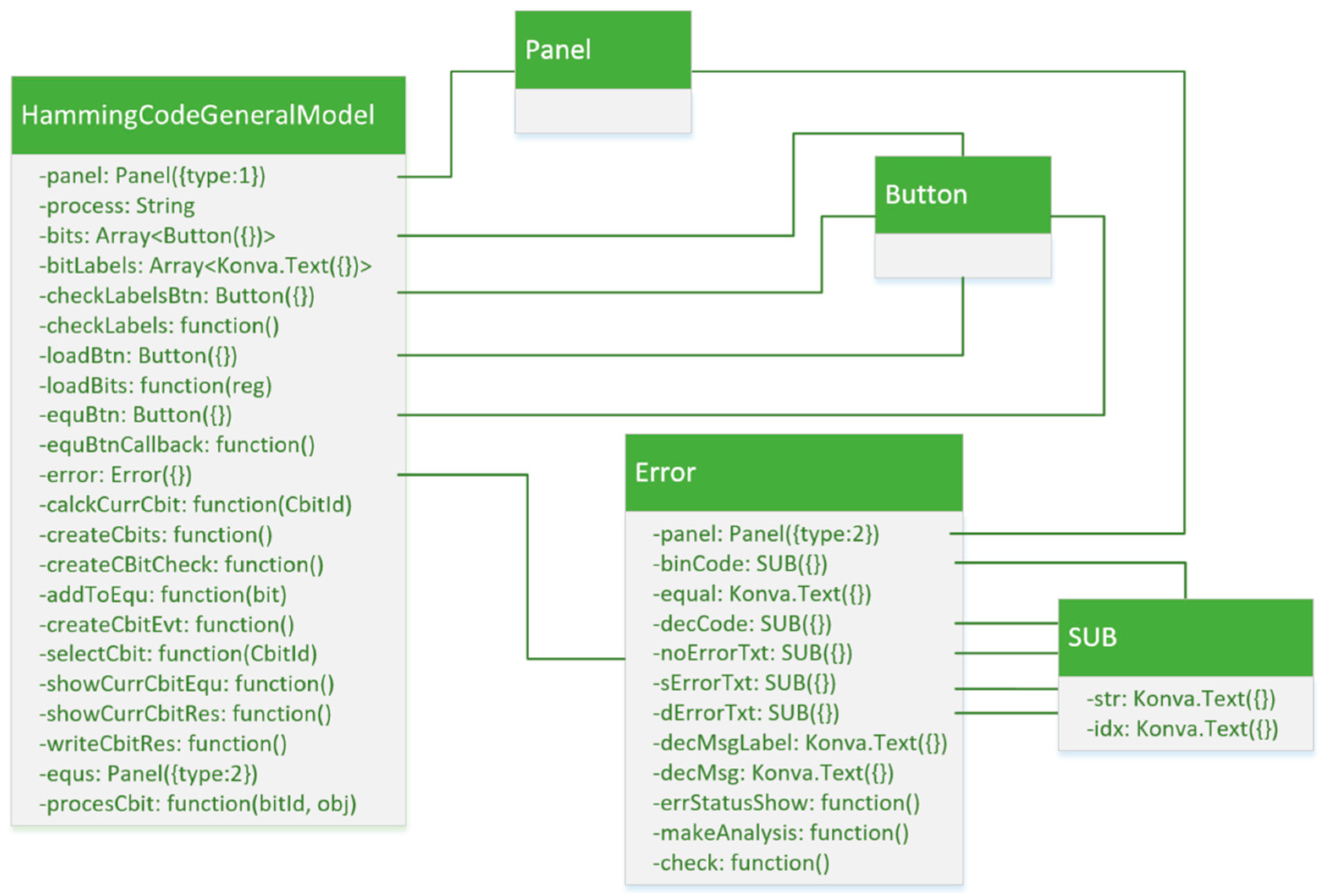
2.3. Creation of the Software Model Code
3. Results
3.1. Implementation of a Software Training Model for Learning Hamming Codes by the General Method
3.2. Software Tool Effectiveness Assessment
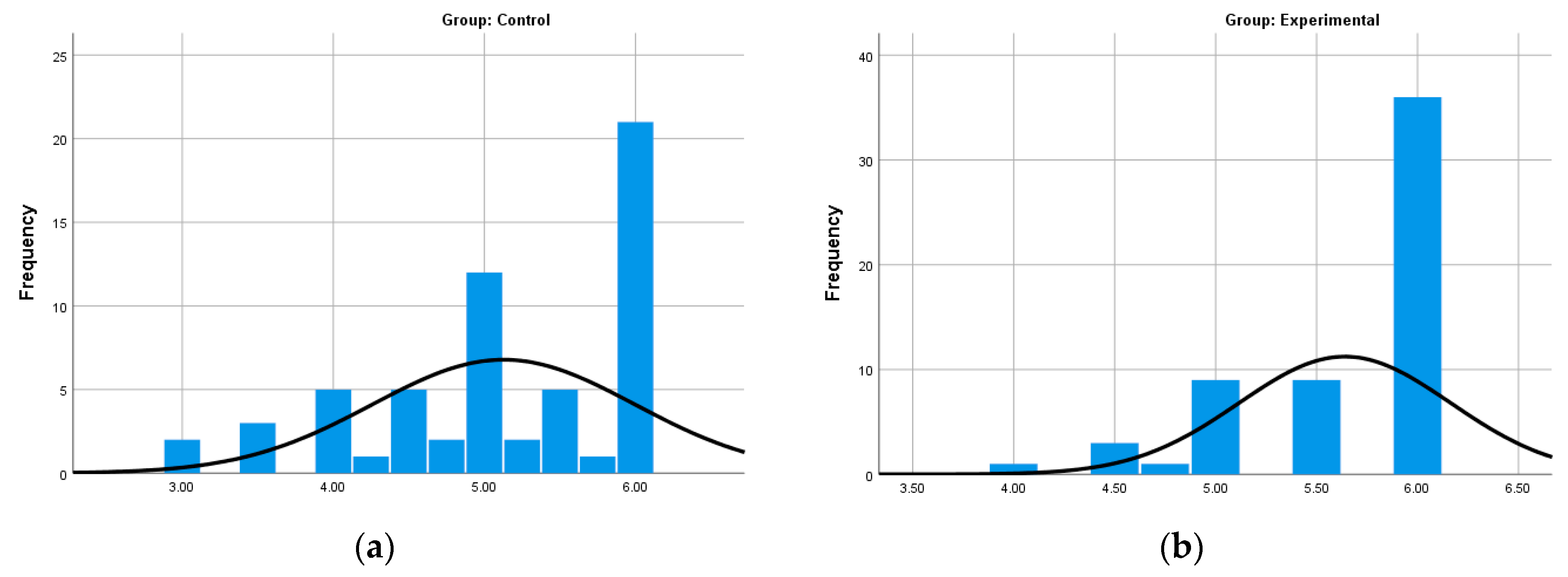
3.2.1. Pedagogical Experiment for Student Success
- Basic statistics
- ANCOVA analysis
- Dependent variable: Assessment (grade) from the control work.
- Independent variable: Group, i.e., learning method (traditional method vs. interactive software).
- Covariates:
- o
- Average grade from the previous two semesters.
- o
- Period (2019–2020 vs. 2021–2022).
- Corrected Model:
- o
- Type III Sum of Squares: 20.328
- o
- df: 4
- o
- Mean Square: 5.082
- o
- F-value: 12.216
- o
- p (Sig.): 0.000
- o
- Partial Eta Squared: 0.302
- Intercept:
- o
- p (Sig.): 0.679.
- AverageGrade:
- o
- Type III Sum of Squares: 7.610
- o
- F-value: 18.294
- o
- p (Sig.): 0.000
- o
- Partial Eta Squared: 0.139
- Year:
- o
- p (Sig.): 0.690, which is above 0.05.
- Gender:
- o
- Type III Sum of Squares: 2.463
- o
- F-value: 5.922
- o
- p (Sig.): 0.017
- o
- Partial Eta Squared: 0.050
- Group:
- o
- Type III Sum of Squares: 2.171
- o
- F-value: 5.218
- o
- p (Sig.): 0.024
- o
- Partial Eta Squared: 0.044
- Error and Total:
- o
- Error: the unexplained variance is 47.008, and the value of the Mean Square Error is 0.416.
- o
- Total: the total sum of squares is 3487.188.
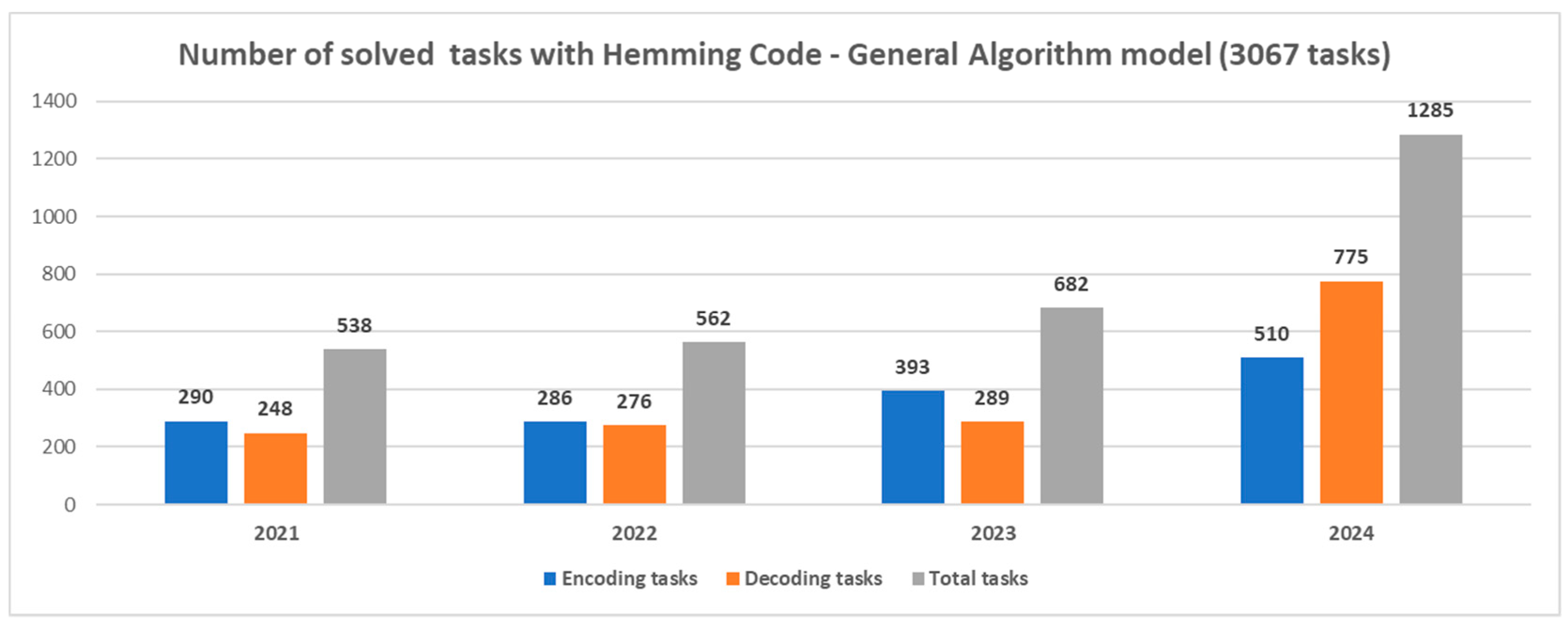
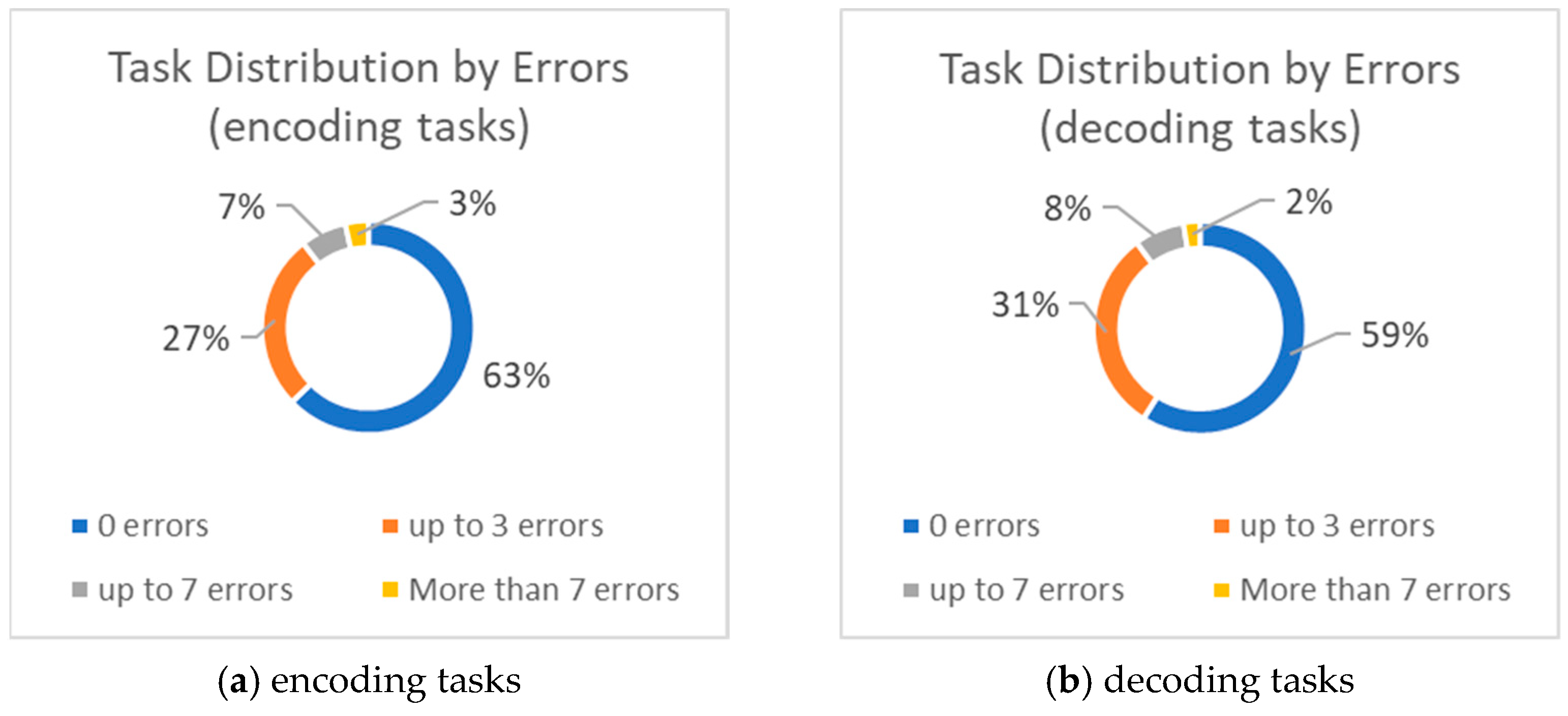
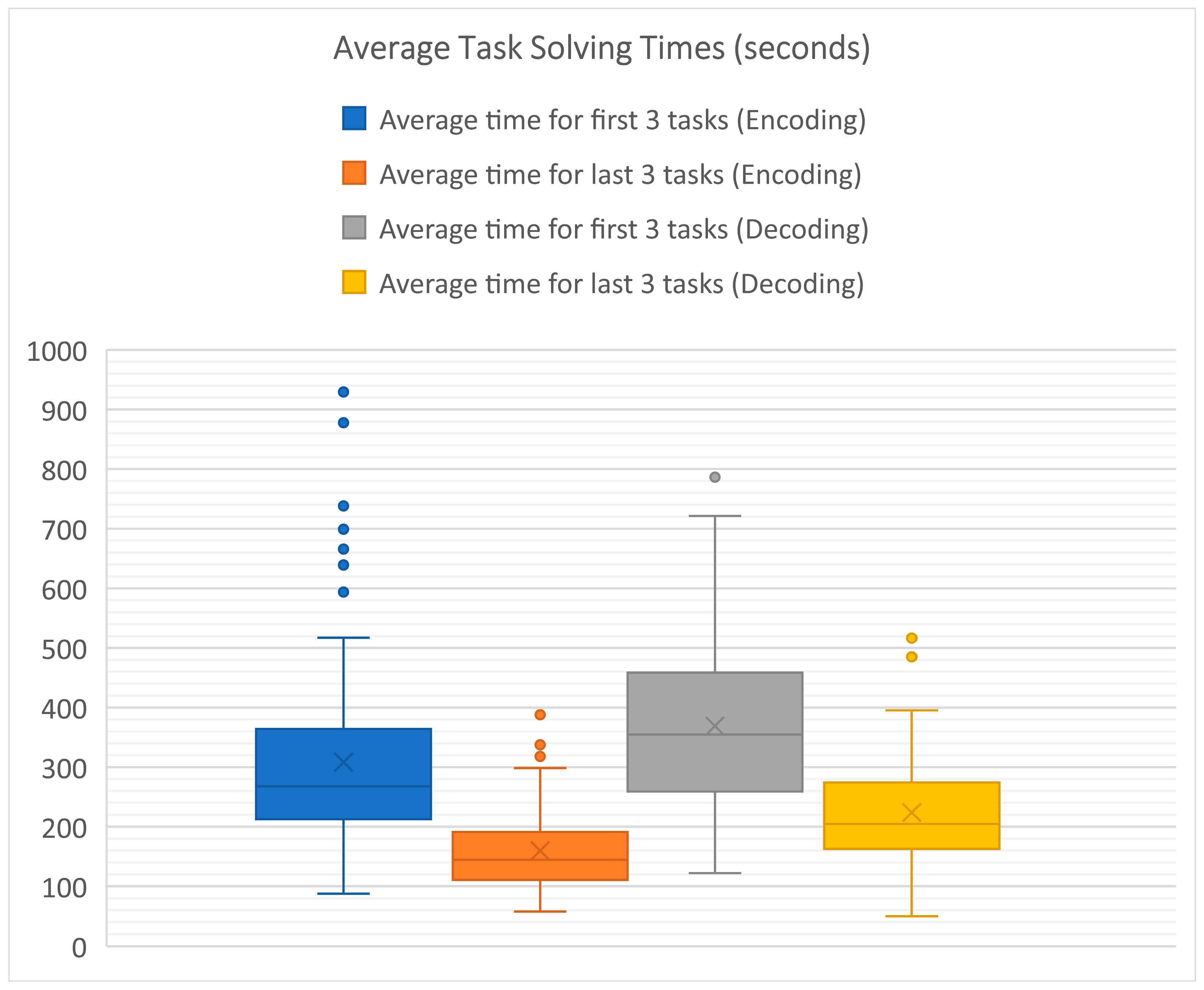
3.2.2. Analysis of Statistical Data on the Usability of the Developed Training Software
3.2.3. Student Satisfaction Assessment Through Survey
4. Discussion
- –
- Expansion of the data set—a collection of more data from different cohorts and educational institutions. This will allow us to assess the effectiveness of interactive software in different educational contexts and to identify the factors that most strongly influence the results.
- –
- Application of advanced statistical methods—using more complex statistical tests for a deeper analysis of the impact of interactive elements on the learning process. More precise measurement of the effect will help to better adapt the methodology to different groups of students.
- –
- Research on additional factors—analysis of the role of cognitive learning styles and the effects of gamification on student motivation and results. A better understanding of these aspects will allow adapting the learning process to the individual needs of students.
- –
- Students will be able to earn badges and medals based on the results achieved.
- –
- Theoretical test questions will be included, which, if answered correctly, will facilitate obtaining higher honors.
- –
- Rankings will be created, reflecting individual achievements and stimulating the competitive element in learning.
5. Conclusions
- –
- Presentation of a universal methodology for designing interactive training tools for coding theory.
- –
- Development and validation of web-based software for working with tasks related to Hamming codes.
- –
- Conducting an experimental study confirming the statistically significant effect of the proposed methodology on learning outcomes.
- –
- Analysis of real data from the use of the software, showing increased engagement and improvement in students’ skills.
- –
- The sample size in the experiment limits the generalizability of the results.
- –
- The uneven distribution of students by gender makes it difficult to analyze this factor.
- –
- The lack of long-term follow-up of student results does not allow conclusions about the long-term impact of the method.
Author Contributions
Funding
Institutional Review Board Statement
Informed Consent Statement
Data Availability Statement
Conflicts of Interest
References
- Adlet, K.; Zhanagul, S.; Tolkin, Y.; Olga, F.; Nazymgul, A.; Kadir, N. Interactive Educational Technologies as a Factor in the Development of the Subjectivity of University Students. World J. Educ. Technol. Curr. Issues 2022, 14, 533–543. [Google Scholar] [CrossRef]
- Rossi, I.V.; de Lima, J.D.; Sabatke, B.; Nunes, M.A.F.; Ramirez, G.E.; Ramirez, M.I. Active learning tools improve the learning outcomes, scientific attitude, and critical thinking in higher education: Experiences in an online course during the COVID-19 pandemic. Biochem. Mol. Biol. Educ. 2021, 49, 888–903. [Google Scholar] [CrossRef] [PubMed]
- Abykanova, B.; Nugumanova, S.; Yelezhanova, S.; Kabylkhamit, Z.; Sabirova, Z. The Use of Interactive Learning Technology in Institutions of Higher Learning. Int. J. Environ. Sci. Educ. 2016, 11, 12528–12539. [Google Scholar]
- Forbes Technology Council. (2024, February 1). Technology-Driven Education: A New Era of Learning. Forbes. Available online: https://www.forbes.com/councils/forbestechcouncil/2024/02/01/technology-driven-education-a-new-era-of-learning/ (accessed on 30 January 2025).
- Mayer, R.E. Multimedia Learning, 2nd ed.; Cambridge University Press: Cambridge, UK, 2009. [Google Scholar]
- Chi, M.T.; Wylie, R. The ICAP Framework: Linking Active Learning to Cognitive Engagement. Educ. Psychol. 2014, 49, 219–243. [Google Scholar] [CrossRef]
- Atanasov, V.; Ivanova, A. A framework for evaluation of web-based learning content. Int. J. Inf. Technol. Secur. 2022, 14, 13–24. [Google Scholar]
- VanLehn, K. The Relative Effectiveness of Human Tutoring, Intelligent Tutoring Systems, and Other Tutoring Systems. Educ. Psychol. 2011, 46, 197–221. [Google Scholar] [CrossRef]
- Deterding, S.; Dixon, D.; Khaled, R.; Nacke, L. From Game Design Elements to Gamefulness: Defining “Gamification”. In Proceedings of the 15th International Academic MindTrek Conference, New York, NY, USA, 28 September 2011; pp. 9–15. [Google Scholar]
- Aliev, Y.; Ivanova, G.; Borodzhieva, A. Design and Research of a Virtual Laboratory for Coding Theory. Appl. Sci. 2024, 14, 1–25. [Google Scholar] [CrossRef]
- Hamming, R.W. Error Detecting and Error Correcting Codes. Bell Syst. Tech. J. 1950, 29, 147–160. [Google Scholar] [CrossRef]
- Morelos-Zaragoza, R.H. The Art of Error Correcting Coding; John Wiley & Sons: Hoboken, NJ, USA, 2006. [Google Scholar]
- Huang, P.-C.; Chang, C.-C.; Li, Y.-H.; Liu, Y. Efficient QR Code Secret Embedding Mechanism Based on Hamming Code. IEEE Access 2020, 8, 86706–86714. [Google Scholar] [CrossRef]
- Martínez-Peñas, U. Hamming and Simplex Codes for the Sum-rank Metric. Des. Codes Cryptogr. 2020, 88, 1521–1539. [Google Scholar] [CrossRef]
- Kim, C.; Shin, D.-K.; Yang, C.-N.; Leng, L. Hybrid Data Hiding Based on AMBTC Using Enhanced Hamming Code. Appl. Sci. 2020, 10, 5336. [Google Scholar] [CrossRef]
- Wang, Y.; Tang, M.; Wang, Z. High-Capacity Adaptive Steganography Based on LSB and Hamming Code. Optik 2020, 213, 164685. [Google Scholar] [CrossRef]
- Shen, L. Exploring the Application and Performance of Extended Hamming Code in IoT Devices. In Proceedings of the 2023 International Conference on Machine Learning and Automation, Adana, Turkey, 18–25 October 2023; EWA Publishing: Oxford, UK, 2023; Volume 32, pp. 71–76. [Google Scholar] [CrossRef]
- Ali, M.M.; Hashim, S.J.; Chaudhary, M.A.; Ferré, G.; Rokhani, F.Z.; Ahmad, Z. A Reviewing Approach to Analyze the Advancements of Error Detection and Correction Codes in Channel Coding with Emphasis on LPWAN and IoT Systems. IEEE Access 2023, 11, 127077–127097. [Google Scholar] [CrossRef]
- MATLAB Communications Toolbox. Available online: https://www.mathworks.com/products/communications.html (accessed on 8 January 2025).
- GNU Octave. Communications Toolbox. Available online: https://octave.org (accessed on 8 January 2025).
- Python Libraries. Available online: https://github.com/veeresht/CommPy (accessed on 8 January 2025).
- Simulink—Simulation and Model-Based Design—MATLAB. Available online: https://www.mathworks.com/products/simulink.html (accessed on 8 January 2025).
- Blahut, R.E. Theory and Practice of Error Control Codes; Addison-Wesley: Reading, MA, USA, 1983; ISBN 978-0-470-84356-7. [Google Scholar]
- Sklar, B. Digital Communications: Fundamentals and Applications; Prentice Hall: Upper Saddle River, NJ, USA, 2001. [Google Scholar]
- Moon, T.K. Error Correction Coding: Mathematical Methods and Algorithms; John Wiley & Sons: Hoboken, NJ, USA, 2005. [Google Scholar]
- Valdez, M.; Ferreira, C.M.; Barbosa, F.P.M. 3D Virtual Laboratory for Teaching Circuit Theory—A Virtual Learning Environment (VLE). In Proceedings of the 51st International Universities’ Power Engineering Conference, Coimbra, Portugal, 6–9 September 2016. [Google Scholar] [CrossRef]
- Esquembre, F. Facilitating the Creation of Virtual and Remote Laboratories for Science and Engineering Education. IFAC-PapersOnLine 2015, 48, 49–58. [Google Scholar] [CrossRef]
- HTML Standards. Available online: https://html.spec.whatwg.org/multipage/ (accessed on 8 January 2025).
- Mackie, S.; Mason, R.; Hibbard, J.; Walker, A. JavaScript: Best Practice; SitePoint Pty. Ltd.: Melbourne, Australia, 2018. [Google Scholar]
- JQuery—JavaScript Library. Available online: https://jquery.com/ (accessed on 8 January 2025).
- Konva.js—HTML5 2d Canvas js Library for Desktop and Mobile Applications. Available online: https://konvajs.org/ (accessed on 8 January 2025).
- Koç, H.; Erdoğan, A.M.; Barjakly, Y.; Peker, S. UML Diagrams in Software Engineering Research: A Systematic Literature Review. Proceedings 2021, 74, 13. [Google Scholar] [CrossRef]
- Field, A. Discovering Statistics Using IBM SPSS Statistics; SAGE Publications Ltd.: Thousand Oaks, CA, USA, 2013. [Google Scholar]
- Rutherford, A. ANOVA and ANCOVA: A GLM Approach; John Wiley & Sons: Hoboken, NJ, USA, 2011. [Google Scholar]
- Newsom, J.T. Analysis of Covariance (ANCOVA). Available online: https://web.pdx.edu/~newsomj/mvclass/ho_ancova.pdf (accessed on 8 January 2025).
- Abdelrasheed, N.S.G.; Sulaiman, M.A.B.A.; Saeed, M.A.; AL-Shahri, H.B. Statistical Analysis Tools: A Review of Implementation and Effectiveness of Teaching English. Int. J. Linguist. Lit. Transl. 2022, 5, 241–246. [Google Scholar] [CrossRef]


| Position number | 1 | 2 | 3 | 4 | 5 | 6 | 7 | 8 | 9 | 10 | 11 | 12 | 13 | 14 | 15 |
| Type of bit |
| 1 | 2 | 3 | 4 | 5 | 6 | 7 | 8 | 9 | 10 | 11 | 12 | 13 | |
|---|---|---|---|---|---|---|---|---|---|---|---|---|---|
| Position number: | 0 | 1 | 2 | 3 | 4 | 5 | 6 | 7 | 8 | 9 | 10 | 11 | 12 | 13 | 14 | 15 |
| Type of bit: |
| (1) | there is no error in the code combination | |
| (2) | there is a single error in the code combination that can be corrected by the syndrome binary code | |
| (3) | in the code combination, there is a single error at the position of , which can be corrected | |
| (4) | there is a double error in the code combination that cannot be corrected |
| Descriptives Average Grade from the Previous Two Semesters | |||||
|---|---|---|---|---|---|
| Group | Control | Experimental | |||
| Statistic | Std. Error | Statistic | Std. Error | ||
| Mean | 4.5829 | 0.10109 | 4.6810 | 0.08408 | |
| 95% Confidence Interval for Mean | Lower Bound | 4.3805 | 4.5127 | ||
| Upper Bound | 4.7852 | 4.8493 | |||
| 5% Trimmed Mean | 4.5778 | 4.6699 | |||
| Median | 4.5000 | 4.6700 | |||
| Variance | 0.603 | 0.417 | |||
| Std. Deviation | 0.77649 | 0.64586 | |||
| Minimum | 3.00 | 3.20 | |||
| Maximum | 6.00 | 6.00 | |||
| Range | 3.00 | 2.80 | |||
| Interquartile Range | 1.34 | 1.00 | |||
| Skewness | 0.209 | 0.311 | 0.131 | 0.311 | |
| Kurtosis | −0.878 | 0.613 | −0.554 | 0.613 | |
| Descriptives Hamming Code GA Average Test Scores | |||||
|---|---|---|---|---|---|
| Group | Control | Experimental | |||
| Statistic | Std. Error | Statistic | Std. Error | ||
| Mean | 5.1271 | 0.11297 | 5.6398 | 0.06818 | |
| 95% Confidence Interval for Mean | Lower Bound | 4.9010 | 5.5033 | ||
| Upper Bound | 5.3533 | 5.7763 | |||
| 5% Trimmed Mean | 5.1879 | 5.6926 | |||
| Median | 5.0000 | 6.0000 | |||
| Variance | 0.753 | 0.274 | |||
| Std. Deviation | 0.86773 | 0.52373 | |||
| Minimum | 3.00 | 4.00 | |||
| Maximum | 6.00 | 6.00 | |||
| Range | 3.00 | 2.00 | |||
| Interquartile Range | 1.50 | 0.50 | |||
| Skewness | −0.735 | 0.311 | −1.274 | 0.311 | |
| Kurtosis | −0.332 | 0.613 | 0.661 | 0.613 | |
| Levene’s Test of Equality of Error Variances a | |||
|---|---|---|---|
| Dependent Variable: Hamming Code GA Average Test Scores | |||
| F | df1 | df2 | Sig. |
| 3.128 | 1 | 116 | 0.080 |
| Tests of Between-Subjects Effects | ||||||
|---|---|---|---|---|---|---|
| Dependent Variable: Hamming Code GA Average Test Scores | ||||||
| Source | Type III Sum of Squares | df | Mean Square | F | Sig. | Partial Eta Squared |
| Corrected Model | 20.328 a | 4 | 5.082 | 12.216 | 0.000 | 0.302 |
| Intercept | 0.072 | 1 | 0.072 | 0.172 | 0.679 | 0.002 |
| AverageGrade | 7.610 | 1 | 7.610 | 18.294 | 0.000 | 0.139 |
| Gender | 2.463 | 1 | 2.463 | 5.922 | 0.017 | 0.050 |
| Year | 0.067 | 1 | 0.067 | 0.160 | 0.690 | 0.001 |
| Group | 2.171 | 1 | 2.171 | 5.218 | 0.024 | 0.044 |
| Error | 47.008 | 113 | 0.416 | |||
| Total | 3487.188 | 118 | ||||
| Corrected Total | 67.335 | 117 | ||||
Disclaimer/Publisher’s Note: The statements, opinions and data contained in all publications are solely those of the individual author(s) and contributor(s) and not of MDPI and/or the editor(s). MDPI and/or the editor(s) disclaim responsibility for any injury to people or property resulting from any ideas, methods, instructions or products referred to in the content. |
© 2025 by the authors. Licensee MDPI, Basel, Switzerland. This article is an open access article distributed under the terms and conditions of the Creative Commons Attribution (CC BY) license (https://creativecommons.org/licenses/by/4.0/).
Share and Cite
Aliev, Y.; Ivanova, G.; Borodzhieva, A. Design and Development of Interactive Software Models for Teaching Coding Theory: A Case Study on Hamming Codes—General Algorithm. Appl. Sci. 2025, 15, 4231. https://doi.org/10.3390/app15084231
Aliev Y, Ivanova G, Borodzhieva A. Design and Development of Interactive Software Models for Teaching Coding Theory: A Case Study on Hamming Codes—General Algorithm. Applied Sciences. 2025; 15(8):4231. https://doi.org/10.3390/app15084231
Chicago/Turabian StyleAliev, Yuksel, Galina Ivanova, and Adriana Borodzhieva. 2025. "Design and Development of Interactive Software Models for Teaching Coding Theory: A Case Study on Hamming Codes—General Algorithm" Applied Sciences 15, no. 8: 4231. https://doi.org/10.3390/app15084231
APA StyleAliev, Y., Ivanova, G., & Borodzhieva, A. (2025). Design and Development of Interactive Software Models for Teaching Coding Theory: A Case Study on Hamming Codes—General Algorithm. Applied Sciences, 15(8), 4231. https://doi.org/10.3390/app15084231