

A Prototype for Computing the Distance of Features of High-Pressure Die-Cast Aluminum Products

 , and
, and
Abstract
1. Introduction
2. Literature Review
2.1. Background
2.2. Related Works
3. Materials and Methods
3.1. Digitizer Environment
3.2. Dataset Preparation
3.3. Training and Testing
3.4. Obtaining Distances
4. Results and Discussion
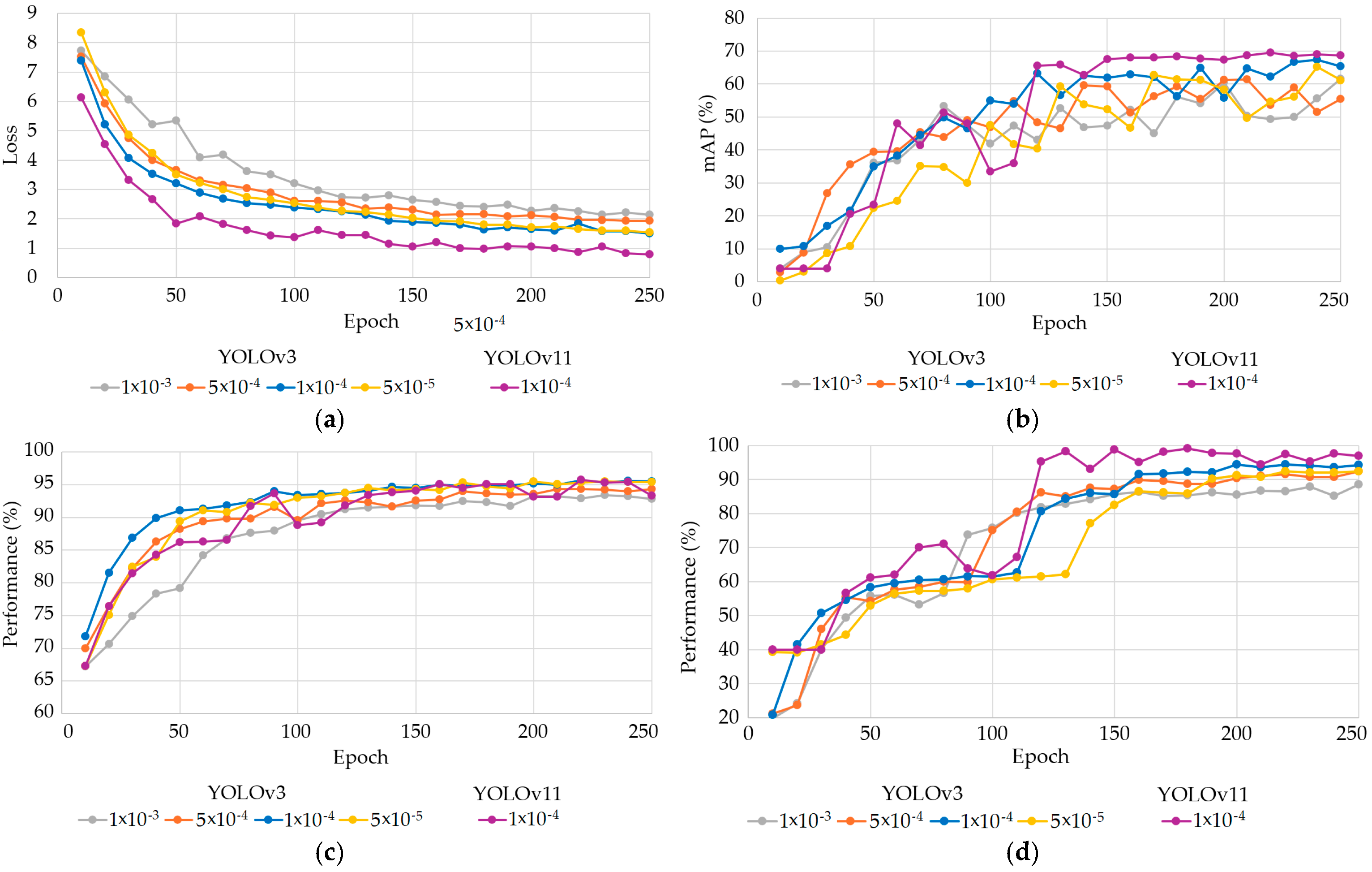
4.1. Training, Validation, and Testing
4.2. Spatial Distances
4.3. On-Site Test with the Prototype
4.4. Discussion
5. Conclusions
Author Contributions
Funding
Data Availability Statement
Acknowledgments
Conflicts of Interest
References
- Börold, A.; Teucke, M.; Rust, J.; Freitag, M. Recognition of car parts in automotive supply chains by combining synthetically generated training data with classical and deep learning based image processing. Procedia CIRP 2020, 93, 377–382. [Google Scholar] [CrossRef]
- Paskert, L. Additive Manufacturing for the Spare Part Management of Classic Cars. Master Thesis, Stellenbosch University, Sudáfrica, South Africa, 2022. [Google Scholar]
- Boissie, K.; Addouche, S.-A.; Baron, C.; Zolghadri, M. Obsolescence management practices overview in automotive industry. IFAC-PapersOnLine 2022, 55, 52–58. [Google Scholar] [CrossRef]
- Zamazal, K.; Denger, A. Product lifecycle management in automotive industry. In Systems Engineering for Automotive Powertrain Development; Hick, H., Küpper, K., Sorger, H., Eds.; Springer: Cham, Switzerland, 2021; pp. 443–469. [Google Scholar] [CrossRef]
- Rosa, E.S.; Godina, R.; Rodrigues, E.M.G.; Matias, J.C.O. An industry 4.0 conceptual model proposal for cable harness testing equipment industry. Procedia Comput. Sci. 2022, 200, 1392–1401. [Google Scholar] [CrossRef]
- AIAG. Potential Failure Mode and Effects Analysis FMEA Reference Manual, 4th ed.; Automotive Industry Action Group: Southfield, MI, USA, 2008. [Google Scholar]
- Kugunavar, S.; Iyer, S.V.; Sangwan, K.S.; Bera, T.C. Data-driven model for CMM probe calibration to enhance efficiency and eustainability. Procedia CIRP 2024, 122, 885–890. [Google Scholar] [CrossRef]
- Luque-Morales, R.A.; Hernandez-Uribe, O.; Mora-Alvarez, Z.A.; Cardenas-Robledo, L.A. Ontology development for knowledge representation of a metrology lab. Eng. Technol. Appl. Sci. Res. 2023, 13, 12348–12353. [Google Scholar] [CrossRef]
- Kiraci, E.; Palit, A.; Attridge, A.; Williams, M.A. The effect of clamping sequence on dimensional variability of a manufactured automotive sheet metal sub-assembly. Int. J. Prod. Res. 2023, 61, 8547–8559. [Google Scholar] [CrossRef]
- Thalmann, R.; Meli, F.; Küng, A. State of the art of tactile micro coordinate metrology. Appl. Sci. 2016, 6, 150. [Google Scholar] [CrossRef]
- Kalajahi, E.G.; Mahboubkhah, M.; Barari, A. On detailed deviation zone evaluation of scanned surfaces for automatic detection of defected regions. Measurement 2023, 221, 113462. [Google Scholar] [CrossRef]
- Dhilleswararao, P.; Boppu, S.; Manikandan, M.S.; Cenkeramaddi, L.R. Efficient hardware architectures for accelerating deep neural networks: Survey. IEEE Access 2022, 10, 131788–131828. [Google Scholar] [CrossRef]
- Adewumi, T.; Liwicki, F.; Liwicki, M. State-of-the-art in open-domain conversational ai: A survey. Information 2022, 13, 298. [Google Scholar] [CrossRef]
- Sharifani, K.; Amini, M. Machine learning and deep learning: A review of methods and applications. World Inf. Technol. Eng. J. 2023, 10, 3897–3904. [Google Scholar]
- Bhatt, D.; Patel, C.; Talsania, H.; Patel, J.; Vaghela, R.; Pandya, S.; Modi, K.; Ghayvat, H. CNN variants for computer vision: History, architecture, application, challenges and future scope. Electronics 2021, 10, 2470. [Google Scholar] [CrossRef]
- Ding, Y.; Luo, X. A virtual construction vehicles and workers dataset with three-dimensional annotations. Eng. Appl. Artif. Intell. 2024, 133, 107964. [Google Scholar] [CrossRef]
- Sui, C.; Jiang, Z.; Higueros, G.; Carlson, D.; Hsu, P.-C. Designing electrodes and electrolytes for batteries by leveraging deep learning. Nano Res. Energy 2024, 3, e9120102. [Google Scholar] [CrossRef]
- He, L.; Li, P.; Zhang, Y.; Jing, H.; Gu, Z. Intelligent control of electric vehicle air conditioning system based on deep reinforcement learning. Appl. Therm. Eng. 2024, 245, 122817. [Google Scholar] [CrossRef]
- Islam, M.R.; Zamil, M.Z.H.; Rayed, M.E.; Kabir, M.M.; Mridha, M.F.; Nishimura, S.; Shin, J. Deep learning and computer vision techniques for enhanced quality control in manufacturing processes. IEEE Access 2024, 12, 121449–121479. [Google Scholar] [CrossRef]
- Junaid, A.; Siddiqi, M.U.R.; Mohammad, R.; Abbasi, M.U. In-process measurement in manufacturing processes. In Functional Reverse Engineering of Machine Tool, 1st ed.; Khan, W.A., Abbas, G., Rahman, K., Hussain, G., Edwin, C.A., Eds.; CRC Press: Boca Raton, FL, USA, 2019; pp. 105–134. [Google Scholar]
- Li, N.; Wang, Z.; Zhao, R.; Yang, K.; Ouyang, R. YOLO-PDC: Algorithm for aluminum surface defect detection based on multiscale enhanced model of YOLOv7. J. Real-Time Image Process. 2025, 22, 86. [Google Scholar] [CrossRef]
- Ercetin, A.; Der, O.; Akkoyun, F.; Gowdru Chandrashekarappa, M.P.; Şener, R.; Çalışan, M.; Olgun, N.; Chate, G.; Bharath, K.N. Review of image processing methods for surface and tool condition assessments in machining. J. Manuf. Mater. Process. 2024, 8, 244. [Google Scholar] [CrossRef]
- Tzampazaki, M.; Zografos, C.; Vrochidou, E.; Papakostas, G.A. Machine vision—Moving from industry 4.0 to industry 5.0. Appl. Sci. 2024, 14, 1471. [Google Scholar] [CrossRef]
- Liu, W.; Li, F.; Jing, C.; Wan, Y.; Su, B.; Helali, M. Recognition and location of typical automotive parts based on the RGB-D camera. Complex Intell. Syst. 2021, 7, 1759–1765. [Google Scholar] [CrossRef]
- Cuesta, E.; Meana, V.; Álvarez, B.J.; Giganto, S.; Martínez-Pellitero, S. Metrology benchmarking of 3D scanning sensors using a ceramic GD&T-based artefact. Sensors 2022, 22, 8596. [Google Scholar] [CrossRef]
- Ren, S.; He, K.; Girshick, R.; Sun, J. Faster R-CNN: Towards real-time object detection with region proposal networks. IEEE Trans. Pattern Anal. Mach. Intell. 2017, 39, 1137–1149. [Google Scholar] [CrossRef]
- Redmon, J.; Divvala, S.; Girshick, R.; Farhadi, A. You Only Look Once: Unified, Real-Time Object Detection. In Proceedings of the Conference on Computer Vision and Pattern Recognition, Las Vegas, NV, USA, 27–30 June 2016. [Google Scholar] [CrossRef]
- Redmon, J.; Farhadi, A. YOLOv3: An incremental improvement. arXiv 2018, arXiv:1804.02767. [Google Scholar] [CrossRef]
- Mery, D. Aluminum casting inspection using deep object detection methods and simulated ellipsoidal defects. Mach. Vis. Appl. 2021, 32, 72. [Google Scholar] [CrossRef]
- Wang, C.-Y.; Bochkovskiy, A.; Liao, H.-Y.M. YOLOv7: Trainable Bag-Of-Freebies Sets new State-Of-The-Art for Real-Time Object Detectors. In Proceedings of the Conference on Computer Vision and Pattern Recognarxition, Vancouver, BC, Canada, 17–24 June 2023. [Google Scholar] [CrossRef]
- Tian, Y.; Ye, Q.; Doermann, D. Yolov12: Attention-centric real-time object detectors. arXiv 2025, arXiv:2502.12524. [Google Scholar] [CrossRef]
- Hussain, M. Yolov1 to v8: Unveiling each variant–a comprehensive review of yolo. IEEE Access 2024, 12, 42816–42833. [Google Scholar] [CrossRef]
- Parlak, İ.E.; Emel, E. Deep learning-based detection of aluminum casting defects and their types. Eng. Appl. Artif. Intell. 2023, 118, 105636. [Google Scholar] [CrossRef]
- Wang, P.; Jing, P. Deep learning-based methods for detecting defects in cast iron parts and surfaces. IET Image Proc. 2024, 18, 47–58. [Google Scholar] [CrossRef]
- Xing, J.; Jia, M. A convolutional neural network-based method for workpiece surface defect detection. Measurement 2021, 176, 109185. [Google Scholar] [CrossRef]
- Duan, L.; Yang, K.; Ruan, L. Research on automatic recognition of casting defects based on deep learning. IEEE Access 2021, 9, 12209–12216. [Google Scholar] [CrossRef]
- Wang, L.; Song, C.; Wan, G.; Cui, S. A surface defect detection method for steel pipe based on improved YOLO. Math. Biosci. Eng. 2024, 21, 3016–3036. [Google Scholar] [CrossRef] [PubMed]
- Terras, N.; Pereira, F.; Ramos Silva, A.; Santos, A.A.; Lopes, A.M.; Silva, A.F.d.; Cartal, L.A.; Apostolescu, T.C.; Badea, F.; Machado, J. Integration of deep learning vision systems in collaborative robotics for real-time applications. Appl. Sci. 2025, 15, 1336. [Google Scholar] [CrossRef]
- Sun, Z.; Caetano, E.; Pereira, S.; Moutinho, C. Employing histogram of oriented gradient to enhance concrete crack detection performance with classification algorithm and Bayesian optimization. Eng. Fail. Anal. 2023, 150, 107351. [Google Scholar] [CrossRef]
- Wang, W.; Chen, Z.; Yuan, X. Simple low-light image enhancement based on Weber–Fechner law in logarithmic space. Signal Process. Image Commun. 2022, 106, 116742. [Google Scholar] [CrossRef]
- Shen, H.; Wei, B.; Ma, Y. Unsupervised anomaly detection for manufacturing product images by significant feature space distance measurement. Mech. Syst. Signal Process. 2024, 212, 111328. [Google Scholar] [CrossRef]
- Mery, D. Aluminum casting inspection using deep learning: A method based on convolutional neural networks. J. Nondestruct. Eval. 2020, 39, 12. [Google Scholar] [CrossRef]
- Nguyen, T.P.; Choi, S.; Park, S.-J.; Park, S.H.; Yoon, J. Inspecting method for defective casting products with convolutional neural network (CNN). Int. J. Precis. Eng. Manuf. Green Technol. 2021, 8, 583–594. [Google Scholar] [CrossRef]
- Brenner, M.; Reyes, N.H.; Susnjak, T.; Barczak, A.L. RGB-D and thermal sensor fusion: A systematic literature review. IEEE Access 2023, 11, 82410–82442. [Google Scholar] [CrossRef]
- Servi, M.; Mussi, E.; Profili, A.; Furferi, R.; Volpe, Y.; Governi, L.; Buonamici, F. Metrological characterization and comparison of D415, D455, L515 RealSense devices in the close range. Sensors 2021, 21, 7770. [Google Scholar] [CrossRef]
- Andriyanov, N.; Khasanshin, I.; Utkin, D.; Gataullin, T.; Ignar, S.; Shumaev, V.; Soloviev, V. Intelligent system for estimation of the spatial position of apples based on YOLOv3 and Real Sense depth camera D415. Symmetry 2022, 14, 148. [Google Scholar] [CrossRef]
- Van Crombrugge, I.; Sels, S.; Ribbens, B.; Steenackers, G.; Penne, R.; Vanlanduit, S. Accuracy assessment of joint angles estimated from 2D and 3D camera measurements. Sensors 2022, 22, 1729. [Google Scholar] [CrossRef] [PubMed]
- Xiang, Y.; Kim, W.; Chen, W.; Ji, J.; Choy, C.; Su, H.; Mottaghi, R.; Guibas, L.; Savarese, S. ObjectNet3D: A Large Scale Database for 3D Object Recognition. In Proceedings of the European Conference on Computer Vision, Amsterdam, The Netherlands, 8–16 October 2016. [Google Scholar] [CrossRef]
- González Izard, S.; Sánchez Torres, R.; Alonso Plaza, Ó.; Juanes Méndez, J.A.; García-Peñalvo, F.J. Nextmed: Automatic imaging segmentation, 3D reconstruction, and 3D model visualization platform using augmented and virtual reality. Sensors 2020, 20, 2962. [Google Scholar] [CrossRef] [PubMed]
- Rajamohan, G.; Sangeeth, P.; Nayak, P.K. On-machine measurement of geometrical deviations on a five-axis CNC machining centre. Adv. Mater. Process. Technol. 2022, 8, 269–281. [Google Scholar] [CrossRef]
- Patel, D.R.; Kiran, M.B. Vision based prediction of surface roughness for end milling. Mater. Today Proc. 2021, 44, 792–796. [Google Scholar] [CrossRef]
- Palani, S.; Natarajan, U. Prediction of surface roughness in CNC end milling by machine vision system using artificial neural network based on 2D Fourier transform. Int. J. Adv. Manuf. Technol. 2011, 54, 1033–1042. [Google Scholar] [CrossRef]
- Jiang, L.; Wang, Y.; Tang, Z.; Miao, Y.; Chen, S. Casting defect detection in X-ray images using convolutional neural networks and attention-guided data augmentation. Measurement 2021, 170, 108736. [Google Scholar] [CrossRef]
- Schlotterbeck, M.; Schulte, L.; Alkhaldi, W.; Krenkel, M.; Toeppe, E.; Tschechne, S.; Wojek, C. Automated defect detection for fast evaluation of real inline CT scans. Nondestruct. Test. Eval. 2020, 35, 266–275. [Google Scholar] [CrossRef]
- Yi-Cheng, L.; Syh-Shiuh, Y. Using Machine Vision to Develop an On-Machine Thread Measurement System for Computer Numerical Control Lathe Machines. In Proceedings of the International Multi-Conference of Engineers and Computer Scientists, Hong Kong, China, 13–15 March 2019. [Google Scholar]
- Pérez, J.; León, J.; Castilla, Y.; Shahrabadi, S.; Anjos, V.; Adão, T.; López, M.Á.G.; Peres, E.; Magalhães, L.; Gonzalez, D.G. A cloud-based 3D real-time inspection platform for industry: A case-study focusing automotive cast iron parts. Procedia Comput. Sci. 2023, 219, 339–344. [Google Scholar] [CrossRef]
- Zou, L.; Fang, H.; Li, Y.; Wu, S. Roughness estimation of high-precision surfaces from line blur functions of reflective images. Measurement 2021, 182, 109677. [Google Scholar] [CrossRef]
- Huang, H.; Peng, X.; Wu, S.; Ou, W.; Hu, X.; Chen, L. An automotive body-in-white welding stud flexible and efficient recognition system. IEEE Access 2025, 13, 51938–51955. [Google Scholar] [CrossRef]
- Khow, Z.J.; Tan, Y.F.; Karim, H.A.; Rashid, H.A.A. Improved YOLOv8 model for a comprehensive approach to object detection and distance estimation. IEEE Access 2024, 12, 63754–63767. [Google Scholar] [CrossRef]
- Gąsienica-Józkowy, J.; Cyganek, B.; Knapik, M.; Głogowski, S.; Przebinda, Ł. Deep learning-based monocular estimation of distance and height for edge devices. Information 2024, 15, 474. [Google Scholar] [CrossRef]
- Huang, H.; Zhou, B.; Cao, S.; Song, T.; Xu, Z.; Jiang, Q. Aluminum reservoir welding surface defect detection method based on three-dimensional vision. Sensors 2025, 25, 664. [Google Scholar] [CrossRef]
- Myśliwiec, P.; Kubit, A.; Szawara, P. Optimization of 2024-T3 aluminum alloy friction stir welding using random forest, XGBoost, and MLP machine learning techniques. Materials 2024, 17, 1452. [Google Scholar] [CrossRef] [PubMed]
- Chen, Y.; Wu, Y. Detection of welding defects tracked by YOLOv4 algorithm. Appl. Sci. 2025, 15, 2026. [Google Scholar] [CrossRef]
- Shao, D.; Liu, Y.; Liu, G.; Wang, N.; Chen, P.; Yu, J.; Liang, G. YOLOv7scb: A small-target object detection method for fire smoke inspection. Fire 2025, 8, 62. [Google Scholar] [CrossRef]


| Feature in Spanish | Feature in English |
|---|---|
| Barreno de fundición | Cast bore |
| Barreno maquinado | Drilled bore |
| Brida maquinada | Machined flange |
| Asiento de tornillo | Screw seat |
| Model | Description | Loss | mAP | Feature Selection | Object Selection |
|---|---|---|---|---|---|
| YOLOv3 | Value (best epoch) | 1.44 (247) | 0.652 (240) | 95.91% (246) | 94.62% (203) |
| Average for last 50 data points | 1.58 | 0.575 | 95.32% | 93.67% | |
| YOLOv11 | Value (best epoch) | 1.02 (243) | 0.613 (203) | 97.54% (220) | 97.69% (240) |
| Average for last 50 data points | 1.16 | 0.628 | 87.62% | 96.22% |
| Feature | Quantity | Detected | Accuracy |
|---|---|---|---|
| Cast Bore | 1 | 1 | 100.0% |
| Drilled Bore | 8 | 6 | 75.0% |
| Screw Seat | 2 | 1 | 50.0% |
| x | y | x | y | z | Calculated D | Specified D | |Error| |
|---|---|---|---|---|---|---|---|
| Pixels | mm | mm | mm | mm | |||
| 188 | 253 | −44 | 31 | 459 | 0.000 | 0.000 | 0.000 |
| 267 | 337 | 50 | 116 | 475 | 127.738 | 128.000 | 0.262 |
| 66 | 286 | −188 | 65 | 466 | 148.125 | 148.000 | 0.125 |
| 66 | 207 | −186 | −18 | 472 | 150.777 | 150.500 | 0.277 |
| 89 | 333 | −159 | 113 | 472 | 141.838 | 142.000 | 0.162 |
| 94 | 193 | −155 | −33 | 465 | 128.269 | 128.00 | 0.269 |
| Feature | Quantity | Detected | Accuracy |
|---|---|---|---|
| Cast Bore | 5 | 2 | 40.0% |
| Drilled Bore | 7 | 7 | 100.0% |
| Screw Seat | 7 | 7 | 100.0% |
| x | y | x | y | z | Calculated D | Specified D | |Error| |
|---|---|---|---|---|---|---|---|
| Pixels | mm | mm | mm | mm | |||
| 225 | 268 | 1 | 42 | 515 | 0.000 | 0.000 | 0.000 |
| 246 | 214 | 23 | −9 | 524 | 56.267 | 56.500 | 0.233 |
| 409 | 325 | 189 | 91 | 541 | 196.021 | 196.000 | 0.021 |
| 419 | 267 | 191 | 37 | 560 | 195.320 | 195.500 | 0.180 |
| 24 | 151 | −232 | −75 | 479 | 263.199 | 263.000 | 0.199 |
| 70 | 332 | −173 | 107 | 494 | 186.928 | 187.000 | 0.072 |
| 173 | 198 | −59 | −27 | 480 | 97.908 | 98.000 | 0.092 |
| Feature | Quantity | Detected | Accuracy |
|---|---|---|---|
| Cast bore | 3 | 3 | 100.0% |
| Drilled bore | 12 | 11 | 91.7% |
| Machined flange | 3 | 1 | 33.3% |
| Screw seat | 6 | 6 | 100.0% |
| x | y | x | y | z | Calculated D | Specified D | |Error| |
|---|---|---|---|---|---|---|---|
| Pixels | mm | mm | mm | mm | |||
| 246 | 357 | 37 | 198 | 303 | 0.000 | 0.000 | 0.000 |
| 272 | 386 | 74 | 221 | 344 | 59.825 | 60.000 | 0.175 |
| 290 | 315 | 113 | 137 | 299 | 97.535 | 97.500 | 0.035 |
| 314 | 355 | 150 | 193 | 309 | 113.270 | 113.000 | 0.270 |
| 424 | 254 | 320 | 42 | 557 | 324.193 | 324.000 | 0.193 |
| 345 | 137 | 201 | −217 | 312 | 364.146 | 364.000 | 0.146 |
| 349 | 21 | 209 | −298 | 309 | 525.010 | 525.000 | 0.010 |
| 352 | 261 | 217 | 55 | 302 | 229.891 | 230.000 | 0.109 |
| 148 | 70 | −127 | −227 | 307 | 455.562 | 455.500 | 0.062 |
| 102 | 348 | −216 | 193 | 282 | 253.919 | 254.000 | 0.081 |
| 120 | 180 | −177 | −66 | 301 | 339.847 | 340.000 | 0.153 |
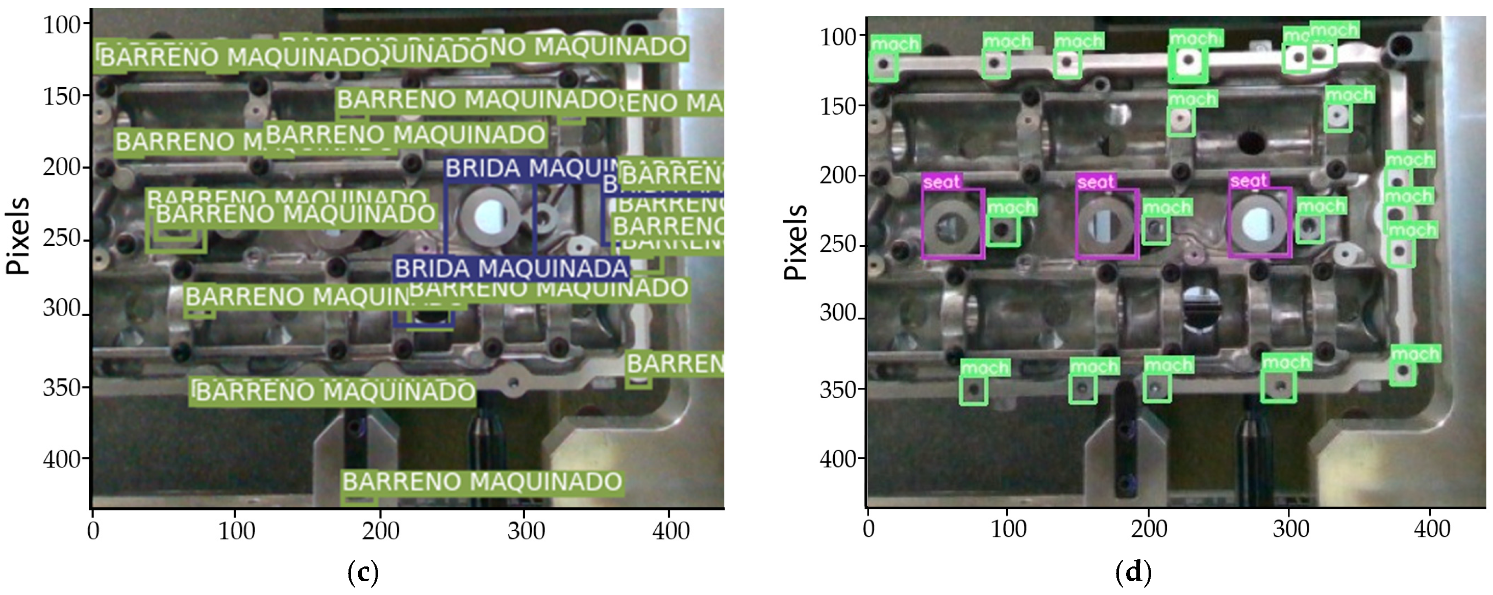
| Feature | Quantity | Detected | Accuracy |
|---|---|---|---|
| Drilled bore: YOLOv3 | 21 | 17 | 80.9% |
| Drilled bore: YOLOv11 | 21 | 19 | 90.5% |
| x | y | x | y | z | Calculated D | Specified D | |Error| | CMM |
|---|---|---|---|---|---|---|---|---|
| Pixels | mm | mm | mm | mm | mm | |||
| 246 | 357 | 37 | 198 | 508 | 0.000 | 0.000 | 0.000 | 0.000 |
| 11 | 122 | −229 | −97 | 515 | 251.970 | 252.000 | 0.030 | 251.866 |
| 25 | 182 | −205 | −38 | 536 | 221.172 | 221.000 | 0.172 | 220.884 |
| 378 | 251 | −168 | 26 | 508 | 164.760 | 165.000 | 0.240 | 164.889 |
| 58 | 235 | −184 | 11 | 501 | 192.172 | 192.000 | 0.172 | 191.787 |
| 76 | 353 | −161 | 123 | 511 | 213.675 | 213.500 | 0.175 | 213.384 |
| 74 | 290 | −157 | 61 | 530 | 179.666 | 179.500 | 0.166 | 179.384 |
| 90 | 123 | −148 | −98 | 504 | 178.779 | 179.000 | 0.221 | 179.014 |
| 129 | 180 | −97 | −40 | 541 | 113.428 | 113.500 | 0.072 | 113.616 |
| 141 | 117 | −92 | −104 | 502 | 137.339 | 137.500 | 0.161 | 137.622 |
| 185 | 419 | −42 | 186 | 512 | 201.102 | 201.000 | 0.102 | 200.893 |
| 180 | 156 | −45 | −61 | 538 | 79.423 | 79.500 | 0.077 | 79.643 |
| 234 | 292 | 11 | 63 | 527 | 74.572 | 74.500 | 0.072 | 74.361 |
| 332 | 157 | 112 | −61 | 534 | 120.021 | 120.000 | 0.021 | 120.111 |
| 374 | 204 | 160 | −19 | 518 | 153.652 | 153.500 | 0.152 | 153.489 |
| 374 | 228 | 161 | 4 | 517 | 154.810 | 155.000 | 0.190 | 155.012 |
| 379 | 337 | 184 | 119 | 471 | 290.026 | 290.000 | 0.026 | 289.879 |
| x | y | x | y | z | Calculated D | Specified D | |Error| | CMM |
|---|---|---|---|---|---|---|---|---|
| Pixels | mm | mm | Mm | mm | mm | |||
| 246 | 357 | 37 | 198 | 508 | 0.000 | 0.000 | 0 | 0.000 |
| 11 | 124 | −230 | −95 | 513 | 252.046 | 252.000 | 0.046 | 251.866 |
| 25 | 183 | −205 | −37 | 536 | 220.924 | 221.000 | 0.076 | 220.884 |
| 378 | 252 | −168 | 27 | 508 | 164.889 | 165.000 | 0.111 | 164.889 |
| 58 | 243 | −184 | 19 | 501 | 192.265 | 192.000 | 0.265 | 191.787 |
| 75 | 351 | −162 | 121 | 511 | 213.738 | 213.500 | 0.238 | 213.384 |
| 74 | 289 | −156 | 60 | 530 | 179.597 | 179.500 | 0.097 | 179.384 |
| 91 | 122 | −146 | −99 | 504 | 178.704 | 179.000 | 0.296 | 179.014 |
| 129 | 180 | −97 | −40 | 541 | 113.265 | 113.500 | 0.235 | 113.616 |
| 141 | 116 | −92 | −105 | 502 | 137.766 | 137.500 | 0.266 | 137.622 |
| 186 | 419 | −41 | 186 | 512 | 200.795 | 201.000 | 0.205 | 200.893 |
| 179 | 157 | −46 | −61 | 538 | 79.753 | 79.500 | 0.253 | 79.643 |
| 235 | 292 | 12 | 63 | 527 | 74.673 | 74.500 | 0.173 | 74.361 |
| 333 | 158 | 113 | −60 | 534 | 120.226 | 120.000 | 0.226 | 120.111 |
| 374 | 204 | 160 | −19 | 518 | 153.723 | 153.500 | 0.223 | 153.489 |
| 374 | 228 | 161 | 4 | 517 | 154.709 | 155.000 | 0.291 | 155.012 |
| 334 | 420 | 118 | 185 | 518 | 210.623 | 210.500 | 0.123 | 210.672 |
| 323 | 405 | 106 | 170 | 519 | 191.044 | 191.000 | 0.044 | 190.994 |
| 379 | 337 | 184 | 119 | 471 | 289.879 | 290.000 | 0.121 | 289.879 |
Disclaimer/Publisher’s Note: The statements, opinions and data contained in all publications are solely those of the individual author(s) and contributor(s) and not of MDPI and/or the editor(s). MDPI and/or the editor(s) disclaim responsibility for any injury to people or property resulting from any ideas, methods, instructions or products referred to in the content. |
© 2025 by the authors. Licensee MDPI, Basel, Switzerland. This article is an open access article distributed under the terms and conditions of the Creative Commons Attribution (CC BY) license (https://creativecommons.org/licenses/by/4.0/).
Share and Cite
Alcántara, L.A.A.; Hernández-Uribe, Ó.; Cárdenas-Robledo, L.A.; Ramírez, J.A.F. A Prototype for Computing the Distance of Features of High-Pressure Die-Cast Aluminum Products. Appl. Sci. 2025, 15, 4230. https://doi.org/10.3390/app15084230
Alcántara LAA, Hernández-Uribe Ó, Cárdenas-Robledo LA, Ramírez JAF. A Prototype for Computing the Distance of Features of High-Pressure Die-Cast Aluminum Products. Applied Sciences. 2025; 15(8):4230. https://doi.org/10.3390/app15084230
Chicago/Turabian StyleAlcántara, Luis Alberto Arroniz, Óscar Hernández-Uribe, Leonor Adriana Cárdenas-Robledo, and José Alejandro Fernández Ramírez. 2025. "A Prototype for Computing the Distance of Features of High-Pressure Die-Cast Aluminum Products" Applied Sciences 15, no. 8: 4230. https://doi.org/10.3390/app15084230
APA StyleAlcántara, L. A. A., Hernández-Uribe, Ó., Cárdenas-Robledo, L. A., & Ramírez, J. A. F. (2025). A Prototype for Computing the Distance of Features of High-Pressure Die-Cast Aluminum Products. Applied Sciences, 15(8), 4230. https://doi.org/10.3390/app15084230