Article

Construction of Simulation System for USV Motion Control and Design of Multi-Mode Controllers Based on VRX and Simulink

1
College of Electrical Engineering, Naval University of Engineering, Wuhan 430033, China
2
Deptartment of Navigation, Naval Petty Officer Academy, Bengbu 233012, China
*
Authors to whom correspondence should be addressed.
Appl. Sci. 2025, 15(8), 4213; https://doi.org/10.3390/app15084213
Submission received: 21 February 2025 / Revised: 31 March 2025 / Accepted: 8 April 2025 / Published: 11 April 2025
(This article belongs to the Section Marine Science and Engineering)

Abstract

:
For the design and verification of a motion control algorithm for unmanned surface vehicles, a simulation system is developed based on VRX and Simulink. Firstly, considering the effect of wind, a dynamic model of the USV with podded propellers is established. Secondly, combined with speed control, three control modes are considered, including yaw rate control, heading control, and path-following control, and speed, heading, yaw rate, and path guidance controllers are designed. Then, a real-time simulation system is developed based on the Virtual RobotX (VRX) environment and the Simulink ROS2 toolbox. Finally, motion control simulation experiments under three control modes and a path-following water tank experiment are carried out. The designed simulation system can simulate the motion of USVs and different environmental elements, such as wind, intuitively and realistically. In simulation experiments, the designed controllers can make the USV follow commands quickly and accurately under three control modes. In the water tank experiment, the USV could stably track the desired path with a relatively small tracking error. Therefore, the effectiveness of the simulation system is strongly confirmed through simulation experiments and the water tank experiment. The simulation system will be expanded in the future for more research on target recognition, path planning, and other aspects of USVs.

1. Introduction

Unmanned surface vehicles (USVs), as unmanned platforms at sea, have been widely used in marine environmental surveys, maritime patrols, reconnaissance, and operations. For example, during the Russia–Ukraine conflict, Ukraine has heavily deployed USVs to carry out various combat missions such as reconnaissance, surveillance, and drone suicide attacks in the Black Sea, which has attracted widespread attention [1]. The design and validation of USV motion control algorithms require navigation tests. However, actual tests have low efficiency and high cost, and in complex sea conditions, the changes in USV model parameters and environmental disturbances pose challenges to the design and verification of motion control algorithms. Therefore, it is important to design simulation systems that are intuitive and realistic to quickly verify the USV motion control algorithms.
At present, USV simulation platforms are mainly divided into digital simulation environments (represented by Simulink) and physical simulation platforms (represented by Gazebo). The former can quickly validate algorithms, but it is difficult to use to intuitively simulate real scenes; physical simulations that support physics engines can conveniently simulate real-world physical phenomena and achieve high-fidelity simulation [2].
Gazebo, as a 3D simulation component of Robot Operating System (ROS), supports various physics engines such as ODE, DART, Bullet, etc., and can simulate various mechanical phenomena, such as the forces acting on USVs in water. Secondly, Gazebo’s modular structure allows for the extension of its core functionality through plugins. By customizing sensor plugins, multiple sensors can be simulated, such as cameras, LiDAR, GNSS, IMU, etc. Xiao et al. [3] designed a virtual simulation platform for USVs based on ROS and Gazebo, considering disturbances such as wind, waves, and currents. Virtual testing experiments were conducted on a certain type of USV to evaluate its perception, trajectory tracking, and autonomous obstacle avoidance performance, verifying the effectiveness of using the platform to test and evaluate USV’s autonomous navigation performance. Paravisi et al. [4] developed the USV simulation platform USVSim based on ROS and Gazebo by improving the hydrodynamic and buoyancy plugins of the underwater robot simulation platform Freefloating, achieving high-fidelity simulation of USV motion under environmental disturbances such as wind, waves, and ocean currents. Fan et al. [2] proposed a comprehensive simulation system for USVs based on USVSim (https://github.com/disaster-robotics-proalertas/usv_sim_lsa accessed on 30 March 2025) and MATLAB (https://www.mathworks.com accessed on 30 March 2025), which meets the requirements for the rapid development and simulation testing of USV navigation control systems.
Virtual RobotX (VRX) is an open-source 3D simulation platform for unmanned surface vessels developed by organizations including the Open Source Robotics Foundation (OSRF). The platform originates from the Maritime RobotX Challenge, which has been held every two years since 2014 and includes tasks such as autonomous path planning, automatic docking, buoy search and detection, and obstacle avoidance [5,6,7]. The current VRX version was developed based on the second-generation robot operating system ROS2 framework. Compared to the TCP/IP-based messaging mechanism of ROS, ROS2 ensures stable data transmission in complex network environments by introducing a DDS (Data Distribution Service) communication mechanism and provides rich QoS (Quality of Service) strategies to meet real-time and security requirements of data transmission in different scenarios [8]. The VRX simulation platform can be used to test algorithms such as detection and recognition, path planning, and motion control for USVs [9,10]. Zhang et al. [11] designed a virtual simulation experimental platform for verifying the motion control program of USVs based on the VRX environment, which exchanged information with external controllers through ROS2. Bayrak et al. [12] designed a simulation platform based on VRX for validating USV path planning algorithms, which can simulate multiple USV scenarios under environmental interference. Meng et al. [13] designed a USV simulation platform based on VRX that integrates path planning and motion control, and verified the effectiveness of their proposed algorithms through the platform.
In recent years, with the widespread application of ROS2, MathWorks has launched a timely ROS toolbox for the graphical programming environment Simulink. Compared to traditional C++ and Python programming, building a control simulation system in Simulink and connecting it to the ROS2 system through the ROS2 module groups in the ROS toolbox is more intuitive and efficient. In addition, Simulink models can be automatically generated into C++ code, compiled into executable programs, and seamlessly deployed in the ROS2 system, thereby achieving full automation from model design to system deployment [14].
Combined with speed control, three control modes are considered in this paper, including yaw rate control, heading control, and path-following control. Using Simulink, speed, heading, yaw rate, and path guidance controllers are designed. The controllers are connected to the ROS2 system using the Simulink ROS Toolbox, and a simulation system for USV motion control combined with the VRX environment is implemented. The main contributions of this paper are as follows:
  • A high-fidelity and plugin-extensible USV motion control simulation system is developed by integrating Simulink with the VRX environment via ROS2, providing a platform for rapid verification of USV motion control algorithms.
  • The feasibility of the proposed simulation system for USV rapid development is validated through path-following water tank experiments, offering an efficient solution to bridge the gap between simulation-based verification and real-world vessel testing of motion control algorithms.

2. USV Dynamic Models

2.1. Reference Frames and Motion Equations
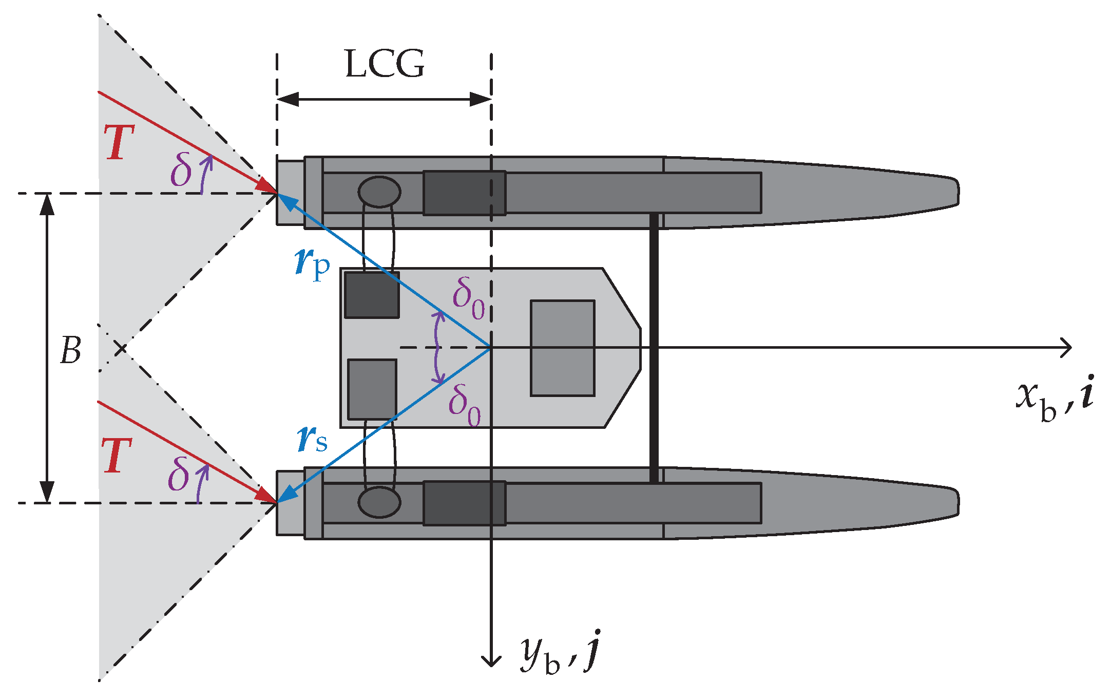
To describe the maneuvering motion of a USV, a geographic reference frame and a body-fixed reference frame are established as shown in Figure 1. The geographic reference frame is fixed to the Earth, pointing North–East–down; the body-fixed reference frame is fixed to the hull, with the origin at the center of gravity of the USV and pointing forward–right–down.
Considering the horizontal motions of a USV, namely, surge, sway, and yaw motions, while neglecting roll, pitch, and heave motions, a simplified three degree of freedom vectorial model for a USV can be expressed as [15]:
η ˙ = J ( η ) ν
M ν ˙ + C ( ν ) ν + D ( ν ) ν = τ + τ wind + τ wave
where η = x y ψ T is the pose vector in the geographic reference frame, containing north position (x), east position (y), and yaw angle (z). ν = u v r T is the velocity vector in the body-fixed reference frame, containing surge velocity (u), sway velocity (v), and yaw rate (r). M is the mass matrix, C ( ν ) is the Coriolis matrix, D ( ν ) is the drag matrix, τ is the vector of forces and moment generated by thrusters, and τ wind and τ wave are the vectors of forces and moment caused by wind and waves, respectively.
Assuming that the hull’s weight is evenly distributed and the hull itself is symmetrical both laterally and longitudinally, J ( η ) , M , C ( ν ) , and D ( ν ) can be expressed, respectively, as follows:
J ( η ) = cos ψ sin ψ 0 sin ψ cos ψ 0 0 0 1
M = m X u ˙ 0 0 0 m Y v ˙ 0 0 0 I z N r ˙
C ( ν ) = 0 0 ( m Y v ˙ ) v 0 0 ( m X u ˙ ) u ( m Y v ˙ ) v ( m X u ˙ ) u 0
D ( ν ) = X u + X u | u | u 0 0 0 Y v + Y v | v | v 0 0 0 N r + N r | r | r
where m is the mass, I z is the moment of inertia about the z b axis, X u ˙ , Y v ˙ , and N r ˙ represent the hydrodynamic added mass, X u , Y v , and N r are the linear damping coefficients, and X u | u | , Y v | v | , and N r | r | are the quadratic damping coefficients.

2.2. Thrust

The thrust vector acting on the USV can be expressed as follows:
τ = T x T y M z T
where T x , T y , and M z are the thrust in the x b and y b directions, and the resulting moment around the z b axis. As shown in Figure 2, the USV designed in this paper provides thrust T p and T s through two podded thrusters at the tail, and the ranges of azimuth angles δ p and δ s are ±45°. We assume that T p = T s = T and δ p = δ s = δ . Therefore, T x , T y , and M z can be, respectively, expressed as follows:
T x = ( T p + T s ) · i = 2 T cos δ
T y = ( T p + T s ) · j = 2 T sin δ
M z = r p × T p + r s × T s = r T sin ( δ 0 δ ) r T sin ( δ 0 + δ ) = LCG · T sin δ
where i and j are the unit vectors in x b and y b directions, respectively. r p = LCG i B / 2 j and r s = LCG i + B / 2 j are the port and starboard moment arms, respectively. LCG is the longitudinal center of gravity, B is the width of the vessel, r is the distance from the center of gravity to the thrusters, δ 0 is the acute angle formed with r p , r s , and x b , and δ 0 = arctan B / 2 LCG .

2.3. Wind Force

The wind force vector acting on the USV can be expressed as follows:
τ wind = q C X ( γ rw ) A Fw C Y ( γ rw ) A Lw C N ( γ rw ) A Lw L
where A Fw and A Lw are the frontal and lateral projected areas of the USV, respectively, L is the length of the vessel, γ rw is the relative attack angle, q is the pressure, and C X , C Y , and C N are the wind coefficients. The formulas are as follows:
q = 1 2 ρ a V rw 2
C X ( γ rw ) = c x cos ( γ rw )
C Y ( γ rw ) = c y sin ( γ rw )
C N ( γ rw ) = c n sin ( 2 γ rw )
where ρ a is the air density, V rw is the relative wind speed, c x , c y , and c n are the coefficients, which are usually taken as 0.5 c x 0.90 , 0.7 c y 0.95 and 0.05 c n 0.20 [16]. If the true wind speed V w , true wind direction β w , surge and sway velocities u and v, and the yaw angle ψ of the USV are known, the components of the relative wind speed V rw along x b and y b can be calculated. The formula is as follows:
u rw = u V w cos ( β w ψ )
v rw = v V w sin ( β w ψ )
Therefore, the formulas for relative wind speed V rw and relative attack angle γ rw are the following:
V rw = u rw 2 + ν rw 2
γ rw = arctan ( ν rw / u rw )

2.4. Wave Model

The wave model adopts the three-dimensional Gerstner model given in [17], and its expression is as follows:
x = x 0 i = 1 N q i A i cos θ i sin k i ( x 0 cos θ i + y 0 sin θ i ) ω t + φ i y = y 0 i = 1 N q i A i sin θ i sin k i ( x 0 cos θ i + y 0 sin θ i ) ω t + φ i z = z 0 i = 1 N A i cos k i ( x 0 cos θ i + y 0 sin θ i ) ω t + φ i
where ( x 0 , y 0 , z 0 ) is the initial position of the particle; q i , A i , θ i , k i , ω i , and φ i , respectively, represent the steepness, amplitude, directional angle, wave number, angular frequency, and initial phase of the ith unit wave. The main energy of waves is concentrated near the peak frequency ω 0 , and the average wave direction angle θ m is considered for the wave direction.
The wave spectrum adopts the Bretschneider spectrum:
S B ( ω ) = 1.25 ω 0 4 H ¯ s 2 4 ω 5 exp 5 4 ω 0 ω 4
where H ¯ s is the significant wave height. Wave gain K H = H ¯ s / H s is introduced, where H s is the significant wave height of a single parameter PM spectrum, described as follows:
S ( ω ) = A / ω 5 · exp ( B / ω 4 )
where A = 8.1 × 10 3 g 2 is a constant, g is the acceleration of gravity, and B = 3.11 / H s 2 . H s and ω 0 satisfy the following expression:
H s = 0.162 g / ω 0 2
Thus, Equation (21) can be expressed as
S B ( ω ) = ( K H ) 2 8.1 × 10 3 g 2 ω 5 exp 5 4 ω 0 ω 4
The relationship between unit wave amplitude A i and S B is as follows:
A i = 2 S B ( ω i ) Δ ω i
where Δ ω i represents the i-th angular frequency interval. At this point, the relationship between wave amplitude A i , wave gain K H , and peak frequency ω 0 has been established. Due to the wave period T 0 = 2 π / ω 0 , the wave model can ultimately be determined using wave gain K H , wave period T 0 , and average wave direction θ m . The wave force vector τ wave is detailed in Algorithm 1 in [17].

3. Controller Design

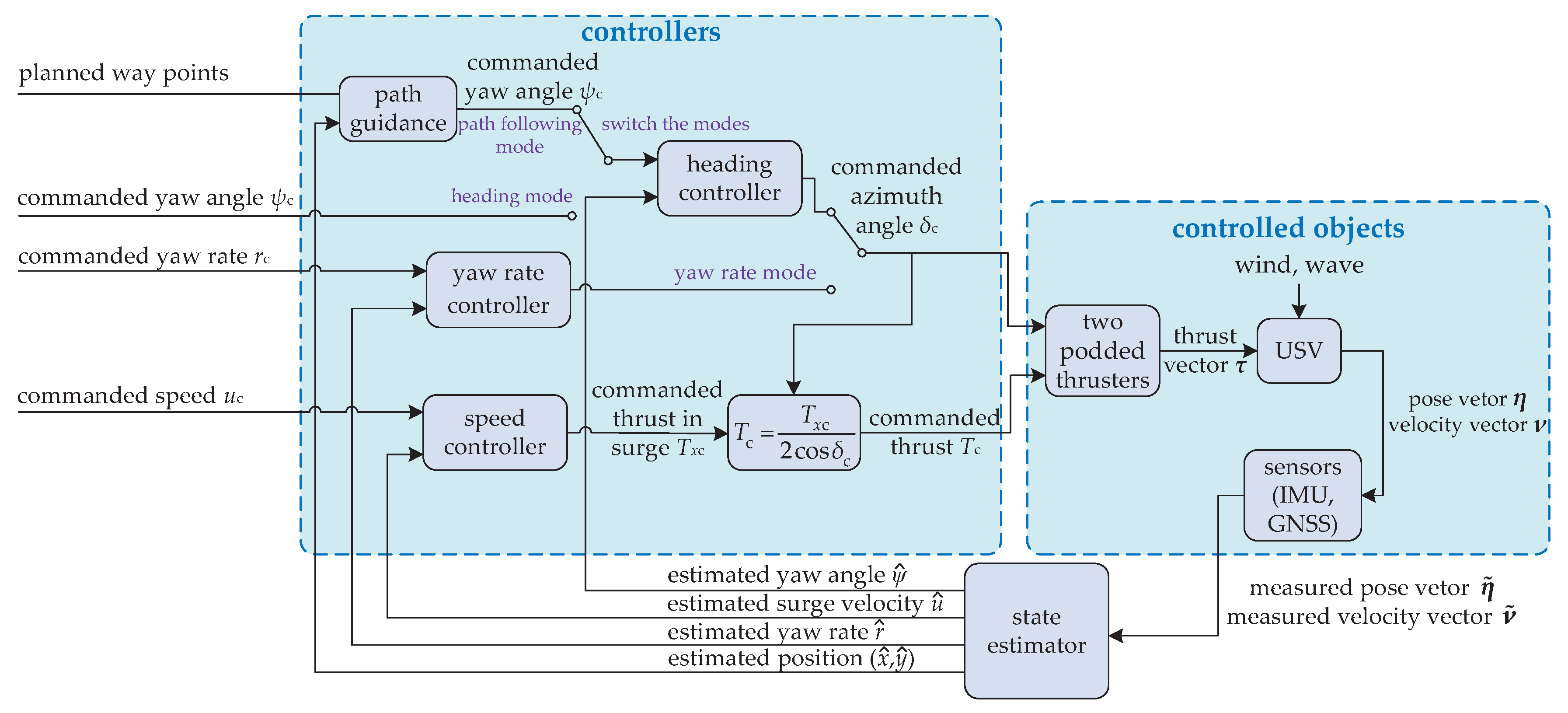
3.1. Control System Architecture

As shown in Figure 3, the USV motion control system consists of three parts: the controllers, the controlled objects, and the state estimator. Among them, the state estimator fuses the measured information from sensors and outputs the estimated values of the USV’s motion status. The controller provides three control modes that combine speed control: yaw rate mode, heading mode, and path-following mode. The speed controller receives the commanded surge velocity u c and estimated surge velocity u ^ , and outputs the commanded thrust in surge T x c . In the yaw rate mode, the yaw rate controller receives the commanded yaw rate r c and estimated yaw rate r ^ , and outputs the commanded azimuth angle δ c . In the heading mode, the heading controller receives a commanded yaw angle ψ c and estimated yaw angle ψ ^ , and outputs δ c . In the path-following mode, the guidance module receives the planned waypoints and estimated vessel position ( x ^ , y ^ ) , calculates the commanded yaw angle ψ c , and outputs it to the heading controller, and then the heading controller outputs δ c . According to T x c and δ c , the commanded thrust T c is calculated from Equation (8). The two podded thrusters receive T c and δ c , and the thrust vector τ containing the thrust and yaw moment is output, thereby achieving motion control of the USV. For the sake of concise writing, in the formulas and simulation curves in the subsequent sections, the symbols η ^ = [ x ^ , y ^ , ψ ^ ] T , and ν ^ = [ u ^ , v ^ , r ^ ] T for the estimated values of the motion parameters will be represented as η = [ x , y , ψ ] T and ν = [ u , v , r ] T , respectively.

3.2. Speed Control

For speed control, including speed control and yaw rate control in the next section, a PI control algorithm based on state feedback is used. Consider the following decoupled model of a marine craft in surge motion:
( m X u ˙ ) u ˙ + X u u + X u | u | u u = T x
The commanded acceleration adopts PI control with acceleration feedforward, and its formula is as follows:
a c u = u ˙ d K p u ( u u d ) K i u 0 t ( u u d ) d τ
Assuming that the commanded thrust is equal to the actual thrust, i.e., T x c = T x , from Equations (26) and (27), and making the state feedback term n ( u ) = X u u + X u | u | u | u | , the following can be obtained:
T x c n ( u ) = ( m X u ˙ ) a c u
Therefore, the commanded thrust in surge motion is
T x c = ( m X u ˙ ) [ u ˙ d K p u ( u u d ) K i u 0 t ( u u d ) d τ ] + n ( u )
According to the pole placement method, the parameters of the PI controller can be obtained as follows:
K p u = 2 λ u
K i u = λ u 2
At this point, the equilibrium point u u d = 0 is globally exponentially stable [15], where λ u = ζ ω n is the designed parameter. The damping ratio ζ (taking ζ = 1 ) and natural frequency ω r of the reference signal should be determined based on expected performance indicators (such as overshoot σ % and adjustment time t s ). Then, ω n should be determined according to the principle that the natural frequency ω n of the closed-loop control system is greater than ω r to complete the design of the control parameters.
The surge velocity reference model adopts a second-order oscillation element, and it can be expressed as
u d u c = ω nu 2 s 2 + 2 ζ u ω nu + ω nu 2
where u d is the reference surge velocity, ζ u is the damping ratio, and ω n u is the natural frequency.

3.3. Yaw Rate Control

The yaw rate controller adopts a PI control algorithm based on state feedback. The first-order Nomoto model can be expressed as
T r ˙ + r = K δ
where K and T are, respectively, the gain and time constant. The commanded angular acceleration adopts PI control with reference feedforward, and its formula is as follows:
a c r = r ˙ d K p r ( r r d ) K i r 0 t ( r r d ) d τ
Therefore, the commanded azimuth angle is
δ c = T / K · [ r ˙ d K p r ( r r d ) K i r 0 t ( r r d ) d τ ] + r / K
The PI controller gain selection is
K p r = 2 λ r
K i r = λ r 2
At this point, the equilibrium point u u d = 0 is globally exponentially stable [15], where λ r > 0 is the designed parameter.
The reference model adopts a second-order oscillation element, and it can be expressed as follows:
r d r c = ω n r 2 s 2 + 2 ζ r ω n r + ω n r 2
where r d is the reference yaw rate, ζ r is the damping ratio, and ω n r is the natural frequency.

3.4. Heading Control
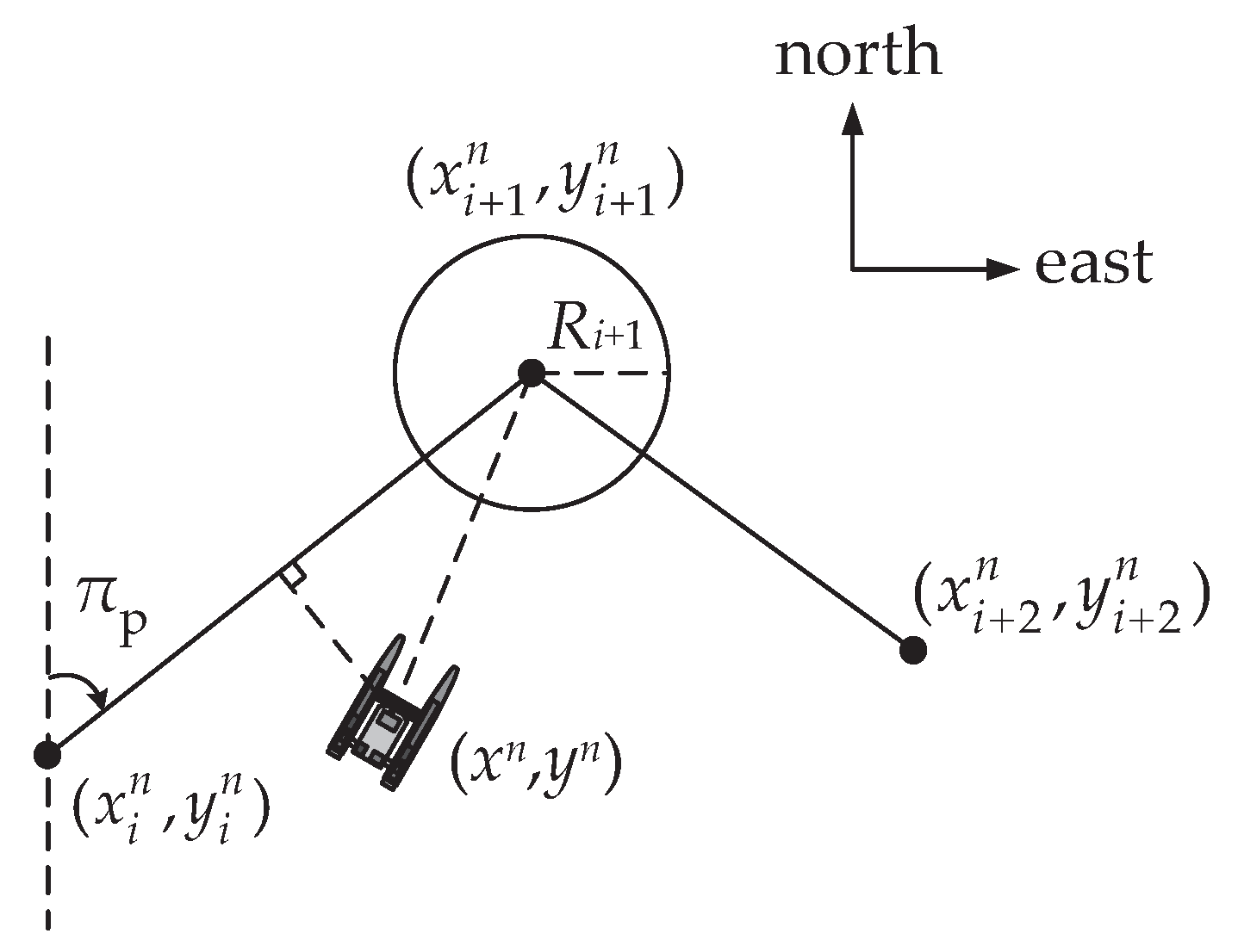
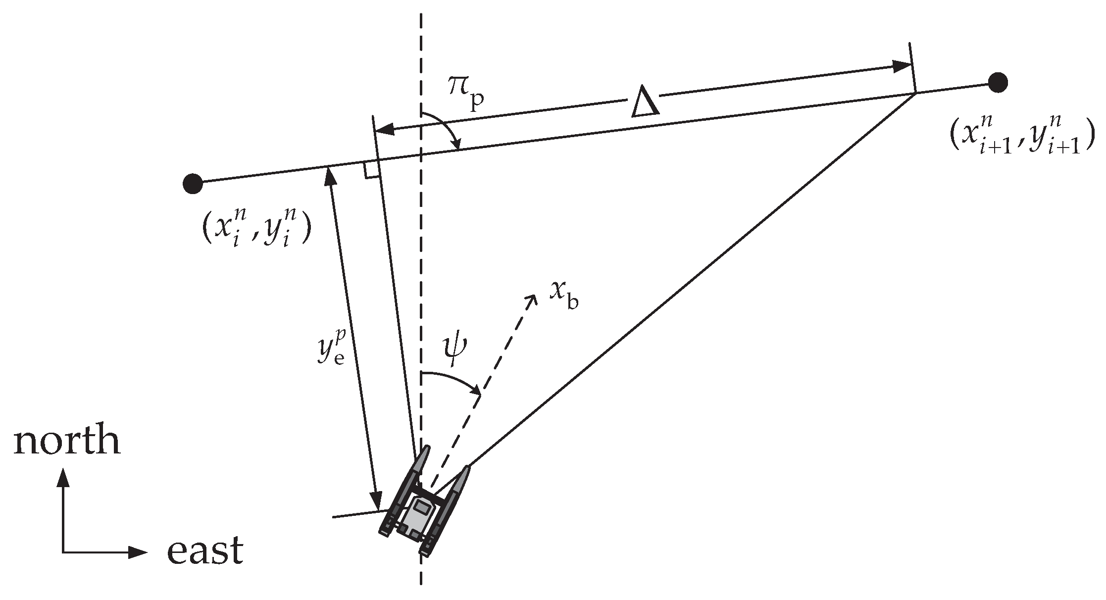
The heading controller adopts the PID control algorithm. Using the first-order Nomoto model, the transfer function from the angle of rotation δ to the yaw angle ψ is as follows:
ψ δ ( s ) = K s ( T s + 1 )
where K and T are both model parameters. The commanded azimuth angle δ c adopts PID control, and its formula is as follows:
δ c = ( K p ψ + K d ψ s + K i ψ 1 s ) ( ψ d ψ )
According to the pole placement method, the parameters of the PID controller can be obtained as follows:
K p ψ = T K ω n ψ 2
K d ψ = T K ( 2 ζ ψ ω n ψ 1 T )
K i ψ = ω n ψ 3 T 10 K
The yaw angle reference model adopts a third-order element, and it can be expressed as follows:
ψ d ψ c = ω nr ψ 3 ( s + ω nr ψ ) ( s 2 + 2 ζ r ψ ω nr ψ s + ω nr ψ 2 )
where ψ d is the reference yaw angle, ζ r ψ is the damping ratio, and ω nr ψ is the natural frequency.

3.5. Path Guidance

As shown in Figure 4, set ( x 1 n , y 1 n ) , , ( x n n , y n n ) as the planned waypoint sequence and adopt a straight segment and acceptance circle switching mechanism—that is, when the vessel enters the acceptance circle, it switches to the next straight segment. The switching condition is the following:
x i + 1 n x n 2 + y i + 1 n y n 2 R i + 1 2
where ( x n , y n ) is the current vessel position, ( x i + 1 n , y i + 1 n ) is the current tracking waypoint, and R i + 1 is the radius of the acceptance circle.
The path guidance module adopts the integral line-of-sight guidance law [15], which can be expressed as
ψ d = π p arctan ( K plos y e p + K ilos y int p )
y ˙ int p = Δ y e p Δ 2 + y e p + κ y int p 2
K plos = 1 / Δ
K ilos = κ K plos
where κ > 0 is the design parameter, π p is the angle between the expected straight path and north direction, y e p is the cross-track error, and Δ is the forward-looking distance, as shown in Figure 5.
Additionally, in the event of guidance signal loss, the heading controller will maintain the current heading, and the path-following mode will degrade to a heading-keeping mode.

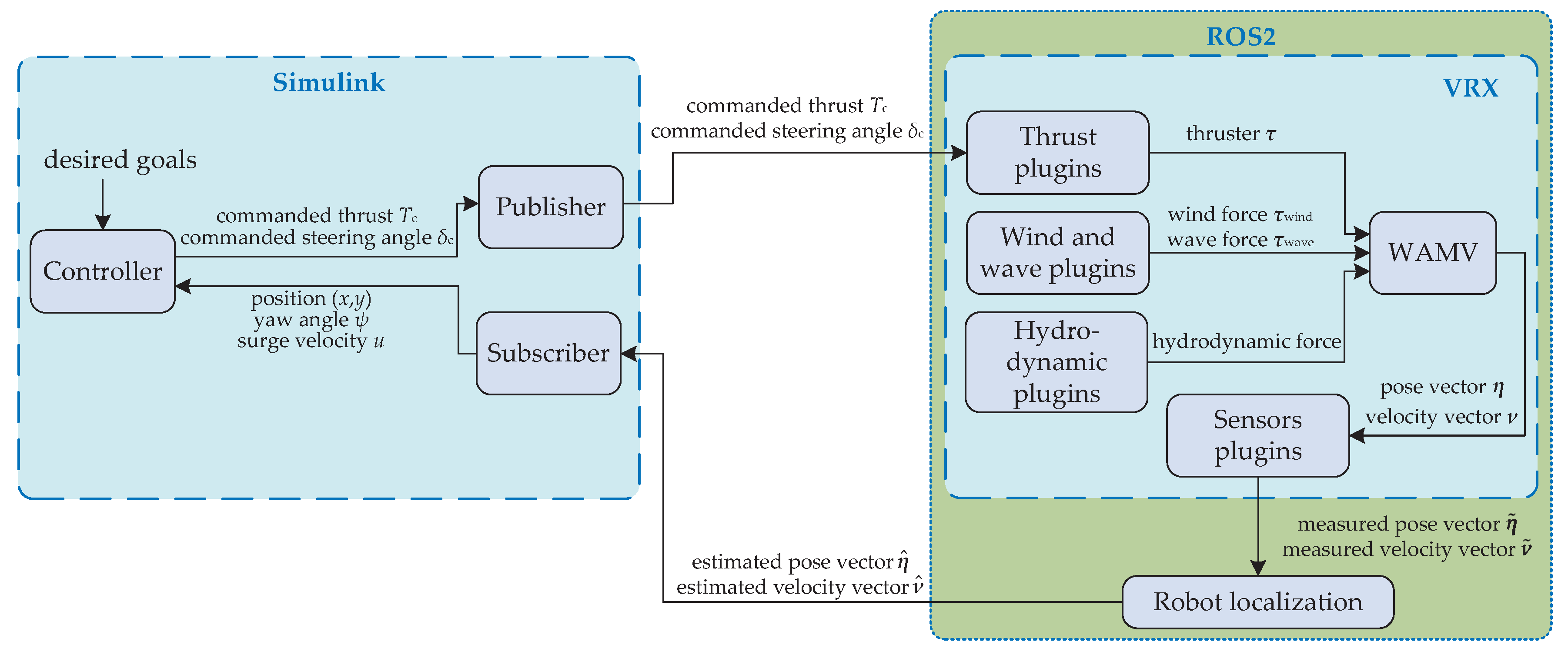
4. Simulation System Design

4.1. Design Scheme

The software configuration of the USV simulation platform designed in this paper is as follows: the Ubuntu 22.04 system; MATLAB R2024a; ROS2 humble. The platform is based on the Virtual RobotX (VRX) environment and uses a wave-adaptive modular vehicle (WAMV) to be simulated in the Gazebo environment.
As shown in Figure 6, the controllers are implemented in Simulink. The controlled object (WAMV) and the motion state feedback are, respectively, implemented by VRX and “robot_localization” [18] in the ROS2 environment. The state estimation package “robot_localization” is used to estimate the motion status of WAMV, providing feedback signals for the controllers. We utilize the Publish and Subscribe modules of the ROS2 module group in the Simulink ROS toolbox to achieve communication between Simulink and VRX.

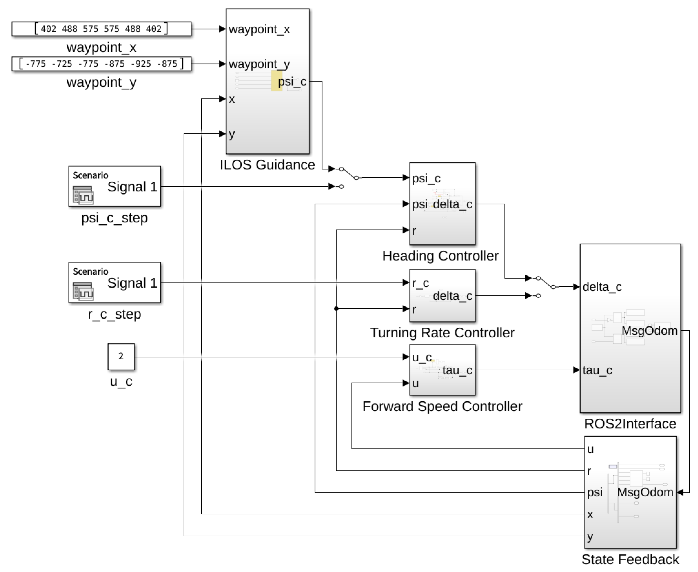
4.2. Controller and ROS2 Interface Modules in Simulink

As shown in Figure 7, the Simulink model includes various commanded signals, guidance modules, various controller modules, and ROS2 interface modules. The ROS2 interface module includes the Publish and Subscribe modules in the Simulink ROS2 toolbox, as shown in Figure 8. The Bus Assignment module receives a blank bus of type std_msg/Float64, as well as commanded thrust T c and azimuth angle δ c , and converts T c and δ c from Simulink signals into ROS2 messages of type std_msgs/Float64.

4.3. VRX Configuration

VRX officially provides a WAMV, which includes two buoys, a power module, a control box, and two thrusters as its basic structure. In addition, a variety of plugins are provided, such as the following: (1) thrust plugins; (2) wind plugins, which can set average wind speed, wind direction, etc. (different parameter settings will generate different wind speeds, simulating the impact of wind on the USV in real scenarios); and (3) wave plugins, which can set wave height and direction, simulating the motion and visual effects of the USV under wave action. The forces calculated by each plugin are synthesized and applied to WAMV through Gazebo’s application programming interface, and the dynamic simulation is implemented through iterative calculation in the physics engine [17].
In addition, users can freely configure sensor modules according to their needs. This design requires obtaining position, attitude, and velocity data; therefore, GNSS and IMU modules need to be configured. The configured WAMV is shown in Figure 9.
The official program provides the dimensions, mass, and various hydrodynamic coefficients of the WAMV. The additional mass is estimated by empirical formulas [19]. A fixed rudder angle δ = 5 is applied to stabilize the rotation of the USV, and the simulation data δ r ( t ) is fitted using the non-linear least-squares method to obtain the parameters K and T in the Nomoto model. The parameters of the WAMV are shown in Table 1. The device errors of the IMU (including the gyroscope and accelerometer) and GNSS are shown in Table 2.

4.4. State Estimator Design

The designed simulation system uses the robot_localization package for motion state estimation. The robot_localization is an open-source package in ROS2 designed for state estimation of moving agents in 3D space. It utilizes two non-linear filtering algorithms—the Extended Kalman Filter (EKF) and the Unscented Kalman Filter (UKF)—to fuse multi-sensor data (e.g., GNSS, IMU, odometry). In this design, the package processes GNSS and IMU measurements of the USV’s motion states using the EKF algorithm to estimate its 3D pose and velocity. Notably, when GNSS signals degrade or are lost, the navigation mode switches to a pure inertial navigation mode based solely on IMU data to ensure continuous output. Upon GNSS signal recovery, the system transitions to a hybrid mode combining GNSS and IMU inputs.

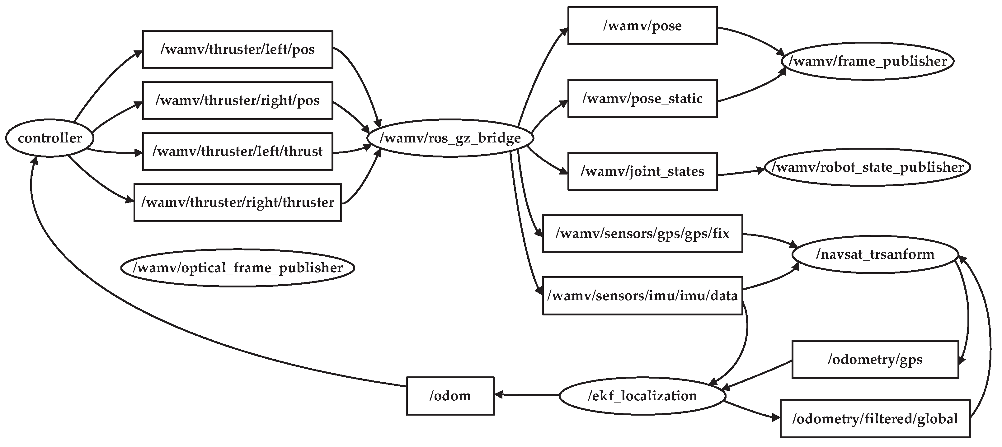
4.5. ROS2 Node and Topic Design

In the ROS2 system, “/controller” is the controller node in Simulink, “/wamv/ros_gz-bridge” is the USV node in VRX, “/navsat_transform” is the transform node of GNSS data, and “/ekf_localization” is the state estimation node. Other nodes such as “/wamv/frame_pubilsher”, “/wamv/robot_state_publisher”, and “/wamv/optical_frame_pubilsher” are nodes related to coordinate transformation. The connection relationship between each node and topic is shown in Figure 10.
The USV node publishes the GNSS and IMU topics “/wamv/sensors/gps/gps/fix” and “/wamv/sensors/imu/imu/data”. The GNSS data conversion node subscribes to these two topics and the “/odometry/filtered/global” topic published by the state estimation node, then publishes the “/odometry/gps” topic (containing GNSS data directly usable by the state estimation node). The state estimation node subscribes to “/odometry/gps” and “/wamv/sensors/imu/imu/data”, performs state estimation, and publishes the odometry topic “/odom” (including position, orientation, linear velocity, angular rate, etc.) for use by the controller node. The controller node subscribes to “/odom” to obtain the corresponding motion status of WAMV, then publishes topics “/wamv/thrusters/left/thrust” and “/wamv/thrusters/right/thrust” (containing commanded thrust T c ) and topics “/wamv/thrusters/left/pos” and “/wamv/thrusters/right/pos” (containing commanded azimuth angle δ c ), which are subscribed to by the USV node.

5. Simulation Results and Water Tank Experiments

5.1. Simulation Results

The simulation verification of the designed controllers is as follows. Start the VRX environment, open Simulink, set the simulation step size and sensor sampling interval to 0.05 s, and run simulations in three modes: yaw rate, heading, and path-following control. Both the yaw rate and heading modes consider two scenarios: no wind, no waves, and wind–wave interference (wind speed 3 m/s, wind direction 90°, wave gain 0.5, wave period 5 s, average wave direction 90°). The parameters of each reference model and controller are shown in Table 3.

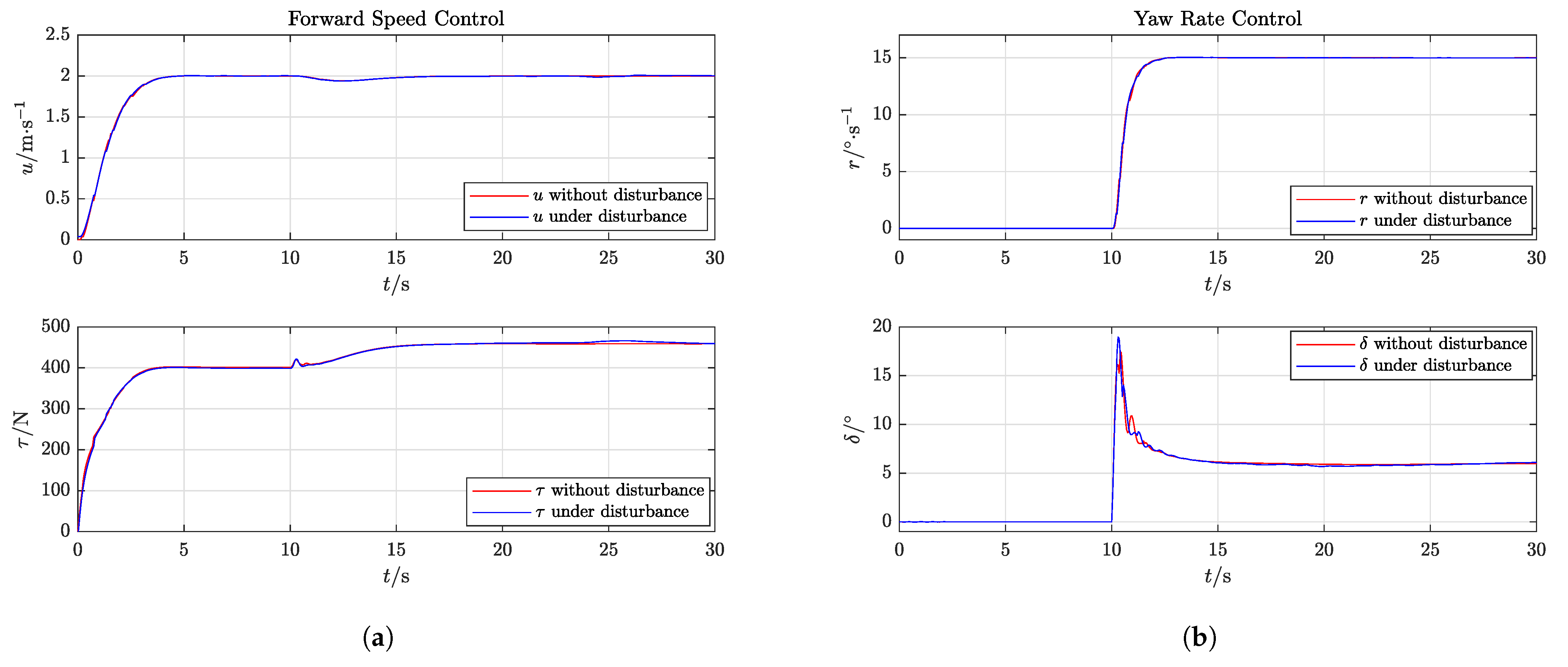
5.1.1. Simulation of Joint Control of Yaw Rate and Surge Velocity

In the yaw rate control mode, the initial surge velocity and yaw rate are both 0. The surge velocity is set to 2 m/s and the yaw rate is set to 15°/s at 10 s. Figure 11a shows the variation curves of surge velocity and thrust, while Figure 11b shows the variation curves of yaw rate and azimuth angle. The red and blue lines correspond to the absence of wind and wave interference and the presence of wind and wave interference, respectively.
As shown in the figure, regardless of the presence or absence of wind and waves, the surge velocity and yaw rate can track the given values without steady-state errors or overshoot. The surge velocity adjustment time is 3.8 s, and the yaw rate adjustment time is 1.9 s. During the acceleration process, the thrust steadily increases, and remains constant during direct navigation at a surge velocity of 2 m/s; when turning, the thrust increases to maintain a constant surge velocity of 2 m/s. The azimuth angle can quickly increase when the yaw rate increases, and maintain a fixed angle required to maintain stable rotation.

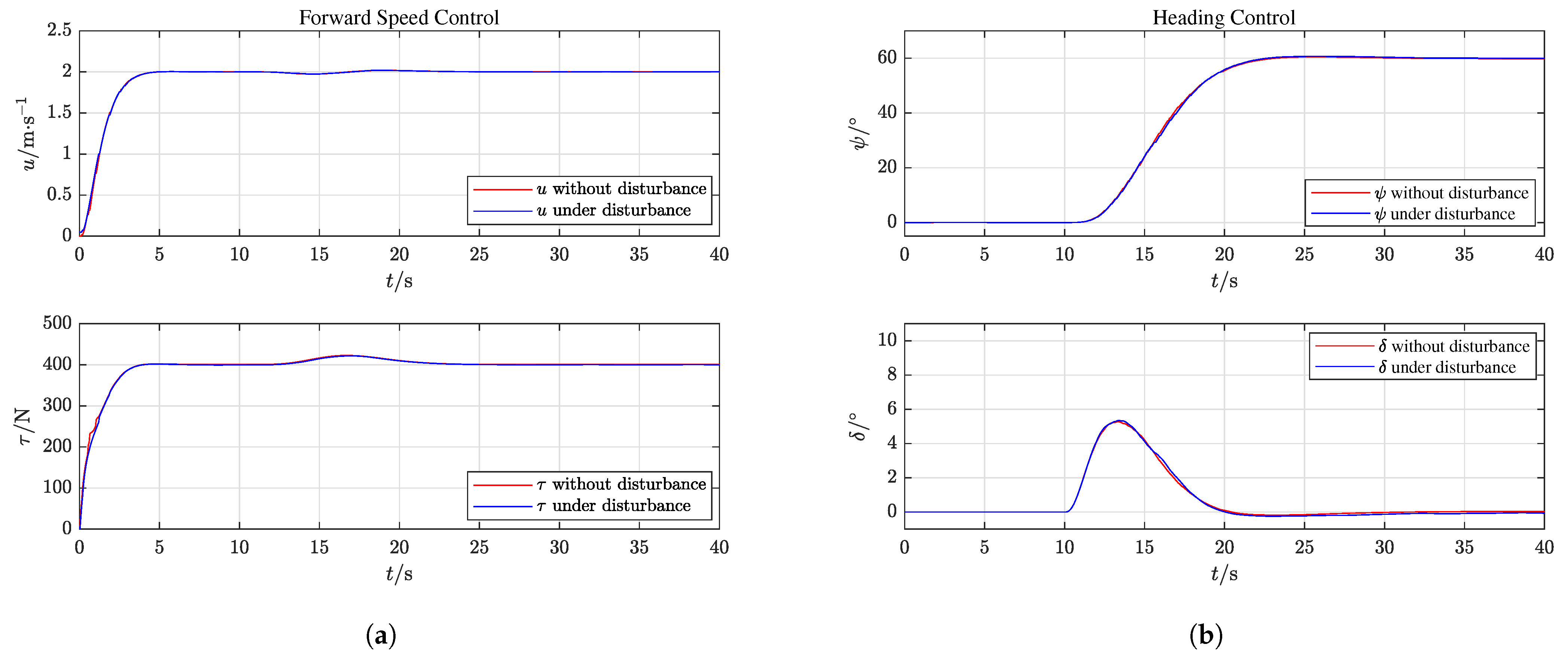
5.1.2. Simulation of Joint Control of Heading and Surge Velocity

In the heading control mode, the initial surge velocity and yaw angle are both 0. The surge velocity is set to 2 m/s, and the yaw angle is set to 60° at 10 s. Figure 12a shows the variation curves of surge velocity and thrust, while Figure 12b shows the variation curves of yaw angle and azimuth angle. The red and blue lines correspond to the absence of wind and wave interference and the presence of wind and wave interference, respectively.
As shown in the figure, regardless of the presence or absence of wind and waves, the surge velocity and yaw angle can track the given values without steady-state errors or oscillations. The surge velocity performance indicators are the same as those described in Section 4.1. When there is no wind or wave interference, the yaw angle overshoot values are 0.8% and 1.1%, respectively, and the adjustment times are 11.8 s and 11.5 s. When starting to turn, the thrust steadily increases; when the turn is completed and direct navigation is resumed, the thrust returns to its original value. When turning, the azimuth angle quickly increases to 5° to change the yaw angle, with a smooth and small amplitude change.

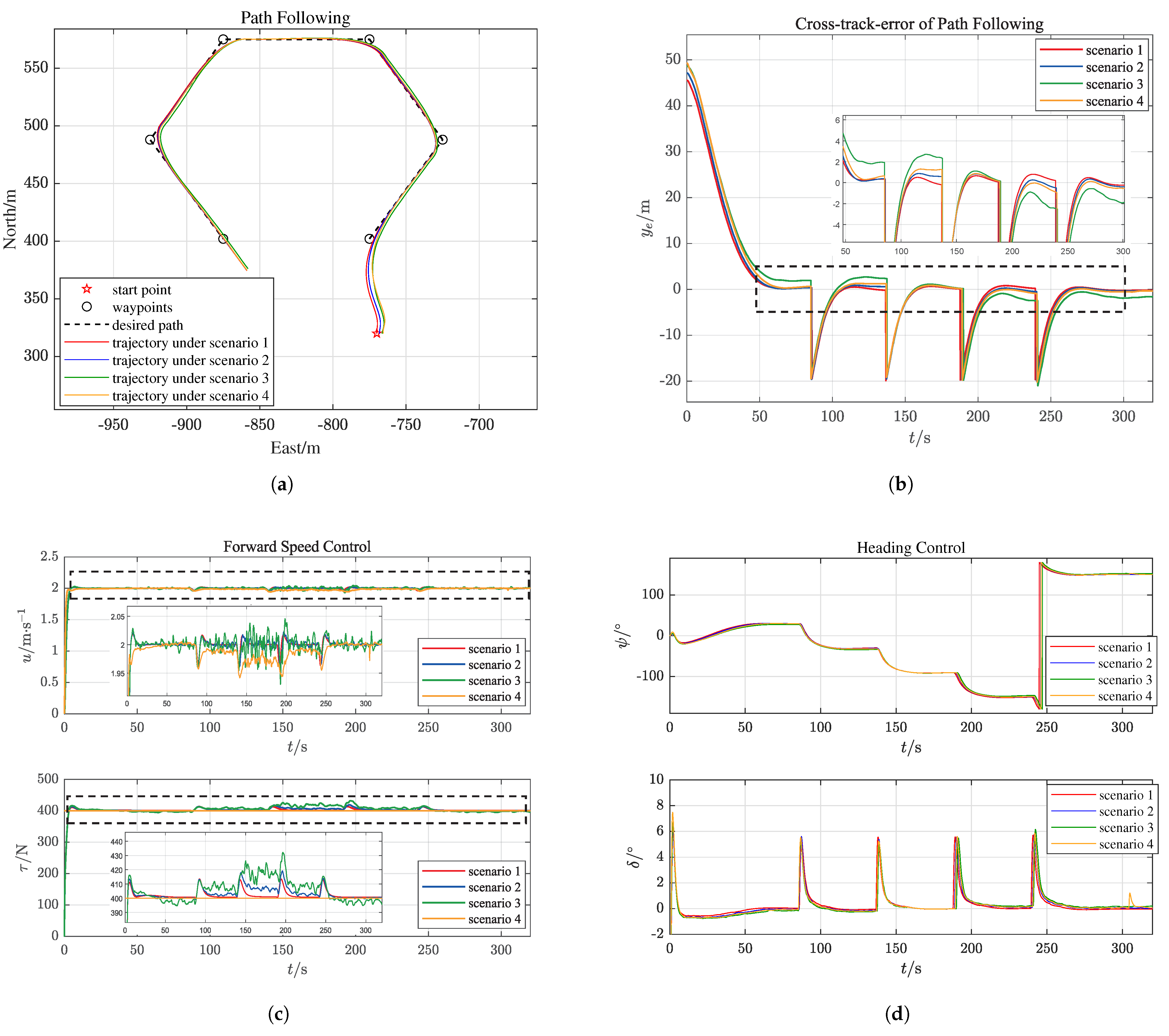
5.1.3. Path-Following Control Simulation

As shown in Figure 13, in the path-following mode, six waypoints P i ( i = 1 , 2 , , 6 ) are set, with the expected path being hexagonal and the path being P 1 - P 2 - P 3 - P 4 - P 5 - P 6 . The coordinates of each point are P 1 ( 402 , 775 ) , P 2 ( 488 , 725 ) , P 3 ( 575 , 775 ) , P 4 ( 575 , 875 ) , P 5 ( 488 , 925 ) , and P 6 ( 402 , 875 ) .
Set the initial position of the WAMV near the dock, with an initial yaw angle of 0° and a surge velocity of 0. The path-following simulation test is carried out in four scenarios as shown in Table 4.
Figure 14a shows the trajectory of the WAMV, where the dashed line represents the desired path and the solid line represents the actual trajectory. Figure 14b shows the variation curve of cross-track error. Figure 14c shows the variation curves of surge velocity and thrust. Figure 14d shows the variation curves of yaw angle and azimuth angle. In each figure, the red, blue, green, and yellow lines correspond to the four scenarios mentioned above.
In all four scenarios, the USV can smoothly and quickly track the desired path, with cross-track errors of less than 0.8 m, 0.9 m, 2.7 m, and 1.3 m, respectively; the yaw angle changes are stable without overshoot, and the azimuth angle changes steadily with a small amplitude; the overshoot of the surge velocity in scenarios (1), (2), and (3) is less than 0.9%, 1.1%, and 1.4%, respectively. The adjustment time is less than 3.8 s and there is no steady-state error. In scenario (4), the surge velocity fluctuation is less than 0.1 m/s. The results show that under the same interference conditions, the control effect of surge velocity joint control on path-following (0.9 m) is significantly better than that of surge velocity open-loop control (1.3 m).

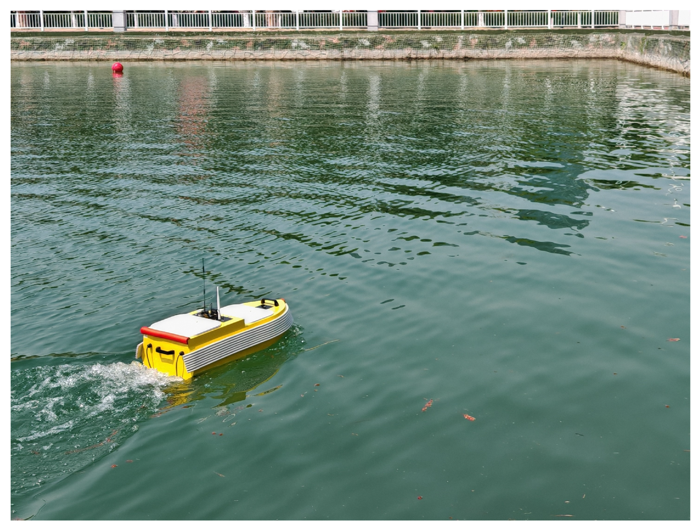
5.2. Water Tank Experiment

To validate the feasibility of rapid USV development using the proposed simulation system, the “Noah” USV developed by AMOVLab [20] was employed to conduct water tank experiments under the most comprehensive path-following mode. The experimental environment is shown in Figure 15.
As in Section 5.1.3, the waypoint coordinates were set as P1 (−20, −44), P2 (−20, −60), P3 (−33.8, −68), P4 (−47.6, −60), P5 (−47.6, −44), and P6 (−33.8, −36). The USV’s path-following trajectory and cross-track error curves are shown in Figure 16a and Figure 16b, respectively.
As observed in Figure 14a,b and Figure 16a,b, the trajectories in the simulation experiments are relatively smooth with minor cross-track errors, while trajectories in the water tank experiment exhibit slight oscillations around the desired path, with cross-track errors below 1 m. The consistency between simulation and experimental results demonstrates that the proposed simulation system effectively simulates the USV’s motion characteristics and real-world scenarios, confirming its validity for control algorithm verification.

6. Conclusions

This paper explores the design of a motion control simulation system for USVs based on the virtual USV environment VRX and Simulink. Three control modes combined with speed control were considered, including yaw rate control, heading control, and path-following control. Speed, heading, yaw rate, and path guidance controllers were designed. The simulation tests under three control modes verified that the simulation system design is successful. The feasibility of the proposed simulation system for USV rapid development was validated through path-following water tank experiments. The simulation system combines the high fidelity of VRX in real-world scenarios and the intuitive and efficient use of Simulink to design controllers, which will facilitate the rapid prototyping of new control algorithms and the preliminary validation and optimization of algorithms before actual testing. In the future, the simulation system will be expanded and various open-source ROS2 feature packages will be introduced, such as vision_opencv, Cartographer, and Navigation2, to conduct research on USV target recognition, Simultaneous Localization and Mapping (SLAM), and path planning.

Supplementary Materials

The following supporting information can be downloaded at https://www.mdpi.com/article/10.3390/app15084213/s1.

Author Contributions

Conceptualization, P.J. and W.L.; methodology, P.J. and W.L.; software, P.J. and Y.Y.; validation, W.L.; data curation, P.J., Y.Y. and C.S.; writing—original draft preparation, P.J.; writing—review and editing, P.J., W.L., Y.Y. and Y.Z.; supervision, W.L.; project administration, W.L.; funding acquisition, W.L. All authors have read and agreed to the published version of the manuscript.

Funding

This research was funded by the National Natural Science Foundation of China under grant number 42174051.

Institutional Review Board Statement

Not applicable.

Informed Consent Statement

Not applicable.

Data Availability Statement

The original contributions presented in this study are included in the Supplementary Materials. Further inquiries can be directed to the corresponding authors.

Conflicts of Interest

The authors declare no conflicts of interest.

Abbreviations

The following abbreviations are used in this manuscript:
USVUnmanned Surface Vehicle
VRXVirtual RobotX
ROSRobot Operating System
GNSSGlobal Navigation Satellite System
IMUInertial Measurement Unit
OSRFOpen Source Robotics Foundation
DDSData Distribution Service
QoSQuality of Service
WAMVWave-Adaptive Modular Vehicle
PIDProportion–Integration–Differentiation
EKFExtended Kalman Filter
UKFUnscented Kalman Filter

References

  1. Zhang, J.; Li, X.; Zhou, H.; Wu, X. Analysis and Research on Operational Application of Unmanned Surface Vehicles in Russia-Ukraine Conflict. Digit. Ocean. Underw. Warf. 2024, 7, 616–622. [Google Scholar] [CrossRef]
  2. Fan, Y.; Yang, S.; Huang, J.; Xiang, X. Design and verification of unmanned surface vehicle integrated simulation platform based on USVSim. J. Ordnance Equip. Eng. 2022, 43, 21–27. [Google Scholar] [CrossRef]
  3. Xiao, G.; Zheng, G.; Tong, C.; Hong, X. A Virtual System and Method for Autonomous Navigation Performance Testing of Unmanned Surface Vehicles. J. Mar. Sci. Eng. 2023, 11, 2058. [Google Scholar] [CrossRef]
  4. Paravisi, M.; Santos, D.H.; Jorge, V.; Heck, G.; Gonçalves, L.M.; Amory, A. Unmanned Surface Vehicle Simulator with Realistic Environmental Disturbances. Sensors 2019, 19, 1068. [Google Scholar] [CrossRef] [PubMed]
  5. Woo, J.; Lee, J.; Kim, N. Obstacle avoidance and target search of an Autonomous Surface Vehicle for 2016 Maritime RobotX challenge. In Proceedings of the 2017 IEEE Underwater Technology (UT), Busan, Republic of Korea, 21–24 February 2017; pp. 1–5. [Google Scholar] [CrossRef]
  6. Smith, P.; Dunbabin, M. High-Fidelity Autonomous Surface Vehicle Simulator for the Maritime RobotX Challenge. IEEE J. Ocean. Eng. 2019, 44, 310–319. [Google Scholar] [CrossRef]
  7. Jung, W.; Woo, J.; Kim, N. Recognition of the light buoy for scan the code mission in 2016 Maritime RobotX Challenge. In Proceedings of the 2017 IEEE Underwater Technology (UT), Busan, Republic of Korea, 21–24 February 2017; pp. 1–5. [Google Scholar] [CrossRef]
  8. Sang, X. Hands-On ROS2 for Robotics Programming: From Introduction to Practice; Machine Press: Beijing, China, 2024. [Google Scholar]
  9. Chu, Y.; Wu, Z.; Zhu, X.; Yue, Y.; Lim, E.G.; Paoletti, P.; Ma, J. Riverbank Following Planner (RBFP) for USVs Based on Point Cloud Data. Appl. Sci. 2023, 13, 11319. [Google Scholar] [CrossRef]
  10. Lu, G. Research on Path Planning and Control Method of Unmanned Vessel Based on ROS. Master’s Thesis, Hangzhou Dianzi University, Hangzhou, China, 2023. [Google Scholar]
  11. Zhang, Y.; Li, H.; Wang, Z. Design of a virtual simulation experimental platform for intelligent control of unmanned surface vehicles based on VRX. Exp. Technol. Manag. 2024, 41, 121–128. [Google Scholar] [CrossRef]
  12. Bayrak, M.; Bayram, H. COLREG-Compliant Simulation Environment for Verifying USV Motion Planning Algorithms. In Proceedings of the OCEANS 2023–Limerick, Limerick, Ireland, 5–8 June 2023; pp. 1–10. [Google Scholar] [CrossRef]
  13. Meng, J.; Humne, A.; Bucknall, R.; Englot, B.; Liu, Y. A Fully-Autonomous Framework of Unmanned Surface Vehicles in Maritime Environments Using Gaussian Process Motion Planning. IEEE J. Ocean. Eng. 2023, 48, 59–79. [Google Scholar] [CrossRef]
  14. ROS Toolbox Getting Started Guide. Available online: https://ww2.mathworks.cn/help/ros/getting-started-with-ros-toolbox.html (accessed on 17 December 2024).
  15. Fossen, T. Handbook of Marine Craft Hydrodynamics and Motion Control, 2nd ed.; Wiley: Hoboken, NJ, USA, 2021. [Google Scholar]
  16. Sarda, I.; Qu, H.; Bertaska, I.; Ellenrieder, K. Station-keeping control of an unmanned surface vehicle exposed to current and wind disturbances. Ocean. Eng. 2016, 127, 305–324. [Google Scholar] [CrossRef]
  17. Bingham, B.; Agüero, C.; McCarrin, M.; Klamo, J.; Malia, J.; Allen, K.; Lum, T.; Rawson, M.; Waqar, R. Toward Maritime Robotic Simulation in Gazebo. In Proceedings of the OCEANS 2019 MTS/IEEE SEATTLE, Seattle, WA, USA, 27–31 October 2019; pp. 1–10. [Google Scholar] [CrossRef]
  18. Moore, T.; Stouch, D. A Generalized Extended Kalman Filter Implementation for the Robot Operating System. Intell. Auton. Syst. 2016, 302, 335–348. [Google Scholar] [CrossRef]
  19. Shi, S. Submarine Maneuverability; National Defense Industry Press: Beijing, China, 1995. [Google Scholar]
  20. Tutorial for the Use of Unmanned Boats. Available online: https://amovlab.com/service (accessed on 30 March 2025).
Figure 1. Geographic and body-fixed reference frame.
Applsci 15 04213 g001
Figure 2. Thrust generated by the two podded thrusters.
Applsci 15 04213 g002
Figure 3. Schematic diagram of motion control system.
Applsci 15 04213 g003
Figure 4. Circle of acceptance.
Applsci 15 04213 g004
Figure 5. Integral line-of-sight guidance law.
Applsci 15 04213 g005
Figure 6. Schematic diagram of VRX/Simulink simulation system.
Applsci 15 04213 g006
Figure 7. Controllers and ROS2 interface modules in Simulink.
Applsci 15 04213 g007
Figure 8. ROS2 interface modules in Simulink.
Applsci 15 04213 g008
Figure 9. Modules of WAMV.
Applsci 15 04213 g009
Figure 10. Connection relationships among system nodes.
Applsci 15 04213 g010
Figure 11. The simulation result of yaw rate control. (a) Surge velocity and thrust variation curves. (b) Yaw rate and azimuth angle variation curves.
Applsci 15 04213 g011
Figure 12. The simulation result of heading control. (a) Surge velocity and thrust variation curves. (b) Yaw angle and azimuth angle variation curves.
Applsci 15 04213 g012
Figure 13. Waypoints and the desired path.
Applsci 15 04213 g013
Figure 14. Simulation result for path-following. (a) Trajectory in path-following mode. (b) Cross-track error variation curve. (c) Surge velocity and thrust variation curves. (d) Yaw angle and azimuth angle variation curves.
Applsci 15 04213 g014
Figure 15. The experimental environment.
Applsci 15 04213 g015
Figure 16. The water tank experiment result. (a) Path-following trajectory. (b) Cross-track error curves.
Applsci 15 04213 g016
Table 1. Parameters of WAMV.
NamePhysical Quantity [Unit]Value
Vessel LengthL [m]4.9
Vessel WidthB [m]2.06
Longitudinal Center of GravityLCG [m]1.4
Economic Speed U 0 [ m · s 1 ]2
Maximum Thrust T max [N]1000
No Load DraftD [m]0.2
Massm [kg]180
Moment of Inertia around the Z-axis I z [ kg · m 2 ]466
Added Mass X u ˙ [kg]−9
Y v ˙ [kg]−167
N r ˙ [ kg · m 2 ]−335
Hydrodynamic Coefficients X u [ kg · s 1 ]−100
X u | u | [ kg · m 1 ]−150
Y v [ kg · s 1 ]−100
Y v | v | [ kg · m 1 ]−100
N r [ kg · m 2 · s 1 ]−800
N r | r | [ kg · m 2 ]−800
Nomoto Model ParametersK [ s 1 ]2.308
T [s]1.724
Table 2. Device errors of IMU and GNSS.
NamePhysical Quantity [Unit]Value
Gyroscope Dynamic Bias Stability ε   [ ° · h 1 ] 4.1
Accelerometer Dynamic Bias Stability   [ μ g ] 38.3
GNSS Horizontal Position Standard Deviation v p   [ m ] 1.0
GNSS Velocity Standard Deviation v v [ m ] 0.1
Table 3. Parameters of reference models and controllers.
Parameter [Unit]ValueParameter [Unit]Value
λ u [ rad · s 1 ]1.4 ω n ψ [ rad · s 1 ]0.7
ζ u [1]1 ζ r ψ [1]1
ω n u [ rad · s 1 ]1.3 ω nr ψ [ rad · s 1 ]0.6
λ r [ rad · s 1 ]3.5 R i + 1 [m]25
ζ r [1]1 Δ / m [1]30
ω n r [ rad · s 1 ]3 κ [1]0.001
ζ ψ [1]1
Table 4. Four different scenarios.
Scenario(1)(2)(3)(4)
Wind speed03 m/s6 m/s3 m/s
Wind direction-90°90°90°
Wave gain00.510.5
Wave period-5 s5 s5 s
Average wave direction-90°90°90°
Surge velocity2 m/s2 m/s2 m/sopen-loop with T c = 200 N
Disclaimer/Publisher’s Note: The statements, opinions and data contained in all publications are solely those of the individual author(s) and contributor(s) and not of MDPI and/or the editor(s). MDPI and/or the editor(s) disclaim responsibility for any injury to people or property resulting from any ideas, methods, instructions or products referred to in the content.

