Object-Based Downscaling Method for Land Surface Temperature with High-Spatial-Resolution Multispectral Data

Abstract

Land surface temperature (LST) is an important environmental parameter in many fields. However, many studies require high-spatial- and high-temporal-resolution LST products to improve the coarse spatial resolution of moderate-resolution imaging spectroradiometer (MODIS) LSTs. Numerous approaches have downscaled MODIS LST images to a finer spatial resolution using pixel-based image analysis (PBA). Meanwhile, object-based image analysis (OBIA) methods, which have developed rapidly in the analysis of high-spatial-resolution visible and near-infrared (VNIR) band data, have received little attention in the LST downscaling field. In this paper, we propose an object-based downscaling (OBD) method for MODIS LST using high-spatial-resolution multispectral images (e.g., Landsat Thematic Mapper (TM), Enhanced Thematic Mapper Plus (ETM+), and Advanced Spaceborne Thermal Emission and Reflection Radiometer (ASTER)) as auxiliary data. The fundamental principle of this method is to preserve the thermal radiance of the “object”, which is composed of several MODIS LST pixels (partly or entirely) and is unchanged after disaggregation into subpixels in the resulting LST image. The decomposition process consists of two key parts: the thermal radiance (TR) estimation of the object from MODIS LST products and the weight calculation of sub-objects or subpixels. Objects were generated from VNIR data and remote sensing indices (e.g., the normalized difference vegetation index (NDVI), the normalized difference built-up index (NDBI), and fractions of different endmembers) using a multiscale segmentation method. The radiance of subpixels or sub-objects was calculated based on the weights of their parent objects, which were estimated by the relationships between the remote sensing indices and the LST. The accuracy and the efficiency of the OBD method were validated using a pair of ASTER and MODIS datapoints that were acquired at the same time. The decomposed LST results showed that the spatial distribution of the downscaled LST image closely resembled the true LST of the ASTER, with an RMSE of 2.5 K for the entire image. A comparison with PBA methods for pixel downscaling also indicated that the OBD method achieves the lowest root mean square error (RMSE) across different landcovers, including urban areas, water bodies, and natural terrain. Therefore, the proposed OBD method significantly enhances the capability of increasing the spatial resolution of coarse MODIS LST, providing an alternative for improving the spatial resolution of MODIS LST images and expanding their applicability to studies that require high-temporal- and high-spatial-resolution LST products.

1. Introduction

Land surface temperature (LST) products generated from a Moderate-Resolution Imaging Spectroradiometer (MODIS) are significant for various studies of surface processes, including land–air interactions [1,2], water resource management [3,4], agricultural drought [5], and environmental biogeochemistry [6], primarily due to their relatively high revisit time. However, the relatively low spatial resolution, of 1000 m, of the MODIS LST product limits its applicability in studies requiring high temporal and spatial resolutions to identify detailed variations in the thermal heat flux across the study region [7,8,9,10,11,12]. Therefore, downscaling the MODIS LST to higher spatial resolutions is crucial to meet the needs of many studies, such as argon-drought monitoring and urban heat island monitoring, which require pixel-level detail to capture LST variations in complex environments [13,14,15,16].

Downscaling involves enhancing the spatial resolution of data [17]. LST downscaling in remote sensing typically leverages the relationships between different spatial resolutions in the form of regression models to predict the LST at finer resolutions. These methods can be broadly categorized into two types: direct LST downscaling and thermal radiance (TR) downscaling [18,19,20]. Many researchers have conducted studies on direct LST downscaling methods, which typically utilize the regression relationship between the LST and remote sensing indices (RSIs) [21,22,23,24,25]. The DisTrad method is a typical approach that utilizes a linear regression relationship between the LST and the NDVI to downscale the MODIS LST to finer spatial resolutions [26]. Essa found that a regression model using only the LST and the NDVI was insufficient to capture the LST spatial distribution in urban areas and proposed an enhanced Disaggregation of Thermal Radiometry (DisTrad) method incorporating 15 remote sensing indices [27]. Zakšek and Oštir decomposed the pixels of MODIS LST images using the relationship between LST and principal components within a moving window over a high-resolution auxiliary image [28]. Gao et al. further explored the impact of varying the size of the moving window on the regression relationship between the LST and the RSI [29].

TR downscaling methods generate downscaled LSTs using the physical thermal properties of different landcovers, rather than relying directly on LST and RSI relationships [30,31,32,33,34]. Liu and Pu developed a physical method to decompose low-spatial-resolution TR for subpixel LST retrieval by employing a scale-invariant model on MODIS TR and the statistical relationship between MODIS TR and different landcover fractions using high-resolution auxiliary data [30]. Jing and Cheng downscaled MODIS TR through a nonlinear transformation to maximize the correlation between MODIS TR and various VNIR bands [35]. Wang et al. introduced a two-step pixel decomposition method that transitions from TR decomposition to LST downscaling, ensuring that the thermal radiance of parent pixels in the MODIS LST image remains unchanged [36,37]. Beyond these two categories of downscaling methods, efforts have also been made to apply artificial neural networks [38] and spectral unmixing models [39] for disaggregating Landsat TM thermal data and airborne, hyperspectral remote sensing data from the DAIS [40,41,42]. However, most existing LST downscaling methods are based on pixel-by-pixel image analysis, which has inherent limitations. Pixel-based approaches often struggle to capture spatial patterns and contextual information, particularly in heterogeneous landscapes, leading to the so-called “salt and pepper effect” [43]. These methods also fail to account for the spatial relationships between neighboring pixels, which are crucial for accurately representing land surface processes. Given these limitations, there is a need to explore alternative approaches that can better capture spatial and contextual information [15,16].

Traditional pixel-based approaches often struggle in heterogeneous landscapes, leading to the so-called “salt and pepper effect”, where spatial relationships between pixels are ignored, resulting in fragmented and contextually poor outputs [31,32]. This phenomenon occurs because pixel-based methods analyze each pixel independently, based solely on its spectral properties (e.g., reflectance or radiance values), without considering the spatial relationships or contextual information between neighboring pixels. In heterogeneous landscapes, where landcover types vary significantly over short distances, this approach fails to capture the continuity and spatial patterns of land surface features. For example, in urban areas, a single pixel might cover parts of a building, a road, and vegetation, leading to mixed spectral signatures that are difficult to interpret accurately. As a result, the output often appears as a noisy, patchy image with abrupt transitions between pixel values, resembling the scattered appearance of salt and pepper—hence the term “salt and pepper effect”. This lack of spatial coherence and contextual understanding limits the ability of pixel-based methods to accurately represent complex land surface processes, particularly in areas with high spatial variability. In contrast, OBIA not only considers the spectral properties of pixels but also integrates spatial information, such as shape, texture, and neighborhood relationships, significantly improving the ability to identify and classify complex land surface features [39]. This approach has been successfully applied in various domains, such as landcover classification [30,31], forest structure analysis [29], and damage assessment. Compared to single pixels, the “objects” generated by segmentation offer significant advantages in terms of spectral information (e.g., the statistical values per band: mean, minimum, maximum values, mean ratios, etc.) and spatial dimension information (e.g., distance, neighborhood, topologies, etc.) [44,45,46]. The OBIA method can efficiently overcome the so-called “salt and pepper effect” phenomenon, which is prevalent in traditional pixel-based image analysis [47].

Recent attention has been drawn to using high-resolution satellite imagery (e.g., IKONOS, QuickBird, Worldview) or relatively high-resolution multiscale satellite imagery (e.g., ASTER, Landsat TM) to evaluate forest land use structures [48,49], enhance the accuracy of landcover/land use information in heterogeneous areas [50,51], and assess damage caused by building collapses during earthquakes and conflicts. Despite these advances, little work has been carried out on LST downscaling using OBIA, as OBIA is traditionally an upscaling process that aggregates high-resolution pixels into relatively lower-resolution “objects”. However, by reversing the conventional OBIA process, could this approach yield improved results in LST downscaling?

The objective of this paper is to introduce the OBIA method for MODIS LST downscaling, using relatively high-spectral-resolution multispectral imagery (e.g., Landsat TM, ETM+, ASTER) as auxiliary data [39,52,53]. The key breakthrough in this study lies in the proper creation of objects and maintaining their thermal radiance after downscaling. The proposed approach involves three main steps: the initial radiance estimation of the parent object, the decomposed radiance of sub-objects, and the final temperature determination [12,54,55,56]. After outlining the theoretical principles and image processing procedures of the OBIA-based downscaling (OBD) approach, we validate its accuracy by comparing it with various pixel-based approaches (PBAs) through a designed experiment. Consequently, this paper is organized with a Section 2 presenting the details of the OBD approach, a Section 3 to validate and discuss the approach, and a Section 4 summarizing the key findings of this study.

2. Methodology

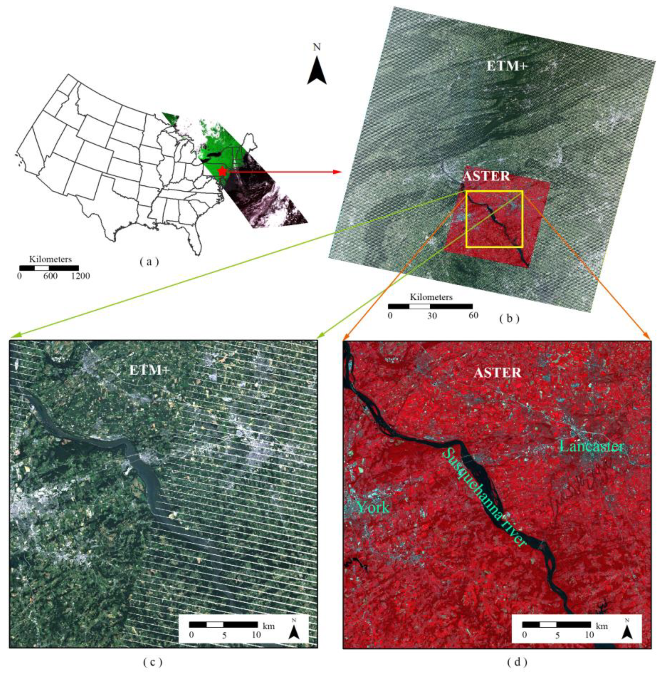
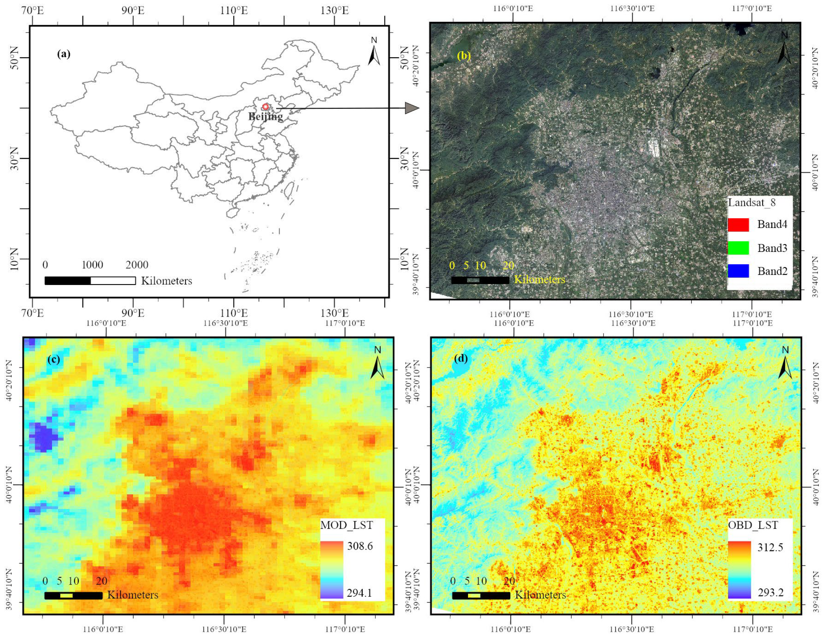
2.1. Study Area and Datasets

MODIS LST data, with an initial spatial resolution of 1000 m, were downscaled to 90 m using high-resolution land surface thermal properties derived from ASTER and Landsat ETM+ visible/infrared (VNIR) data. In this study, ASTER VNIR data assisted in the decomposition of MODIS LST pixels from 1000 m to 90 m, with ASTER-observed LSTs serving as the reference values to validate the downscaled MODIS LST results [51]. MODIS, ASTER, and Landsat ETM+ images for the Lancaster and York region were acquired on 24 August 2003. MODIS and ASTER data were captured simultaneously at 16:02:52 GMT (11:02:52 local time), while Landsat ETM+ data were acquired at 15:34:26 GMT (10:34:26 local time).

For the study area in the northeastern United States of America (USA) (Figure 1), we acquired multiple satellite products to support our thermal downscaling approach: (1) MODIS MOD11A1 land surface temperature (LST) and emissivity products as the primary coarse-resolution thermal inputs; (2) ASTER AST_08 LST (90 m) and AST_05 emissivity data for the validation; (3) ASTER AST_L1B multispectral data (15–90 m resolution across VNIR-SWIR bands) to derive spectral indices and support image segmentation; and (4) Landsat 7 ETM+ multispectral data (30 m resolution) to enhance the landcover characterization and spatial detail.

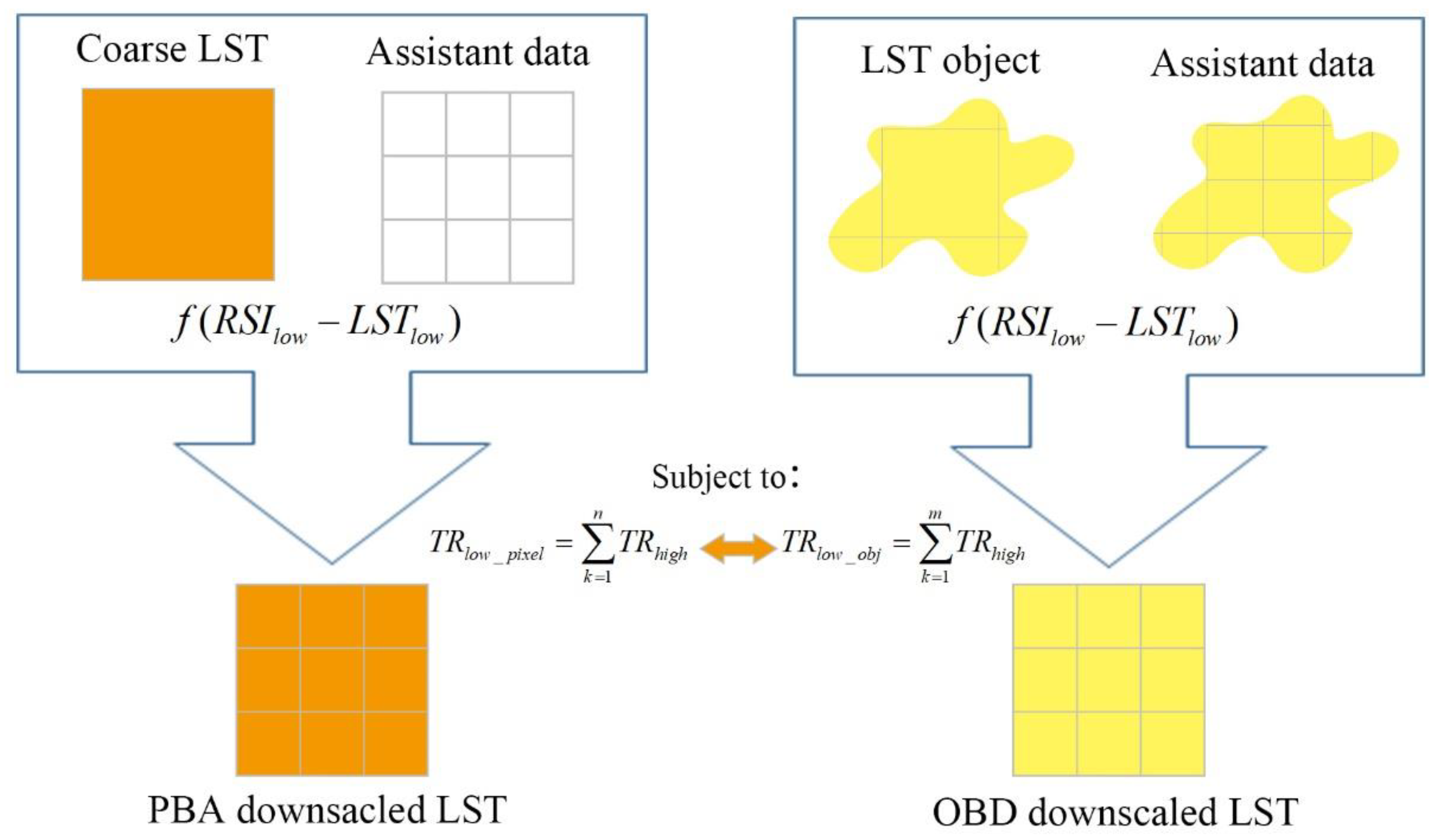
2.2. Theoretical Principle of OBD

As illustrated in Figure 2, the fundamental distinction between pixel-based (PBA) and object-based (OBD) downscaling approaches lies in their thermal property treatment during resolution enhancement. The upper section of Figure 2 demonstrates the conventional PBA methodology, which processes thermal data at the individual pixel level by establishing statistical correlations between coarse-resolution land surface temperatures and spectral indices from auxiliary datasets. In contrast, the lower schematic presents our proposed OBD framework, which implements object-oriented thermal conservation principles. Here, multiscale segmentation generates homogeneous units (labeled “LST objects” in Figure 2) that serve as fundamental thermal redistribution units. This approach maintains the physical consistency of landcover thermal characteristics through object-level radiation constraints while effectively eliminating the pixel-scale discontinuities that become apparent when comparing PBA and OBD results.

The LST retrieved from the MODIS thermal infrared band had a relatively high temporal resolution and a low spatial resolution. Many PBA downscaling approaches could be expressed as Equation (1), using the LST and RSI relationships ($f(RS{I}_{low}-LS{T}_{low})$) to downscale the MODIS LST with high-resolution VNIR data (eg: Landsat or ASTER) as assistance. LST and RSI relationships may be linear, nonlinear, or non-uniformly generated from different window sizes or whole images. Figure 2 illustrates the main process of the OBD method. Some constraints, like maintaining the TR unchanged after downscaling, as shown in Equation (2), were used.

$$LS{T}_{high}=f(RS{I}_{low}-LS{T}_{low})f(RS{I}_{high})$$

(1)

Subject to

$$T{R}_{low\_pixel}={\displaystyle \sum _{k=1}^{n}T{R}_{high}}$$

(2)

The OBD approach:

$$T{R}_{low\_obj}={\displaystyle \sum _{k=1}^{m}T{R}_{high}}$$

(3)

Enhancing the spatial resolution of MODIS land surface temperature (LST) data necessitates the incorporation of auxiliary datasets. The methodology involved comprehensive pre-processing procedures: dataset format conversion, geometric correction, the calculation of effective thermal radiance, and the derivation of essential spectral indices (including the NDVI, NDBI, and MNDWI). Subsequently, a multi-sensor fusion technique was implemented to achieve the improved LST resolution. Figure 3 illustrates the main process of the approach for LST decomposition. Mainly, two parts are involved in the process: the thermal radiance (TR) estimation of objects from MODIS LST products and the weight calculation of sub-objects or subpixels. The TR estimations of objects are determined by the region covered by the object of the MODIS TR. The objects were generated by OBIA methods with high-resolution multispectral data, and some remote sensing indices (RSIs) had fine relationships with the LST (e.g., the NDVI, the NDBI, and fractions of different endmembers). The MODIS TRs of the pixels were computed by their LST and broadband emissivity (BBE).

Finally, the TR of the objects was downscaled into a fine spatial resolution with the weights of subpixels in each object and maintain the thermal radiance of the object unchanged after it is disaggregated into the subpixels in the resulted image. The weights of the subpixels in each object were determined through the initial downscaled LSTs that were estimated by the RSI auxiliary data and the LST-RSI relationships.

2.3. Thermal Radiance Estimation of Objects

The thermal radiance of objects composed of several MODIS TR pixels was estimated in two steps: We identified the MODIS TR pixels that were totally or partly covered by the object, as shown in Figure 4, mainly because the area of the objects generated from the high-resolution multispectral data may not have exactly overlaid several MODIS pixels entirely. Then, the TR of the object (R_obj) was calculated with the MODIS pixels through Equation (4):

$$R_{\mathrm{obj}}={\displaystyle \frac{{\displaystyle \sum _{i=1}^M{R}_{\mathrm{mod},i}{S}_{\mathrm{mod}}+}{\displaystyle \sum _{j=1}^N{R}_{\mathrm{mod},j}{S}_{\mathrm{mod}}{W}_j}}{S_{\mathrm{obj}}}}$$

(4)

where $R_{\mathrm{mod},i}$ is the TR of the MODIS pixel, i, that is totally covered by the object; $S_{\mathrm{mod}}$ is the area of the MODIS pixel, i, that is totally covered by the object; M is the number of MODIS pixels that are totally covered by the object; $R_{\mathrm{mod},j}$ is the TR of the MODIS pixel, j, that is partly covered by the object; N is the number of MODIS pixels that are partly covered by the object; $W_j$ is the weight of the MODIS TR pixels that are partly covered by the object; and $S_{\mathrm{obj}}$ is the area of the object.

The thermal radiance conservation condition is expressed by Equation (5):

$${\displaystyle \sum _{j=1}^n{W}_j=1}$$

(5)

where $W_j$ are the weights of the MODIS TR pixels that are partly covered by different objects, and n is the number of parts that are decomposed by different objects.

The weight of the MODIS TR pixels that are partly covered by the object is needed for the computation of thermal radiance for each subpixel in the decomposed LST image. Wang et al. [38] gave the weight calculation method based on the initial decomposed LST that is first estimated by the assistant high-spatial-resolution data. If the initial decomposed temperature $(T_{ini\_k})$ and emissivity (${\epsilon }_{ini\_k}$) for each subpixel of the decomposed LST image at the finer resolution could be estimated, the TR of each subpixel at a given wavelength could calculated by the Planck equation formula for radiance through Equation (6):

$$R_{\mathrm{i}ni\_k}={\epsilon }_{ini\_k}{R}_b(T_{ini\_k})={\displaystyle \frac{{\epsilon }_{ini\_k}{K}_1}{\exp (K_2/T_{ini\_k})-1}}$$

(6)

where $R_{ini\_k}$ is the estimated TR for subpixel k, and T_{ini_k} and ε_{ini_k} are the estimated initial LST and emissivity of the subpixel k. Then, the total thermal radiance of the partly covered MODIS TR and its parts can be estimated from the pixels that are partly or totally covered by the target object through Equation (7):

$$R_{tot}={\displaystyle \sum _{k=1}^m{R}_k{S}_{tar}/S_{\mathrm{mod}}}$$

(7)

$$R_p={\displaystyle \sum _{k=1}^n{R}_k{S}_{tar}/S_p}$$

(8)

where $R_{tot}$ is the total thermal radiance of the MODIS TR for partly covered pixels, $S_{tar}$ is the area of decomposed pixels at the target resolution, m is the number of pixels decomposed from the MODIS TR at the target resolution, $R_p$ is the thermal radiance of partly covered pixels for the MODIS TR, and n is the number of pixels decomposed from the part at the target resolution, as shown in Equation (9) below:

$$W_j=R_p/R_{tot}=S_{\mathrm{mod}}{\displaystyle \sum _{k=1}^n{R}_k}/S_p{\displaystyle \sum _{k=1}^m{R}_k}$$

(9)

Therefore, we should obtain the objects and the estimated initial temperature and emissivity of subpixels at the target resolution to estimate the thermal radiance of the objects.

2.4. Objects Generated from the High-Resolution Multispectral Data

Objects are generated by image segmentation, which is the subdivision of an image into separate regions [57,58,59]. We will use the multi-resolution segmentation (MRS) method [60,61], implemented in the eCognition software 10.1, to obtain the image objects composed of grouped pixels. MRS is a clustering procedure, and smaller image objects are merged into bigger ones. The underlying optimization procedure minimizes the weighted heterogeneity. Heterogeneity, in eCognition, is considered as a primary object that features color and shape. The increase in heterogeneity, f, should be less than a certain threshold. The specific calculations are shown in Equations (10) and (11):

$$f=w_{\mathrm{color}}·\Delta h_{\mathrm{color}}+w_{\mathrm{shape}}·\Delta h_{\mathrm{shape}}$$

(10)

Subject to:

$$w_{\mathrm{color}}+w_{\mathrm{shape}}=1,w_{\mathrm{color}}\in [0,1],w_{\mathrm{shape}}\in [0,1]$$

(11)

The weight parameters (w_color, w_shape) allow us to adapt the heterogeneity definition to the application. The spectral heterogeneity, $\Delta h_{\mathrm{color}}$, allows for multi-variant segmentation to different image channels. The shape heterogeneity, $\Delta h_{\mathrm{shape}}$, is a value that describes the improvement of the shape with regard to the smoothness and compactness of an object’s shape.

The scale parameter is the stop criterion for the optimization process. Prior to the fusion of two adjacent objects, the resulting increase in heterogeneity is calculated. If this resulting increase exceeds a threshold value determined by the scale parameter, then no further fusion takes place and the segmentation stops. The larger the scale parameter, the more objects can be fused and the larger the objects grow. Since one MODIS LST pixel (1000 m) covers more than 120 ASTER LST pixels (90 m), the level 1 scale was chosen as 200 to make the area of the segmentation object larger than one MODIS LST at this level. While the object segmented at level 1 was composed of different landcovers, we chose the scale of 20 to obtain the child object for level 1. Each object, at level 2, can be classified as one landcover category (e.g., water, vegetation, soil, building) with relatively similar spectral information. Level 3 generates the smallest object, and its purpose is to identify the small difference in the spectral data of the object at level 2.

2.5. Initial LST Estimated by High-Resolution Multispectral Data

The land surface temperature (LST) of subpixels in finer resolutions represents the ultimate outcome of our downscaling efforts. Consequently, it is necessary to employ alternative methods to estimate the LST for the computation of weights for sub-objects or subpixels; the estimated LST at this stage, as the initial downscaled LST for the subpixels, is well established by surface structures, which shape the thermal performance of the ground surface. Remote sensing indices (RSIs) derived from high-spatial-resolution visible and near-infrared (VNIR) data can effectively reflect the spatial distribution of the LST. Utilizing VNIR data from ASTER and ETM+, some typical RSIs, such as the normalized difference vegetation index (NDVI), vegetation fraction (f_v), normalized difference built-up index (NDBI), impervious surface area (ISA), and fractions of endmembers (F_i), were used to estimate the initial temperature for the subpixels. The primary regression relationships between LST and RSIs are presented in

Table 1. Some LST downscaling method with VNIR data as assistance.

RSI	RSI Calculation	LST-RSI Relationship	Studies
NDVI	$NDVI={\displaystyle \frac{{\rho }_{\mathrm{NIR}}-{\rho }_{\mathrm{RED}}}{{\rho }_{\mathrm{NIR}}+{\rho }_{\mathrm{RED}}}}$	$LST={\mathrm{a}}_{1}NDVI+{\mathrm{b}}_1$	Kustas et al. [26]; Zhan et al. [11]
fv	$f_v=1-{({\displaystyle \frac{NDV{I}_{\max }-NDVI}{NDV{I}_{\max }-NDV{I}_{\min }}})}^{0.625}$	$LST={\mathrm{a}}_{2}fv+{\mathrm{b}}_2$	Agam et al. [10]
NDBI	$NDVI={\displaystyle \frac{{\rho }_{\mathrm{SWIR}}-{\rho }_{\mathrm{NIR}}}{{\rho }_{\mathrm{SWIR}}+{\rho }_{\mathrm{NIR}}}}$	$LST={\mathrm{a}}_{3}NDBI+{\mathrm{b}}_3$	Essa et al. [9]; Wang et al. [36]
ISA	$ISA=F_{\mathrm{high}\_\mathrm{albedo}}+F_{\mathrm{low}\_\mathrm{albedo}}$	$LST={\mathrm{a}}_{4}ISA+{\mathrm{b}}_4$	Essa et al. [9]
Fi	${\rho }_b={\displaystyle \sum _{i=1}^N{f}_i{\rho }_{i,b}}+e_b$ Subject to: ${\displaystyle \sum _{i=1}^N{f}_i=1}$ and $f_i\ge 0$	$LST={\displaystyle \sum _{i=1}^n{F}_i{T}_i+e}$	Deng and Wu [7]

. While individual RSIs can perform effectively within specific landcover types, it is essential to combine their indices across different landcover scenarios.

${\rho }_{\mathrm{RED}}$, ${\rho }_{\mathrm{NIR}}$ and ${\rho }_{\mathrm{SWIR}}$ are, respectively, the reflectance of the red band, near-infrared band, and the short wave infrared band; $F_{\mathrm{high}\_\mathrm{albedo}}$ and $F_{\mathrm{low}\_\mathrm{albedo}}$ are the fraction of the high albedo and the low albedo endmember in a pixel. T_i is the LST of endmember i. ${\rho }_{i,b}$ is the reflectance of endmember i in band b, and $e_b$ is the model residual.

For the natural surface covered by some vegetation, we identified that the NDVI, f_v, and F_i had a good relationship with the LST. So, an average of the LST, as estimated by the three indices, could obtain the initial decomposed LST.

$$LS{T}_{\mathrm{ini}}=\mathrm{Average}\left(f\right(NDVI),f\left(f_v),f\right(F_i\left)\right)$$

(12)

For the urban areas and surfaces with less vegetation, we identified that the NDBI, ISA, and F_i had a good relationship with the LST. So, the average of the LST, as estimated by the three indices, can generate the initial decomposed LST.

$$LS{T}_{\mathrm{ini}}=\mathrm{Average}\left(f\right(NDBI),f\left(ISA),f\right(F_i\left)\right)$$

(13)

Since the LST of a water body in an ETM+ or ASTER image may not change more than 1 K, a constant value obtained from the MODIS water body’s LST for the water body was chosen for the initial decomposed LST in the finer scales.

The relationship between the MODIS LST and the RSI could be calculated by MODIS VNIR/SWIR data, or the temperature of different endmembers could be estimated through the LST and RSI feature space. Then, the LST-RSI relationship was used alongside the high-spatial-resolution ETM+ or ASTER assistant data to obtain the initial temperature for the subpixels.

2.6. BBE Estimated by Different Thermal Infrared Bands

Th emissivity of the land surface is mainly determined by its thermo-physical characteristics. Since different satellites may have different thermal infrared band widths, it is better to integrate the narrow thermal infrared band emissivity into broad band emissivity (BBE) with different satellite products. Then, the TR of the MODIS LST is calculated by its BBE; the ASTER and the ETM+ should also estimate their BBE in the same wavelength. The BBE estimation methods of the ASTER and ETM+ are different because the ASTER has five thermal bands, and the ETM+ has only one thermal band.

Cheng et al. [8] gave the BBE estimation method of the MODIS and the ASTER with their narrow thermal band emissivity.

$${\epsilon }_{bb\_mod}=0.095+0.329{\epsilon }_{29}+0.572{\epsilon }_{31}$$

(14)

$${\epsilon }_{bb\_ast}=0.197+0.025{\epsilon }_{10}+0.057{\epsilon }_{11}+0.237{\epsilon }_{12}+0.333{\epsilon }_{13}+0.146{\epsilon }_{14}$$

(15)

where ${\epsilon }_{bb\_mod}$ is the BBE of the MODIS, and ${\epsilon }_{29}$ and ${\epsilon }_{31}$ are, respectively, MODIS thermal band emissivity values of 29 and 31 from the MODIS emissivity product (MOD11A1). ${\epsilon }_{bb\_ast}$ is the BBE of the ASTER, and ${\epsilon }_{10}$ to ${\epsilon }_{14}$ are the ASTER thermal narrowband emissivity values from the ASTER emissivity product (AST_05).

Li et al. [2] made an overview about the emissivity retrieval method and gave a method to estimate the emissivity using a flat pixel composed of N endmembers with a given spectral domain, as follows:

$${\epsilon }_{bb\_ETM}={\displaystyle \sum _{k=1}^N{F}_i}{\epsilon }_{endmenber,k}$$

(16)

where ${\epsilon }_{bb\_ETM}$ is the BBE of ETM+, F_i is the fraction of the endmember in a pixel, and ${\epsilon }_{endmenber,k}$ is the BBE of the typical endmembers given in

Table 2. BBE for different landcover.

Landcover	Grass	Tree	Soil	Building	Water
BBE	0.982	0.983	0.928	0.942	0.991

[46].

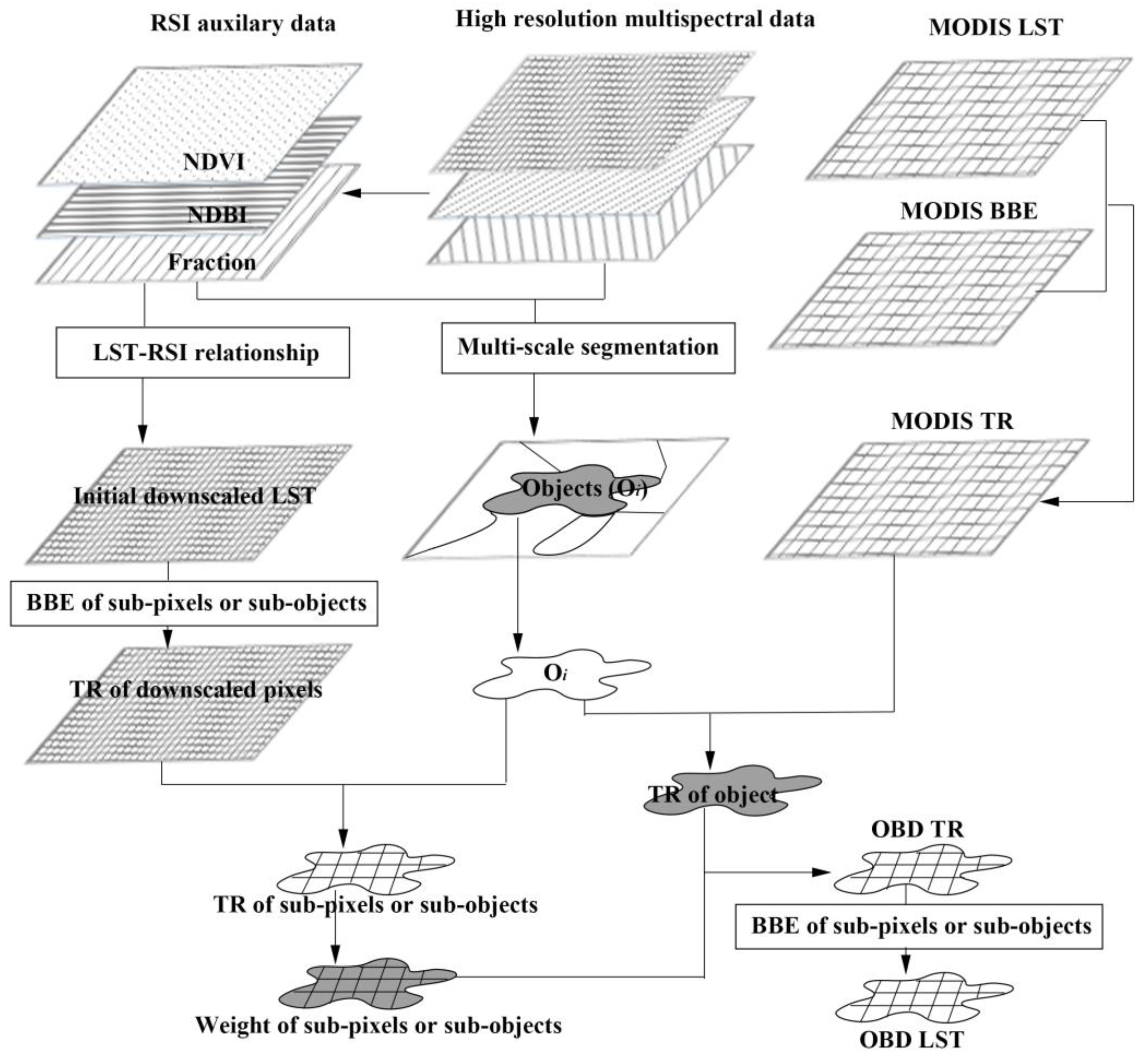
2.7. Estimation of LST in High Spatial Resolution

The weight of each subpixel or sub-object can be calculated by Equation (6) with the estimated initial temperature and BBE. Then, the downscaled TR of the subpixels or sub-objects can be easily computed as follows:

$$R_d=\left\{\begin{array}{l}{W}_k{R}_{\mathrm{obj}} \mathrm{for} \mathrm{sub}-\mathrm{pixel}\\ W_{\mathrm{sub}\_\mathrm{obj},i}{R}_{\mathrm{obj}} \mathrm{for} \mathrm{sub}-\mathrm{object}\end{array}\right.$$

(17)

where $R_d$ is the TR of subpixel $k$ or sub-object i; $W_k$ is the weight of the subpixel, $k$; $W_{\mathrm{sub}\_\mathrm{obj},i}$ is the weight of the subpixel, $i$; and $R_{\mathrm{obj}}$ is the thermal radiance of the object.

The TR of the sub-object can still be downscaled to the pixel scale in high resolution with the same process. Then, the LST of each subpixel or sub-object in the downscaling LST image can then be computed as follows:

$$T_{d\_k}={\displaystyle \frac{K_2}{\ln (1+{\epsilon }_k{K}_1/R_{d\_k})}}$$

(18)

where $T_{d\_k}$ is the decomposed LST for the subpixel, k, in the decomposed LST image.

2.8. Validation of the Approach

The best way to validate the LST downscaled results may be via comparison with a simultaneously measured LST in the same geographical region. Sometimes, the measured LST data are rarely acquired, and LST observational equipment with a high accuracy is usually expensive. So, a pair of ASTER and MODIS images matching precisely the acquisition time and place could be used as an alternative. An ASTER LST product was chosen as the true value to validate the downscaling LST image in the case that we were able to find a pair of ASTER and MODIS images matching precisely the acquisition time and place. Therefore, the downscaled MODIS LST image was to the same pixel scale as the ASTER LST image, with the ASTER and ETM+ data being used as an assistance to check the accuracy of the approach, which could be assessed through the root mean error (ME), standard deviation (SD), and root mean square error (RMSE) between the ASTER LST and the decomposed LST:

$$\mathrm{ME}={\displaystyle \sum (LS{T}_m-LS{T}_a)/N}$$

(19)

$$\mathrm{SD}=\sqrt{{\displaystyle \sum {(LS{T}_m-LS{T}_a-ME)}^2/N}}$$

(20)

$$\mathrm{RMSE}=\sqrt{{\displaystyle \sum {(LS{T}_m-LS{T}_a)}^2/N}}$$

(21)

where $LS{T}_m$ and $LS{T}_a$ are the downscaled $LST$ and the ASTER LST, respectively, for the corresponding pixels in the scale of 90 m. N is the pixel number of the ASTER LST image.

3. Results and Discussion

3.1. Downscaling of MODIS LST with ASTER and ETM+ VNIR Data

Following the downscaling procedure outlined in Figure 3, the MODIS LST product was successfully downscaled to a 90 m pixel scale using the ASTER and ETM+ VNIR data. Figure 5(a1,a2) illustrates the LST obtained from the ASTER LST product and the corresponding downscaled result from the MODIS LST product using the ASTER VNIR data. Both images display high LSTs in urban areas and lower LSTs in the suburban regions of York and Lancaster. This similar LST distribution suggests that the downscaled LST from the coarser MODIS LST image is applicable. Simultaneously, the MODIS LST product was downscaled to 90 m using the ETM+ VNIR data, given that the Landsat series represents the world’s longest continuously acquired remote sensing data collection and is freely accessible. If the OBD downscaled result proves accurate, this method could be used to generate high-spatial-resolution and high-temporal-resolution thermal remote sensing datasets utilizing MODIS and Landsat series data. The downscaled results were validated through a comparative analysis with the ASTER LST product, rather than the ETM+ LST product, due to the temporal discrepancy between the MODIS and ETM+ imaging times.

Figure 5(b1–b3) present the OBD results in a complex region containing urban areas, large rivers, and forests. Similar distributions are observed between the OBD downscaled result (Figure 5(b3)) and the ASTER LST product (Figure 5(b2)) across the entire image. However, the decomposed LST in the Susquehanna River appears more uniform in Figure 5(b3), while the true LST product shows higher LST fragments near the riverside. Figure 5(c1–c3) display the OBD results for urban and suburban areas, demonstrating similar color distributions and locations of high- and low-LST areas, indicating that the OBD method is suitable for these environments. To evaluate the similarity between the OBD downscaled results and the ASTER LST product, a scatter plot and a statistical chart were generated, as shown in Figure 6. Figure 6a presents the overall comparison scatter plot of the OBD and ASTER LST products, revealing a fitted line slope of 0.76, which is very close to a 1:1 line. Furthermore, the red area in the scatter plot is concentrated along the 1:1 line, indicating that many of the OBD results closely align with the ASTER LST product. This finding is further supported by the LST error statistics between the OBD LST and ASTER LST presented in Figure 6b. Figure 6b is the statistics plot of the OBD LST result minus the ASTER LST product. Most pixels fall within an LST error range of [0, 1] K. Approximately 80% of the total pixels demonstrate the OBD LST error within ±3 K.

To demonstrate the accuracy of the approach,

Table 3. Comparison of LST error statistics indices for different decomposition methods.

Cases		OBD Method			PBA Method
		ME	STD	RMSE	ME	STD	RMSE
ASTER	Natural terrain	−0.96	2.94	2.12	3.13	3.34	2.48
	Urban surface	−1.94	2.54	3.59	3.27	2.35	4.15
	Water bodies	−1.08	1.12	0.31	1.32	0.94	3.04
ETM+ B	Natural terrain	−1.34	2.99	2.31	−4.28	3.05	2.66
	Urban surface	−0.86	2.44	4.13	2.14	2.35	5.15
	Water bodies	0.14	0.64	0.36	−1.28	0.62	2.08
ETM+ C	Natural terrain	−1.16	2.74	2.57	−2.52	2.98	3.06
	Urban surface	0.84	3.55	3.39	3.08	3.35	3.88
	Water bodies	−0.48	0.55	0.91	1.22	0.54	1.84

Note: Geographic location of areas B and C is shown in Figure 5(a1).

presents a comparison of the downscaled LST errors between the OBD and PBA methods across different landcover types in various areas. For the entire image in the ASTER natural terrain, the mean error (ME) of the OBD method is −0.96 K, indicating that the decomposition result is, on average, 0.96 K lower than the true LST. The RMSE is 2.12 K, indicating an average error of 2.12 K in the decomposition, despite its general applicability. In comparison, the ME and RMSE of the PBA method are higher, with values of 3.13 K and 2.48 K, respectively. In region B, the predominant landscape is characterized by natural surfaces, such as vegetation, with fewer artificial surfaces, like urban areas, and a river flowing through the region. The PBA method yields a lower overall ME value for the vegetation area, reduced by 4.28 K, due to the high NDVI and vegetation component F_i values in this region. Subsequent calculations using the OBD method led to a decrease in the ME to 1.34 K, with the ME increased by 2.94 K. In urban areas, the high NDBI and impermeable component values contributed to an overall ME that is 2.14 K higher. After recalculating with the OBD method, the ME decreased to 0.86 K, with the ME increased by 1.26 K. Additionally, the ME value in water bodies increased from 1.32 K to 1.08 K. In region C, the predominant landscape is characterized by natural surfaces, such as vegetation, with much more artificial surfaces, like urban areas, than region B, and few water bodies. The PBA method yields a lower overall ME value for the vegetation area, reduced by 2.52 K, due to the high NDVI and vegetation component F_i values. Subsequent calculations using the OBD method led to a decrease in the ME to 1.16 K with the ME increased by 1.36 K. In urban areas, the high NDBI and impermeable component values contributed to an overall ME that is 3.08 K higher. After recalculating with the OBD method, the ME decreased to 0.84 K, with the ME increased by 2.22 K. Additionally, the ME value in water bodies increased from 1.22 K to 0.48 K. As shown in Table 3, the ME and the RMSE of the OBD method are consistently lower than those of the PBA method across all the landcover types, including natural terrain, urban surfaces, and water bodies. Notably, the OBD method shows a significant improvement in ME. This improvement is primarily attributed to the principle of maintaining thermal radiance unchanged after decomposition, which reduces the uncertainty of LST changes when using the NDVI, the NDBI, and other remote sensing indices (RSIs) to estimate the PBA temperature for the subpixels. At the same time, the improvement effect on the STD is relatively small. This is primarily because the weights of the subpixels within the same object are derived from the initial temperature calculations. A significant estimation error in the initial temperature will consequently lead to a substantial estimation error in the weights.

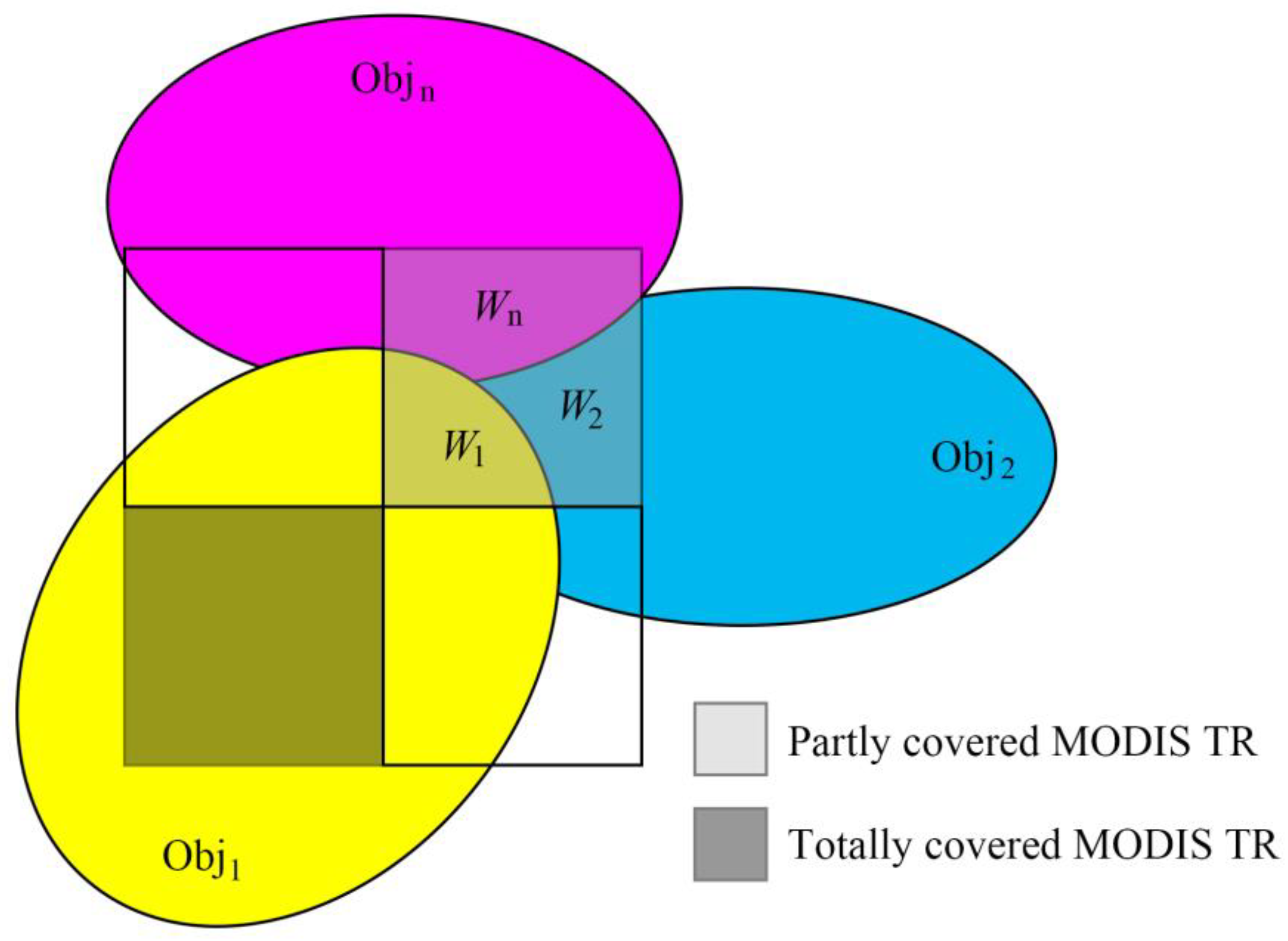
3.2. The Influence of the Object’s Weight in the OBD Method

The object-based downscaling (OBD) method effectively mitigates the salt and pepper effect associated with the initial segmentation of land surface temperature (LST) in the Pixel-Based Analysis (PBA) method and resolves the issue of energy non-conservation after downscaling. As illustrated in Figure 7, the red ellipses highlight typical urban surface types. Within these areas, the LST obtained from the PBA downscaling method is closely linked to remote sensing indices (RSIs) with an obvious “salt and pepper effect”. Following the adjustment of weights for various segmentation objects in regions U1–U6, the spatial distribution characteristics of the downscaled LST using OBD were significantly more aligned with the true temperature values observed by ASTER, and the “salt and pepper effect” of PBA disappeared. The average radiance value calculated for the region enclosed by the red ellipse is 176.5 Wm⁻². In contrast, the average radiance calculated for the PBA segmented LST in the same area is 168.5 Wm⁻², while the average for the OBD segmented LST is 174.2 Wm⁻². The green ellipse area indicates a mixed region comprising vegetation and urban areas, where the PBA exhibits a noticeable underestimation of the LST in vegetated regions and an overestimation in urban areas. After recalculating using the OBD method with the weight of V1, the previously underestimated vegetation areas were significantly elevated, while the overestimated urban building areas were mitigated. Nevertheless, compared to the true values from the ASTER, there remained an estimation error of over 2 K in this region. These findings demonstrate that the OBD method effectively addresses the overestimations and underestimations inherent in the PBA method, imposing meaningful constraints on the initially decomposed temperature values through a secondary decomposition process.

3.3. A Discussion of the Influential Elements on the OBD Results

Although we can obtain a well-decomposed LST result from the OBD method, the elements determining the accuracy of the decomposed result should be analyzed. The radiance of the object and the weight of the subpixels or sub-objects are two main influential elements of the OBD method.

The radiance error of an object is often due to the partial coverage of MODIS pixels by the edge areas of objects. If an LST image ranges between 300 K and 310 K, the radiance in the broadband would be approximately 164 Wm⁻² to 190 Wm⁻², under the assumption of a broadband emissivity (BBE) value of one. We hypothesize that the radiance errors of objects fall within the range of ±5 Wm⁻² and ±5%. Figure 8 illustrates the OBD LST error under different LST values with varying radiance errors. As shown in Figure 8a,b, the OBD LST error increases with the increasing radiance error. Additionally, the LST error varies depending on the LST value under the same radiance error. For instance, if the radiance error of an object is −4 Wm⁻², the LST error for a pixel with a true LST of 292 K ranges from −2.3 K to −1.7 K. Conversely, the LST error for a pixel with a true LST of 320 K ranges from −1.7 K to −1.1 K. The OBD LST error increases with the rising LST under a constant radiance error, as shown in Figure 8a. In contrast, the OBD LST error decreases with the rising LST under a constant radiance percentage error, as shown in Figure 8b. This occurs because higher LST values correspond to higher thermal radiance, resulting in greater radiance errors under the same percentage of radiance error.

The initial LST estimation errors, influenced by the LST-RSI relationship, primarily affect the radiance of the object and the weighting of subpixels or sub-objects. Different land surface types may exhibit similar spectral characteristics in remote sensing images, despite having significantly different temperature values. To evaluate whether our OBD method improves the decomposed results compared to the initial LST, we hypothesize that an object, represented by high-spatial-resolution multispectral remote sensing data, consists of 5000 subpixels, with temperatures ranging from 290 K to 310 K. The initial LST errors for these subpixels were randomly generated within the ranges of ±1 K, −4 to 0 K, and 0 to 4 K. We compared the mean error (ME), standard deviation (STD), and root mean square error (RMSE) between the initial LST errors and the OBD LST errors. This process was repeated 10,000 times to generate the comparative figures shown in Figure 9. Figure 9(a1–a3) presents the ME comparisons for the object under different initial LST error ranges. As shown in Figure 9(a1), the ME of the initial LST error within the ±1 K range was reduced from ±0.6 K to ±0.1 K after applying the OBD method. In Figure 9(a2,a3), the initial LST ME for the ranges of −4 to 0 K and 0 to 4 K, representing low and high LST estimates, respectively, were significantly reduced to ±0.1 K after applying the OBD method. The OBD method effectively reduces the ME, thereby preventing extreme LST estimations for subpixels. Figure 9(b1–b3) demonstrate that the OBD method does not significantly affect the STD of LST errors. However, as shown in Figure 9(c1–c3), the RMSE of the initial LST errors in the ranges of −4 to 0 K and 0 to 4 K was markedly reduced, indicating that the OBD downscaled LST results are much closer to the true LST.

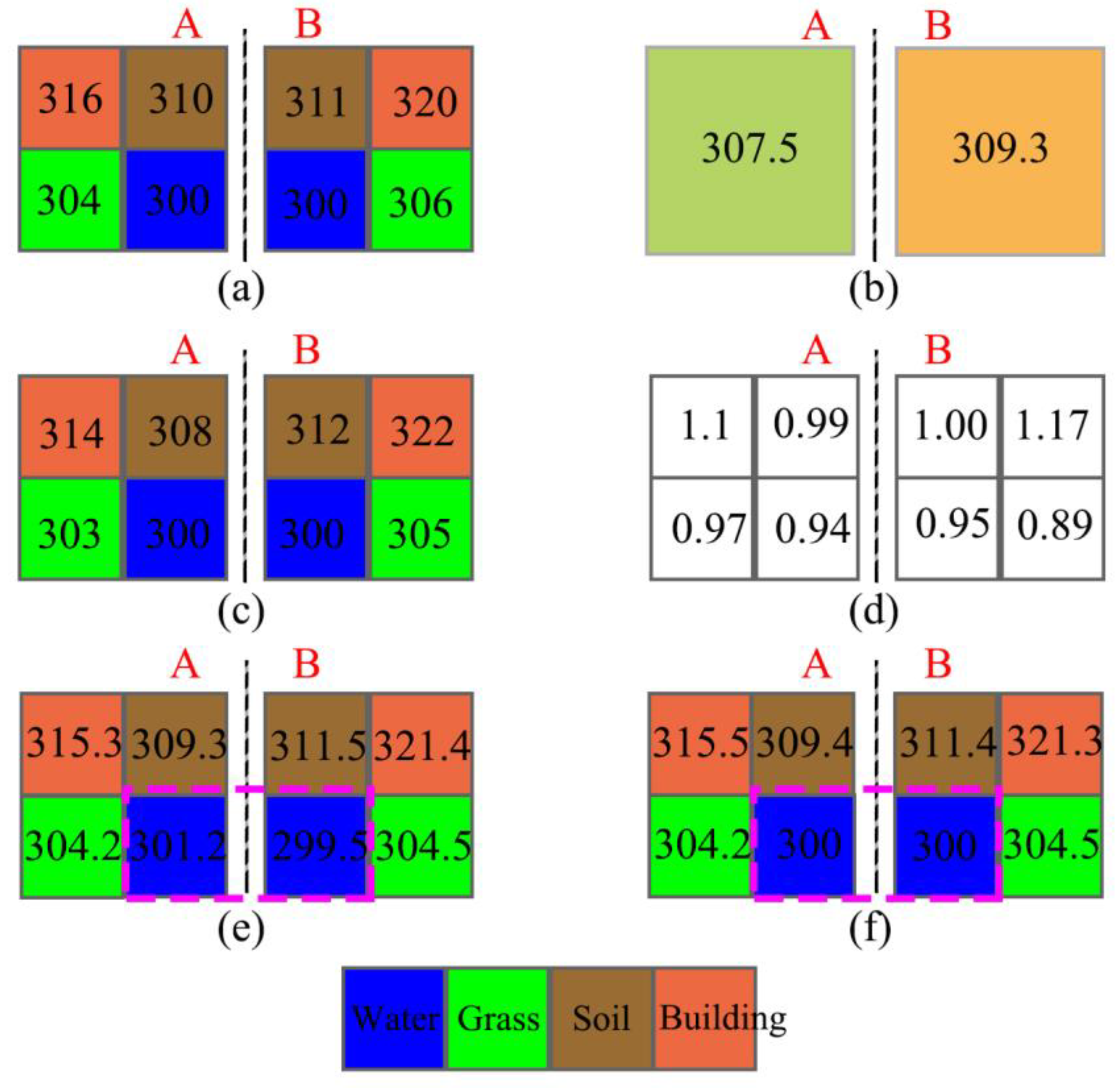
3.4. A Discussion of the Adjacency Effect in LST Downscaling

The LST and remote sensing indices’ relationships are used in most LST downscaling methods frequently. While the LST relationships of adjacent pixels have received limited attention, the OBD method could introduce the relationship of adjacent pixels in the downscaling process.

Figure 10 illustrates the process and results of applying the OBD method while considering adjacent pixels with the same land use type; in different objects, it should exhibit similar decomposed LST values. Figure 10a depicts two objects, A and B, each containing four subpixels with distinct true LST values. Figure 10b represents the true LST of the parent pixels at a lower spatial resolution, corresponding to the subpixels in Figure 10a. Figure 10c shows the initially estimated decomposed LST based on a hypothetical LST-RSI relationship, while Figure 10d presents the weights of each subpixel, calculated from this initial estimate. If only the principle of energy conservation during decomposition is considered, the results are as shown in Figure 10e. An imperfect result is observed in the pink rectangle in Figure 10e, where the decomposed LST difference between two adjacent water pixels reaches 1.7 K. Such a discrepancy is unrealistic in most natural environments. To address this, the rule specifying that the decomposed LST of adjacent water pixels across different objects should be consistent should be introduced. The decomposed LST results, considering the adjacency effect, are shown in Figure 10f. The LST difference between the adjacent water pixels in the pink rectangle is significantly reduced, resulting in a more realistic distribution. Additionally, the decomposed LST values for all the subpixels in Figure 10f are closer to the true LST values compared to those in Figure 10c,e. Thus, incorporating the adjacency effect of different objects effectively enhances the accuracy of the decomposed results.

3.5. Discussion on Applicability in Other Regions

Using MODIS and Landsat 8 imagery, captured on 30 August 2024, as experimental data; we analyzed the study area, located in Beijing, China (Figure 11a). A color composite image of the study area (Figure 11b) revealed a densely built-up central region surrounded by natural surfaces and water bodies, indicative of diverse landcover types. Figure 11c highlights a pronounced urban heat island effect, with the central urban region exhibiting surface temperatures significantly higher than the surrounding areas, with a temperature difference exceeding 10 K. By employing the OBD-based LST downscaling method, we enhanced the spatial resolution of the MODIS temperature data to match that of the Landsat multispectral data (Figure 11d). The downscaling process increased the maximum temperature values by nearly 4 K, unveiling finer details in surface temperature and enabling a clearer depiction of spatial temperature variations within urban areas. These improvements provide valuable insights for urban managers to better guide activities in zones affected by extreme temperatures.

4. Conclusions

An efficient approach has been proposed in this study to enhance the spatial resolution of MODIS LST products. The object-based downscaling (OBD) method was introduced in the LST downscaling process for MODIS LST, using high-resolution multispectral images (e.g., Landsat TM, ETM+, ASTER) as ancillary data. A unique feature of this approach is the preservation of the thermal radiance of the “object”, composed of several MODIS LST pixels, even after disaggregation into subpixels in the resultant image. The decomposition process primarily involves two critical components: the estimation of thermal radiance (TR) from MODIS LST products and the calculation of weights for sub-objects or subpixels. These objects are generated using VNIR data and various remote sensing indices (e.g., the NDVI, the NDBI, and fractions of different endmembers) through a multiscale segmentation method. The radiance of subpixels or sub-objects is calculated based on their weights within the parent objects, which are estimated using the relationships between remote sensing indices and the LST.

A series of procedures were developed for this pixel decomposition approach, including multi-resolution segmentation (MRS), which was implemented in the eCognition 10.1 software to create image objects by grouping pixels, establishing relationships between the LST and the RSI surface patterns, computing the weights for each subpixel, and determining the final temperature for the subpixels. The comparison results demonstrate that the OBD approach outperforms the PBA method, as indicated by lower ME and RMSE values across natural terrain, urban surfaces, and water bodies. The analysis reveals that two main factors—the radiance of the object and the weights of the subpixels or sub-objects—are crucial in the OBD method. Radiance errors often arise from cases where objects do not fully cover the MODIS pixel, and these errors increase with higher LST values under consistent radiance errors. The simulation of weight estimation errors for subpixels or sub-objects further confirms that the OBD method can improve the ME and the RMSE compared to the PBA method. The weight of the subpixels within the same object derived from the initial LST calculations is the most important factor for LST decomposition accuracy by the object’s segmentation, classification, and LST between different RSIs. Additionally, by incorporating the relationship of adjacent pixels in the downscaling process, the OBD method ensures that the decomposed LSTs of subpixels are much closer to their true LST values.

The OBD approach was applied to MODIS LST products in the eastern USA for LST downscaling, using ASTER and ETM+ VNIR data as ancillary inputs. The downscaled LST results not only increased the spatial resolution of the MODIS LST by over 30 times but also accurately reflected the distribution of the LST values observed by the ASTER LST product. More detailed spatial distributions of LST can be clearly identified in the downscaled LST images compared to the original MODIS LST. Thus, it can be concluded that the OBD approach offers a viable alternative for enhancing the spatial resolution of MODIS LST products, thereby expanding their applicability in real-world scenarios.

References

1. Cristóbal, J.; Jiménez-Muñoz, J.C.; Sobrino, J.A.; Ninyerola, M.; Pons, X. Improvements in Land Surface Temperature Retrieval from the Landsat Series Thermal Band Using Water Vapor and Air Temperature. J. Geophys. Res. 2009, 114, D08103. [Google Scholar] [CrossRef]
2. Li, Z.-L.; Wu, H.; Wang, N.; Qiu, S.; Sobrino, J.A.; Wan, Z.; Tang, B.-H.; Yan, G. Land Surface Emissivity Retrieval from Satellite Data. Int. J. Remote Sens. 2013, 34, 3084–3127. [Google Scholar] [CrossRef]
3. Allen, R.G.; Tasumi, M.; Trezza, R. Satellite-Based Energy Balance for Mapping Evapotranspiration with Internalized Calibration (METRIC)—Model. J. Irrig. Drain Eng. 2007, 133, 380–394. [Google Scholar] [CrossRef]
4. Anderson, M.C.; Norman, J.M.; Mecikalski, J.R.; Otkin, J.A.; Kustas, W.P. A Climatological Study of Evapotranspiration and Moisture Stress across the Continental United States Based on Thermal Remote Sensing: 1. Model Formulation. J. Geophys. Res. 2007, 112, D10117. [Google Scholar] [CrossRef]
5. Wan, Z.; Wang, P.; Li, X. Using MODIS Land Surface Temperature and Normalized Difference Vegetation Index Products for Monitoring Drought in the Southern Great Plains, USA. Int. J. Remote Sens. 2004, 25, 61–72. [Google Scholar] [CrossRef]
6. Zhan, W.; Chen, Y.; Zhou, J.; Wang, J.; Liu, W.; Voogt, J.; Zhu, X.; Quan, J.; Li, J. Disaggregation of Remotely Sensed Land Surface Temperature: Literature Survey, Taxonomy, Issues, and Caveats. Remote Sens. Environ. 2013, 131, 119–139. [Google Scholar] [CrossRef]
7. Deng, C.; Wu, C. Examining the Impacts of Urban Biophysical Compositions on Surface Urban Heat Island: A Spectral Unmixing and Thermal Mixing Approach. Remote Sens. Environ. 2013, 131, 262–274. [Google Scholar] [CrossRef]
8. Cheng, J.; Liang, S.; Yao, Y.; Zhang, X. Estimating the Optimal Broadband Emissivity Spectral Range for Calculating Surface Longwave Net Radiation. IEEE Geosci. Remote Sens. Lett. 2013, 10, 401–405. [Google Scholar] [CrossRef]
9. Essa, W.; Van Der Kwast, J.; Verbeiren, B.; Batelaan, O. Downscaling of Thermal Images over Urban Areas Using the Land Surface Temperature–Impervious Percentage Relationship. Int. J. Appl. Earth Obs. Geoinf. 2013, 23, 95–108. [Google Scholar] [CrossRef]
10. Agam, N.; Kustas, W.P.; Anderson, M.C.; Li, F.; Neale, C.M.U. A Vegetation Index Based Technique for Spatial Sharpening of Thermal Imagery. Remote Sens. Environ. 2007, 107, 545–558. [Google Scholar] [CrossRef]
11. Zhan, W.; Chen, Y.; Zhou, J.; Li, J.; Liu, W. Sharpening Thermal Imageries: A Generalized Theoretical Framework From an Assimilation Perspective. IEEE Trans. Geosci. Remote Sens. 2011, 49, 773–789. [Google Scholar] [CrossRef]
12. Baatz, M.; Hoffmann, C.; Willhauck, G. Progressing from Object-Based to Object-Oriented Image Analysis. In Object-Based Image Analysis; Blaschke, T., Lang, S., Hay, G.J., Eds.; Lecture Notes in Geoinformation and Cartography; Springer: Berlin/Heidelberg, Germany, 2008; pp. 29–42. ISBN 978-3-540-77057-2. [Google Scholar]
13. Pohl, C.; Van Genderen, J.L. Review Article Multisensor Image Fusion in Remote Sensing: Concepts, Methods and Applications. Int. J. Remote Sens. 1998, 19, 823–854. [Google Scholar] [CrossRef]
14. Zhu, S.; Guan, H.; Millington, A.C.; Zhang, G. Disaggregation of Land Surface Temperature over a Heterogeneous Urban and Surrounding Suburban Area: A Case Study in Shanghai, China. Int. J. Remote Sens. 2013, 34, 1707–1723. [Google Scholar] [CrossRef]
15. Dang, L.; Kim, S. An Analysis of the Spatial and Temporal Evolution of the Urban Heat Island in the City of Zhengzhou Using MODIS Data. Appl. Sci. 2023, 13, 7013. [Google Scholar] [CrossRef]
16. Rodrigues De Almeida, C.; Garcia, N.; Campos, J.C.; Alírio, J.; Arenas-Castro, S.; Gonçalves, A.; Sillero, N.; Teodoro, A.C. Time-Series Analyses of Land Surface Temperature Changes with Google Earth Engine in a Mountainous Region. Heliyon 2023, 9, e18846. [Google Scholar] [CrossRef]
17. Hasan Karaman, Ç.; Akyürek, Z. Evaluation of Near-Surface Air Temperature Reanalysis Datasets and Downscaling with Machine Learning Based Random Forest Method for Complex Terrain of Turkey. Adv. Space Res. 2023, 71, 5256–5281. [Google Scholar] [CrossRef]
18. Darmanin, G.C.; Gauci, A.; Giona Bucci, M.; Deidun, A. Monitoring Sea Surface Temperature and Sea Surface Salinity Around the Maltese Islands Using Sentinel-2 Imagery and the Random Forest Algorithm. Appl. Sci. 2025, 15, 929. [Google Scholar] [CrossRef]
19. Rocca, M.T.; Franzini, M.; Casella, V.M. Calibration and Validation of MODIS-Derived Ground-Level Air Temperature Models by Means of Ground Measurements. Appl. Sci. 2024, 15, 184. [Google Scholar] [CrossRef]
20. Wang, X.; Zhang, J.; Wang, X.; Wu, Z.; Prodhan, F.A. Incorporating Multi-Temporal Remote Sensing and a Pixel-Based Deep Learning Classification Algorithm to Map Multiple-Crop Cultivated Areas. Appl. Sci. 2024, 14, 3545. [Google Scholar] [CrossRef]
21. Güngör Şahin, O.; Gündüz, O. A Novel Land Surface Temperature Reconstruction Method and Its Application for Downscaling Surface Soil Moisture with Machine Learning. J. Hydrol. 2024, 634, 131051. [Google Scholar] [CrossRef]
22. Afshari, A.; Vogel, J.; Chockalingam, G. Statistical Downscaling of SEVIRI Land Surface Temperature to WRF Near-Surface Air Temperature Using a Deep Learning Model. Remote Sens. 2023, 15, 4447. [Google Scholar] [CrossRef]
23. Sun, M.; Zhao, X.; Zhao, J.; Liu, N.; Zhao, S.; Guo, Y.; Shi, W.; Si, L. A New Spatial Downscaling Method for Long-Term AVHRR NDVI by Multiscale Residual Convolutional Neural Network. IEEE J. Sel. Top. Appl. Earth Obs. Remote Sens. 2024, 17, 7068–7088. [Google Scholar] [CrossRef]
24. Wu, J.; Zhong, B.; Tian, S.; Tian, S.; Yang, A.; Wu, J. Downscaling of Urban Land Surface Temperature Based on Multi-Factor Geographically Weighted Regression. IEEE J. Sel. Top. Appl. Earth Obs. Remote Sens. 2019, 12, 2897–2911. [Google Scholar] [CrossRef]
25. Ji, Z.; Shaomin, L.; Mingsong, L.; Wenfeng, Z.; Ziwei, X.; Tongren, X. Quantification of the Scale Effect in Downscaling Remotely Sensed Land Surface Temperature. Remote Sens. 2016, 8, 975. [Google Scholar] [CrossRef]
26. Kustas, W.P.; Norman, J.M.; Anderson, M.C.; French, A.N. Estimating subpixel surface temperatures and energy fluxes from the vegetation index–radiometric temperature relationship. Remote Sens. Environ. 2003, 85, 429–440. [Google Scholar] [CrossRef]
27. Essa, W.; Verbeiren, B.; Van Der Kwast, J.; Van De Voorde, T.; Batelaan, O. Evaluation of the DisTrad Thermal Sharpening Methodology for Urban Areas. Int. J. Appl. Earth Obs. Geoinf. 2012, 19, 163–172. [Google Scholar] [CrossRef]
28. Zakšek, K.; Oštir, K. Downscaling Land Surface Temperature for Urban Heat Island Diurnal Cycle Analysis. Remote Sens. Environ. 2012, 117, 114–124. [Google Scholar] [CrossRef]
29. Gao, L.; Zhan, W.; Huang, F.; Quan, J.; Lu, X.; Wang, F.; Ju, W.; Zhou, J. Localization or Globalization? Determination of the Optimal Regression Window for Disaggregation of Land Surface Temperature. IEEE Trans. Geosci. Remote Sens. 2017, 55, 477–490. [Google Scholar] [CrossRef]
30. Liu, D.; Pu, R. Downscaling Thermal Infrared Radiance for Subpixel Land Surface Temperature Retrieval. Sensors 2008, 8, 2695–2706. [Google Scholar] [CrossRef]
31. Mukherjee, F.; Singh, D. Assessing Land Use–Land Cover Change and Its Impact on Land Surface Temperature Using LANDSAT Data: A Comparison of Two Urban Areas in India. Earth Syst. Environ. 2020, 4, 385–407. [Google Scholar] [CrossRef]
32. Segl, K.; Roessner, S.; Heiden, U.; Kaufmann, H. Fusion of Spectral and Shape Features for Identification of Urban Surface Cover Types Using Reflective and Thermal Hyperspectral Data. ISPRS J. Photogramm. Remote Sens. 2003, 58, 99–112. [Google Scholar] [CrossRef]
33. Yang, G.; Pu, R.; Zhao, C.; Huang, W.; Wang, J. Estimation of Subpixel Land Surface Temperature Using an Endmember Index Based Technique: A Case Examination on ASTER and MODIS Temperature Products over a Heterogeneous Area. Remote Sens. Environ. 2011, 115, 1202–1219. [Google Scholar] [CrossRef]
34. Duan, S.-B.; Li, Z.-L. Spatial Downscaling of MODIS Land Surface Temperatures Using Geographically Weighted Regression: Case Study in Northern China. IEEE Trans. Geosci. Remote Sens. 2016, 54, 6458–6469. [Google Scholar] [CrossRef]
35. Jing, L.; Cheng, Q. A Technique Based on Non-Linear Transform and Multivariate Analysis to Merge Thermal Infrared Data and Higher-Resolution Multispectral Data. Int. J. Remote Sens. 2010, 31, 6459–6471. [Google Scholar] [CrossRef]
36. Wang, F.; Qin, Z.; Li, W.; Song, C.; Karnieli, A.; Zhao, S. An efficient approach for pixel decomposition to increase the spatial resolution of land surface temperature images from MODIS thermal infrared band data. Sensors 2014, 15, 304–330. [Google Scholar] [CrossRef]
37. Hutengs, C.; Vohland, M. Downscaling land surface temperatures at regional scales with random forest regression. Remote Sens. Environ. 2016, 178, 127–141. [Google Scholar] [CrossRef]
38. Wang, F.; Qin, Z.; Song, C.; Tu, L.; Karnieli, A.; Zhao, S. An Improved Mono-Window Algorithm for Land Surface Temperature Retrieval from Landsat 8 Thermal Infrared Sensor Data. Remote Sens. 2015, 7, 4268–4289. [Google Scholar] [CrossRef]
39. Shackelford, A.K.; Davis, C.H. A combined fuzzy pixel-based and object-based approach for classification of high-resolution multispectral data over urban areas. IEEE Trans. Geosci. Remote Sens. 2003, 41, 2354–2363. [Google Scholar] [CrossRef]
40. Blaschke, T.; Hay, G.J.; Kelly, M.; Lang, S.; Hofmann, P.; Addink, E.; Queiroz Feitosa, R.; Van Der Meer, F.; Van Der Werff, H.; Van Coillie, F.; et al. Geographic Object-Based Image Analysis—Towards a New Paradigm. ISPRS J. Photogramm. Remote Sens. 2014, 87, 180–191. [Google Scholar] [CrossRef]
41. Blaschke, T. Object Based Image Analysis for Remote Sensing. ISPRS J. Photogramm. Remote Sens. 2010, 65, 2–16. [Google Scholar] [CrossRef]
42. Hu, P.; Wang, A.; Yang, Y.; Pan, X.; Hu, X.; Chen, Y.; Kong, X.; Bao, Y.; Meng, X.; Dai, Y. Spatiotemporal Downscaling Method of Land Surface Temperature Based on Daily Change Model of Temperature. IEEE J. Sel. Top. Appl. Earth Obs. Remote Sens. 2022, 15, 8360–8377. [Google Scholar] [CrossRef]
43. Xie, W.; Liu, T.; Gu, Y. Intrinsic Hyperspectral Image Recovery for UAV Strips Stitching. IEEE Trans. Geosci. Remote Sens. 2024, 62, 5527013. [Google Scholar] [CrossRef]
44. Hay, G.J.; Castilla, G. Geographic Object-Based Image Analysis (GEOBIA): A New Name for a New Discipline. In Object-Based Image Analysis; Blaschke, T., Lang, S., Hay, G.J., Eds.; Lecture Notes in Geoinformation and Cartography; Springer: Berlin/Heidelberg, Germany, 2008; pp. 75–89. ISBN 978-3-540-77057-2. [Google Scholar]
45. Lang, S. Object-Based Image Analysis for Remote Sensing Applications: Modeling Reality—Dealing with Complexity. In Object-Based Image Analysis; Blaschke, T., Lang, S., Hay, G.J., Eds.; Lecture Notes in Geoinformation and Cartography; Springer: Berlin/Heidelberg, Germany, 2008; pp. 3–27. ISBN 978-3-540-77057-2. [Google Scholar]
46. Brodský, L.; Borůvka, L. Object-Oriented Fuzzy Analysis of Remote Sensing Data for Bare Soil Brightness Mapping. Soil Water Res. 2006, 1, 79–84. [Google Scholar] [CrossRef]
47. Flanders, D.; Hall-Beyer, M.; Pereverzoff, J. Preliminary Evaluation of eCognition Object-Based Software for Cut Block Delineation and Feature Extraction. Can. J. Remote Sens. 2003, 29, 441–452. [Google Scholar] [CrossRef]
48. Wuest, B.; Zhang, Y. Region Based Segmentation of QuickBird Multispectral Imagery through Band Ratios and Fuzzy Comparison. ISPRS J. Photogramm. Remote Sens. 2009, 64, 55–64. [Google Scholar] [CrossRef]
49. Li, H.; Jing, L.; Tang, Y.; Wang, L. An Image Fusion Method Based on Image Segmentation for High-Resolution Remotely-Sensed Imagery. Remote Sens. 2018, 10, 790. [Google Scholar] [CrossRef]
50. Gamanya, R.; De Maeyer, P.; De Dapper, M. Object-Oriented Change Detection for the City of Harare, Zimbabwe. Expert Syst. Appl. 2009, 36, 571–588. [Google Scholar] [CrossRef]
51. Gergel, S.E.; Stange, Y.; Coops, N.C.; Johansen, K.; Kirby, K.R. What Is the Value of a Good Map? An Example Using High Spatial Resolution Imagery to Aid Riparian Restoration. Ecosystems 2007, 10, 688–702. [Google Scholar] [CrossRef]
52. Radoux, J.; Defourny, P. A Quantitative Assessment of Boundaries in Automated Forest Stand Delineation Using Very High Resolution Imagery. Remote Sens. Environ. 2007, 110, 468–475. [Google Scholar] [CrossRef]
53. Chen, Y.; Shi, P.; Fung, T.; Wang, J.; Li, X. Object-oriented Classification for Urban Land Cover Mapping with ASTER Imagery. Int. J. Remote Sens. 2007, 28, 4645–4651. [Google Scholar] [CrossRef]
54. Su, W.; Li, J.; Chen, Y.; Liu, Z.; Zhang, J.; Low, T.M.; Suppiah, I.; Hashim, S.A.M. Textural and Local Spatial Statistics for the Object-oriented Classification of Urban Areas Using High Resolution Imagery. Int. J. Remote Sens. 2008, 29, 3105–3117. [Google Scholar] [CrossRef]
55. Gusella, L.; Adams, B.J.; Bitelli, G.; Huyck, C.K.; Mognol, A. Object-Oriented Image Understanding and Post-Earthquake Damage Assessment for the 2003 Bam, Iran, Earthquake. Earthq. Spectra 2005, 21, 225–238. [Google Scholar] [CrossRef]
56. Duan, S.-B.; Li, Z.-L.; Cheng, J.; Leng, P. Cross-Satellite Comparison of Operational Land Surface Temperature Products Derived from MODIS and ASTER Data over Bare Soil Surfaces. ISPRS J. Photogramm. Remote Sens. 2017, 126, 1–10. [Google Scholar] [CrossRef]
57. Kustura, K.; Conti, D.; Sammer, M.; Riffler, M. Harnessing Multi-Source Data and Deep Learning for High-Resolution Land Surface Temperature Gap-Filling Supporting Climate Change Adaptation Activities. Remote Sens. 2025, 17, 318. [Google Scholar] [CrossRef]
58. Sola-Caraballo, J.; Serrano-Jiménez, A.; Rivera-Gomez, C.; Galan-Marin, C. Multi-Criteria Assessment of Urban Thermal Hotspots: A GIS-Based Remote Sensing Approach in a Mediterranean Climate City. Remote Sens. 2025, 17, 231. [Google Scholar] [CrossRef]
59. Khan, M.; Chen, R. Assessing the Impact of Land Use and Land Cover Change on Environmental Parameters in Khyber Pakhtunkhwa, Pakistan: A Comprehensive Study and Future Projections. Remote Sens. 2025, 17, 170. [Google Scholar] [CrossRef]
60. Liu, H.; Zhang, Z.; Liu, S.; Xie, F.; Ding, J.; Li, G.; Su, H. Quantifying Spatiotemporal Changes in Supraglacial Debris Cover in Eastern Pamir from 1994 to 2024 Based on the Google Earth Engine. Remote Sens. 2025, 17, 144. [Google Scholar] [CrossRef]
61. Hurduc, A.; Ermida, S.L.; DaCamara, C.C. A Multi-Layer Perceptron Approach to Downscaling Geostationary Land Surface Temperature in Urban Areas. Remote Sens. 2024, 17, 45. [Google Scholar] [CrossRef]
Figure 1. The location of the data used in the approach: (a) the MODIS image (RGB: 321) and its geographical location in the eastern part of the USA; (b) the ETM+ (RGB: 321) and ASTER (RGB: 3N21) image; (c) the ETM+ subset covering the Lancaster and York region; and (d) the ASTER subset covering the same region.
Applsci 15 04211 g001
Figure 2. The process of the OBD method.
Applsci 15 04211 g002
Figure 3. Experimental procedure for MODIS data.
Applsci 15 04211 g003
Figure 4. The main process of the TR estimation of objects.
Applsci 15 04211 g004
Figure 5. A comparison of the downscaling results: (a1) The ASTER LST image from the AST_08 product. (a2) The corresponding downscaled result of the MODIS LST into the pixel scale of 90 m by the OBD method with the ASTER VNIR data. (b1) The ETM+ data of area B, RGB: 432. (b2) The ASTER LST image of area B. (b3) The downscaled result of the MODIS LST image of area B by the OBD approach with the ETM+ VNIR data. (c1) The ETM+ data of area C, RGB: 432. (c2) The ASTER LST image of area C. (c3) The downscaled result of the MODIS LST image of area C by the OBD approach with the ETM+ VNIR data.
Applsci 15 04211 g005
Figure 6. Performance comparison: (a) A scatter plot of the OBD LST images and the ASTER LST. (b) The LST error statistic chart of the OBD LST images and the ASTER LST.
Applsci 15 04211 g006
Figure 7. Influence of the object’s weight on OBD results.
Applsci 15 04211 g007
Figure 8. OBD LST error of (a) ±5 Wm−2 and (b) ±5% under different radiance estimation errors.
Applsci 15 04211 g008
Figure 9. Comparisons of different indices with initial LST errors and OBD LST errors: the ME of the object under initial LST errors in the ranges of (a1) ±1 K, (a2) −4–0 K, and (a3) 0–4 K; the STD of the object under the initial LST errors in the ranges of (b1) ±1 K, (b2) −4–0 K, and (b3) 0–4 K; the RMSE of the object under the initial LST errors in the ranges of (c1) ±1 K, (c2) −4–0 K, and (c3) 0–4 K.
Applsci 15 04211 g009
Figure 10. Process and results of OBD method considering adjacency effect: (a) true LST of subpixels, (b) true LST of pixels before decomposing, (c) firstly decomposed LST of subpixels, (d) weights of subpixels, (e) double decomposed LST of subpixels, (f) OBD decomposed LST of subpixels.
Applsci 15 04211 g010
Figure 11. Applicability in other regions: (a) The study area of the region. (b) A color-composite image of the region (RGB: 432). (c) MODIS LST product. (d) OBD LST decomposed result.
Applsci 15 04211 g011