The Design of a New Type of Remotely Operated Vehicle System and the Realization of a Thrust Distribution Method

Abstract

In order to realize the detection of marine engineering facilities, the hardware system of a new type of remotely operated vehicle (ROV) is designed independently, and the control system, including the lower computer program and the upper computer software, is developed. At the same time, in order to explore the thrust distribution of the thruster and realize the optimization of the thrust distribution under the installation position and installation angle of the designed thruster, the mathematical model of the ROV propulsion system is established. The simulation models of ROV motion control and thrust distribution are established in MATLAB R2022a and Unity 3D, respectively. Given the thrust input of the compound motion, the sequential quadratic programming (SQP) method and the direct logic method are used to compare the simulation results of thrust distribution. Finally, the underwater attitude control experiment and the application experiment of the actual scene are carried out. Combined with the simulation and experimental results, the feasibility of using the sequential quadratic programming method to optimize the thrust allocation is verified, and it is shown that the new ROV system can basically meet the expected design requirements.

1. Introduction

In the total area of the Earth, the ocean area accounts for about 71%, which is rich in oil and natural gas and other resources, with a vast mining space and great mining value. Offshore oil platforms, submarine oil and gas pipelines, and other facilities have become indispensable engineering facilities for offshore oil and gas exploitation. However, due to the harsh working environment over time, after being eroded by seawater, the sea breeze, and marine organisms, the engineering facilities will have risks, such as structural strength reduction and material performance degradation. If not handled in time, this will have serious irreparable consequences. Therefore, it is necessary to carry out regular inspection and maintenance of such engineering facilities. In the past, most of these jobs were done manually, but the labor cost was high, and the risk coefficient was large. Therefore, ROVs have begun to be used for the detection and maintenance of engineering facilities, and it has achieved great development [1,2].

According to their operation mode, underwater vehicles are mainly divided into human occupied vehicles (HOVs), remotely operated vehicles (ROVs), and autonomous underwater vehicles (AUVs). Among them, HOVs can carry operators into the deep sea for scientific exploration and other work, but they have disadvantages of high risk and high cost. At present, many countries have the ability to independently develop HOVs and have achieved many results. For example, these include “Jiaolong” in China, “Alvin” in the United States, “Deep Sea 6500” in Japan, Russia’s “Warrior D”, and France and Norway’s jointly developed “Sea God”. Compared with HOVs, AUVs have advantages in autonomy, operation range, and economy, but their shortcomings in signal transmission, endurance time, and load capacity cannot be compensated for. Some countries have also made breakthrough progress in research on AUVs. For example, these include “Dive Dragon 3” in China, “REMUS300” in the United States, “HUGIN Endurance” in Norway, and “SeaOtter Mk2” in Germany. Compared with HOVs and AUVs, ROVs have the advantages of greater control precision, greater flexibility and adaptability, stronger power, and greater load capacity [3,4]. At present, research on various types of ROVs has made breakthrough progress. Avilash Sahoo et al. [5] developed a small ROV for river exploration and observation and carried out simulation and operation experiments in the actual underwater environment, which showed good performance. Li et al. [6] designed an ROV for underwater inspection of deep sea mining and analyzed its hydrodynamic characteristics in detail. The ROV has good hydrodynamic performance. Xu et al. [7] developed a closed streamlined observation-level ROV, which is mainly used to observe and locate complex underwater environments. Oscar et al. [8] developed a small observation-level ROV, which is mainly used for underwater inspection and measurement. Aleksey Kabanov et al. [9] designed and implemented a low-cost multi-functional underwater detection ROV, which can achieve six degrees of freedom operation. The reliability of the ROV was verified by experiments and simulations. In addition to the above ROVs with underwater detection functions, at present, a water wall climbing robot has also begun to be widely used in the field of industrial detection. Du et al. [10] proposed the design of a modular tracked robot for the detection, operation, and maintenance of paint film on the surface of an offshore wind turbine tower. Zhang et al. [11] developed a permanent magnet adsorption wheeled robot for weld detection on the surface of a ship. Gao et al. [12] designed a permanent magnet adsorption wall climbing robot for water-cooled wall thickness detection of electric boilers. Qiu et al. [13] designed a wall climbing robot for automatic detection of weld defects in large storage tanks. The development of these underwater robots with cleaning, detection, and maintenance functions has also promoted the development of fluid–solid coupling theory, digital twin technology, and multi-information fusion technology [14,15,16,17].

In summary, the above-mentioned ROVs focus on the design of the ROV itself without overall consideration of the design of the ROV’s entire hardware and software system; the ROV designed can only complete single detection work, and it does not have the ability to complete work underwater and on water at the same time. To this end, this paper designs a complete set of ROV systems. Firstly, based on the idea of modularization, a new ROV is designed. The new ROV integrates the functions of traditional ROVs and the wall climbing robot. It not only has the ability of underwater detection of the above underwater observation robot but also the ability to climb the wall on the water for detection. Therefore, the new ROV has more application scenarios. The new ROV is mainly composed of the ROV buoyancy body in the upper part and the electromagnetic adsorption chassis in the lower part. The electromagnetic adsorption chassis can be disassembled, and the upper part of the ROV buoyancy body can be operated independently. The lower part of the electromagnetic adsorption chassis can walk on the ground and climb the metal wall. The installation holes are reserved on the electromagnetic adsorption site, and other equipment, such as manipulators, can be installed according to the work requirements to complete the expansion of ROV functions. Secondly, the structure design of a portable ground control box for real-time control of the ROV is completed. The control box integrates the operation, monitoring, and communication functions of ROVs and adopts industrial-grade hardware and redundant design. In addition, a large-capacity rechargeable lithium battery is installed inside of the control box, which can supply power to the entire ROV system and meet the use requirements of the entire system without a power supply. Finally, a set of control systems is designed independently, including upper computer control software and a lower computer control program. The control system can realize all of the functional requirements of the ROV and realize the integrated design of a high-efficiency, real-time, interactive, and reliable control system.

The underwater motion ability of the detection ROV is key to the design. Therefore, it is necessary to study the thrust allocation and use corresponding methods to optimize it so as to ensure the rationality of its thrust allocation and the stability of its motion control. At present, common thrust allocation methods include the direct logic method, the pseudo-inverse method, the sequential quadratic programming method, the intelligent optimization algorithm, and so on. The advantages of the direct logic method and the pseudo-inverse method are simple in principle, and they are fast in finding solutions, but the two methods cannot solve the problem of over-saturation of thrust output when applied to some special thruster layouts. The advantage of the sequential quadratic programming method is that the operation speed is fast, which can improve the control efficiency of the propeller. Intelligent algorithms can now be used for thrust distribution, including neural networks, particle swarm optimization, genetic algorithms, etc. The algorithm principle is more complex, and the calculation amount is large [18,19,20]. Li et al. [21] proposed a thrust allocation method combining six degrees of freedom control normalization and the pseudo-inverse method. The simulation results show that this method can effectively solve the thruster saturation problem caused by the direct pseudo-inverse method, and it can be directly applied to solve the engineering problem of vector propulsion underwater vehicle motion control. In order to study the influence of the installation position and the installation angle of the horizontal propeller of the remote-controlled unmanned submersible in the three motions of ROV surge, sway, and yaw, Chen et al. [22] determined the installation angle of the propeller according to the specific working environment of the small ROV and proposed a horizontal propeller thrust distribution method combining power normalization and sequential quadratic programming. The rationality and effectiveness of this method for thrust distribution were verified through simulation. Vishakh et al. [23] designed and implemented an adaptive thrust allocation algorithm in an already powerful control system to maximize the operational efficiency of the continuous split hull underwater vehicle. Katherine et al. [24] used a genetic algorithm to distribute the thrust of the thruster according to the vector arrangement of the thruster of the designed ROV and achieved reasonable thrust distribution. In order to reduce the power consumption and hardware wear of ship dynamic positioning, Liu Ming et al. [25] proposed an improved dung beetle thrust allocation algorithm (IDBO) to solve the problems of low accuracy and ease of falling into local extremum points in the traditional thrust allocation algorithm. The simulation results show that the convergence speed of the algorithm is better than that of the contrast swarm intelligence algorithm, and the thrust allocation’s accuracy and energy consumption are also significantly better than those of all of the comparison algorithms. In the above research, the thrusters of the underwater vehicle are arranged in a relatively simple horizontal and vertical arrangement. The thrust component and the torque generated by each thruster are less coupled. The thruster arrangement adopted in this paper means that the thrust and the torque generated by each thruster have greater coupling. Because the designed ROV has a chassis structure and the structure is more complex, it is more important to solve the thrust distribution problem. In this paper, the direct logic method and the sequential quadratic programming method are used to compare the thrust allocation, and the mathematical model of the propulsion system is established. The thrust allocation simulation model is established in MATLAB and Unity 3D, and the simulation and analysis are carried out. Finally, the underwater attitude control experiment based on thrust allocation and the underwater practical scene application experiment are carried out. Through various simulations and experiments, the feasibility of the sequential quadratic programming method for thrust distribution optimization is verified, and the entire ROV system can meet the expected design requirements.

2. System Composition and Principle

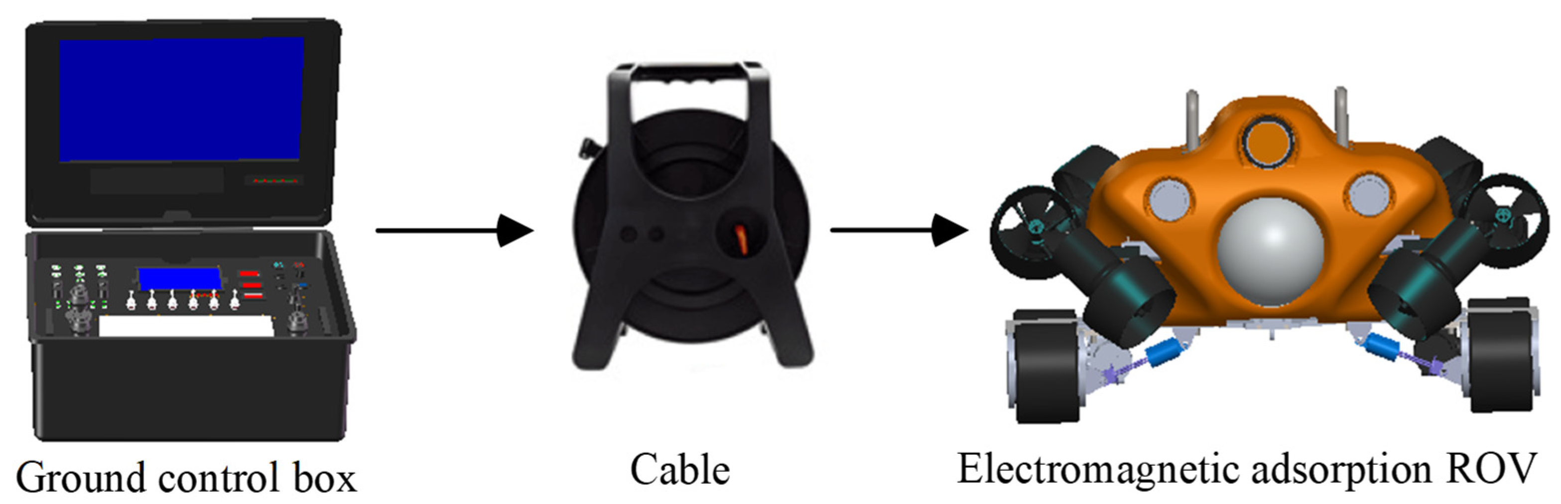
The new ROV system mainly includes the structural system, composed of the ROV and the control box, the control system, composed of the lower computer control program, and the upper computer software. The overall structure of the new ROV system is shown in Figure 1.

The new ROV is mainly composed of the ROV’s buoyancy body in the upper part and the electromagnetic adsorption chassis in the lower part. Because of the special structural design of this ROV, it can complete the conversion of different motion forms. When it is on the ground, the motor on the chassis can be controlled to drive the tire to complete forward, backward, turning, and other actions or the electromagnetic adsorption force on the chassis can be controlled to complete the wall climbing motion on the metal wall. The electromagnetic adsorption chassis of the ROV can be disassembled, and the ROV’s buoyancy body after disassembly can operate independently underwater. The portable ground control box is mainly composed of a control panel, a display screen, an embedded computer, a lithium battery, and other modules. It is connected to the ROV through an umbilical cable to realize power supply and control of the ROV.

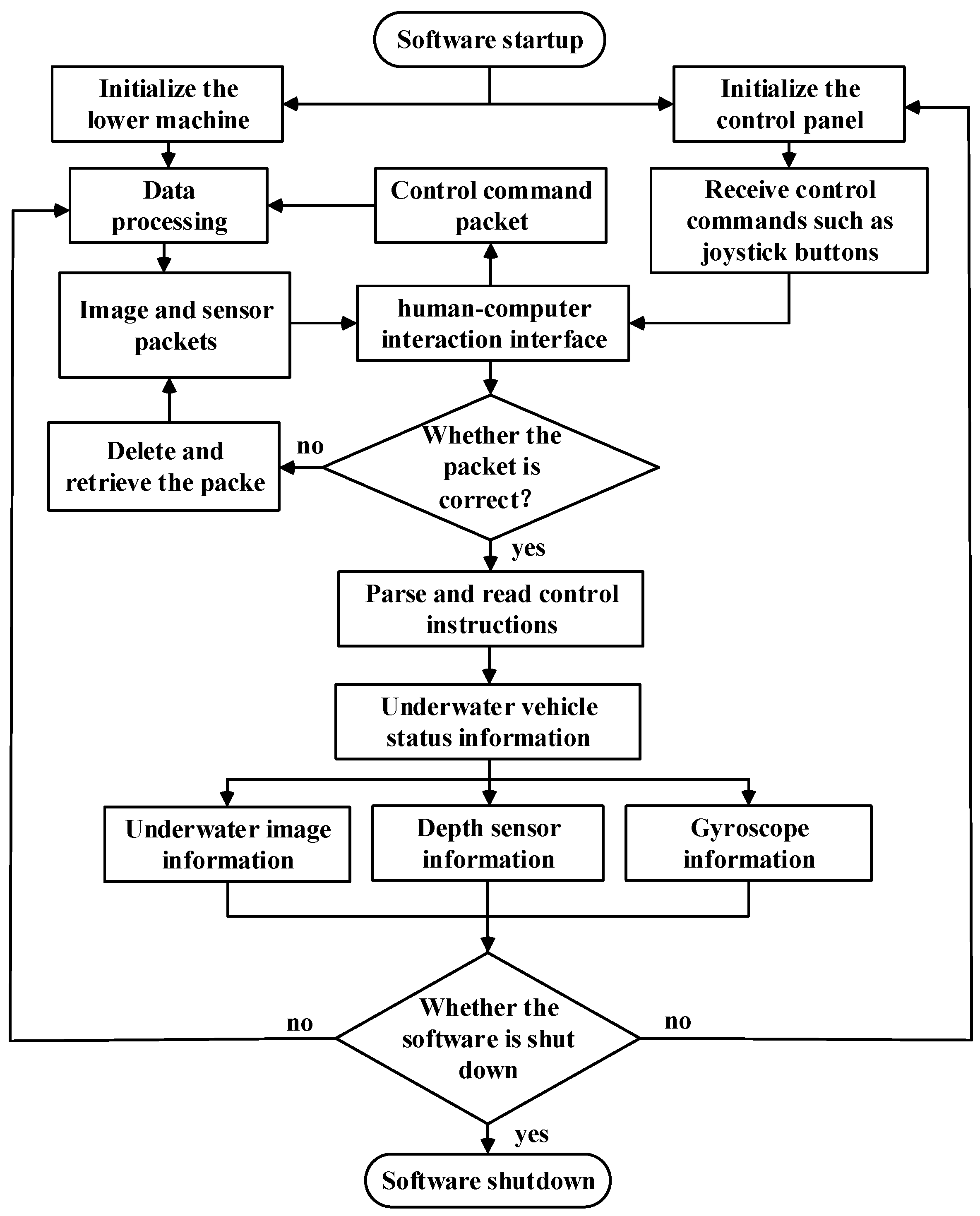
In the control system, the upper computer software visualization window in the portable ground control box can observe the ROV’s video, depth, angle, and other information fed back by the lower computer in real time. The lower computer program is mainly used to analyze and execute various instructions of the upper computer and transmit the instructions to the thrusters, lighting, and other equipment. The upper computer and the lower computer communicate through the power carrier.

3. Structured System Design

3.1. New ROV Structure Design

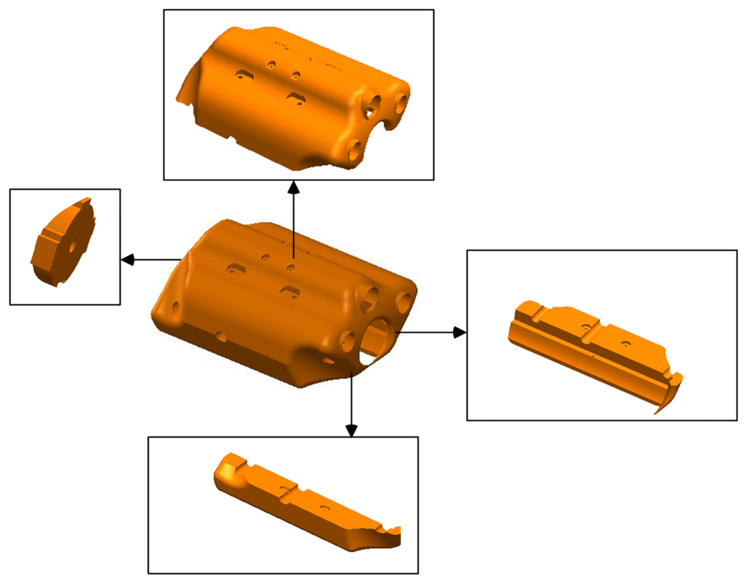
The new ROV is mainly composed of a buoyancy body and an electromagnetic adsorption chassis. The buoyancy body is mainly composed of an electronic cabin, an installation frame, and buoyancy material.

The electronic cabin mainly plays a protective role for its internal electronic equipment. In this paper, the electronic cabin adopts a cylindrical design; the transparent part of the top is acrylic material, and the rest is made of aluminum alloy material. There are two circles of o-shaped grooves at the bottom of the sealing flange and one o-shaped groove at the top. Installation with a sealing ring can achieve better pressure resistance. The interior is equipped with a three-layer circuit board, multiple sensors, and a single degree of freedom pan–tilt camera that can adjust the pitch angle.

The installation framework is the bearing module of the ROV. As shown in Figure 2, the installation frame is made of aluminum alloy, and modules, such as the propeller, the buoyancy material, the electronic cabin, and the electromagnetic adsorption chassis, are fixed onto the aluminum alloy frame. This installation method will make the structure of the ROV more compact and stable. It also gives the whole ROV characteristics of modularization, and the other modules on the ROV can be redesigned according to the relevant requirements. If the size of the original installation hole is retained, the newly designed module can still be installed onto this framework. This design gives the ROV’s structure potential for further optimization.

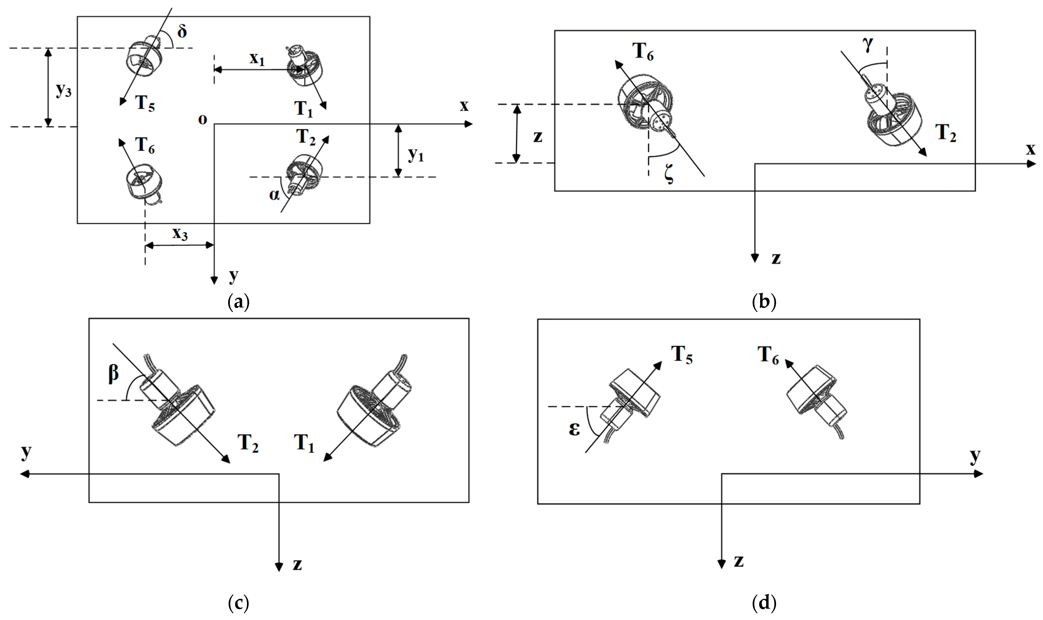
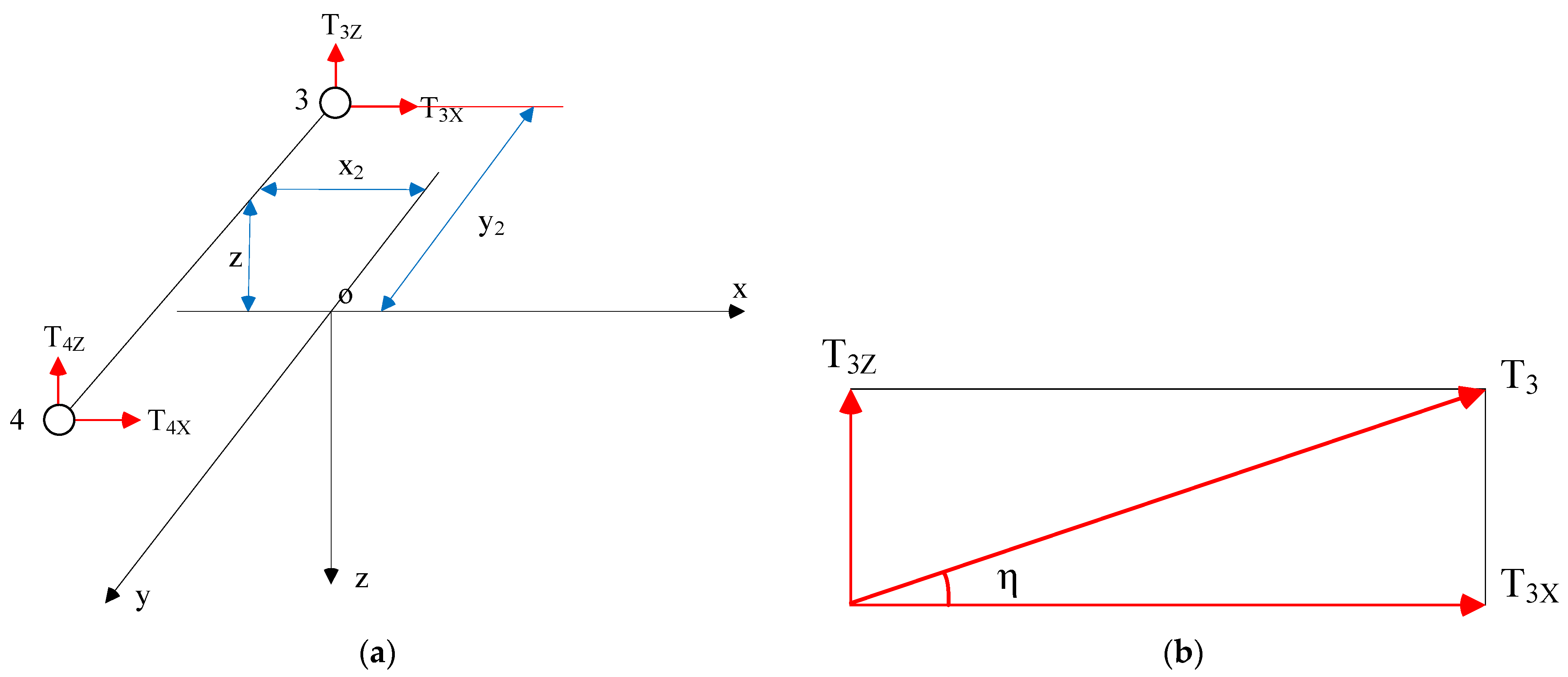
The propeller mainly plays a role in providing power to the ROV. The newly designed ROV is equipped with six propellers. The propeller adopts a more flexible arrangement. The thrust has sufficient force in three degrees of freedom in the longitudinal, transverse, and vertical directions so that the ROV can complete movement in these three directions. The thrust component can produce torque on each axis so that it has enough torque on the other three degrees of freedom to complete rolling, pitching, and yawing motions. The thruster used in the ROV designed in this paper has the advantages of small size, light weight, good sealing, large thrust, low power consumption, and high efficiency. The main performance parameters of the propeller are shown in

Table 1. Underwater thruster performance parameters.

Parameter Name	Parameter Values
Thrust	35 N
Maximum pressure resistance depth	150 m
Rated voltage	24 VDC
Maximum mooring thrust (rated voltage)	3.5 Kgf (forward), 2.6 Kgf (reverse)
Maximum power (rated voltage)	190 W

.

The ROV uses a buoyancy material with a density of 0.25 ${\mathrm{g}/\mathrm{cm}}^3$. While meeting the basic buoyancy requirements of the ROV underwater, the shape of the buoyancy material is designed to be streamlined as much as possible to reduce the resistance of the ROV during operation. As shown in Figure 3, the buoyancy material is composed of four parts, which are fixed on the mounting bracket during installation. The large hole in the middle of the front end of the buoyancy material is used to install the aluminum alloy frame and the electronic cabin. The two symmetrical holes above are used to install the waterproof lighting. The top hole is installed with a monocular camera for underwater visual auxiliary observation.

In the past, most magnetic adsorption chassis adopted the track structure, and the permanent magnet was installed on the track to give the ROV the function of climbing the wall. However, this scheme has obvious disadvantages. First, the track may be loosened during long-term operation, affecting its overall adsorption capacity. Secondly, the permanent magnet is installed on the track, and its magnetic force cannot be changed in the operation of the ROV. If you want to change the size of the adsorption force, you can only change the model of the magnet or change the arrangement density of the magnet on the track, which undoubtedly brings trouble to installation and disassembly. Therefore, this paper designs a structure of a wheeled electromagnetic adsorption chassis, as shown in Figure 4. Five electromagnets with a maximum adsorption force of 150 $\mathrm{N}$ are installed at each end of the chassis. The magnetic force of the electromagnet can be adjusted based on the current size. It can also change the gap between the electromagnet and the contact surface of the chassis by twisting the nut at the upper end of the magnet, thereby changing the magnetic force. The horizontal connection mounting plate is mainly connected by the hinge and the side vertical baffle, and two spring shock absorbers are installed at each end. Under the action of the spring shock absorber, the vertical modules on both sides can bend inward at a certain angle so that they can move on the metal wall with different curvatures. The entire electromagnetic adsorption chassis is equipped with two DC motors to drive the tires [26,27,28].

After assembling each module, the overall structure of the new ROV is shown in Figure 5, and its related design parameters are shown in

Table 2. Design parameters of electromagnetic adsorption ROV.

Parameter Name	Parameter Values
ROV overall dimensions	390 mm × 425 mm × 250 mm
Overall ROV weight	15 kg
Maximum working depth	50 m
Maximum underwater running speed	1 m/s
Maximum wall climbing speed	3 m/min

.

3.2. Portable Ground Control Box Structure’s Design

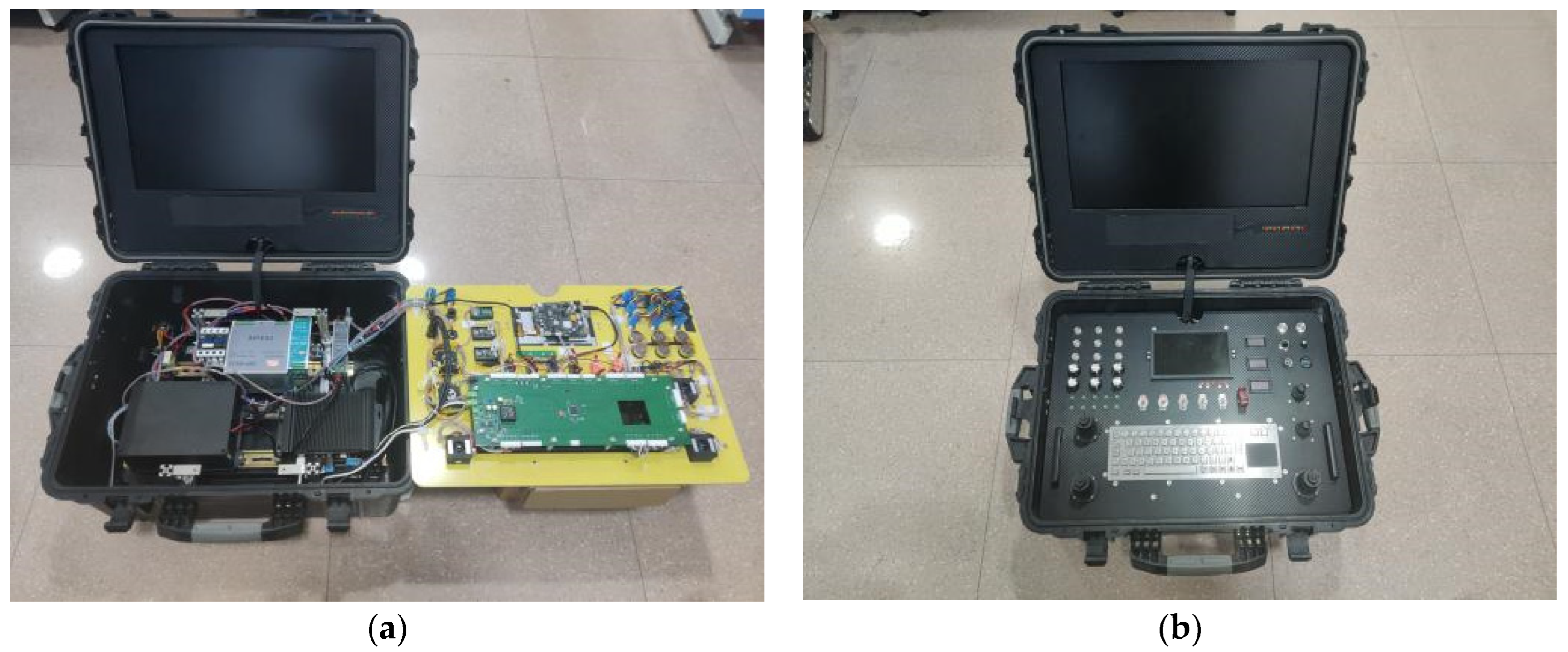
In order to realize control of the new ROV, a portable ground control box integrating control and monitoring is designed. It mainly controls the ROV’s motion through the rocker, knob, and button on the control panel, and it obtains the ROV’s operation information in real time through the visual window of the host computer software. The design of the control box can be divided into three parts, which are the design of the control panel, the design of the hardware installation in the lower box, and the installation design of the upper box’s cover display.

The control panel integrates all rockers, knobs, buttons, etc. that can directly control the ROV. As shown in Figure 6, nine metal waterproof buttons are installed on it for the selection of ROV control modes, such as forward and backward, automatic depth determination, and automatic bow determination mode switching. Six simulation knobs are used to adjust the target depth and angle when the ROV is fixed in depth and heading. Six green LED lights mainly play a role in indicating the rocker switch. Six 2-gear, 2-leg button switches are mainly used to control the opening and closing of the ROV’s lights. Of the two power switches, one is used to control the on–off mode of the overall power supply, and the other is used to control the on–off mode of the ROV’s power supply. In the power supply circuit of the ROV, the maximum fuse current of the fuse is 10 A, which effectively ensures the safety of the ROV’s power supply circuit. The USB 3.0 interface and the network port can be directly connected to the embedded computer without opening the control panel for data transmission and software updates. Three LED digital tube display screens are used for current and voltage display. The embedded metal keyboard is used as the input of the computer in the control box. Three analog rockers are used to control the underwater motion of the ROV. Two digital joysticks are used for control of the ROV’s chassis motor. Two handles are installed on both sides of the control panel, which facilitates the installation and disassembly of the control panel. The parts on the ROV’s control panel are designed with redundancy. When the ROV’s function is expanded, the connection between the control hardware on the panel and the ROV’s expansion function can be established by updating the host computer software to realize control of the ROV’s expansion function.

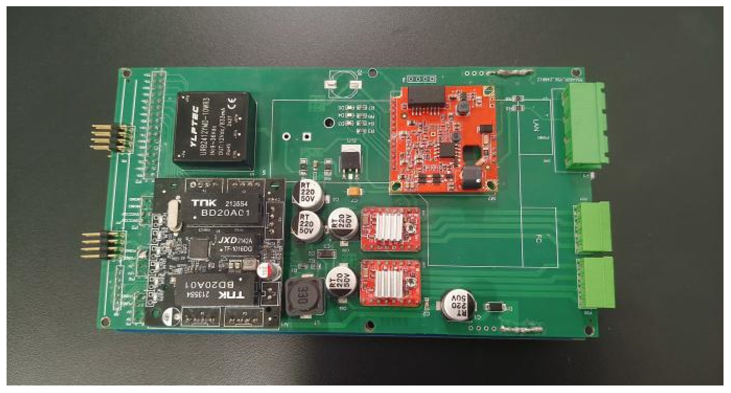
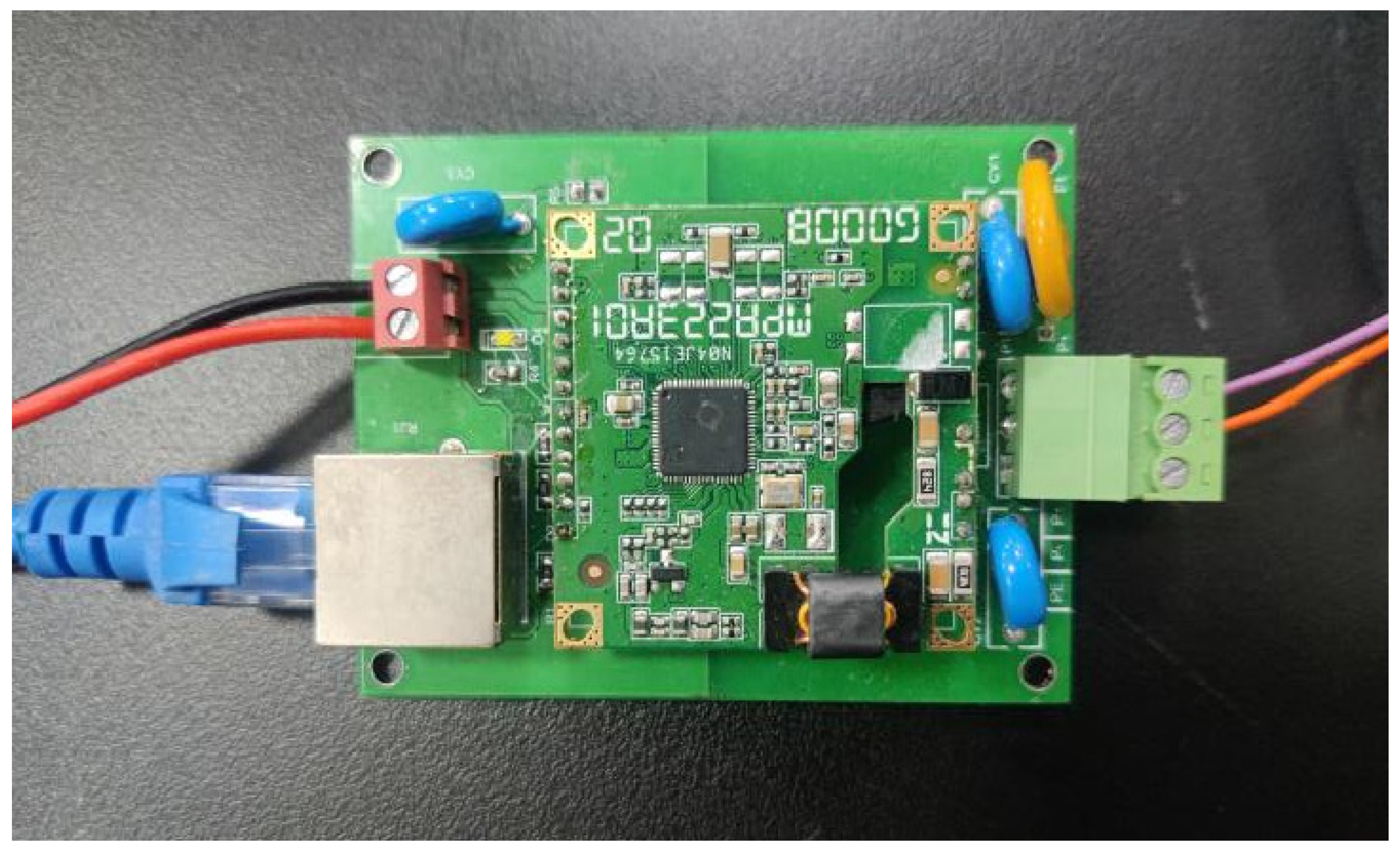
The lower box is mainly used as the installation space for hardware equipment, such as the control panel, the embedded computer, the switching power supply, the power carrier module, the DC contactor, and the lithium battery. Firstly, the fixed frame is designed and installed inside of the box, and the guide rail is installed on the frame so that other equipment can be fixed on the frame through the guide rail buckle. The embedded computer has the basic functions of all computers, but it has a smaller body and a lighter weight than a desktop computer or a laptop, so it is more conducive to assembly in the control box. Two rail-type switching power supplies are used for converting the introduced alternating current into the voltage or current required in the control box. One end of the power carrier module is connected to the embedded computer through the network port, and the other end is connected to the ROV’s electronic cabin through the cable to realize real-time, high-speed communication between the upper computer and the lower computer. The on–off mode of the DC contactor is controlled by the button switch on the control panel, and the output end is connected to the ROV through the cable, which mainly plays the role of protecting the ROV’s power supply line. The control box can supply power to the overall equipment and the ROV by connecting AC power, and a lithium battery can also be installed inside, which can meet the use requirements of the system without an external power supply.

An aluminum alloy mounting plate was designed. The display screen and related electronic drive accessories and adjustment buttons are fixed on the mounting plate through the angular code, and the mounting plate is fixed inside of the upper cover of the control box. The screen and related components are covered and protected by a hard sponge lining.

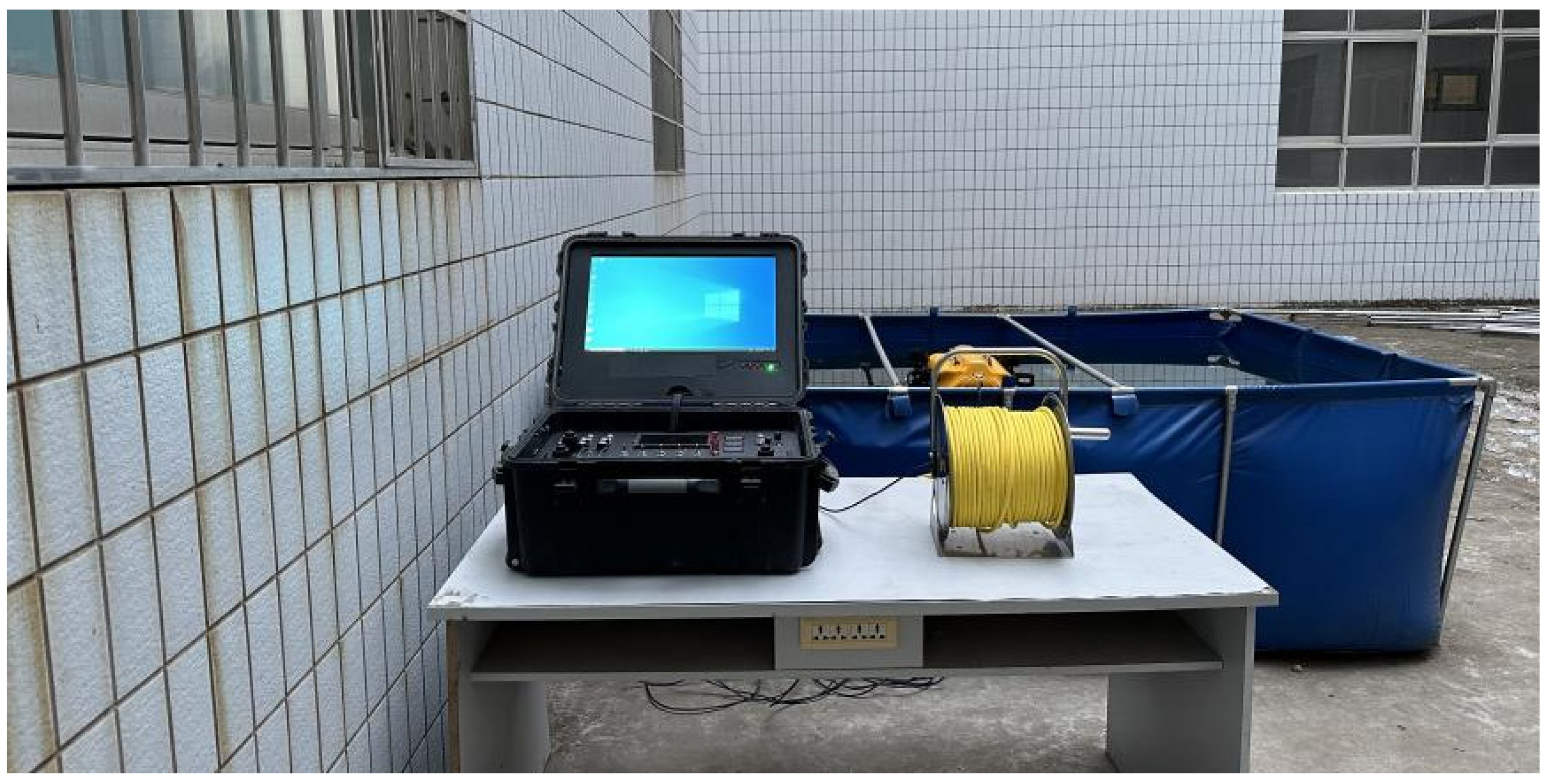
Finally, each module of the control box is assembled and connected. The internal wiring diagram and the physical diagram of the control box are shown in Figure 7.

4. Control System Design

4.1. Control System Hardware Design

The control motherboard is the core hardware of the underwater control system, and its main control chip adopts STM32F103VET6. As shown in Figure 8, the control motherboard consists of three layers of circuit boards. The first layer of the circuit board mainly includes a main control chip, two motor drive modules, a communication module, a power interface, and two underwater lighting interfaces. The second layer of the circuit board mainly includes two waterproof motor interfaces, a depth sensor module, and an attitude sensor module. The third layer of the circuit board is mainly composed of six thruster interfaces and electronic speed modules.

In order to ensure that the digital and analog signals on the control panel can be directly read by the embedded computer, a digital analog acquisition module is designed using an STM32F407VET6 chip. As shown in Figure 9, the acquisition interface for digital and analog signals is designed on the module, which can collect various signals of the rocker, the button, the knob, and other components on the control panel and connect to the embedded computer through USB to a 485 serial port converter. The output end of the 24 V switching power supply is connected to the acquisition module and directly used to supply power to the module. The ROV’s interface on the module outputs a 24 V voltage, which is connected to the DC contactor to supply power to the ROV. The DC voltmeter on the control panel and the battery in the control box are connected to the power interface on the module, and the battery power can be displayed on the voltmeter. The acquisition module is installed on the back of the control panel, which is conducive to the connection between the components on the control panel and the module.

The application of the power carrier module in ROV communication has the advantages of simplifying wiring, improving reliability, real-time data transmission, remote control, and monitoring. Its characteristics of adapting to complex environments, data security, compatibility, and scalability give it broad application prospects in underwater operations. In this paper, power carrier communication is used to communicate between the upper computer and the lower computer, as shown in Figure 10, which is the power carrier module designed in this paper.

4.2. Control System Software Design

The software design of the control system mainly includes the design of the upper computer control software and the writing of the lower computer control program.

The upper computer software of the control box is developed to integrate the various functional modules of the control box. On the one hand, it can allow for human–computer interaction between the operator and the ROV, and the various operations on the control panel can be used to accurately send instructions to the lower computer of the ROV. On the other hand, various feedback information from the ROV can be monitored through the visual interface.

We used C # language to write the code, mainly running on the Windows system. We created a C # WinForm application with an object-oriented design [29].

The host computer software mainly includes the following modules:

(1)

Control box communication module;

(2)

Pid parameter debugging module;

(3)

Control panel command display module;

(4)

Underwater image and sensor display module.

The workflow of the host computer software is shown in Figure 11.

The underwater control program is developed based on STM32 CubeMX and Keil. The Free RTOS real-time operating system is introduced in programming. The process of using the operating system to program the lower computer is as follows [30,31,32]:

(1)

System initialization:

• Initialize hardware peripherals (such as sensors, motors, communication modules, etc.);
• Initialize the FreeRTOS kernel and create tasks, queues, semaphores, and other resources.

(2)

Create tasks:

• Sensor acquisition task: periodically read sensor data (such as depth, attitude, temperature, etc.) and send the data to the queue;
• Motor control task: read control instructions from the queue to control motor motion;
• Communication tasks: communication with the host computer, receiving control instructions and sending sensor data;
• Path planning task: according to the sensor data and task requirements, calculate the motion path and send control instructions;
• Fault detection task: monitor system status, detect faults, and deal with them.

(3)

Start scheduler:

• Start the FreeRTOS scheduler and start task scheduling.

(4)

Task operation:

• Sensor acquisition task: read sensor data and send them to the queue;
• Communication task: receiving instructions from the host computer and sending sensor data;
• Motor control task: read data from the queue and control the motor;
• Path planning task: calculate the path and send control instructions;
• Fault detection task: monitor system status and deal with faults.

(5)

System operation monitoring:

• Monitor the task status, record the log, and ensure the normal operation of the system.

(6)

The end of the system:

• Stop all tasks, close the hardware, and end the system’s operation.

5. Thrust Distribution Layout

5.1. Vector Layout of the Propeller

The distance between the plane where the six thrusters of the ROV are located and the plane $xoy$ where the center of gravity is located is $z$. The four thrusters assembled in the vertical direction are No. 1, No. 2, No. 5, and No. 6, and their thrusts are $T_1$, $T_2$, $T_5$, and $T_6$. The azimuth view of the thruster is shown in Figure 12. The angles between the No. 1 and No. 2 thrusters and the $x$, $y$, and $z$ axes are $\alpha$, $\beta$, and $\gamma$, respectively. The angles between the No. 5 and No. 6 thrusters and the $x$, $y$, and $z$ axes are $\delta$, $\epsilon$, and $\zeta$, respectively. The distance between the No. 1 and No. 2 thrusters and plane $yoz$ is $x_1$, The distance from the plane $xoz$ is $y_1$. The distance between the No. 5 and No. 6 thrusters and plane $yoz$ is $x_3$. The distance from the plane $xoz$ is $y_3$.

The two thrusters assembled in the horizontal direction are No. 3 and No. 4, and their thrusts are $T_3$ and $T_4$, respectively. As shown in Figure 13, the angle between the No. 3 and No. 4 propellers and the $x$-axis is $\eta$, the distance from the plane $yoz$ is $x_2$, and the distance from the plane $xoz$ is $y_2$.

5.2. Thrust Coupling Projection Analysis of the Propulsor

5.2.1. Thrust Projection of the Vertical Thruster

The new ROV is affected by four vertical thrusters at the front and rear. They can provide force and torque in all directions for the ROV. As shown in Figure 14 and Figure 15, the projection analysis of the thrust of the four vertical thrusters is performed. The thrust generated on the $ox$-axis, $oy$-axis, and $oz$-axis is

$$T_{X1}=T_{1X}+T_{2X}-T_{5X}-T_{6X}=T_1\cos \alpha +T_2\cos \alpha -T_5\cos \delta -T_6\cos \delta$$

(1)

$$T_{Y1}=T_{1Y}-T_{2Y}+T_{5Y}-T_{6Y}=T_1\cos \beta -T_2\cos \beta +T_5\cos \epsilon -T_6\cos \epsilon$$

(2)

$$T_{Z1}=T_{1Z}+T_{2Z}-T_{5Z}-T_{6Z}=T_1\cos \gamma +T_2\cos \gamma -T_5\cos \varsigma -T_6\cos \varsigma$$

(3)

The component forces of the No. 1, No. 2, No. 5, and No. 6 propellers on the $x$-axis are $T_{1\mathrm{X}}$, $T_{2\mathrm{X}}$, $T_{5\mathrm{X}}$, and $T_{6\mathrm{X}}$; the component forces on the $y$-axis are $T_{1\mathrm{Y}}$, $T_{2\mathrm{Y}}$, $T_{5\mathrm{Y}}$, and $T_{6\mathrm{Y}}$; and the component forces on the $z$-axis are $T_{1\mathrm{Z}}$, $T_{2\mathrm{Z}}$, $T_{5\mathrm{Z}}$, and $T_{6\mathrm{Z}}$. At this time, the resultant forces of the four thrusters on the three coordinate axes are $T_{X1}$, $T_{Y1}$, and $T_{Z1}$, respectively.

If there is an angle between the four thrusters and any coordinate axis, then the sum of the rolling moment $M_{X1}$, the sum of the pitching moment $M_{Y1}$, and the sum of the yaw moment $M_{Z1}$ generated by the component force on the $ox$-axis, the $oy$-axis, and the $oz$-axis are

$$\begin{array}{l}{M}_{X1}=T_{1Y}z-T_{2Y}z+T_{5Y}z-T_{6Y}z-T_{1Z}{y}_1+T_{2Z}{y}_1+T_{5Z}{y}_3-T_{6Z}{y}_3\\ =T_1\cos \beta z-T_2\cos \beta z+T_5\cos \epsilon z-T_6\cos \epsilon z-T_1\cos \gamma y_1+T_2\cos \gamma y_1+T_5\cos \varsigma y_3+T_6\cos \varsigma y_3\end{array}$$

(4)

$$\begin{array}{l}{M}_{Y1}=-T_{1X}z-T_{2X}z+T_{5X}z+T_{6X}z-T_{1Z}{x}_1-T_{2Z}{x}_1-T_{5z}{x}_3-T_{6Z}{x}_3\\ =-T_1\cos \alpha z-T_2\cos \alpha z+T_5\cos \delta z+T_6\cos \delta z-T_1\cos \gamma x_1-T_2\cos \gamma x_1-T_5\cos \varsigma x_3-T_6\cos \varsigma x_3\end{array}$$

(5)

$$\begin{array}{l}{M}_{Z1}=T_{1X}{y}_1-T_{2X}{y}_1-T_{5X}{y}_3+T_{6X}{y}_3+T_{1Y}{x}_1-T_{2Y}{x}_1-T_{5Y}{x}_3+T_{6Y}{x}_3\\ =T_1\cos \alpha y_1-T_2\cos \alpha y_1-T_5\cos \delta y_3+T_6\cos \delta y_3+T_1\cos \beta x_1-T_2\cos \beta x_1-T_5\cos \epsilon x_3+T_6\cos \epsilon x_3\end{array}$$

(6)

5.2.2. Thrust Projection of the Horizontal Thruster

The new ROV is affected by two horizontal thrusters, which can provide horizontal force and a small amount of vertical force for the ROV. The projection analysis of the thrust of the two horizontal thrusters is shown in Figure 16. The thrust generated in the $ox$-axis, the $oy$-axis, and the $oz$-axis is

$$T_{X2}=T_{3X}+T_{4X}=T_3\cos \eta +T_4\cos \eta$$

(7)

$$T_{Y2}=0$$

(8)

$$T_{Z2}=-T_{3Z}-T_{4Z}=-T_3\sin \eta -T_4\sin \eta$$

(9)

The component forces of the No. 3 and No. 4 propellers on the $x$-axis are $T_{3\mathrm{X}}$ and $T_{4\mathrm{X}}$; the component forces on the $y$-axis are $T_{3\mathrm{Y}}$ and $T_{4\mathrm{Y}}$; and the component forces on the $z$-axis are $T_{3\mathrm{Z}}$ and $T_{4\mathrm{Z}}$. The resultant forces of the two propellers on $x$, $y$, and $z$ are $T_{X2}$, $T_{Y2}$, and $T_{Z2}$, respectively.

The sum of the rolling moment of the two horizontal thrusters in the $ox$-axis, the $oy$-axis, and the $oz$-axis is $M_{X2}$, the sum of the pitching moment is $M_{\mathrm{Y}2}$, and the sum of the yaw moment is $M_{\mathrm{Z}2}$:

$$M_{X2}=T_{3Z}{y}_2-T_{4Z}{y}_2=T_3\sin \eta y_2-T_4\sin \eta y_2$$

(10)

$$M_{Y2}=-T_{3X}z-T_{4X}z-T_{3Z}{x}_2-T_{4Z}{x}_2=-T_3\cos \eta z-T_4\cos \eta z-T_3\sin \eta x_2-T_4\sin \eta x_2$$

(11)

$$M_{Z2}=T_{3X}{y}_2-T_{4X}{y}_2=T_3\cos \eta y_2-T_4\cos \eta y_2$$

(12)

5.2.3. Total Thrust of the Propulsion System

After the above derivation, the total thrust $T_X$, $T_Y$, and $T_Z$ of the six thrusters in the new ROV propulsion system on the three coordinate axes is

$$T_X=T_{X1}+T_{X2}=T_1\cos \alpha +T_2\cos \alpha +T_3\cos \eta +T_4\cos \eta -T_5\cos \delta -T_6\cos \delta$$

(13)

$$T_Y=T_{Y1}+T_{Y2}=T_1\cos \beta -T_2\cos \beta +T_5\cos \epsilon -T_6\cos \epsilon$$

(14)

$$T_Z=T_{Z1}+T_{Z2}=T_1\cos \gamma +T_2\cos \gamma -T_3\sin \eta -T_4\sin \eta -T_5\cos \varsigma -T_6\cos \varsigma$$

(15)

The total thrust torque $M_X$, $M_Y$, and $M_Z$ of the six thrusters in the three coordinate axes is

$$\begin{array}{l}{M}_X=M_{X1}+M_{X2}=T_1\cos \beta z-T_1\cos \gamma y_1-T_2\cos \beta z+T_2\cos \gamma y_1+T_3\sin \eta y_2\\ -T_4\sin \eta y_2+T_5\cos \epsilon z+T_5\cos \varsigma y_3-T_6\cos \epsilon z-T_6\cos \varsigma y_3\end{array}$$

(16)

$$\begin{array}{l}{M}_Y=M_{Y1}+M_{Y2}=-T_1\cos \alpha z-T_1\cos \gamma x_1-T_2\cos \alpha z-T_2\cos \gamma x_1-T_3\cos \eta z\\ -T_3\sin \eta x_2-T_4\cos \eta z-T_4\sin \eta x_2+T_5\cos \delta z-T_5\cos \varsigma x_3+T_6\cos \delta z-T_6\cos \varsigma x_3\end{array}$$

(17)

$$\begin{array}{l}{M}_Z=M_{Z1}+M_{Z2}=T_1\cos \alpha y_1+T_1\cos \beta x_1-T_2\cos \alpha y_1-T_2\cos \beta x_1\\ +T_3\cos \eta y_2-T_4\cos \eta y_2-T_5\cos \delta y_3-T_5\cos \epsilon x_3+T_6\cos \delta y_3+T_6\cos \epsilon x_3\end{array}$$

(18)

The above three equations can be generalized. The six degrees of freedom thrust and thrust torque generated by the six thrusters on the ROV are

$$T=\left[\begin{array}{c}{T}_X\\ T_Y\\ T_Z\\ M_X\\ M_Y\\ M_Z\end{array}\right]=B(\theta )\left[\begin{array}{c}{T}_1\\ T_2\\ T_3\\ T_4\\ T_5\\ T_6\end{array}\right]=B(\theta )U$$

(19)

In the formula,

• $U$—thrust vector matrix of the thruster output, $U={\left[\begin{array}{cccccc}{T}_1& T_2& T_3& T_4& T_5& T_6\end{array}\right]}^T$;
• $B(\theta )$—vector placement matrix of the thruster.

The vector arrangement matrix of the ROV propulsion system is

$$\begin{array}{l}B(\theta )=\left[\begin{array}{ccc}\cos \alpha & \cos \alpha & \cos \eta \\ \cos \beta & -\cos \beta & 0\\ \cos \gamma & \cos \gamma & -\sin \eta \\ \cos \beta z-\cos \gamma y_1& -\cos \beta z+\cos \gamma y_1& \sin \eta y_2\\ -\cos \alpha z-\cos \gamma x_1& -\cos \alpha z-\cos \gamma x_1& -\cos \eta z-\sin \eta x_2\\ \cos \alpha y_1+\cos \beta x_1& -\cos \alpha y_1-\cos \beta x_1& \cos \eta y_2\end{array}\right.\\ \left.\begin{array}{ccc}\cos \eta & -\cos \delta & -\cos \delta \\ 0& \cos \epsilon & -\cos \epsilon \\ -\sin \eta & -\cos \varsigma & -\cos \varsigma \\ -\sin \eta y_2& \cos \epsilon z+\cos \varsigma y_3& -\cos \epsilon z-\cos \varsigma y_3\\ -\cos \eta h-\sin \eta x_2& \cos \delta z-\cos \varsigma x_3& \cos \delta z-\cos \varsigma x_3\\ -\cos \eta y_2& -\cos \delta y_3-\cos \epsilon x_3& \cos \delta y_3+\cos \epsilon x_3\end{array}\right]\end{array}$$

(20)

6. Simulation Analysis of Thrust Allocation

6.1. Direct Logic Method

Assuming that the ROV is affected by the longitudinal thrust, the lateral thrust, and the pitching moment, it presents a compound motion state. According to the characteristics of the vector arrangement of the ROV thrusters, the longitudinal thrust, the lateral thrust, and the pitching moment can be distributed according to the following formula, such that the expected thrust $T_{E1}$, $T_{E2}$, $T_{E3}$, $T_{E4}$, $T_{E5}$, and $T_{E6}$ of each thruster is as follows:

The expected distribution thrust of the No. 1 thruster:

$$T_{E1}=T_X+T_Y-M_Y$$

(21)

The expected distribution thrust of the No. 2 thruster:

$$T_{E2}=T_X-T_Y-M_Y$$

(22)

The expected distribution thrust of the No. 3 thruster:

$$T_{E3}=T_X-M_Y$$

(23)

The expected distribution thrust of the No. 4 thruster:

$$T_{E4}=T_X-M_Y$$

(24)

The expected distribution thrust of the No. 5 thruster:

$$T_{E5}=-T_X+T_Y+M_Y$$

(25)

The expected distribution thrust of the No. 6 thruster:

$$T_{E6}=-T_X-T_Y+M_Y$$

(26)

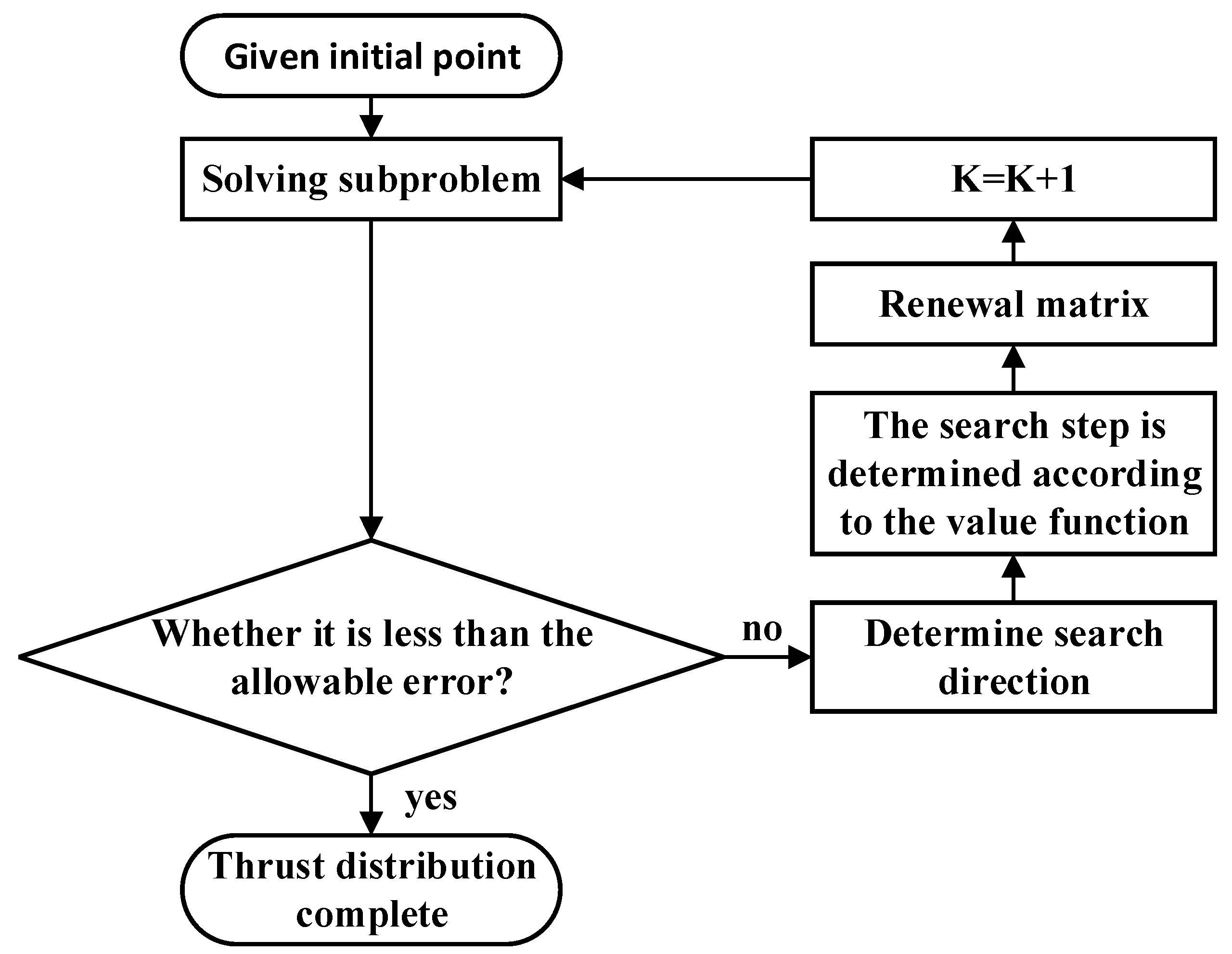
6.2. Sequential Quadratic Programming Method

The essence of using SQP to solve the optimal solution is to solve a series of quadratic programming subproblems. For nonlinear constrained optimization problems [33,34,35],

$$\begin{array}{l}\min f(x)\\ s.t.\left\{\begin{array}{c}{h}_i(x)=0,i\in E=\left\{1,2,\cdots ,m_1\right\}\\ g_j(x)\ge 0,j\in I=\{m_1+1,m_1+2,\cdots ,m_1+m_2\}\end{array}\right.\end{array}$$

(27)

In the formula, $x$ is a variable, $f(x)$ is an objective function, $h_i(x)$ is a nonlinear equality constraint, and $g_i(x)$ is a nonlinear inequality constraint.

Let $E=\{1,2,\cdots ,m_1\}$ be the sequence set of equality constraints and let $I=\{m_1+1,m_1+2,\cdots ,m_1+m_2\}$ be the sequence set of inequality constraints.

The equation constraint can be written as

$$c_E(x)={[c_1(x)c_2(x)\cdots c_{m_1}(x)]}^T=0$$

(28)

The inequality constraint is notated as

$$c_I(x)={[c_{m_1+1}(x)c_{m_1+2}(x)\cdots c_{m_1+m_2}(x)]}^T=0$$

(29)

Nonlinear constrained optimization can be written as

$$\begin{array}{l}\min f(x)\\ s.t.\left\{\begin{array}{c}{c}_E(x)=0\\ c_I(x)\ge 0\end{array}\right.\end{array}$$

(30)

Then, the Lagrangian function of the above equation is

$$L\left(x,\lambda ,\mu \right)=f(x)-{\lambda }^T{c}_E(x)-{\mu }^T{c}_I(x)$$

(31)

where $\lambda$ and $\mu$ are Lagrangian ordinary numbers.

$c_E(x)$ and $c_I(x)$ are the Jacobi matrices:

$$J_E=\nabla c_E(x)={[\nabla c_1(x)\nabla c_2(x)\cdots \nabla c_{m_1}(x)]}^T$$

(32)

$$J_I=\nabla c_I(x)={[\nabla c_{m_1+1}(x)\nabla c_{m_1+2}(x)\cdots \nabla c_{m_1+m_2}(x)]}^T$$

(33)

Then, the gradient vector of the Lagrangian function is

$$\nabla L(x,\lambda ,\mu )=\left[\begin{array}{c}{\nabla }_{x}L(x,\lambda ,\mu )\\ {\nabla }_{\lambda }L(x,\lambda ,\mu )\\ {\nabla }_{\mu }L(x,\lambda ,\mu )\end{array}\right]=\left[\begin{array}{c}g(x)-J_E{(x)}^T\lambda -J_I{(x)}^T\mu \\ -c_E(x)\\ -c_I(x)\end{array}\right]$$

(34)

where $g(x)\in R^3$ is the gradient of $f(x)$.

$\nabla L(x,\lambda ,\mu )$ The Jacobi matrices with respect to $x$, $\lambda$, and $\mu$ are

$$\begin{array}{ll}{\nabla }^{2}L(x,\lambda ,\mu )& =\left[\begin{array}{ccc}{{\nabla }^2}_{xx}L(x,\lambda ,\mu )& {{\nabla }^2}_{x\lambda }L(x,\lambda ,\mu )& {{\nabla }^2}_{x\mu }L(x,\lambda ,\mu )\\ {{\nabla }^2}_{\lambda x}L(x,\lambda ,\mu )& {{\nabla }^2}_{\lambda \lambda }L(x,\lambda ,\mu )& {{\nabla }^2}_{\lambda \mu }L(x,\lambda ,\mu )\\ {{\nabla }^2}_{\mu x}L(x,\lambda ,\mu )& {{\nabla }^2}_{\mu \lambda }L(x,\lambda ,\mu )& {{\nabla }^2}_{\mu \mu }L(x,\lambda ,\mu )\end{array}\right]\\ & =\left[\begin{array}{ccc}W(x,\lambda ,\mu )& -J_E{(x)}^T& -J_I{(x)}^T\\ -J_E(x)& 0& 0\\ -J_I(x)& 0& 0\end{array}\right]\end{array}$$

(35)

In the formula,

$$W(x,\lambda ,\mu )=H(x)-{\displaystyle \sum _{i=1}^{m_1}{\lambda }_i{\nabla }^2{c}_i(x)-}{\displaystyle \sum _{i=m_1+1}^{m_1+m_2}{\mu }_{i-m_1}{\nabla }^2{c}_i(x)}$$

(36)

$H(x)\in R^3$ is the Hessian matrix of $f(x)$.

Then, the Karush–Kuhn–Tucker (derivative with respect to the Lagrangian) condition for the above equation is

$$\left\{\begin{array}{c}{\nabla }_{x}L(x^{\ast },{\lambda }^{\ast },{\mu }^{\ast })=g(x^{\ast })-J_E{(x^{\ast })}^T{\lambda }^{*}-J_I{(x^{\ast })}^T{\mu }^{\ast }=0\\ {\nabla }_{\lambda }L(x^{*},{\lambda }^{*},{\mu }^{*})=-c_E(x^{*})=0\\ {\nabla }_{\mu }L(x^{*},{\lambda }^{*},{\mu }^{*})=-c_I(x^{*})\le 0\\ M^{*}{c}_I(x^{*})=0\\ {\mu }^{*}\ge 0\end{array}\right.$$

(37)

The Taylor expansion of the above equation is equivalent to finding an optimal solution to a quadratic programming problem:

$$\begin{array}{l}\min {\displaystyle \frac{1}{2}}{({\delta }_x)}^{T}W(x^k,{\lambda }^k,{\mu }^k){\delta }_x+{({\delta }_x)}^T{\nabla }_{x}L(x^k,{\lambda }^k,{\mu }^k)\\ s.t.\left\{\begin{array}{c}{J}_E(x^k){{\delta }_x}^k=-c_E(x^k)\\ J_I(x^k){{\delta }_x}^k=-c_I(x^k)\end{array}\right.\end{array}$$

(38)

The basic process of the sequential quadratic programming method is shown in Figure 17.

6.3. Objective Function and Constraint Conditions of Thrust Allocation

The objective function of thrust allocation can be set to [36,37,38]

$$J(\alpha ,u,s)=u^{T}Wu+s^{T}Qs+{\displaystyle \frac{\rho }{\epsilon +\det (B(\alpha )B{(\alpha )}^T)}}$$

(39)

In the formula, $\alpha$ is the azimuth angle of each propeller; $u$ is the thrust generated by each propeller; and, as a relaxation variable, $s$ is a column matrix, which represents the difference between the thrust input by the controller and the thrust after the thrust synthesis output so as to ensure that the thrust allocation problem always has a feasible solution.

The definition of the right end of the above equation is as follows:

• The first term is used to optimize energy consumption. $W$ is the energy consumption weight matrix, which is a diagonal matrix. The weight of energy consumption in each optimization objective can be changed by changing its size. Optimizing this item can also reduce the wear degree of the propeller and make the propeller work more safely and stably.
• The second term belongs to the penalty term. $Q$ is also a diagonal matrix, which can determine the weight of the error value of input and output in the objective function by changing the value of $Q$.
• The third item is set to avoid the singular structure of the thruster, where $\epsilon$ is the number greater than 0 and a is the weight of the optimization item in order to avoid the denominator being 0.

According to the analysis of the actual situation of the ROV, the constraints of thrust distribution are divided into equality constraints and inequality constraints.

The equality constraint is

$$s=\tau -B(\alpha )u$$

(40)

In the formula, $\tau$ is the input thrust of the controller and $B(\alpha )$ is the vector layout matrix of the propulsion system.

The constraint condition represents the relationship between the error between the input of the controller and the output of the thrust synthesis and the relaxation variable, allowing the existence of the error, in order to better complete the task of thrust distribution.

The inequality constraint is

$$\begin{array}{c}{u}_{\min }\le u\le u_{\max }\\ \Delta u_{\min }\le \Delta u\le \Delta u_{\max }\end{array}$$

(41)

In the formula, $u_{\min }$ is the minimum thrust of the propeller, $u_{\max }$ is the maximum thrust of the propeller, and $u_0$ is the thrust at the previous moment.

This constraint limits the output range of the propeller, which can prevent the loss of the propeller and the low efficiency of the underwater operation caused by exceeding the maximum thrust.

6.4. Establishment of the Simulation Model

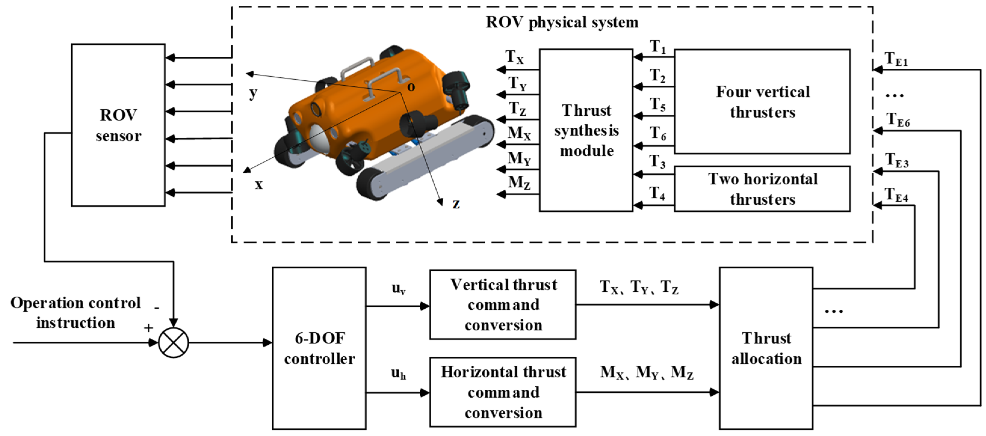
According to the principle of ROV motion control and the needs of practical work, the composition and the working principle of the motion control system are shown in Figure 18 [39,40].

According to the composition and working principle of the above control system, in the process of simulation, the basic model of simulation is shown in Figure 19.

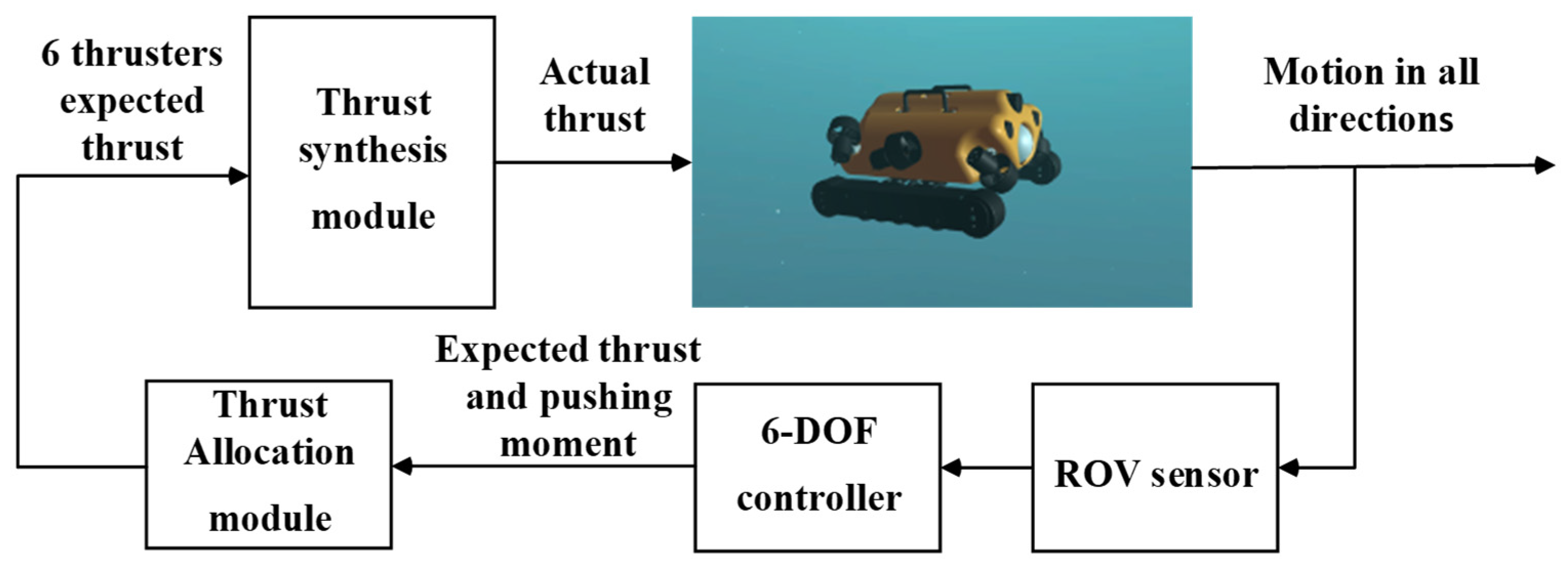
The simulation model of the ROV control system is mainly composed of several modules in the above figure. The 6 degrees of freedom controller reads the control input of the rocker to obtain the expected thrust and torque of a certain degree of freedom. The thrust distribution module calculates the thrust and the thrust required for each thruster. The thrust synthesis module synthesizes the components of the six thrusters to determine the actual thrust and the thrust torque required for the ROV’s motion, and then it drives the ROV’s motion. Because the control system is a closed-loop system, the actual motion of the ROV can be returned to the 6 degrees of freedom controller through the sensor module, and real-time adjustment of the ROV’s motion can be completed.

6.5. Thrust Distribution Simulation Analysis

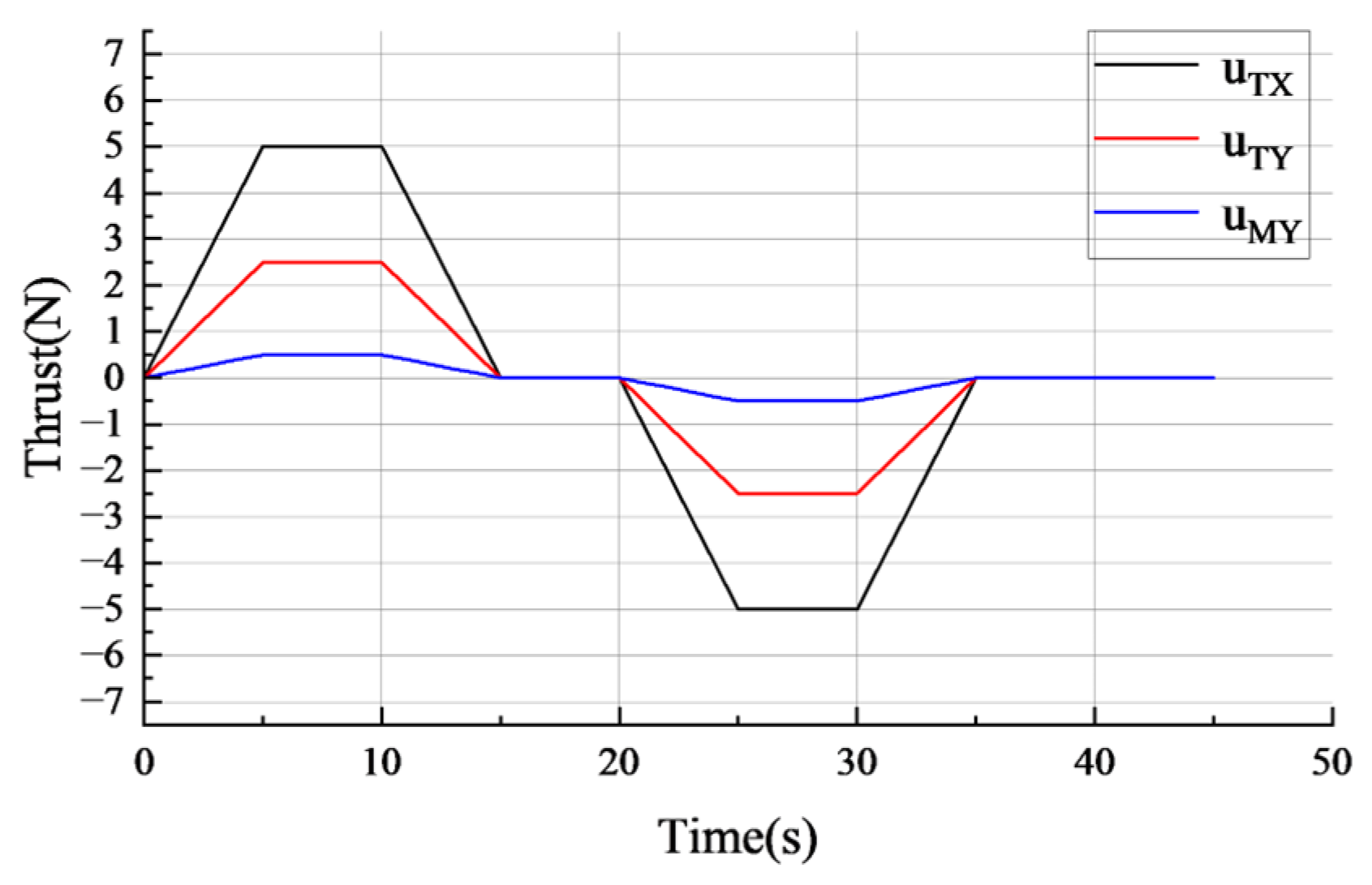
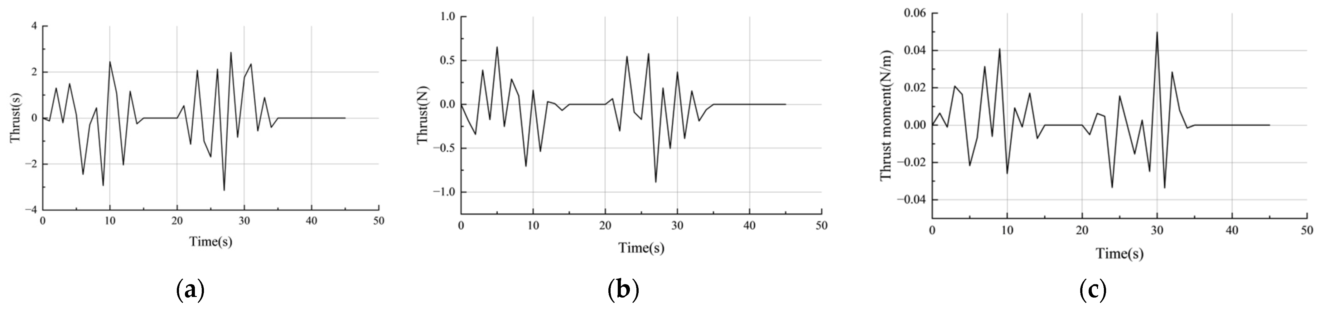
The simulation model of the new ROV’s motion control and thrust allocation is established in MATLAB, and thrust allocation is carried out using a direct logic method and a sequential quadratic programming method. The rocker is used to randomly input the voltage of three degrees of freedom of longitudinal, transverse, and pitch output. Firstly, the rocker is slowly moved to slowly increase the output voltage. When the output value reaches a certain output value, the rocker is stopped and kept in this state for a period of time. After that, the rocker is slowly released to slowly reduce the output. After reaching the zero input state for a period of time, the rocker is moved backward to obtain the curve of the output voltage of the rocker with time.

It is known that the maximum thrust of each propeller is 35 $\mathrm{N}$ at forward rotation and 26 $\mathrm{N}$ at reverse rotation. As shown in Figure 20, $u_{TX}$, $u_{TY}$, and $u_{MY}$ represent the voltage corresponding to the longitudinal, transverse, and rolling output of the rocker, respectively. Where $u_{TX}\in [-5,5]$ and when $u_{TX}=5\mathrm{V}$, the corresponding maximum longitudinal thrust is 128 $\mathrm{N}$; where $u_{TY}\in [-5,5]$ and when $u_{TY}=5\mathrm{V}$, the corresponding maximum lateral thrust is 62 $\mathrm{N}$; among them, for $u_{MY}\in [-5,5]$, when $u_{MY}=5\mathrm{V}$, the corresponding maximum rolling moment is 17 $\mathrm{N}/\mathrm{m}$.

It can be seen from Figure 21 that after thrust distribution using the direct logic method and the sequential quadratic programming method, under the direct logic method, the six thrusters, whether forward or reverse, exceed the maximum thrust that may occur in their thrusters to varying degrees, that is, the phenomenon of thrust saturation. This shows that although the direct logic method is simple, it does not consider the maximum thrust limit of the thruster. When running in this state, there will be problems, such as thruster overload, hardware damage, control performance degradation, and increased ROV power consumption. However, under the sequential quadratic programming method, the six thrusters do not exceed their maximum values during forward and reverse rotation, indicating that the sequential quadratic programming method can optimize the thrust distribution of the thruster and avoid oversaturation of the thrust output.

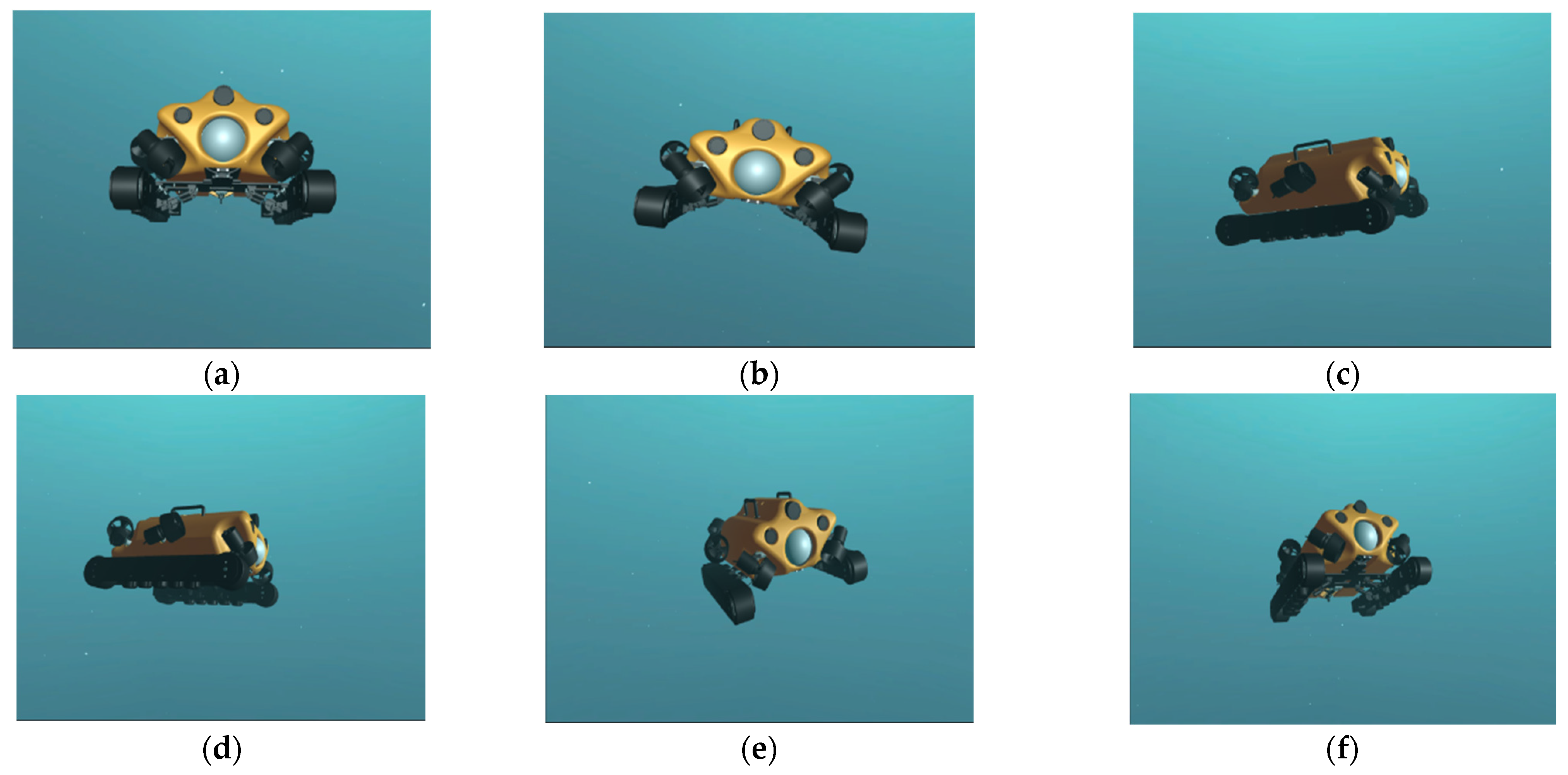
The Unity 3D simulation experiment platform is developed using C# language. The related code for the thrust distribution control algorithm based on sequential quadratic programming is written into a script file in C# language, which is imported into the simulation system and mounted onto the ROV model. This platform simulates the approximate real environment of an ROV working underwater, and the results are more general than those of a MATLAB simulation. By connecting the rocker, different forces or torques are input to the different degrees of freedom of the ROV, and the running attitude of the ROV is observed through the visual window.

As shown in Figure 22, the thrust of one degree of freedom, the thrust and torque of two degrees of freedom, and the thrust and torque of three degrees of freedom are input into the Unity 3D platform. The attitude of the ROV in the simulated state can meet the expected control requirements. This simulation further verifies the feasibility of the sequential quadratic programming method to optimize the thrust distribution of the developed ROV.

7. Experiment

7.1. Attitude Control Experiment

The basic functions of the designed and assembled ROV and the control box are tested. After meeting the experimental requirements, the ROV is connected to the control box using a cable to carry out the underwater attitude control experiment of the ROV.

In the experiment, the attitude control of the ROV is carried out by shaking the rocker. The overall operating state of the ROV under different thrust input conditions is compared. The construction of the whole pool experimental platform is shown in Figure 23.

Firstly, the simulation results are verified, and the same instructions as the simulation are input. The thrust and torque changes of each propeller are observed and recorded and then compared with the output force and torque. The error between the actual value and the theoretical value is calculated and drawn, and the curve of Figure 24 is drawn.

By observing and analyzing the above change curve, it can be clearly seen that after the thrust distribution of the sequential quadratic programming method, the error between the actual value and the theoretical value is about 3%, and the error is within a reasonable range. This shows that the thrust distribution of the developed ROV using sequential quadratic programming can meet the expected demand and produce a better thrust distribution result.

Next, the new ROV motion control experiment is carried out, and different degrees of freedom control are input. The motion state of the ROV is shown in Figure 25.

As shown in Figure 25, the body of the ROV will not oscillate during operation, and the attitude is relatively stable, indicating that the thrust distribution error of each thruster of the ROV is within a reasonable range and the feasibility of the thrust distribution control algorithm at this time. The sequential quadratic programming method can be applied to the optimization of the thrust distribution problem of the new ROV.

7.2. Application Scenario Simulation Experiment

The new ROV system designed in this paper is mainly used in the detection of marine engineering facilities, so the working ability of the ROV in the actual working environment was tested. The steel pipe was used as the target detection object of the ROV, and a white mark was made on the steel pipe to simulate the defects on the steel pipe. The ROV was operated using the ground control box to carry out all-round detection of the steel pipe. After the defects on the steel pipe were found through the visual interface of the upper computer, the ROV was controlled and hovered in the appropriate position, and the defects could be clearly seen. At this time, the ROV can be manipulated to take photos and record the ROV’s depth information displayed by the upper computer software interface. As shown in Figure 26, the actual image of the ROV for underwater target detection shows that the ROV can basically complete the detection task for engineering facilities underwater.

8. Conclusions

In this paper, a new ROV system and its thrust allocation optimization method are proposed for the detection requirements of marine engineering facilities. The main points of the research can be summarized as follows:

• System design: The ROV’s body with an electromagnetic adsorption chassis, a buoyancy mechanism, and an installation framework is constructed, and the portable ground control box and the control system, including the upper computer software and the lower computer program, are developed to realize the efficient coordination of the upper computer and the lower computer.
• Thrust allocation optimization: Based on the vector layout of the ROV’s thruster, the thrust–torque mathematical model is established, and the optimization problem is designed to solve the ROV’s thrust allocation as the goal and the thruster’s saturation as the constraint. Through MATLAB and Unity 3D simulation, the simulation results of the direct logic method and sequential quadratic programming (SQP) are compared, which shows the advantages of the SQP algorithm in solving the thrust allocation problem.
• Experimental verification: The underwater experimental platform is built to complete the motion control experiment. The experiment verifies the accuracy of the simulation results and proves the engineering application feasibility of the SQP optimization method. The simulation scene observation experiment shows that the system can stably complete the underwater inspection task and meet the expected design requirements.
• Future research will focus on the following three aspects: first, lightweight improvement of the electromagnetic adsorption chassis to reduce the complexity of thrust distribution; second, optimizing the layout of the propulsion system and developing a more robust adaptive allocation algorithm; and thirdly, carrying out a field test in the marine environment to verify the reliability of the system under complex working conditions, especially the dynamic response performance under strong current disturbance and multi-obstacle scenarios.

References

1. Nauert, F.; Kampmann, P. Inspection and maintenance of industrial infrastructure with autonomous underwater robots. Front. Robot. AI 2023, 10, 1240276. [Google Scholar] [CrossRef] [PubMed]
2. Ren, F.S.; Wang, Z.Y. Design and Implementation of Small Modular Amphibious Robot System. Processes 2024, 12, 2355. [Google Scholar] [CrossRef]
3. Li, P.; Wei, Z.K.; Li, H.B. Application and Prospect of AUV Navigation System. Navig. Control 2023, 22, 8–20. [Google Scholar]
4. Wang, J.Y.; Ke, W. Development plan of unmanned system and development status of uuv technology in foreign countries. J. Robot. Control 2022, 3, 187–195. [Google Scholar] [CrossRef]
5. Sahoo, A.; Santosha, K.D.; Robi, P.S. Design of a compact rov for river exploration. In Proceedings of the 2017 3rd International Conference on Advances in Robotics, New Delhi, India, 28 June–2 July 2017. [Google Scholar]
6. Li, J.; Xu, J.C.; Zhan, K. Analysis of Hydrodynamic Characteristics of ROV for Underwater Inspection of Deep Sea Mining. J. Ocean. Technol. 2024, 43, 25–33. [Google Scholar]
7. Xu, D.Y.; Ling, H.J. A closed streamlined observation stage ROV design. Ship Sci. Technol. 2018, 40, 143–148. [Google Scholar]
8. Aguirre, C.; Oscar, A. Design and Construction of an ROV for Underwater Exploration. Sensors 2019, 19, 5387. [Google Scholar] [CrossRef]
9. Kabanov, A.; Kramar, V.; Ermakov, I. Design and modeling of an experimental rov with six degrees of freedom. Drones 2021, 5, 113. [Google Scholar] [CrossRef]
10. Du, X.Y.; Yang, P.; Zhang, M.L. Design and Experiment of Modular Wall-climbing Robot. Mech. Sci. Technol. Aerosp. Eng. 2024, 43, 1180–1188. [Google Scholar]
11. Zhang, X.; Zhang, M.; Jiao, S.; Sun, L.; Li, M. Design and Optimization of the Wall Climbing Robot for Magnetic Particle Detection of Ship Welds. J. Mar. Sci. Eng. 2024, 12, 610. [Google Scholar] [CrossRef]
12. Gao, Y.; Lu, L.P. Structural design and optimization of permanent magnet adsorption unit of water-wall detection climbing robot. J. Tianjin Univ. Technol. 2024, 1–12. Available online: https://link.cnki.net/urlid/12.1374.n.20241029.1908.022 (accessed on 19 February 2025).
13. Qiu, S.C.; Wu, J.B. Body Design of a Storage Tank Wall-climbing Robot Based on Magnetic Adsorption. China Mech. Eng. 2022, 33, 270–278. [Google Scholar]
14. Chen, Y.; Ke, X.Y.; Zhou, R.R.; Wan, X.J.; Guo, J.T.; Li, X.H. Numerical Simulation of Hydraulic Characteristics in Annular Jet Propulsion System for Underwater Spherical Robot. J. Nanjing Inst. Technol. (Nat. Sci. Ed.) 2024, 22, 1–10. [Google Scholar]
15. Fang, T.C.; Liu, X.L.; Ren, F.S.; Zhu, B.G.; Wang, B.J. Carbon neutrality perspective: Enhanced failure performance and efficiency of circulating particle jet impact drilling in deep-hard rock. Geoenergy Sci. Eng. 2025, 247, 213666. [Google Scholar] [CrossRef]
16. Jiang, Z.; Zhao, Y.; Huang, J.X.; Wang, F.; Chen, Y.; Luo, C.K.; Luo, G.S. Development and trends of underwater robots for inspection, maintenance and repair for offshore oil and gas platforms: A review. Sci. Technol. Rev. 2024, 42, 6–15. [Google Scholar]
17. Wang, M.J.; Liang, B.; Ren, F.S. A research on hovering control of ROV by information fusion. Electron. Meas. Technol. 2021, 44, 166–172. [Google Scholar]
18. Sun, G.W.; Su, Y.X. Multi-level Thrust Allocation Method Based on Fuzzy Logic for a Remotely Operated Vehicle with Hybrid Propulsion System. Robot 2023, 45, 472–482. [Google Scholar]
19. Li, Y.M.; Wang, X.P. Application status of underwater vehicle control allocation technology. Ship Sci. Technol. 2020, 42, 1–5. [Google Scholar]
20. Garus, J. Thrust Allocation in Propulsion System of Underwater Robotic Vehicle via Linear Programming. Solid State Phenom. 2014, 210, 326–332. [Google Scholar] [CrossRef]
21. Li, X.F.; Ma, Q.; Yuan, L.H. Vector propelling system model and thrust allocation for work-class ROV. J. Ship Mech. 2020, 24, 332–341. [Google Scholar]
22. Chen, X.H.; Shang, W.Y.; Yang, X.H. Thruster Layout Modeling and Thrust Distribution for Deep Water Working ROV. Mach. Tool Hydraul. 2022, 50, 157–161. [Google Scholar]
23. Kumar, V.S.; Prabhu, R. Implementing an adaptive thrust distribution algorithm on the robust control system for serial split-hull underwater vehicles. IEEE Access 2022, 10, 122912–122932. [Google Scholar] [CrossRef]
24. Ramírez, H.K. Analysis of ROV mobility under optimal thruster mechanism configuration. J. Mech. Sci. Technol. 2025, 39, 47–56. [Google Scholar] [CrossRef]
25. Liu, M.; Lou, D.C.; Wang, X.F. Application Design of Thrust Allocation Based on Multi Strategy Improved Dung Beetle Algorithm. Autom. Instrum. 2024, 39, 117–121. [Google Scholar]
26. Hu, X.L.; Guo, R.L. Design and Analysis on an Adaptive Wall-climbing Robot Structure for Variable Curvature Facade. Robot 2024, 46, 576–590. [Google Scholar]
27. Wang, G.; Li, W.; Che, H. Design and analysis of anti-overturning mechanism for magnetic wall-climbing robot. J. Mech. Sci. Technol. 2024, 38, 379–387. [Google Scholar] [CrossRef]
28. Xu, M.; Xue, S.; Wang, Q.; He, S.; Deng, R.; Li, Z.; Zhang, Y.; Li, Q.; Li, R. Design and analysis of wheel-tracked composite magnetic adsorption wall-climbing robot. Ind. Robot. Int. J. Robot. Res. Appl. 2025, 52, 94–105. [Google Scholar] [CrossRef]
29. Li, Z.Y.; Li, X.M.; Liu, X.H. Design and implementation of portable UAV ground control station. China Meas. Test 2014, 40, 119–122. [Google Scholar]
30. Amos, B. Hands-On RTOS with Microcontrollers: Building Real-Time Embedded Systems Using FreeRTOS, STM32 MCUs, and SEGGER Debug Tools; Packt Publishing Ltd.: Birmingham, UK, 2020. [Google Scholar]
31. Melot, N. Study of an operating system: FreeRTOS. CAPÍTULO XVIII 2009, 115, 1–39. [Google Scholar]
32. Zhang, H.; Xia, Z.P. Research on New Control of Intelligent Carriage Based on FreeRTOS. Modul. Mach. Tool Autom. Manuf. Tech. 2021, 3, 102–105. [Google Scholar]
33. Gill, P.E.; Murray, W.; Saunders, M.A. SNOPT: An SQP algorithm for large-scale constrained optimization. SIAM Rev. 2005, 47, 99–131. [Google Scholar] [CrossRef]
34. Fliege, J.; Vaz, A.I.F. A method for constrained multiobjective optimization based on SQP techniques. SIAM J. Optim. 2016, 26, 2091–2119. [Google Scholar] [CrossRef]
35. Cao, Y.X.; Yang, X.F.; Li, H.P. Research on Thrust Distribution of Dynamic Positioning Ships. Ship Electron. Eng. 2022, 42, 56–60. [Google Scholar]
36. Liu, M. Ship thrust allocation method based on multi-strategy improved whale algorithm. Appl. Res. Comput. 2024, 41, 831–835+853. [Google Scholar]
37. Zhu, Y.; Xiao, J.; Wang, X. Thrust distribution of marine power system based on improved SHADE algorithm. Chin. J. Ship Res. 2020, 15, 83. [Google Scholar]
38. Arditti, F.; Cozijn, H.; Van, D.E.; Tannuri, E.A. Robust thrust allocation algorithm considering hydrodynamic interactions and actuator physical limitations. J. Mar. Sci. Technol. 2019, 24, 1057–1070. [Google Scholar] [CrossRef]
39. Li, X.F.; Wu, C.N. A thrust allocation method of dynamics positioning ships considering thruster azimuth forbidden region. J. Harbin Eng. Univ. 2020, 41, 619–626. [Google Scholar]
40. Zhang, P.M. Optimization of Underwater Robot Control System Based on Fuzzy PID Algorithm. Mach. Tool Hydraul. 2024, 52, 72–77. [Google Scholar]
Figure 1. Overall system composition.
Applsci 15 04199 g001
Figure 2. ROV installation framework.
Applsci 15 04199 g002
Figure 3. Diagram of the floating material’s structure.
Applsci 15 04199 g003
Figure 4. Electromagnetic adsorption chassis structure. 1—external vertical baffle; 2—upper end baffle; 3—horizontal connection mounting plate; 4—internal vertical baffle; 5—sliding wheel; 6—D.C. electric machine; 7—fixed angle code; 8—bearing; 9—electromagnet; 10—grip nut; 11—shock absorber; 12—connecting piece; 13—hinge.
Applsci 15 04199 g004
Figure 5. Diagram of the ROV’s overall structure. 1—electromagnetic adsorption chassis; 2—ROV mounting frame; 3—electronic compartment; 4—lighting; 5—camera; 6—carrying handle; 7—buoyancy material; 8—propellers.
Applsci 15 04199 g005
Figure 6. Diagram of the control panel’s structure. 1—LED button switch; 2—analog knob; 3—LED indicator; 4—analog rocker; 5—carrying handle; 6—embedded metal keyboard; 7—twist switch; 8—digital rocker; 9—digital tube display; 10—USB expansion port; 11—fuse; 12—power master switch; 13—ROV power switch; 14—network port; 15—7-inch display adjustment button; 16—7-inch display; 17—display fixing cover.
Applsci 15 04199 g006
Figure 7. Physical diagram of the control box. (a) Diagram of the control box’s internal parts. (b) Overall structure diagram of the control box.
Applsci 15 04199 g007
Figure 8. Control motherboard.
Applsci 15 04199 g008
Figure 9. Digital analog acquisition module.
Applsci 15 04199 g009
Figure 10. Power carrier module.
Applsci 15 04199 g010
Figure 11. Work flowchart of the control box’s PC software.
Applsci 15 04199 g011
Figure 12. Vertical thruster vector layout views in various orientations. (a) Top view of 4 thrusters. (b) Left view of thrusters No. 2 and 6. (c) Front view of thrusters No. 1 and 2. (d) Rear view of thrusters No. 5 and 6.
Applsci 15 04199 g012
Figure 13. Horizontal thruster vector layout views in various orientations. (a) Top view of 2 thrusters. (b) Left view of the No. 4 thruster.
Applsci 15 04199 g013
Figure 14. Thrust decomposition diagram of the vertical thruster.
Applsci 15 04199 g014
Figure 15. Thrust decomposition of No. 1 and No. 5 thrusters. (a) Thrust decomposition of No. 1 thruster. (b) Thrust decomposition of No. 5 thruster.
Applsci 15 04199 g015
Figure 16. Thrust decomposition of the horizontal thruster. (a) Thrust decomposition of No. 3 and No. 4 thruster. (b) Thrust decomposition of No. 3 thruster.
Applsci 15 04199 g016
Figure 17. The basic process of the sequential quadratic programming method.
Applsci 15 04199 g017
Figure 18. ROV motion control system components and operating principle.
Applsci 15 04199 g018
Figure 19. Simulation model of the ROV’s control system.
Applsci 15 04199 g019
Figure 20. Rocker composite inputs.
Applsci 15 04199 g020
Figure 21. Thrust output of thrusters using different methods. (a) Thrust output of No. 1 thruster. (b) Thrust output of No. 2 thruster. (c) Thrust output of No. 3 thruster. (d) Thrust output of No. 4 thruster. (e) Thrust output of No. 2 thruster. (f) Thrust output of No. 6 thruster.
Applsci 15 04199 g021
Figure 22. Thrust allocation simulation attitude diagram based on sequential quadratic programming. (a) Input longitudinal force. (b) Input rolling moment. (c) Input longitudinal force and pitch moment. (d) Input transverse force and rolling moment. (e) Input longitudinal force, rolling moment, and yawing force. (f) Input vertical force, pitching moment, and yawing moment.
Applsci 15 04199 g022
Figure 23. Overall experimental system.
Applsci 15 04199 g023
Figure 24. The error between the actual value and the theoretical value. (a) Longitudinal thrust error value. (b) Lateral thrust error value. (c) Pitching thrust moment error value.
Applsci 15 04199 g024
Figure 25. Thrust allocation attitude control based on sequential quadratic programming. (a) Single degree of freedom control. (b) Two degrees of freedom control. (c) Three degrees of freedom control.
Applsci 15 04199 g025
Figure 26. Steel pipe defect detection image.
Applsci 15 04199 g026