Article

Prediction Model for the Environmental Noise Distribution of High-Speed Maglev Trains Using a Segmented Line Source Approach

1
Institute of Acoustics, School of Physics Science and Engineering, Tongji University, Shanghai 200092, China
2
School of Urban Railway Transportation, Shanghai University of Engineering Science, Shanghai 201620, China
3
CRRC Zhuzhou Times New Material Technology Co., Ltd., Zhuzhou 412007, China
*
Author to whom correspondence should be addressed.
Appl. Sci. 2025, 15(8), 4184; https://doi.org/10.3390/app15084184
Submission received: 24 March 2025 / Revised: 8 April 2025 / Accepted: 9 April 2025 / Published: 10 April 2025
(This article belongs to the Special Issue Noise Measurement, Acoustic Signal Processing and Noise Control)

Abstract

:

Featured Application

The proposed noise prediction model provides a critical tool that urban planners can use to assess quantitatively the environmental impacts of elevated rail transit systems, including the effects of Maglev train noise on residential communities and potential disturbances to avian ecosystems. Thus, this model provides a scientific foundation for ecological conservation. The established modeling framework demonstrates significant applicability across multiple domains, including environmental protection, urban planning optimization, and intelligent transportation management systems.

Abstract

Based on the theory of uniform finite-length incoherent line source radiation and real vehicle online test data of Shanghai Maglev trains, a prediction model for environmental noise is established using an equivalent segmented line sound source approach. The noise produced by Shanghai high-speed Maglev trains running at speeds of 235, 300, and 430 km/h is tested and analyzed using microphones. The test data are combined with computational fluid dynamics simulations to divide the train’s sound sources equally into five sections. Theoretical calculations are carried out on the noise test data collected as the train passes by, and the source strength of each individual sub-sound source during the train operation is determined using the least-squares method. As a result, a prediction model for the environmental noise of high-speed Maglev trains, represented as a combination of multiple sources, is developed. The predicted results are compared with the measured values to validate the accuracy of the model. The proposed model can be used for environmental assessments before new train lines are launched, allowing for appropriate mitigation measures to be taken in advance to reduce the impact of Maglev noise on the surrounding residential and ecological environments.

1. Introduction

Global socioeconomic advancement has made rail transit systems an infrastructure priority, with the accelerated deployment of rail transit networks and emerging Maglev technologies, in particular. Although high-speed rail systems and Maglev technologies offer unparalleled velocity advantages, their environmental noise emission during operation has become a critical concern in international environmental protection protocols. This dual focus on transportation innovation and acoustic pollution mitigation has made Maglev-induced noise characterization a sustained research priority within the environmental engineering community.
Countries have established corresponding railway environmental noise prediction models based on their vehicles and line conditions. Germany proposed a corresponding prediction method for Schall 03 railway noise. This method discretizes the railway line into several small segments; each segment is simplified as a point sound source, and the noise contribution of each point sound source to the reception point is calculated. Finally, the total sound level is obtained using energy superposition. The German prediction model has a wide range of applications, but it involves considerably simplified processing and does not consider the time-domain characteristics of the sound source [1,2,3,4]. In the railway external noise prediction model proposed in Russia, a high-speed train is regarded as a finite long-line sound source, and the equivalent continuous sound pressure level (SPL) at the reference position is calculated using an empirical formula derived from the linear fitting of many test results [5]. The Russian prediction model has poor adaptability to different types of high-speed trains; the prediction method is relatively simple, and the time-domain characteristics of the sound source are not considered [6]. In the construction of Hokuriku Shinkansen in Japan, the high-speed railway noise prediction method (Hokuriku model) was adopted. It divides the noise sources into four categories from bottom to top: structure noise, wheel and rail noise under the vehicle, aerodynamic noise above the vehicle, and collector system noise. In the Hokuriku model, sound sources are classified according to the physical sound mechanism; however, the directivity of sound sources is not considered, and a method for determining the sound power level of each sub-sound source is not provided [7,8,9]. The United States of America proposed a railway noise prediction model for high-speed steel-wheel electric locomotives and electric multiple-unit (EMU) trains. In this method, the noise sources of train operation are divided into three categories: traction noise, wheel–rail noise, and aerodynamic noise. The sound exposure level (SEL) of each sound source radiating to the sound point is calculated. The American model is easy to use and has a wide range of applications; however, it does not consider the air absorption and time-domain characteristics of the sound source [10]. The railway environmental noise prediction method adopted in China is based on the “Technical guidelines for environmental impact assessment-Urban rail transit” issued by the Ministry of Ecology and Environment, which proposes two prediction models based on different train running speeds [11]. For railways and urban rail transit with speeds lower than 200 km/h, the noise source is regarded as an incoherent finite-length dipole line sound source, and the calculation is divided into two parts: the reference position noise radiation SPL and the noise correction term. For a railway with a speed of 200–350 km/h, the noise sources are divided into three types from bottom to top: lower wheel and rail noise, upper aerodynamic noise, and collector system noise. In this model, the sound power level is considered to be the acoustic parameter, the SPL radiated by each sub-sound source to the reception point is calculated, and the total SPL is obtained via energy superposition [12]. The sound power level of each sub-sound source is given by an empirical formula based on the differences in train operating speed and track type. The Chinese model proposed two prediction models based on different acoustic parameters according to the train running speed but did not provide a method of determining the reference source intensity at speeds below 200 km/h or above 350 km/h.
Research on the environmental noise prediction of high-speed railways is of great significance for proposing and improving environmental noise prediction models for high-speed Maglev trains. In 2012, the Federal Railroad Administration of the United States Department of Transportation revised the environmental noise prediction model for high-speed Maglev trains, which was similar to the railway noise prediction model. This prediction method is relatively mature and has high operability [10]. The research object of this prediction model is a TR08 Maglev train, which has a maximum operating speed of 480 km/h. The basic physical quantity of noise evaluation adopted by the American model is the SEL [13], and the reference position is 15.2 m from the centerline of the track. The environmental noise prediction model of high-speed Maglev trains proposed by the United States of America does not require any real vehicle test data, and the calculation process and physical meaning are clear. However, some limitations exist: this model does not consider the air absorption attenuation, and the sound barrier attenuation does not consider the noise frequency characteristics.
As the number of commercial high-speed Maglev trains worldwide is very limited, few studies have been conducted on their environmental noise prediction models. Therefore, in this study, the existing environmental noise prediction models [14,15] of high-speed Maglev trains and high-speed wheel–rail trains in various countries are combined using sound radiation theory, numerical simulation of the flow field, and real train online test data. An environmental noise prediction model is established; it can quickly predict the equivalent continuous SPL at different noise monitoring points outside the train when a Maglev train passes, predict and evaluate the impact of a high-speed Maglev train on the environment through noise before the construction of the line, enable these impacts to be treated and prevented in advance, and enable noise pollution to be avoided after the completion of the track line, affecting the ecology and living conditions in the area.
Considering the model development and validation procedure that constitute the central focus of this study, the remainder of the paper is organized as follows: Section 2 describes the noise source distribution of high-speed Maglev trains, details the noise time-domain characteristics and noise source distribution, and determines the five-part line source. In Section 3, the model and parameters of the noise source are constructed, and the intensity of the noise source at other speeds is fitted using the measured data. In Section 4, the validity of the model is verified by comparing the measured and predicted time-domain curves and equivalent continuous A-weighted sound level. Finally, Section 5 provides the conclusions of this study.

2. Analysis of High-Speed Maglev Noise Source Distribution

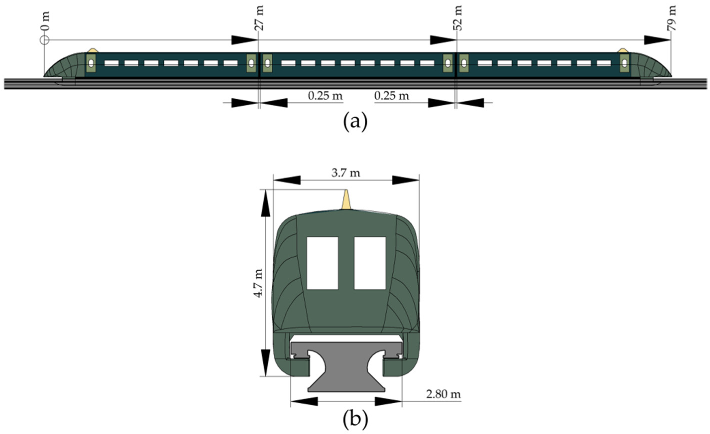
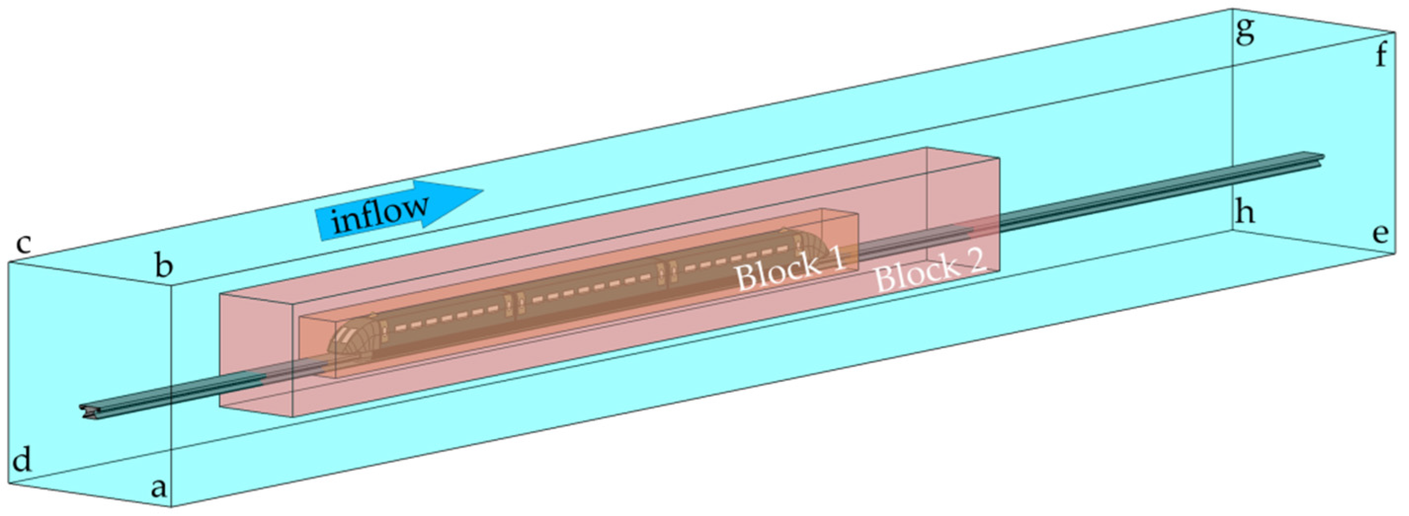
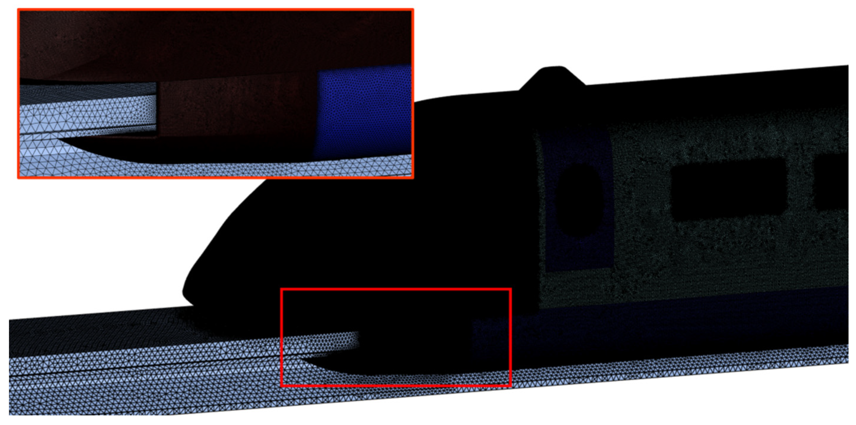
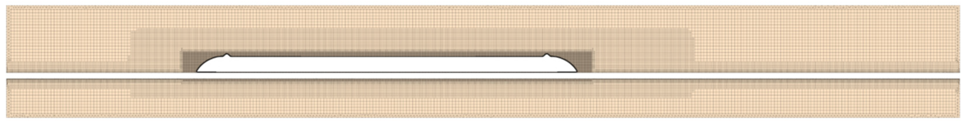
2.1. Numerical Simulation Model of the Flow Field

The three-dimensional and triple-unit configuration of the Shanghai TR08 Maglev system exhibits longitudinal dimensions of 27 m for both terminal vehicular modules and 24.5 m for the intermediate coach section, with 0.25 m windshield clearance between adjacent units, culminating in an aggregate length of 79 m for the complete train formation, as shown in Figure 1a. Geometric abstraction was used to solve the inherent surface irregularity problem in the geometry, and smaller auxiliary features were excluded from the computational domain. Vertical clearance and lateral span measurements were 4.7 and 3.7 m, respectively, while the transverse deck dimension of the guideway was 2.8 m, as shown in Figure 1b. The electromagnetic suspension maintained a 10 mm operational clearance above the elevated bridge structure, with a 10 m vertical elevation [16]. This streamlined topology modeled using SolidWorks is shown in Figure 1.
The fluid dynamics simulation domain encompassing the full-scale Maglev vehicle configuration on the guideway system is shown in Figure 2. The spatial arrangement comprised a 40 m inflow boundary offset from the leading vehicle nose and an 80 m outflow boundary clearance from the trailing vehicle nose, yielding a 199 m longitudinal computational span. Vertically, the domain extended 10 m below and 13.5 m above the guideway reference plane, establishing a total vertical dimension of 23.5 m. The lateral confinement of the domain measured 22.2 m in the transverse direction.
The aerodynamic simulation framework incorporated compressible flow considerations for Maglev velocities of 235, 300, and 430 km/h. The abcd boundary was configured as a pressure far-field with 1 atm pressure and a zero yaw angle. Symmetric constraints were applied to the aefb, bfgc, and cghd planes. Ground effect modeling utilized slip walls on aehd and guideway surfaces with velocities matching the inflows. The train surface was defined as a no-slip stationary wall. The efgh boundary implemented a pressure outlet at ambient conditions. Two mesh refinement zones (Blocks 1 and 2) were strategically positioned around the train geometry to ensure computational accuracy, as shown in Figure 2.
The computational framework employed a hybrid meshing strategy with refinement zones to achieve the required solution accuracy. The mesh partitioned using Fluent Meshing is shown in Figure 3. Surface discretization followed curvature-adaptive principles where grid element dimensions scaled inversely with surface curvature gradients. Critical flow resolution parameters were defined through simultaneous resolution of boundary layer dynamics and turbulence modeling requirements. Specific element sizing included 10 mm for aerodynamically sensitive zones (streamlined nose/tail sections), 30 mm for geometrically stable regions (door interfaces, carriage junctions, and underbody components), and 100 mm for guideway surfaces. The final surface grid configuration contained approximately 22 million elements.
The near-body flow region was discretized using unstructured prismatic elements to accommodate complex geometries. A wall-resolved large eddy simulation (LES) approach was implemented with the first grid node placement at 0.01 mm normal to the solid surfaces. The boundary layer transition was achieved through 25 progressively expanding prismatic layers (growth factor 1.05), ensuring a smooth velocity gradient resolution between the viscous sublayer and main flow regions.
The meshing strategy employed dual refinement blocks to enhance the flow-resolution accuracy. Block 1 enveloped the Maglev train surfaces with a maximum element size of 100 mm, while Block 2 had a 300 mm mesh control to mitigate wake interference. Transitional mesh layers bridged prismatic boundary elements with hexahedral core grids, maintaining global element dimensions <500 mm. The final volumetric grid configuration contained approximately 255 million elements, with the mesh topology of the symmetry plane shown in Figure 4.
A dual-phase computational strategy implemented in ANSYS Fluent ensured numerical stability in the transient flow analysis. Initial steady-state simulations (3000 iterations) employed compressible shear stress transport (SST) k-ω turbulence modeling [17], solved via a semi-implicit pressure-linked equations (SIMPLE) algorithm with second-order upwind discretization for momentum/turbulence parameters. Converged steady-state solutions provided initial conditions for transient LES computations utilizing the wall-adapting local eddy (WALE) sub-grid model. Temporal discretization adopted a bounded second-order implicit schemes, while spatial terms used central differencing for momentum with standard pressure-velocity coupling.
A two-stage temporal resolution strategy was implemented for the flow field evolution analysis. The initial phase employed a timestep of 1 × 10⁻⁴ s to advance the solution to 0.1 s, ensuring turbulent flow development. Subsequently, the temporal resolution was enhanced to 5 × 10⁻⁵ s with full-field data archiving per timestep, extending the simulation to 0.2 s for capturing detailed vortex dynamics.

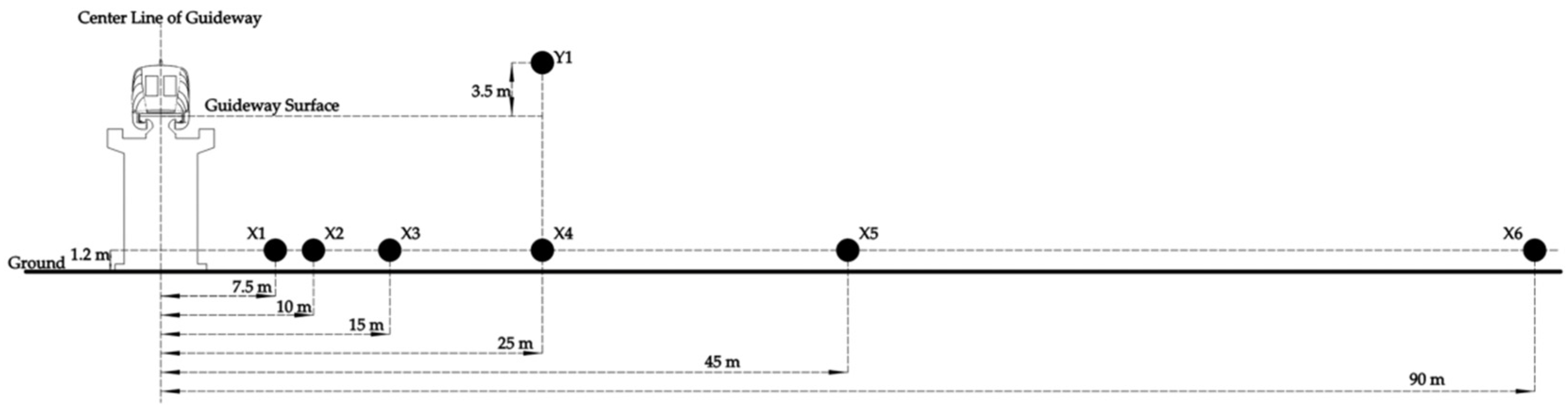
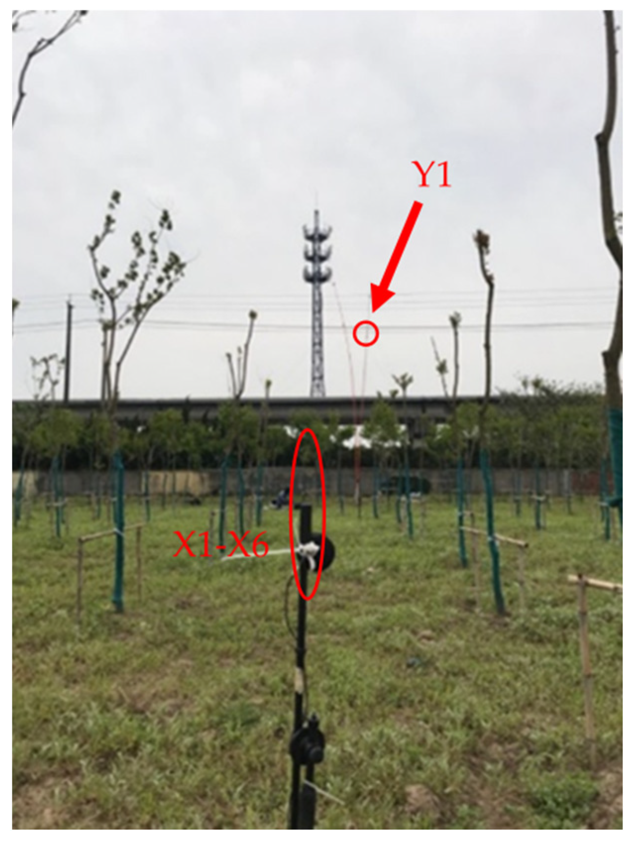
2.2. On-Track Experiment

Measurements were obtained under naturally occurring conditions characterized by ambient wind speeds <1.5 m/s and background noise levels <60 dB. Operational velocities spanning 230–430 km/h at a zero yaw angle were systematically evaluated. Figure 5 shows the acoustic measurement array configuration for pass-by noise characterization.
The height of measuring points X1–X6 above the ground was 1.2 m, and the horizontal distances of X1–X6 from the center line of the guideway were 7.5, 10, 15, 25, 45, and 90 m, respectively. The horizontal distance of measuring point Y1 from the centerline of the guideway was 25 m, and the height of the guideway surface was 3.5 m. Referring to the international standard ISO3095-2013, this measuring point is called the noise standard point [18]. All microphones were in the same cross-section perpendicular to the guideway, and the on-site pass-by noise testing setup is shown in Figure 6.
The experimental setup incorporated Brüel & Kjær LAN-XI hardware with PULSE LabShop software, operating at a 65.5 kHz sampling rate across a 0–25.6 kHz frequency range. This configuration supported extended-duration signal acquisition while performing fast Fourier transform (FFT) and constant percentage bandwidth (CPB) analyses.

2.3. Analysis of Simulation and Experimental Results

Figure 7 compares the time-domain curves of the pass-by noise at measuring point Y1 at different train operating speeds, the vertical axis denotes the A-weighted fast time weighted sound pressure level LA,F. During the passage of the Maglev train, the LA,F initially exhibited a rapid increase and maintained relative stability over a brief duration, followed by a gradual decrease, with the curve demonstrating asymmetric characteristics.
Figure 8 shows the equivalent continuous A-weighted SPL LAeq,T variation curves in logarithmic coordinates with lateral distance at measurement points X1–X6 at different train operating speeds. The LAeq,T continuously decreased with increasing lateral distance, with essentially consistent attenuation patterns across all tested speeds. A strong linear relationship was observed between the LAeq,T and logarithm of the lateral distance. The fitted curves for each train operating speed exhibited coefficients of determination >0.99, with attenuation coefficients ranging from 12.3 to 14.8 dB/log10(m). The measured sound level reduction per distance doubling reached 3.7–4.5 dB(A), indicating that the external noise radiation characteristics of the Maglev train correspond to those of an incoherent line source.
Figure 9 shows the numerically simulated three-dimensional vortex structures visualized using the velocity-colored Q-criterion around the Maglev train operating at 430 km/h. The results reveal that (1) vortex formation occurred at the high-pressure zone of the leading train owing to premature airflow separation; (2) the streamlined profiles induced flow separation at both the head and tail sections, generating distinct detached vortex structures downstream; and (3) a pair of counter-rotating wake vortices developed at the tail section, evolving into stable trailing vortex structures during downstream propagation. With increasing train operating speed, the vortex distribution demonstrated enhanced spatial complexity, exhibiting larger spanwise/vertical scales of vortex pairs, which expanded the effective noise source distribution range. Therefore, regions with intense turbulent movement were taken as strong noise sources. As shown in Figure 9, the positive-pressure area in front of the train, the streamline part of the head, the middle part of the train, the streamline part of the tail, and the negative-pressure area in the rear of the train were divided into five parts: l1, l2, l3, l4, and l5.

3. Construction of the Noise Prediction Model

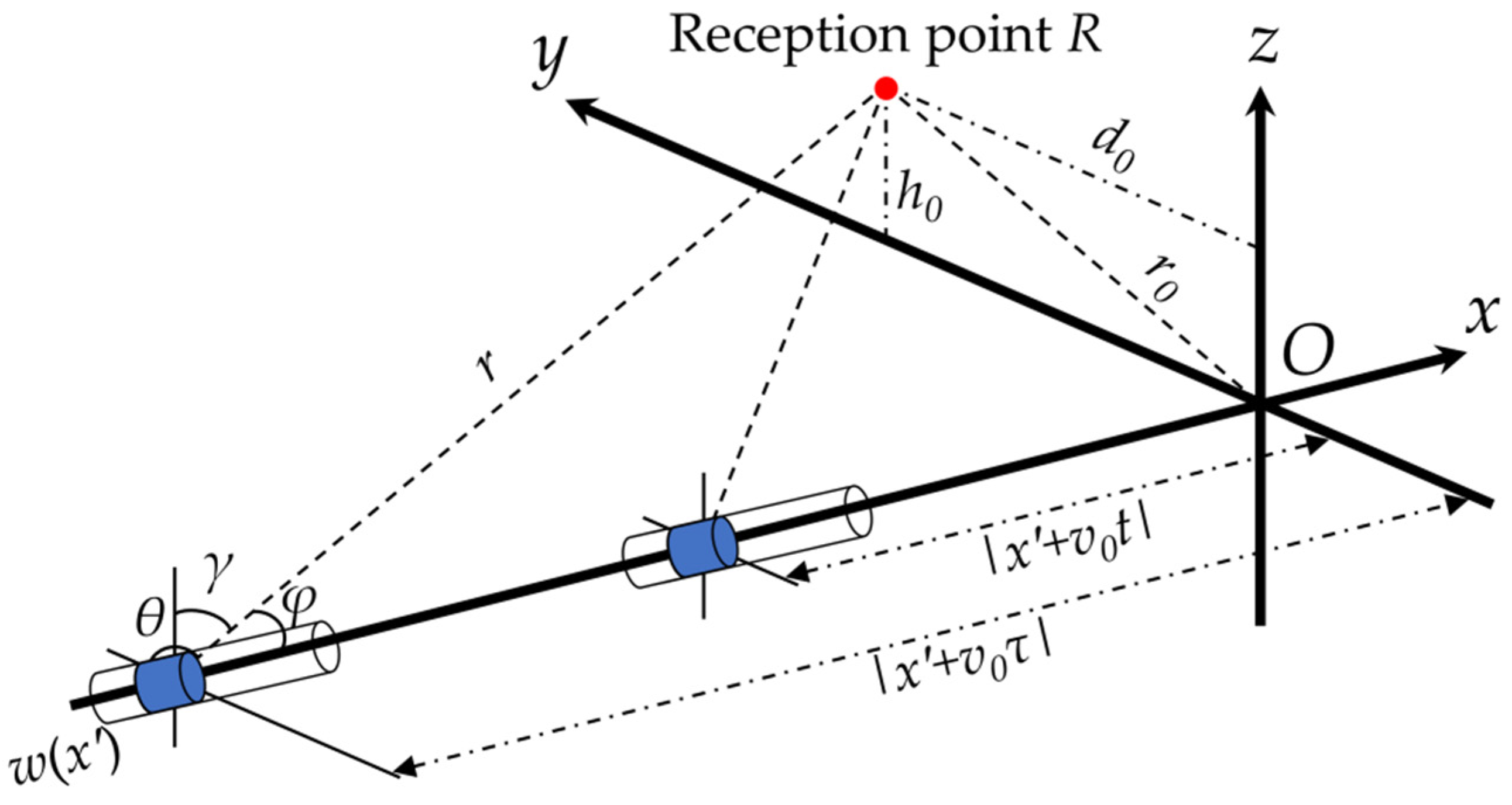
3.1. Finite-Length Incoherent Moving Line Source Model

Figure 10 provides a schematic of the acoustic radiation from a finite-length moving line source within the global coordinate system O-xyz. The line source moves along the positive x-axis at velocity v0, with the reception point R located at global coordinates (0, d0, h0) and maintaining a perpendicular distance r0 from the source axis. The blue cylinder represents the infinitesimal element of a line source; its coordinates are (x′, 0, 0), and the radiated acoustic power is w(x′)dx′. τ is the moment at which the line source element emits sound waves, t is the moment at which R receives the sound waves emitted by the line source element at time τ, and the center of the line source moves exactly to point O at time t = 0. The spatial global x-axis coordinates of the element at times τ and t are x′ + v0τ and x′ + v0t, respectively. The distance between the element and R is r, and the angles between the lines from the element to R and the x-, y-, and z-axes are φ, θ, and γ, respectively.
r is the distance that the sound wave travels at the sound speed c0, which can be expressed as
r = c 0 ( t τ ) = ( x + v 0 τ ) 2 + r 0 2
After squaring Equation (1), it can be arranged into a quadratic equation about τ:
( 1 M 0 2 ) τ 2 2 t + M 0 x c 0 τ + t 2 x 2 + r 0 2 c 0 2 = 0 ,
where the Mach number M0 = v0/c0 < 1, and the following solution for τ can be obtained:
τ = M 0 x + c 0 t ± ( x + v 0 t ) 2 + ( 1 M 0 2 ) r 0 2 c 0 ( 1 M 0 2 ) .
Substituting the above formula into Equation (1) obtains
r = c 0 ( t τ ) = M 0 ( x + v 0 t ) ( x + v 0 t ) 2 + ( 1 M 0 2 ) r 0 2 1 M 0 2 .
As ( x + v 0 t ) 2 + ( 1 M 0 2 ) r 0 2 > x + v 0 t > M 0 ( x + v 0 t ) , r is always greater than 0 when a positive sign is taken before the root of the upper formula, and r is always less than 0 when a negative sign is taken. As r is a distance, it only has meaning when r is a positive real number and a positive sign is taken before the root of the upper formula. If the directivity of the sound source is not considered, the square of the sound pressure generated by the sound wave emitted by the microelement propagating to R in the free field is [19,20]
d p 2 = ρ c 0 w ( x ) 4 π r ( x ) 2 d x = ρ c 0 w ( x ) ( 1 M 0 2 ) 2 4 π ( x + v 0 t ) 2 + ( 1 M 0 2 ) r 0 2 M 0 ( x + v 0 t ) 2 d x .
When a Maglev train runs at high speed, the fluid on the boundary is subjected to pulsating pressure on the surface of the car body, and the pulse power source can be regarded as a dipole sound source whose dipole moment direction is consistent with the side normal direction of the car body. If a line source element is considered to have dipole directivity, then the square of the sound pressure propagated by the sound wave emitted by the element to reception point R can be expressed as
d p 2 = ρ c 0 w ( x ) cos 2 θ 4 π r ( x ) 2 d x = ρ c 0 d 0 2 w ( x ) 4 π r ( x ) 4 d x ,
where cos θ = d 0 / r . Without the loss of generality, the directivity factor of d p 2 can be expressed as cos 2 m θ , and m values of 0, 0.5, and 1, respectively, yield the directivity of no direction, intermediate directivity, and dipole directivity. Then, the square of the sound pressure of the sound wave propagated by the element to R is
d p 2 = ρ c 0 w ( x ) cos 2 m θ 4 π r ( x ) 2 d x = ρ c 0 d 0 2 m w ( x ) 4 π r ( x ) 2 + 2 m d x .
If the sound source is a uniform and incoherent line source, then the square of the sound pressure at R at time t is the linear superposition [21] of the squares of the sound pressures when the sound waves emitted by each element reach the receiving point at time t, so the SPL at R at time t can be expressed as
S P L ( t ) = 10 log 10 p ( t ) 2 / p r e f 2 = 10 log 10 l / 2 l / 2 ρ c 0 w d 0 2 m ( 1 M 0 2 ) 2 + 2 m 4 π p r e f 2 ( x + v 0 t ) 2 + ( 1 M 0 2 ) r 0 2 M 0 ( x + v 0 t ) 2 + 2 m d x ,
where p r e f is the reference sound pressure, with a value of 20 μPa, and l is the length of the line source. A moving object causes a stress change in the surrounding fluid, which can be regarded as a pair of equal and opposite dipoles acting on the same spatial position, that is, a quadrupole sound source. If the linear sound source element is considered to have equiaxial quadrupole directivity and the plane formed by a pair of dipoles that make up the quadrupole is parallel to the y–z plane, then the square of the sound pressure propagated by the sound wave emitted by the element to the reception point can be expressed as
d p 2 = ρ c 0 w ( x ) cos 2 θ cos 2 γ 4 π r ( x ) 2 d x = ρ c 0 h 0 2 d 0 2 w ( x ) 4 π r ( x ) 6 d x .
Similarly, the SPL at the reception point at time t can be expressed as
S P L ( t ) = 10 log 10 p ( t ) 2 / p r e f 2 = 10 log 10 l / 2 l / 2 ρ c 0 w h 0 2 d 0 2 ( 1 M 0 2 ) 6 4 π p r e f 2 ( x + v 0 t ) 2 + ( 1 M 0 2 ) r 0 2 M 0 ( x + v 0 t ) 6 d x

3.2. Equivalent Source Strength

Based on the simulation results of the flow field described in Section 2.3, the exterior noise prediction of the high-speed Maglev train was implemented using a five-segment incoherent line source equivalent model. The sound sources were equivalently modeled as finite-length incoherent line sources with intermediate directivity, where the sound power levels Lw1, Lw2, Lw3, Lw4, and Lw5 correspond to the front positive-pressure zone, streamlined head section, middle carriage section, streamlined tail section, and rear negative-pressure zone, respectively. Computational validation confirmed the optimal positioning of line source segments at the rail level (0 m height) on the vehicle side, with the horizontal distance between R and the vehicle side defined as d. Figure 11 provides a schematic of the equivalent acoustic source model for the high-speed Maglev train noise prediction.
Reference standards ISO 3095-2013 [18] and HJ 2.4-2021 [11] define the position 25 m from the centerline of the guideway and 3.5 m above the guideway surface as the reference measurement point of the source intensity. The equivalent continuous A-weighted sound level during the train passing time at this position is called the noise source intensity. When sound sources S1S5 act alone, the noise source intensity is Lp1Lp5. As the noise source intensity obtained in a real train test is the result of the joint action of all sound sources, to improve the accuracy of the environmental noise prediction model of the Maglev train, Lp1Lp5 should be separated.
According to Equation (8), the SPL at the reception point generated by the combined effect of five uniform finite-length line source segments with intermediate directivity is expressed as
L p ( t ) = 10 log 10 d ( 1 M 0 2 ) 3 4 π + 10 log 10 v 0 t L 2 v 0 t L 2 + l 1 10 0.1 L w 1 x 2 + ( 1 M 0 2 ) r 1 2 M 0 x 3 d x + v 0 t L 2 + l 1 v 0 t l 3 2 10 0.1 L w 2 x 2 + ( 1 M 0 2 ) r 2 2 M 0 x 3 d x + v 0 t l 3 2 v 0 t + l 3 2 10 0.1 L w 3 x 2 + ( 1 M 0 2 ) r 3 2 M 0 x 3 d x + v 0 t + l 3 2 v 0 t + l 3 2 + l 4 10 0.1 L w 4 x 2 + ( 1 M 0 2 ) r 4 2 M 0 x 3 d x + v 0 t + l 3 2 + l 4 v 0 t + L 2 10 0.1 L w 5 x 2 + ( 1 M 0 2 ) r 5 2 M 0 x 3 d x .
The total length of the five-segment line source is denoted as L, where l1l5 represent the lengths of the line source segments, that is, L = l 1 + l 2 + l 3 + l 4 + l 5 , where l2 = l4 = 7 m, l3 = 65 m, and the sum of the three segments provides a total vehicle length of 79 m. As can be seen from Figure 12, there is a good linear relationship between the length of the line source and the speeds of l1 and l5, where l 1 = 57.15 0.18 v , l 5 = 35.00 + 0.38 v , and v is the train operating speed to be predicted in m/s.
Designating the reference measurement position as R, the instantaneous SPL Lp,R(ti) of the Shanghai Maglev train pass-by noise at R were measured with 0.1 s time intervals based on the full-scale test data from Section 2.2. Using Equation (11), the predicted instantaneous SPL L ~ p,R(ti) at R can be calculated when specific values are assigned to the sound power levels per unit length Lw1Lw5. A least-squares optimization framework was implemented with Lw1Lw5 as the optimization parameters, aiming to minimize the total mean-squared error between the measured and predicted instantaneous SPLs at R.
The optimization process was conducted with three distinct step sizes (10, 1, and 0.1 dB(A)) and corresponding variation ranges (±30, ±10, and ±5 dB(A)) for parameter adjustment. By systematically exploring all possible values within the 65–125 dB(A) range, the total mean squared error between the measured and predicted instantaneous SPLs at R was calculated for each combination of parameters. The Lw1Lw5 values that achieved the optimization objective were identified as the optimal sound power levels per unit length. This procedure was repeated for Maglev train operating speeds of 235, 300, and 430 km/h to determine the optimal speed-dependent Lw1Lw5 values, as shown in Table 1.
The optimal values of Lw1Lw5 at different train operating speeds can be used in Equation (11) to calculate the instantaneous SPL at R. As can be seen from Table 2, further calculation results show that the equivalent continuous A-weighted sound level LAeq was obtained during the train passing time, and the absolute error between the measured LAeq,E and predicted LAeq,P values was <0.4 dB(A). These error metrics confirm the high accuracy of the Lw1Lw5 values derived through the least-squares optimization method, validating the effectiveness of the proposed line source model for Maglev train noise prediction across multiple operating speeds. After Lw1Lw5 were solved, according to Equation (11), the noise source intensities Lp1Lp5 when the sound sources S1S5 acted alone were solved.
Figure 13 shows the variation in the sound power levels Lw1Lw5 per unit length of the line sources with train operating speed, where the reference speed vref was 235 km/h. It can be seen from Figure 13 that the sound power levels per unit length of the line sources have a good linear relationship with the normalized velocity logarithm. The prediction formulae for Lw1Lw5 can be expressed as
L w 1 = 69.8 log 10 v v r e f + 76.3 L w 2 = 27.6 log 10 v v r e f + 108.1 L w 3 = 41.0 log 10 v v r e f + 110.2 L w 4 = 35.4 log 10 v v r e f + 111.5 L w 5 = 67.6 log 10 v v r e f + 100.4 ,

3.3. Prediction Model and Parameters

Drawing on the theoretical framework of incoherent finite-line source radiation from Section 3.1, combined with Shanghai Maglev train field measurement data (Section 2.2) and aerodynamic simulation results (Section 2.3), established international methodologies for the exterior noise prediction of high-speed wheel–rail trains and Maglev systems were synthesized to develop an environmental noise prediction model for high-speed Maglev trains. The proposed model employs a five-segment line source equivalence approach, with the equivalent continuous A-weighted sound level LAeq,T at the reception points given by
L A e q , T = 10 log 10 1 T i t e q , i 10 0.1 L p , i + 10 0.1 L b ,
where T is the evaluation time, Lb is the equivalent continuous A-weighted sound level of the background noise at the prediction point, teq,i is the equivalent passing time of train i, and teq,i is calculated as follows:
t e q , i = L v 1 + r 2 / L 2 + r / L ,
where v is the train operating speed to be predicted, in m/s, and r is the distance from the predicted point to the line source. Lp,i is the equivalent continuous A-weighted sound level during passage of the i-th train. The formula is as follows:
L p , i = 10 log 10 10 0.1 L p 1 , i + C i + 10 0.1 L p 2 , i + C i + 10 0.1 L p 3 , i + C i + 10 0.1 L p 4 , i + C i + 10 0.1 L p 5 , i + C i ,
where Lp is the noise source strength of train i at the reference point, which can be obtained from Section 3.2.
C i = C v , i + C d i v , i + C a i r , i + C g , i ,
where Cv,I, Cdiv,I, Cair,I, and Cg,i are the speed correction, geometric divergence correction, air absorption correction, and ground correction of the i-th train, respectively.
For speed correction, according to the fitting formula of the sound power level per unit length of the line source with the running speed, the calculation formula for Cv,i is as follows [11]:
C v , i = 10 log 10 v v r e f ,
where vref is the reference speed, which is 235 km/h.
For the geometric divergence correction, the geometric divergence correction of the i-th train can be expressed as
C d i v , i = 10   log 10 d r 0 3 1 + 1 + L 2 / r 0 2 d 0 r 3 1 + 1 + L 2 / r 2 ,
where d0 and d are the horizontal distances from the strong source reference point and predicted point, respectively, to the side of the car body, and r0 and r are the distances from the strong source reference point and predicted point, respectively, to the sound source.
With air absorption attenuation, sound energy is generated during the heat energy dissipation process owing to the medium viscosity, heat conduction, and molecular relaxation absorption effect of sound waves in air. Sound absorption in air is related to the temperature, humidity, frequency, and propagation distance, and the atmospheric absorption correction of the i-th train can be uniformly expressed as
C a i r , i = α ( r r 0 ) .
In Equation (18), α is the attenuation coefficient of air absorption, and Table 3 presents the attenuation coefficients of air absorption in the octave band under partial temperature and humidity conditions [22]. In general, the sound attenuation caused by air absorption is relatively small, with high-frequency sound waves experiencing greater absorption attenuation than low-frequency sound waves.
The ground correction factors mainly include the correction Cg,r,i caused by ground reflection and ground attenuation correction Cg,a,i caused by interference between direct and reflected sound paths. For the i-th train, the ground correction is expressed as [11]
C g , i = C g , r , i + C g , a , i .
The SPL at R is the result of the superposition of the direct sound and ground-reflected sound energy, and rd and rr are the distances from the sound source S to R and image point R′, respectively. The values of Cg,r,i for smooth, flat, and hard ground are shown in Table 4.
For loose ground or mixed ground that is mostly loose, the ground attenuation correction Cg,a,i is calculated as follows [11]:
C g , a , i = 2 h m / r 17 + 300 / r 4.8
In Equation (20), hm is the average ground height of the propagation path. If Cg,a,i calculated according to Equation (20) is positive, then zero is used to replace Cg,a,i [11].

4. Model Verification and Noise Prediction

To validate the accuracy of the proposed environmental noise prediction model for Maglev trains, a comparative analysis was conducted between the field measurements and model predictions at monitoring points 1.2 m above the ground level along the Shanghai Maglev line. Figure 14 presents time-domain comparisons of the measured and predicted A-weighted fast time weighted sound pressure level LA,F at 45 m from the guideway centerline (1.2 m height) under different train operating speeds. Close alignment was observed between the predicted and measured time-domain trends at 235, 300, and 430 km/h.
The predicted time-domain noise curve of a Maglev train passing at 600 km/h was analyzed at a measurement point located 45 m from the guideway centerline and 1.2 m above ground level. As illustrated in Figure 15, while the temporal characteristics maintained similar trends across different speeds, the 600 km/h speed exhibited significantly sharper peak amplitudes in the waveform compared to those of lower speeds. Furthermore, Figure 15 presents the equivalent continuous A-weighted sound level (LAeq) contributions from individual source intensities (LP1LP5) during train passage at 600 km/h.
Flow field analysis revealed that acoustic energy was primarily concentrated in two critical regions: (1) the near-surface boundary layer along the train body and (2) the wake flow zone downstream of the trailing vehicle. The aerodynamic noise generation mechanisms can be attributed to two dominant flow phenomena: (1) multiple separation vortices along the streamlined shoulder of the leading car, induced by flow separation at the critical geometric transition, and (2) large-scale trailing vortices extending over considerable distances behind the trailing car, resulting from similar flow separation mechanisms at its shoulder region. These observations confirm that vortex-dominated flow structures serve as the primary acoustic sources in high-speed Maglev operations. The intensified vortex dynamics at 600 km/h significantly amplified both peak noise levels compared to lower train operating speeds.
Figure 16 compares the measured and predicted equivalent continuous A-weighted SPL attenuation profiles in logarithmic coordinates during Maglev train pass-by events across multiple speeds as a function of the lateral distance from the guideway centerline (1.2 m height). The experimental and modeled decay trends at identical speeds agree closely, showing consistent distance-dependent attenuation. The cross-speed analysis results reveal maximum absolute deviations of 1.3 dB(A) across all ground-level monitoring points, validating the accuracy of the model while providing extrapolated profiles for 600 km/h operation.

5. Conclusions

In this study, a segmented line source model was developed for predicting the environmental noise distributions of high-speed Maglev trains by integrating uniform finite-length incoherent moving line source (UFL-IMLS) radiation theory with numerical simulations of the external flow field of a Shanghai Maglev train. The key findings are as follows:
(1)
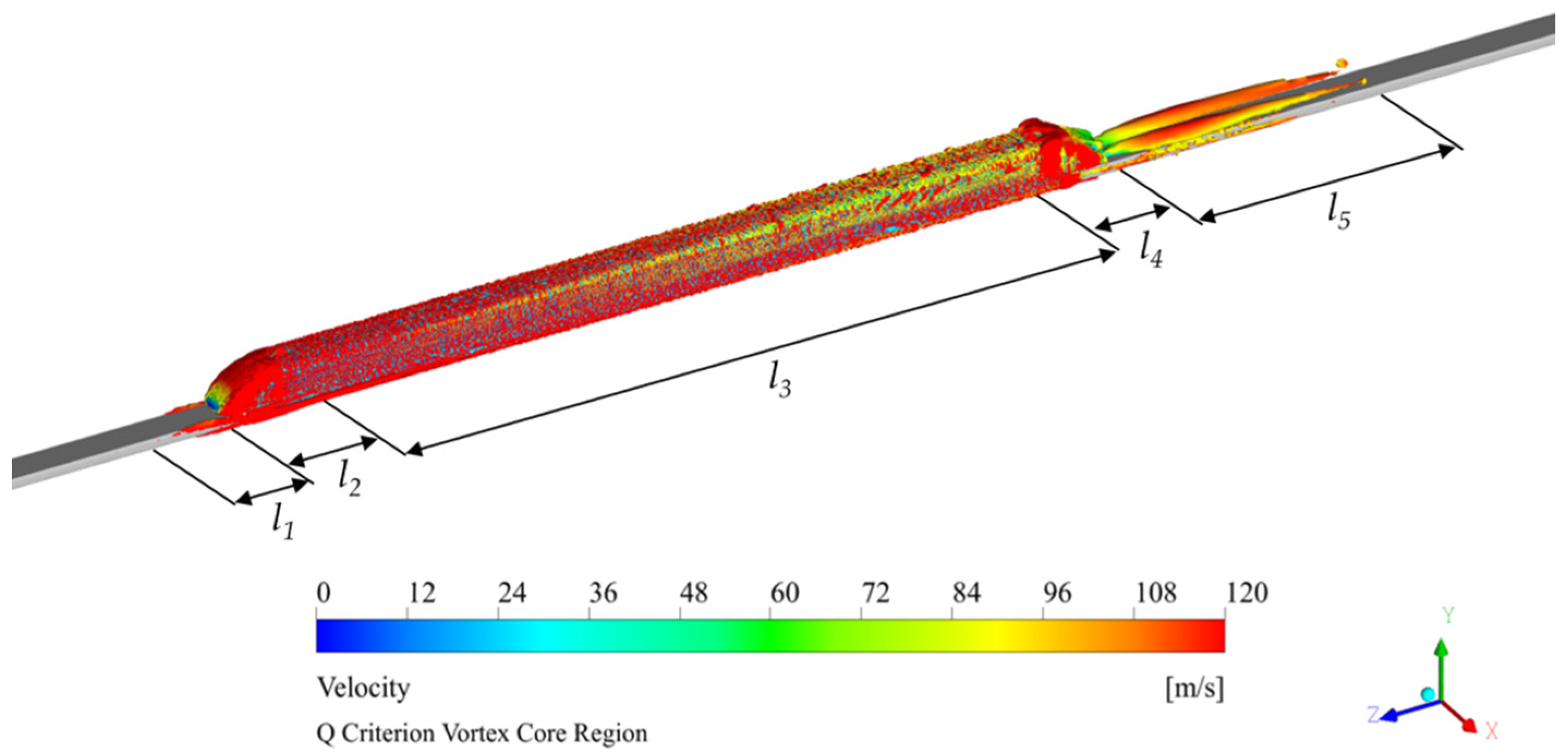
Flow Field Analysis: Incorporating air compressibility effects, the LES method was employed to conduct numerical simulations of the external flow field surrounding a Shanghai Maglev train. The analysis revealed distinct three-dimensional vortical structure distributions with regions of elevated vorticity magnitude concentrated at the vehicle surface and wake zone. Flow separation was observed at the streamlined shoulder of the trailing car, whereas the wake region exhibited a complex array of multiscale vortices with varying intensities, dominated by a pair of counter-rotating ribbon-like trailing vortices. The vortex was the main sound source of fluid flow, and the noise energy was mainly concentrated in the turbulent movement area, such as near the surface of the vehicle body and the wake area. Therefore, the five parts of the turbulent movement around the train were taken as the five-segment line sources.
(2)
Model Validation: The results of a five-segment UFL-IMLS equivalent model derived from the flow simulation data demonstrated strong agreement with the on-site measurements. The maximum absolute deviations in the equivalent sound levels across the monitoring points were constrained to 1.3 dB(A), satisfying the requirements of engineering predictions.
(3)
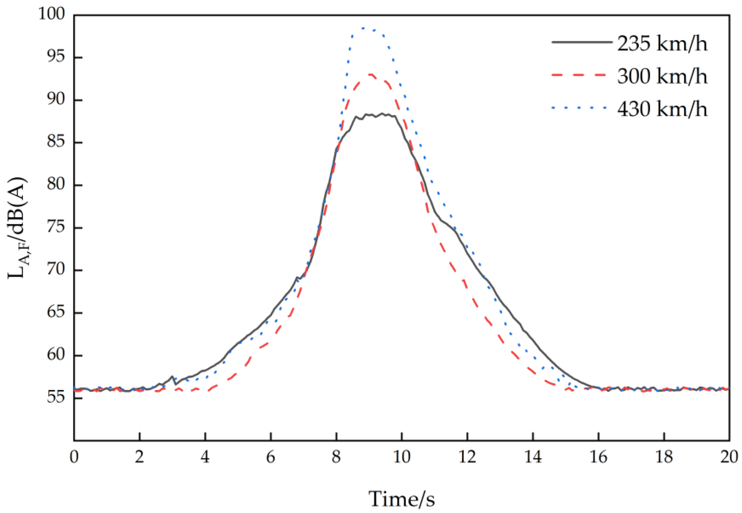
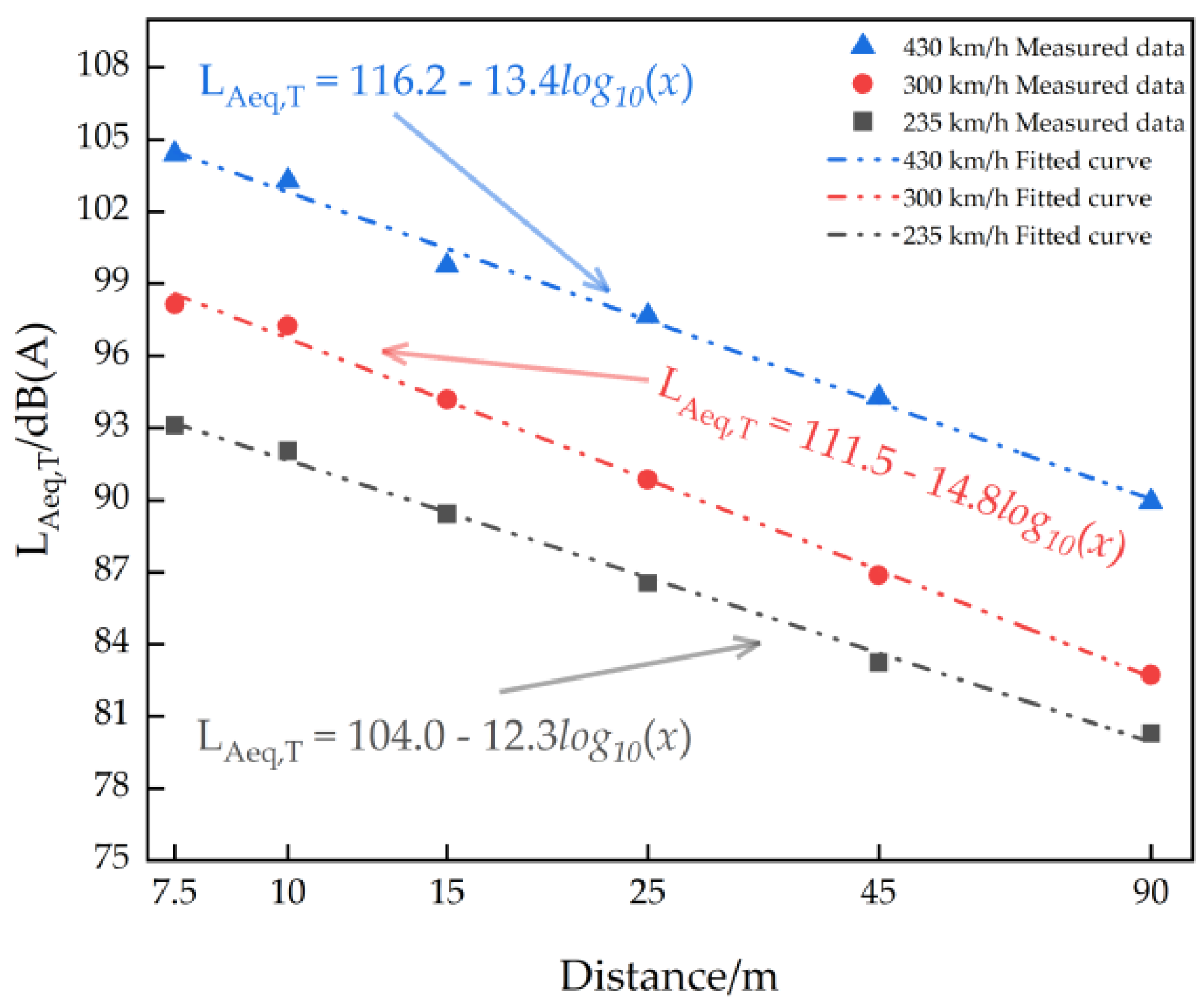
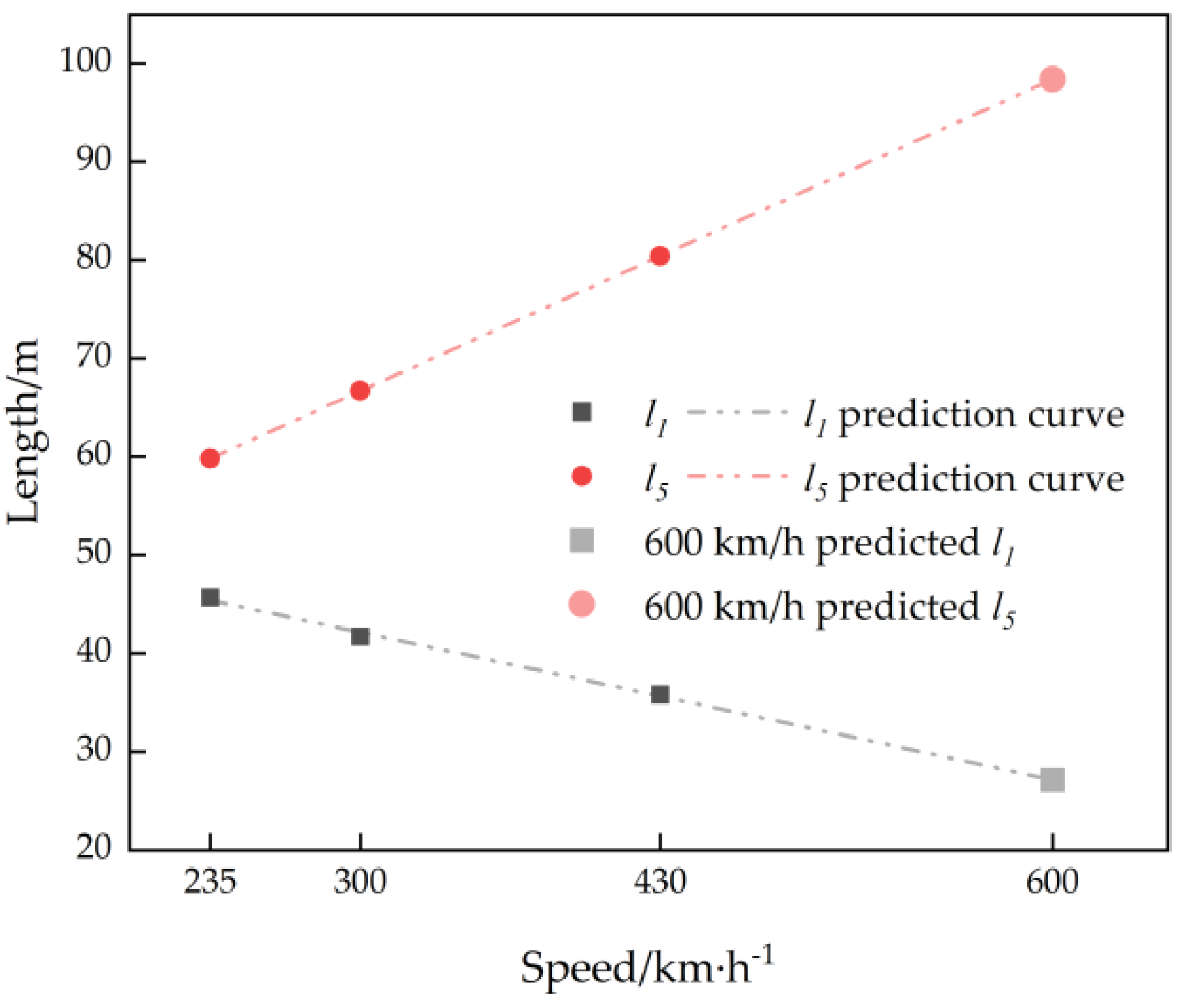
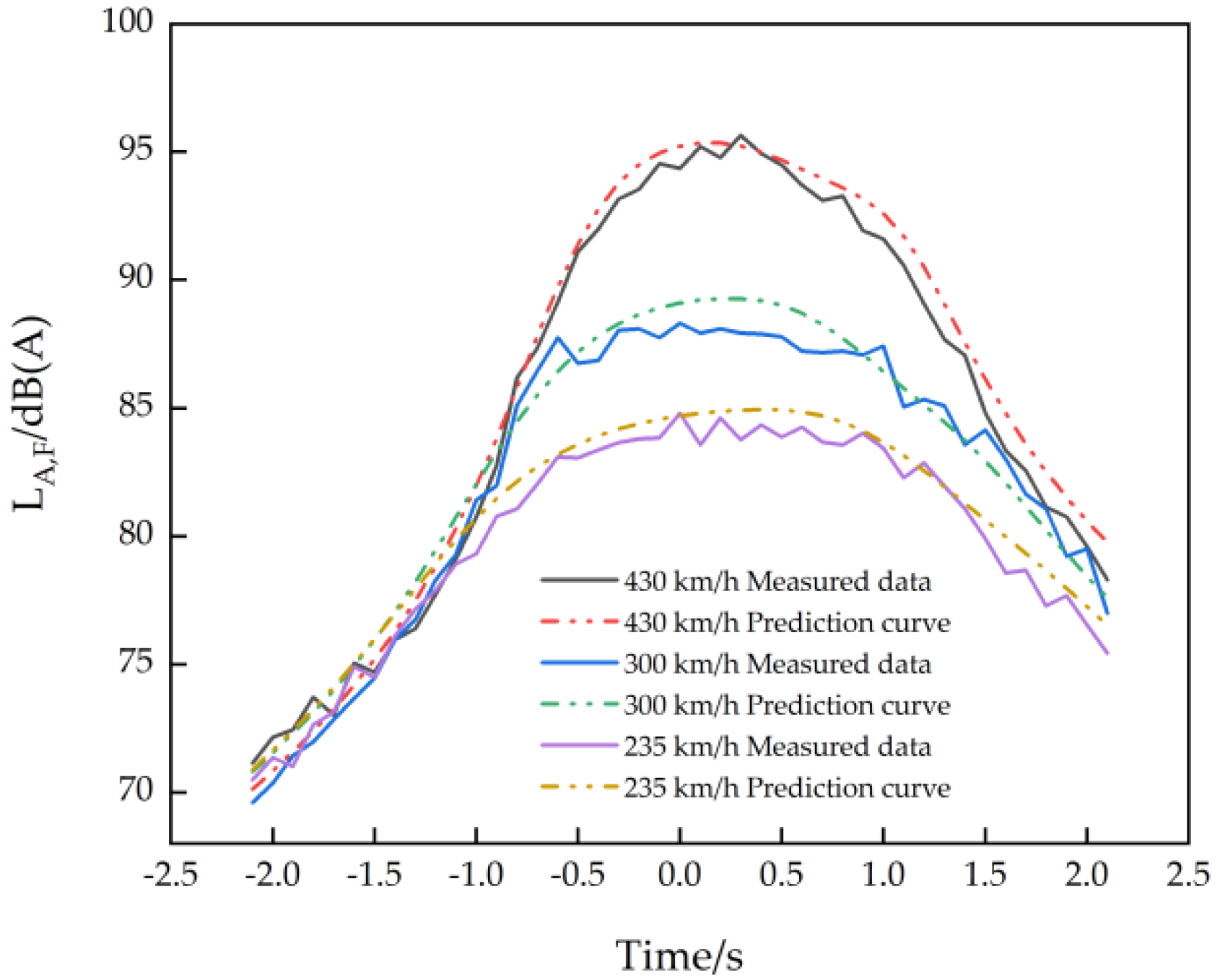
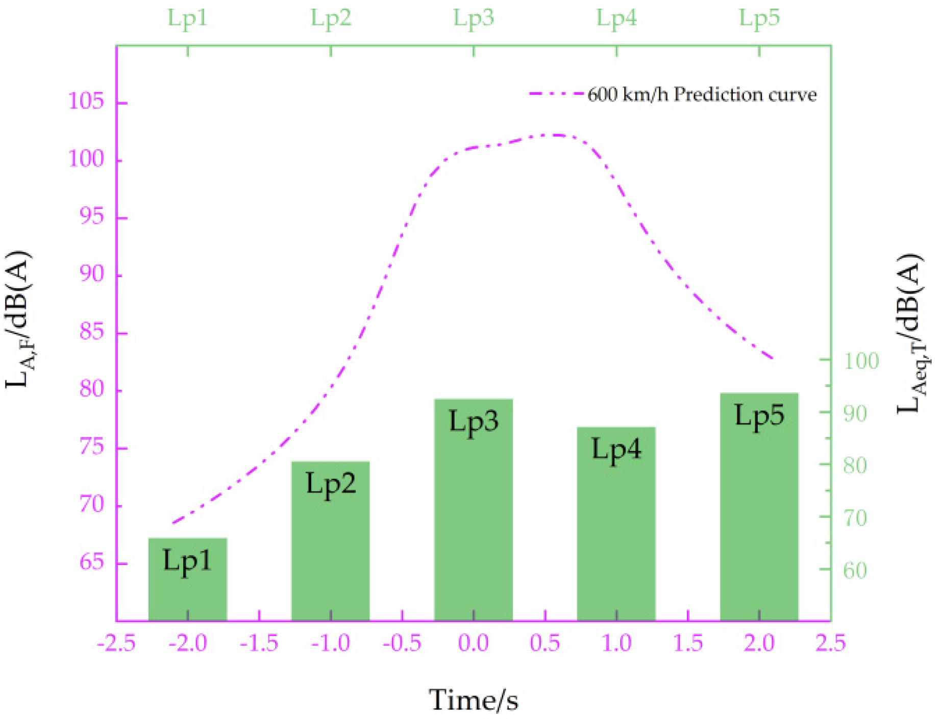
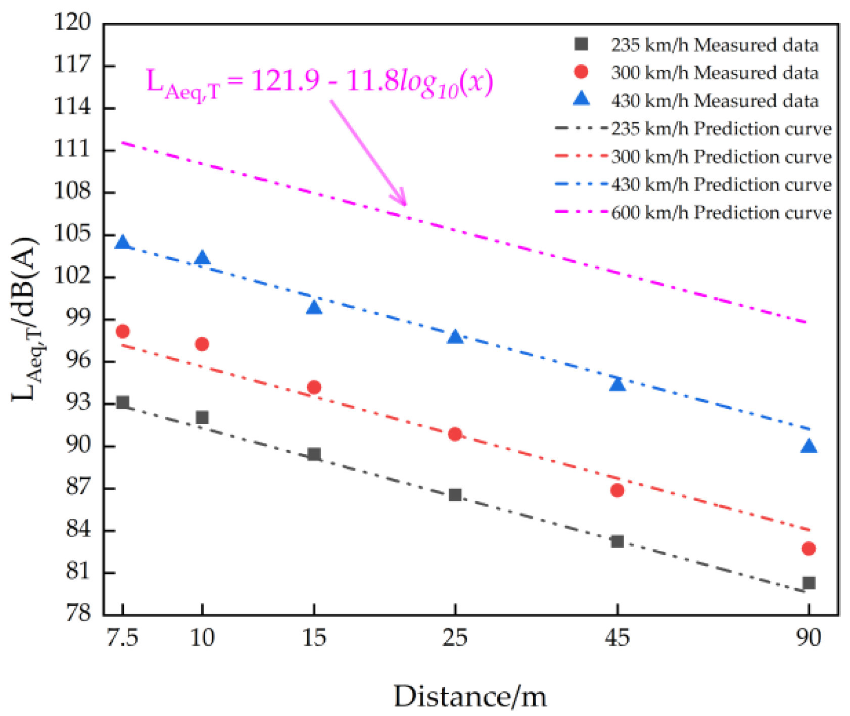
High-Speed Extrapolation: The validated predictions were extended to 600 km/h operation, generating lateral attenuation curves of equivalent continuous A-weighted SPLs and time-domain profiles and providing critical reference information for ultra-high-speed Maglev noise assessment. The time-domain curves of each velocity had similar trends, and the time-domain curve peaks became sharper with an increase in velocity. The curve trends of equivalent continuous A-weighted SPLs with the lateral distance were the same at each speed, and at 600 km/h, the equivalent continuous A-weighted SPLs decreased by 11.8 dB as the logarithm of the lateral distance doubles.

Author Contributions

Conceptualization, S.C.; methodology, S.C.; software, S.C., L.J. and Y.C.; validation, S.C.; formal analysis, L.J.; investigation, L.J.; resources, J.G.; data curation, S.C.; writing the original draft, S.C.; writing, review, and editing, S.C. and J.G.; visualization, S.C. and Y.C.; supervision, J.G.; project administration, J.G.; funding acquisition, J.G. All authors have read and agreed to the published version of the manuscript.

Funding

This research was funded by the Major Strategic Projects of The Chinese Academy of Engineering [grant number: 2018-ZD-16] and CRRC Academy [grant number: 2022CYY004].

Data Availability Statement

The raw data supporting the conclusions of this article will be made available by the authors on request.

Acknowledgments

We gratefully acknowledge Shu Liu (Appraisal Center for Environment & Engineering, Ministry of Ecology and Environment, Beijing) for assistance in securing funding through the Major Strategic Projects of the Chinese Academy of Engineering [grant number: 2018-ZD-16] and Yanju Zhao and Shike Song (CRRC Qingdao Sifang Rolling Stock Research Institute, Qingdao) for their contributions to funding acquisition via the CRRC Academy [grant number: 2022CYY004].

Conflicts of Interest

Author Yuhao Chen was employed by the company CRRC Zhuzhou Times New Material Technology Co., Ltd. The remaining authors declare that the research was conducted in the absence of any commercial or financial relationships that could be construed as a potential conflict of interest.

Abbreviations

The following abbreviations are used in this manuscript:
LESLarge eddy simulation
SELSound exposure level
SPLSound pressure level
UFL-IMLSUniform finite-length incoherent moving line source
SSTShear stress transport
SIMPLESemi-implicit pressure-linked equations
WALEWall-adapting local eddy
FFTFast Fourier transform
CPBConstant percentage bandwidth

References

  1. Prascevic, M.; Gajicki, A.; Mihajlov, D.; Zivkovic, N.; Zivkovic, L. Application of the prediction model “SCHALL 03” for railway noise calculation in Serbia. In Proceedings of the 12th International Symposium Acoustics and Vibration of Mechanical Structures, 23–24 May 2013, Timişoara, Romania; AVMS: Timişoara, Romania, 2013; p. 237. [Google Scholar]
  2. Bundesbahn, D. Richtlinie zur Berechnung der Schallimmissionen von Schienewegen, Schall03/Akustik03; Bundesbahn Zentralamt: München, Germany, 1990.
  3. Moehler, U.; Liepert, M.; Kurze, U.J.; Onnich, H. The New German Prediction Model for Railway Noise “Schall 03 2006”—Potentials of the New Calculation Method for Noise Mitigation of Planned Rail Traffic. In Noise and Vibration Mitigation for Rail Transportation Systems; Notes on Numerical Fluid Mechanics and Multidisciplinary Design; Schulte-Werning, B., Thompson, D., Gautier, P.-E., Hanson, C., Hemsworth, B., Nelson, J., Maeda, T., Vos, P., Eds.; Springer: Berlin/Heidelberg, Germany, 2008; Volume 99, pp. 186–192. [Google Scholar]
  4. Kumar, K.; Bhartia, A.; Mishra, R.K. Monitoring, modeling, and mapping of rail-induced noise at selected stations in megacity Delhi. Int. J. Environ. Sci. Technol. 2023, 20, 10243–10252. [Google Scholar] [CrossRef]
  5. Tsukernikov, I.E.; Tikhomirov, L.A.; Nevenchannaya, T.O. Projected multifunctional hotel complex noise level prediction from railway trains passing (JSC ‘Russian Railways’ connecting branch section) with sound insulation measures development. In IOP Conference Series: Materials Science and Engineering; IOP Publishing Ltd.: Bristol, UK, 2020; Volume 753, p. 022078. [Google Scholar] [CrossRef]
  6. Ivanov, N.I.; Boiko, I.S.; Shashurin, A.E. The problem of high-speed railway noise prediction and reduction. Procedia Eng. 2017, 189, 539–546. [Google Scholar] [CrossRef]
  7. Okada, T. A study on predicting shinkansen noise levels using the sound intensity method. JSME Int. J. Ser. C 2004, 47, 508–511. [Google Scholar] [CrossRef]
  8. Kawahara, M.; Hotta, H.; Hiroe, M.; Kaku, J. Source Identification and Prediction of Shinkansen Noise by Sound Intensity. In Proceedings of the 1997 International Congress on Noise Control Engineering, InterNoise97, Budapest, Hungary, 25–27 August 1997; Institute of Noise Control Engineering: Wakefield, MA, USA, 1997; pp. 151–154. [Google Scholar]
  9. Kanda, H.; Tsuda, H.; Ichikawa, K.; Yoshida, S. Environmental noise reduction of Tokaido Shinkansen and future prospect. In Noise and Vibration Mitigation for Rail Transportation Systems; Schulte-Werning, B., Thompson, D., Gautier, P.E., Hanson, C., Hemsworth, B., Nelson, J., Maeda, T., Vos, P., Eds.; Springer: Berlin/Heidelberg, Germany, 2008; pp. 1–8. [Google Scholar] [CrossRef]
  10. Hanson, C.E.; Ross, J.C.; Towers, D.A. High-Speed Ground Transportation Noise and Vibration Impact Assessment; U.S. Department of Transportation, Federal Railroad Administration, Office of Railroad Development: Washington, DC, USA, 2012.
  11. HJ 453-2018; Technical Guidelines for Environmental Impact Assessment of Urban Rail Transit. Ministry of Ecology and Environment, The People’s Republic of China: Beijing, China, 2018.
  12. Ju, L.; Ge, J.; Guo, Y. Model of high-speed railway noise prediction based on multi-source mode. J. Tongji Univ. (Nat. Sci.) 2017, 45, 58–63. [Google Scholar] [CrossRef]
  13. Brecher, A.; Disk, D.R.; Fugate, D.; Jacobs, W.; Joshi, A.; Kupferman, A.; Mauri, R.; Valihur, P. Noise Characteristics of the Transrapid TR08 Maglev System. 2002. Available online: https://rosap.ntl.bts.gov/view/dot/8507 (accessed on 1 April 2025).
  14. Wang, Z.-S.; Wang, F.-Q.; Gao, S.-Y. Research on Prediction of Noises of High Speed Railway Bridge. J. Southwest Jiaotong Univ. 2001, 14, 166–168. [Google Scholar]
  15. Givargis, S.; Karimi, H. Mathematical, statistical and neural models capable of predicting LA,max for the Tehran–Karaj express train. Appl. Acoust. 2009, 70, 1015–1020. [Google Scholar] [CrossRef]
  16. Cheng, S.; Ge, J.; Zhang, G.; Liu, S. Separation of turbulent pressure and acoustic pressure on a maglev train window and the contribution of interior noise at high speeds. Appl. Acoust. 2025, 231, 110465. [Google Scholar] [CrossRef]
  17. Menter, F.R. Two-equation eddy-viscosity turbulence models for engineering applications. AIAA J. 1994, 32, 1598–1605. [Google Scholar] [CrossRef]
  18. ISO 3095:2013; Acoustics-Railway Applications—Measurement of Noise Emitted by Railbound Vehicles. International Organization for Standardization: Geneva, Switzerland, 2013.
  19. Ffowcs Williams, J.E.; Hawkings, D.L. Sound generation by turbulence and surfaces in arbitrary motion. Philos. Trans. A Math. Phys. Eng. Sci. 1969, 264, 321–342. [Google Scholar]
  20. Ewert, R.; Schröder, W. Acoustic perturbation equations based on flow decomposition via source filtering. J. Comp. Phys. 2003, 188, 365–398. [Google Scholar] [CrossRef]
  21. ISO 3745:2012; Acoustics—Determination of Sound Power Levels and Sound Energy Levels of Noise Sources Using Sound Pressure—Precision Methods for Anechoic Rooms and Hemi-anechoic Room. International Organization for Standardization: Geneva, Switzerland, 2012.
  22. ISO 9613-1:1993; Acoustics, Outdoor Sound Propagation Attenuation Part I: Atmosphere Sound Absorption Calculation. International Organization for Standardization: Geneva, Switzerland, 1993.
  23. Mao, D.; Hong, Z. Environmental Noise Control Engineering; Higher Education Press: Beijing, China, 2010; p. 308. [Google Scholar]
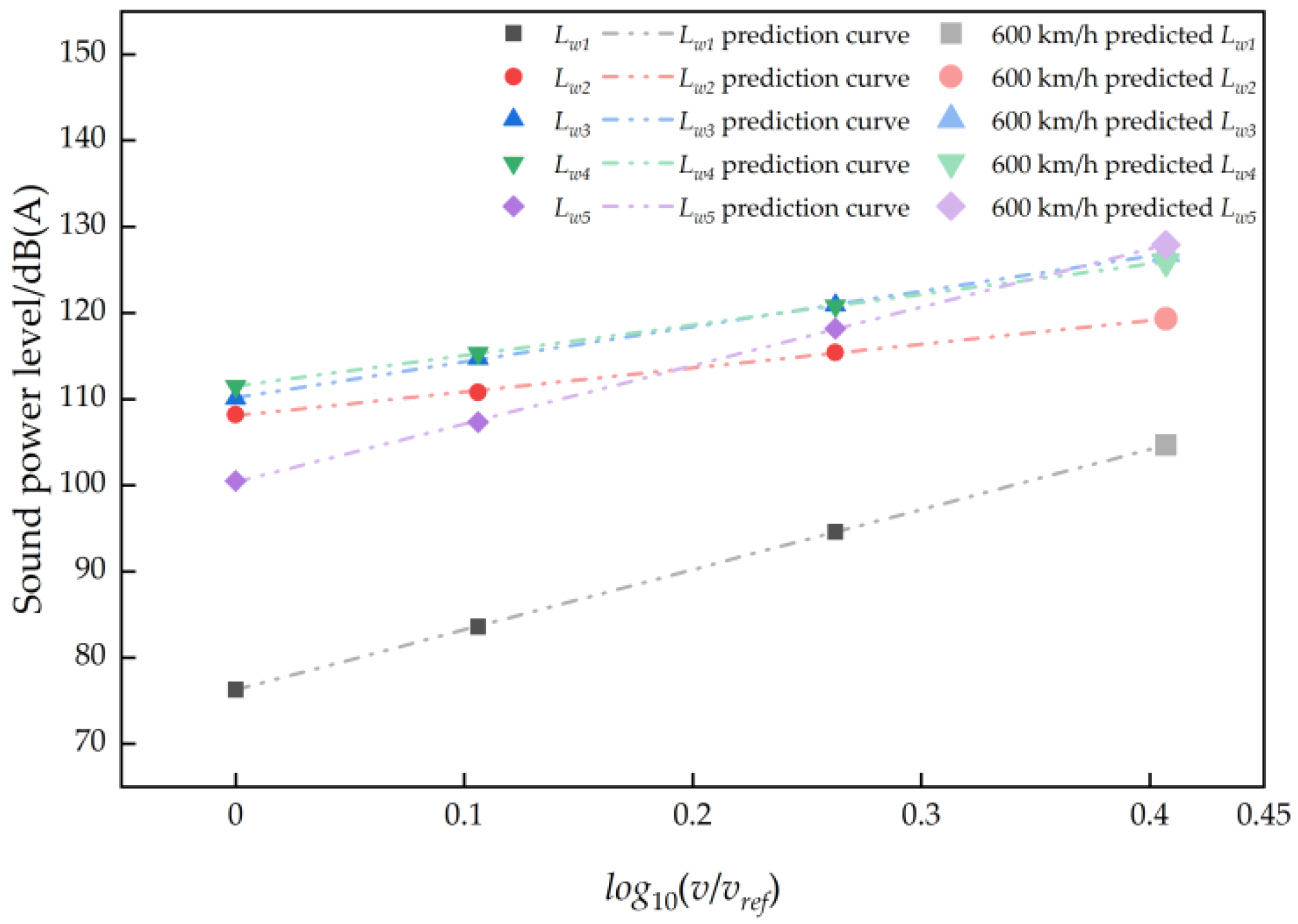
Figure 1. Shanghai Maglev train TR08 geometric model: (a) side view, (b) front view.
Applsci 15 04184 g001
Figure 2. Computational domain and mesh refinement zones.
Applsci 15 04184 g002
Figure 3. Maglev train surface grid.
Applsci 15 04184 g003
Figure 4. Volume mesh topology of the symmetry plane.
Applsci 15 04184 g004
Figure 5. Schematic of external pass-by noise measurement points.
Applsci 15 04184 g005
Figure 6. Photograph of external pass-by noise measurement points.
Applsci 15 04184 g006
Figure 7. Time-domain curves of pass-by noise at point Y1 at different running speeds.
Applsci 15 04184 g007
Figure 8. SPL versus lateral distance at 1.2 m above ground at different running speeds.
Applsci 15 04184 g008
Figure 9. Three-dimensional vortex structures visualized by velocity-colored Q-criterion around the Maglev train at 430 km/h.
Applsci 15 04184 g009
Figure 10. Schematic of acoustic radiation from finite-length moving line sources.
Applsci 15 04184 g010
Figure 11. Schematic of the high-speed Maglev train noise prediction equivalent acoustic source model.
Applsci 15 04184 g011
Figure 12. Line source lengths vary with train operating speed.
Applsci 15 04184 g012
Figure 13. Sound power levels of line sources vary with train operating speed.
Applsci 15 04184 g013
Figure 14. Time-domain comparison of measured and predicted SPLs at 45 m from the guideway centerline (1.2 m above the ground).
Applsci 15 04184 g014
Figure 15. Time-domain prediction curve and LAeq,T when the noise source intensity acted alone at 600 km/h.
Applsci 15 04184 g015
Figure 16. Measured and predicted equivalent continuous A-weighted SPLs as a function of the lateral distance from the guideway centerline (1.2 m above the ground).
Applsci 15 04184 g016
Table 1. Optimal values of Lw1Lw5 at different train operating speeds (dB(A)).
Train Operating Speed (km/h)Lw1Lw2Lw3Lw4Lw5
23576.3108.2110.1111.5100.5
30083.6110.8114.7115.3107.3
43094.6115.4120.9120.8118.2
Table 2. Measured versus predicted SPL errors at different train operating speeds (dB(A)).
Train
Operating Speed
(km/h)
Measured
LAeq,E
Predicted
LAeq,P
LAeq
Error |Δ|
23587.687.90.2
30091.892.20.4
43098.198.60.5
Table 3. Octave-band air absorption attenuation coefficient (units: dB/m).
Temperature
(°C)
Relative
Humidity (%)
Octave-Band Center Frequency (Hz)
125250500100020004000
25503.99 × 10−41.32 × 10−33.23 × 10−35.68 × 10−31.02 × 10−22.57 × 10⁻²
25603.40 × 10−41.18 × 10−33.18 × 10−35.96 × 10−31.02 × 10−22.32 × 10⁻²
25702.96 × 10−41.06 × 10−33.08 × 10−36.19 × 10−31.04 × 10−22.19 × 10⁻²
35602.57 × 10−49.77 × 10−43.32 × 10−38.45 × 10−31.51 × 10−22.58 × 10⁻²
15604.26 × 10−41.18 × 10−32.31 × 10−34.06 × 10−39.5 × 10−33.03 × 10⁻²
0604.01 × 10−47.79 × 10−41.78 × 10−35.50 × 10−31.93 × 10−26.33 × 10⁻²
–10603.60 × 10−49.69 × 10−43.23 × 10−31.09 × 10−22.96 × 10−25.35 × 10⁻²
Table 4. Ground reflection corrections [23] (units: dB(A)).
rr/rd≈1≈1.4≈2>2.5
Cg,r,i3210
Disclaimer/Publisher’s Note: The statements, opinions and data contained in all publications are solely those of the individual author(s) and contributor(s) and not of MDPI and/or the editor(s). MDPI and/or the editor(s) disclaim responsibility for any injury to people or property resulting from any ideas, methods, instructions or products referred to in the content.

