A New Signal Processing Method for Time-of-Flight and Center Frequency Estimation

Abstract

Ultrasonic signal processing methodologies use many signal parameters to be investigated, one of which is time-of-flight (ToF). There are many and various methods used to determine ToF, such as threshold detection, peak-based methods, cross-correlation, zero-crossing tracking algorithms, etc. The application of most of these methods becomes problematic when the background noise becomes high and the signal amplitude, frequency, or propagation velocity changes. In order to partially solve these problems, this paper proposes a new and simple method to determine the time-of-flight and center frequency of signals based on the use of zero-crossing times of filtered signals to calculate these parameters. Taking advantage of the idea that these zero-crossing times are concentrated around the maximum of the signal envelope, they were used as the time-of-flight of the signal. Together with the ToF, the center frequency of the signal was also determined. The proposed method was adapted to the processing of experimental signals obtained during various ultrasound investigations. By processing S₀ mode signals propagating in the sheet molding compound plate, the propagation velocity of this mode was calculated. Its value was compared with the value obtained by the 2D FFT method. The obtained results differed by 0.9%. Using simulated signals propagating in 1 mm-thick aluminum, the phase and group velocity segments of the A₀ mode were calculated. Their values differed by 0.7% from the theoretically calculated values of the dispersion curves by the SAFE method.

1. Introduction

Many fields of scientific research work with various signals that carry important information about the objects being studied. In most cases, these signals are dynamic, i.e., their parameters (amplitude, frequency, propagation time, signal-to-noise ratio, etc.) vary in time and space. Therefore, new or already known signal processing methods are constantly being developed in order to extract as much useful information as possible encoded in the investigated signals.

In recent years, ultrasonic systems using high-speed digital signal processing technologies have made great progress in various fields of measurement and diagnostics. These systems are successfully used for evaluation of mechanical properties of various materials, thickness measurement, determination of chemical composition, temperature evaluation, and defect identification. They are used in gas or liquid flow velocity measurements and biological research. In many of the listed areas, a time-of-flight (ToF) measurement procedure is used.

Ultrasonic signal processing methodologies use many signal parameters to be investigated (amplitude, phase, frequency, group propagation time), one of which is time-of-flight (ToF). There are many and various methods used to determine ToF, such as threshold detection [1,2,3], peak-based methods [4,5,6], cross-correlation [7,8,9,10,11], zero-crossing tracking algorithms [12,13,14], etc. Among these algorithms, the simplest is used to determine the propagation time of the signal based on a threshold of when the signal amplitude exceeds a set level [15]. However, due to the noise level in the signal and the attenuation of the signal, the use of the threshold method is sometimes compromised by the problems of multi-significance and uncertainty. The cross-correlation method has robustness to noise interference and is often used in ToF determination [8]. However, the disadvantage of this method is that the signal must be cross-correlated with the transmitted (reference) signal in order to calculate the ToF. Obtaining a reference signal is difficult in most cases, and the evaluation of the cross-correlation itself is complicated [10]. Zero-crossing algorithms are sensitive to noise, so this method can only be used in a high signal-to-noise ratio (SNR) regime [13].

Recently, time-frequency signal processing methods have become widely used to estimate signal time-of-flight. A new ToF estimation method based on the short-time Fourier transform (STFT) was proposed in [16]. In this method, the time and frequency components of the ultrasound signal are represented by the STFT, and their spectrum is projected into the time domain. The ToF is calculated from the location of the maximum modulus of the signal’s STFT spectrum. The method has many advantages, but the estimation of ToF at signal-to-noise ratio SNR < 8 dB is problematic.

A variety of wavelet-based algorithms, both continuous (CWT) and discrete (DWT) forms, are used to determine the propagation time of signals and reduce noise [17]. In [18], the measured signal was decomposed into a series of narrowband signals using a wavelet transform, and matching pursuit (MP) was used to derive a sparse representation of the signal. In one paper [19], the continuous wavelet transform based on the scale-averaged power (SAP) and the discrete stationary wavelet transform (DSWT) were used. Studies have shown that both methods produce low error for non-overlapping signals and acceptable error for partially overlapping signals. One work [20] describes the broadband wavelet method for time-of-flight measurements of ultrasound pulse echoes. A paper [21] presents the application of the wavelet transform integrated with a threshold detection method. However, the application of most of these methods becomes problematic when the background noise is high and the signal is variable.

In this article, we propose an algorithm for determining the propagation time and center frequency of signals based on the use of zero-crossing times of filtered signals to calculate these parameters. Section 2 describes the methodology used to determine the time-of-flight and center frequency. The processing of different experimental signals by the proposed method is described in Section 3. Section 4 discusses the results of using the method and the limitations of this method.

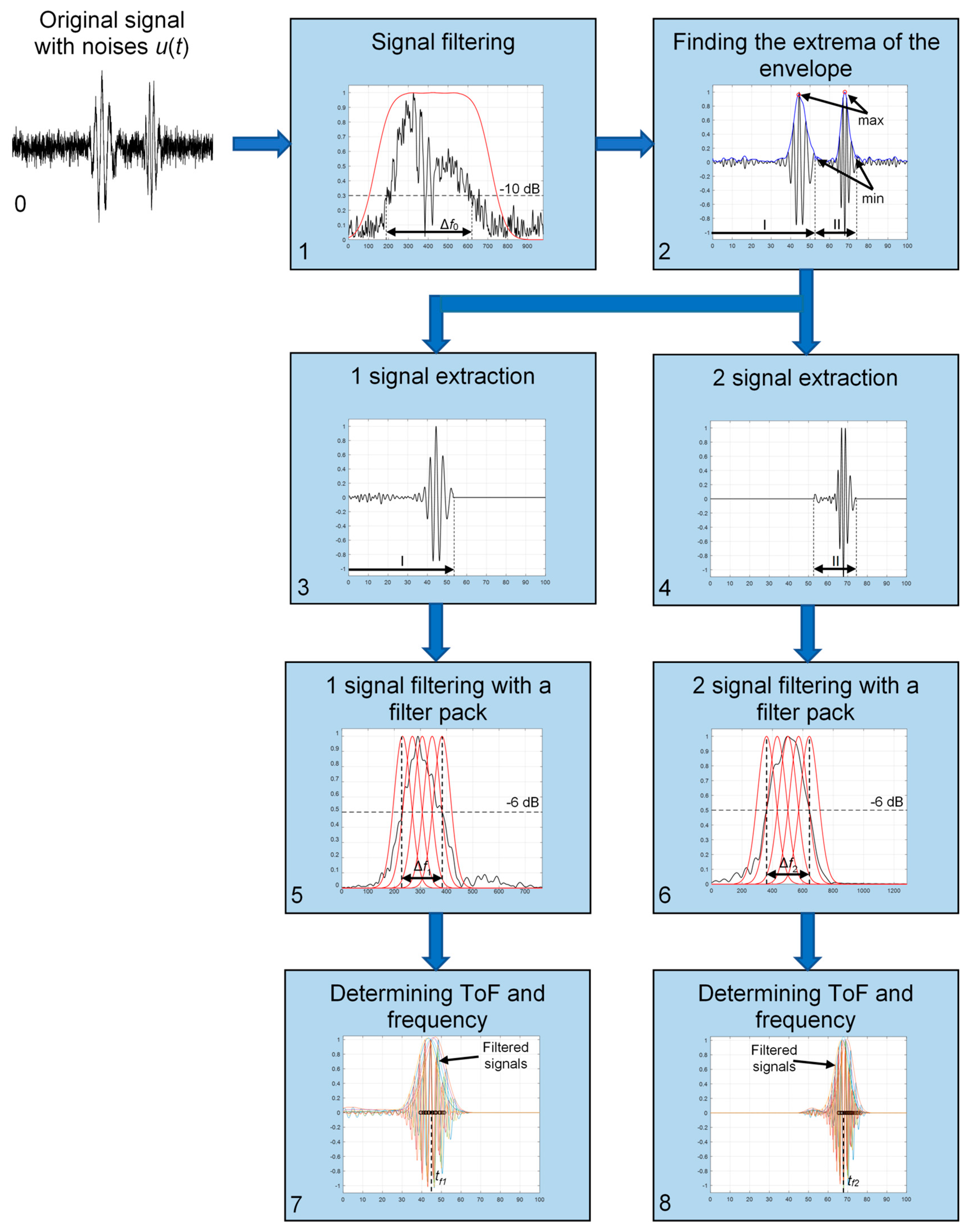
2. Methodology for Estimation of Time-of-Flight and Center Frequency of Signals

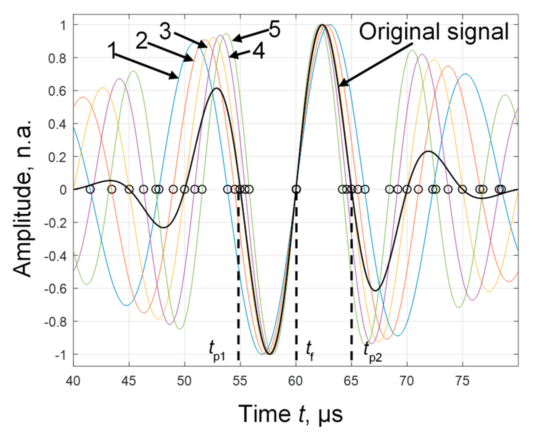
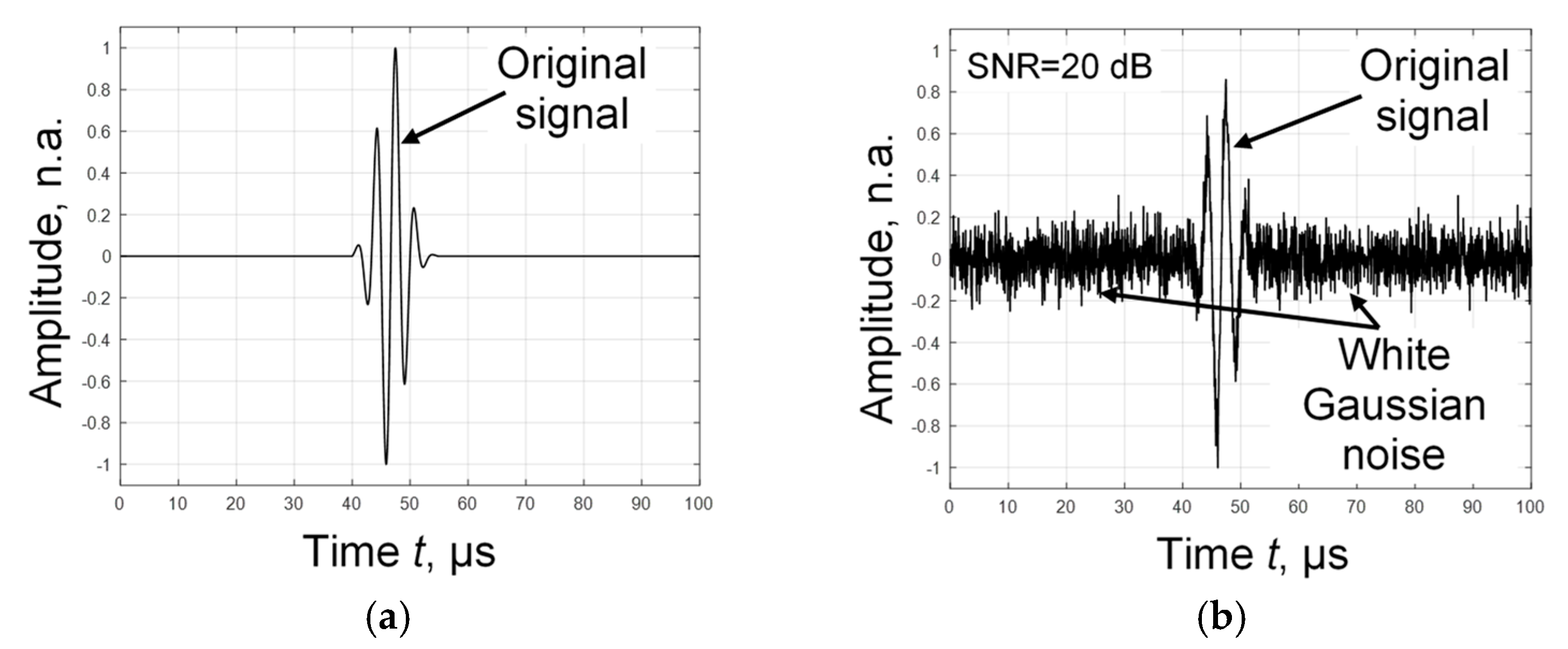
2.1. Signal Processing of Ultrasound Signals with Noises

The measured ultrasonic noisy signal u(t) was a linear combination of the desired clean signal s(t) and the additive noise n(t) [22]. A complex ultrasound signal u(t) was chosen for the explanation of the proposed algorithm. The ultrasonic signal was composed of the sum of two three-period harmonic signals of different center frequencies with a Gaussian envelope (Figure 1, (0))

$$u\left(t\right)=s\left(t\right)+n\left(t\right)=\left\{\begin{array}{c}n\left(t\right),0<t<t_1,\\ A{e}^{-{\displaystyle \frac{t^2}{2s^2}}}\sin \left(2\pi f_{1}t\right)+n\left(t\right),t_1<t<t_2\\ A{e}^{-{\displaystyle \frac{t^2}{2s^2}}}\sin \left(2\pi f_{2}t\right)+n\left(t\right),t_2<t<t_{3,}\end{array}\right.,$$

(1)

where n(t) is the additive white Gaussian noise; A is the signal amplitude, A = 1; s is the pulse width factor; f₁ is the center frequency of the first signal, f₁ = 300 kHz; f₂ is the center frequency of the second signal, f₂ = 500 kHz; t₁ is the delay time of the first signal, t₁ = 40 µs; and t₂ is the delay time of the second signal, t₂ = 65 µs.

Such a signal was chosen with the idea that it would be a complex signal with different frequencies and different time-of-flights.

The initial stage of signal processing is the calculation of its frequency spectra and the determination of its width Δf₀ at the −10 dB level (Figure 1, (1))

$$U\left(f\right)=\mathrm{F}\mathrm{T}\left[u\left(t\right)\right],$$

(2)

$$∆f_0=\max \left(\arg \left\{U\left(f\right)>0.3\right\}\right)-\min \left(\arg \left\{U\left(f\right)>0.3\right\}\right),$$

(3)

where FT is the Fourier transform.

According to the set bandwidth Δf₀, a bandpass filter is formed, the maximum amplitude variation of which covers this bandwidth (Figure 1, (1), red line). Filtering with this filter eliminates part of the spectrum of the noisy signal and highlights the original signal s(t) (Figure 1, (2)). The envelope e(t) of this signal and its extremes (min and max) are determined below

$$e\left(t\right)=\mathrm{H}\mathrm{T}\left[u\left(t\right)\right],$$

(4)

where HT is the Hilbert transform.

Separate signals u₁(t) (Figure 1, (3)) and u₂(t) (Figure 1, (4)) are distinguished with the help of the extremes min₁ and min₂

$$u_1\left(t\right)=u\left(t\right)\mathrm{i}\mathrm{f}t<\arg \left\{{min}_1\left(\mathrm{H}\mathrm{T}\left[u\left(t\right)\right]\right)\right\},$$

(5)

$$u_2\left(t\right)=u\left(t\right)\mathrm{i}\mathrm{f}\arg \left\{{min}_1\left(\mathrm{H}\mathrm{T}\left[u\left(t\right)\right]\right)\right\}<t<\arg \left\{{min}_2\left(\mathrm{H}\mathrm{T}\left[u\left(t\right)\right]\right)\right\}.$$

(6)

where the extreme values “min₁” and “min₂” are the first minimums of the signal envelopes following each maximum of the envelopes (Figure 1, (2)).

Frequency spectra U₁(f) (Figure 1, (5), black line) and U₂(f) (Figure 1, (6), black line) are calculated for the extracted signals.

$$U_1\left(f\right)=\mathrm{F}\mathrm{T}\left[u_1\left(t\right)\right],U_2\left(f\right)=\mathrm{F}\mathrm{T}\left[u_2\left(t\right)\right].$$

(7)

The upper (f_H1 and f_H2) and lower (f_L1 and f_L2) frequency limits at the 6 dB level (0.5 level) are determined by frequency spectra U₁(f) and U₂(f)

$$f_{\mathrm{H}1}=\max \left(\arg \left\{U_1\left(f\right)>0.5\right\}\right),f_{\mathrm{L}1}=\min \left(\arg \left\{U_1\left(f\right)>0.5\right\}\right),$$

(8)

$$f_{\mathrm{H}2}=\max \left(\arg \left\{U_2\left(f\right)>0.5\right\}\right),f_{\mathrm{L}2}=\min \left(\arg \left\{U_2\left(f\right)>0.5\right\}\right),$$

(9)

then the corresponding frequency bands (Figure 1, (5) and (6))

$$∆f_1=f_{H1}-f_{L1},∆f_2=f_{H2}-f_{L2}.$$

(10)

Based on research results [23], we selected a package of five Gaussian filters (Figure 1, (5) and (6), red line) to filter each separated signal u₁(t) and u₂(t)

$$B_{in}(f)=e^{-2.77·{\left({\displaystyle \frac{f-f_{\mathrm{L}n}-(i-1){\mathrm{d}f}_n}{{∆B}_n}}\right)}^2},$$

(11)

$$g_{i1}\left(t\right)={\displaystyle \frac{1}{2\pi }}{\int }_{-\mathrm{\infty }}^{\mathrm{\infty }}\mathrm{F}\mathrm{T}\left(u_1\left(t\right)\right)B_{i1}\left(\omega \right)e^{j\omega t}d\omega ,$$

(12)

$$g_{i2}\left(t\right)={\displaystyle \frac{1}{2\pi }}{\int }_{-\mathrm{\infty }}^{\mathrm{\infty }}\mathrm{F}\mathrm{T}\left(u_2\left(t\right)\right)B_{i2}\left(\omega \right)e^{j\omega t}d\omega ,$$

(13)

where B_in(f) is the frequency response of i-th bandpass filter, i = 1–5, n—number of separated signal, ${df}_n={\displaystyle \frac{f_{\mathrm{H}n}-f_{\mathrm{L}n}}{4}}$ are the steps between central frequencies of two neighboring filters, and ΔB_n are the bandwidths of the filters. The bandwidths of the filters were chosen from the Δf_n/ΔB_n = 2.5 condition [23].

Next, in each filtered signal, the zero-crossings of the signals are identified (Figure 2):

$$t_{\mathrm{e}\mathrm{m}\mathrm{a}\mathrm{x}n}=\mathrm{a}\mathrm{r}\mathrm{g}\left\{\mathrm{m}\mathrm{a}\mathrm{x}\left(e_n\left(t\right)\right)\right\},$$

(14)

$$t_{ikn}^0=\mathrm{a}\mathrm{r}\mathrm{g}\left\{g_{in}\left(t\right)\cong 0\right\},\mathrm{if}{t}_{\mathrm{e}\mathrm{m}\mathrm{a}\mathrm{x}n}-{\displaystyle \frac{5}{{2f}_{in}}}<t<t_{\mathrm{e}\mathrm{m}\mathrm{a}\mathrm{x}n}+{\displaystyle \frac{5}{2f_{in}}},$$

(15)

where $t_{ikn}^0$ are the zero-crossings of i-th filter, k = 1, 2, … K is the number of zero-crossings, K is the total number of zero-crossings, f_in is the central frequency of i-th filter.

Finally, the ToF of the separated signals t_f1 (Figure 1, (7)) and t_f2 (Figure 1, (8)) are determined by averaging the times of the concentrated zero-crossings instances $t_{i\mathrm{M}n}^0$

$$t_{i\mathrm{M}n}^0=\mathrm{a}\mathrm{r}\mathrm{g}\left\{\mathrm{m}\mathrm{i}\mathrm{n}\left({\sum }_{i=1}^4\left(\underset{1<k<\mathrm{K}}{\min }\left(t_{ikn}^0-t_{(i+1)kn}^0\right)\right)\right)\right\},$$

(16)

$$t_{fn}={\displaystyle \frac{1}{5}}{\sum }_{i=1}^5{t}_{i\mathrm{M}n}^0,$$

(17)

where M is the number of zero-crossings in the i-th filter.

Figure 2 shows the original signal (black line) and the signals filtered by a five-filter package (No. 1–5, color line). The zero-crossings are marked in these signals. The concentration of zero-crossings is clearly visible. It corresponds to the ToF (t_f) of the signal. The five-filter package was chosen based on the studies conducted in [23] because, as the number of filters increases, the uncertainties in determining the zero-crossing concentrations begin to increase.

Nearby zero-crossing instances (t_p1 and t_p2) were assigned to both the original signal and the median filtered signal. We used these instances to determine the center frequency of the original signal.

$$f_c={\displaystyle \frac{1}{\left(\left(t_f-t_{p1}\right)+\left(t_{p2}-t_f\right)\right)}},$$

(18)

A simulated signal with two central frequencies was processed using the algorithm described above. The following values were obtained from the following calculations: the ToF of the separated signals t_f1 = 46.7 μs and t_f2 = 69.0 μs; and the center frequency of the signals f_c1 = 302 kHz and f_c2 = 492 kHz.

2.2. The Influence of Noise on the Accuracy of the Measured Parameters

In order to analyze the influence of noise on the measured parameters, we performed simulations by adding white Gaussian noise to the original signal (Equation (1)). We used the standard MATLAB R2024b function awgn for this [24]. We examined the effects of nine types of noise intensity (in the range of 10–50 dB). The original signal was modeled as a harmonic signal with three periods and a Gaussian envelope (Figure 3a). In the simulation, we used signals with four center frequencies: 100, 300, 500, and 1000 kHz.

The purpose of the simulation was to determine how much the signal-to-noise ratio influences the deviations of measured propagation times ToF (t_f), and frequencies f_c. The relative error was obtained by calculating the investigated parameters of the noisy signal and comparing them with the parameters of the signal without noise

$${∆}_t=100\%·{\displaystyle \frac{\left|t_{f0}-t_{f\mathrm{S}\mathrm{N}\mathrm{R}}\right|}{t_{f0}}},{∆}_f=100\%·{\displaystyle \frac{\left|f_{c0}-f_{c\mathrm{S}\mathrm{N}\mathrm{R}}\right|}{f_{c0}}},$$

(19)

where t_f0 is the ToF of the signal without noise, t_fSNR is the ToF of the signal with white Gaussian noise, f_c0 is the frequency of the signal without noise, and f_cSNR is the frequency of the signal with white Gaussian noise. The obtained results of the calculation of the relative error are presented in

Table 1. The relative error of frequency detection obtained for different SNRs.

	SNR	0 dB	50 dB	45 dB	40 dB	35 dB	30 dB	25 dB	20 dB	15 dB	10 dB
Frequency
100 kHz		0.002	0.005	0.009	0.017	0.050	0.052	0.054	0.159	0.580	1.460
300 kHz		0.003	0.005	0.013	0.015	0.030	0.083	0.259	0.850	-	-
500 kHz		0.004	0.006	0.027	0.091	0.134	0.296	0.419	-	-	-
1000 kHz		0.006	0.007	0.052	0.225	0.238	0.417	-	-	-	-

and

Table 2. The relative error of time-of-flight detection (ToF) obtained for different SNRs.

	SNR	0 dB	50 dB	45 dB	40 dB	35 dB	30 dB	25 dB	20 dB	15 dB	10 dB
ToF
60 μs (100 kHz)		0	0.0007	0.0015	0.0029	0.0061	0.0069	0.0071	0.0161	0.0382	0.0532
46.7 μs (300 kHz)		0	0.0008	0.0011	0.0033	0.0033	0.0066	0.0093	0.0150	-	-
44 μs (500 kHz)		0	0.0013	0.0014	0.0012	0.0015	0.0027	0.0035	-	-	-
42 μs (1000 kHz)		0	0.0072	0.0065	0.0068	0.0090	0.0150	-	-	-	-

. In the calculations, the signal-to-noise ratio varied from 50 dB to 10 dB for every 5 dB in the direction of decrease. In Table 2, next to the propagation times in parentheses, it is noted which frequency signal these times correspond to.

As we can see from the tables, the calculation results of the proposed algorithm are influenced only by a low SNR. It should be noted that the parameters are not calculated in the tables due to the fact that the frequency response of the signal is no longer automatically determined at low signal-to-noise ratio. In this case, this should be done manually by observing the frequency response.

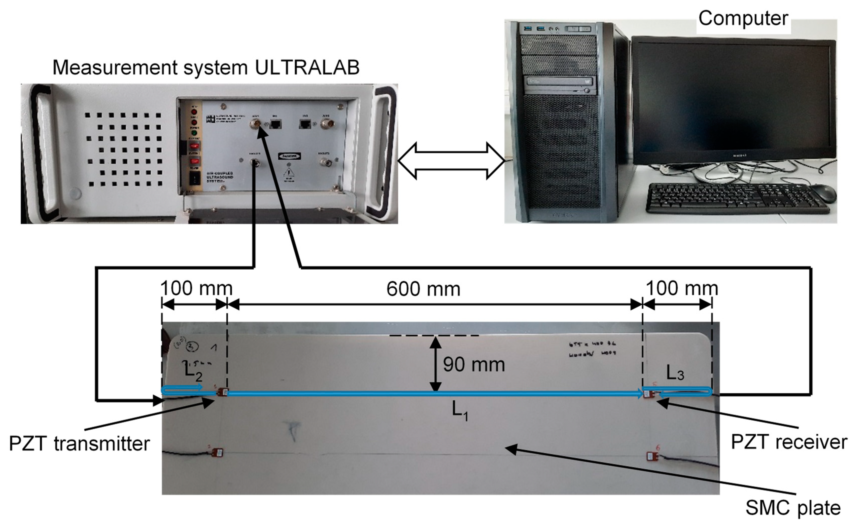
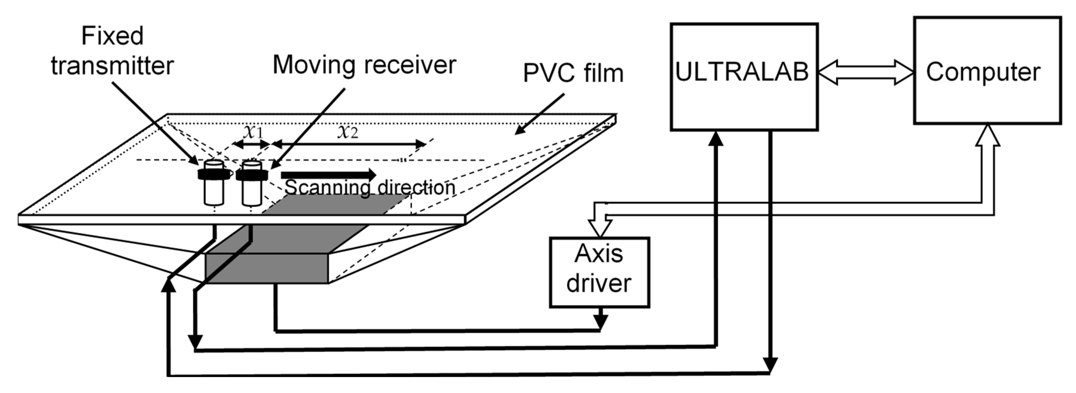
3. Experimental Signal Processing by the Proposed Method

For the qualitative evaluation of the proposed signal processing method, processing of various experimental signals was carried out. In order to demonstrate the advantages of this method, instead of conventional ultrasound signals, Lamb wave (LW) signals were chosen for signal processing. The advantage of these waves is that they propagate in plates over long distances with low amplitude attenuation. However, they are also characterized by a special property dispersion, i.e., depending on the frequency of the signals, their phase and group velocities vary. Therefore, after the signal travels a certain distance, its shape changes without changing the frequency response. In order to evaluate the versatility of the proposed method, several different cases of experimental data processing were selected.

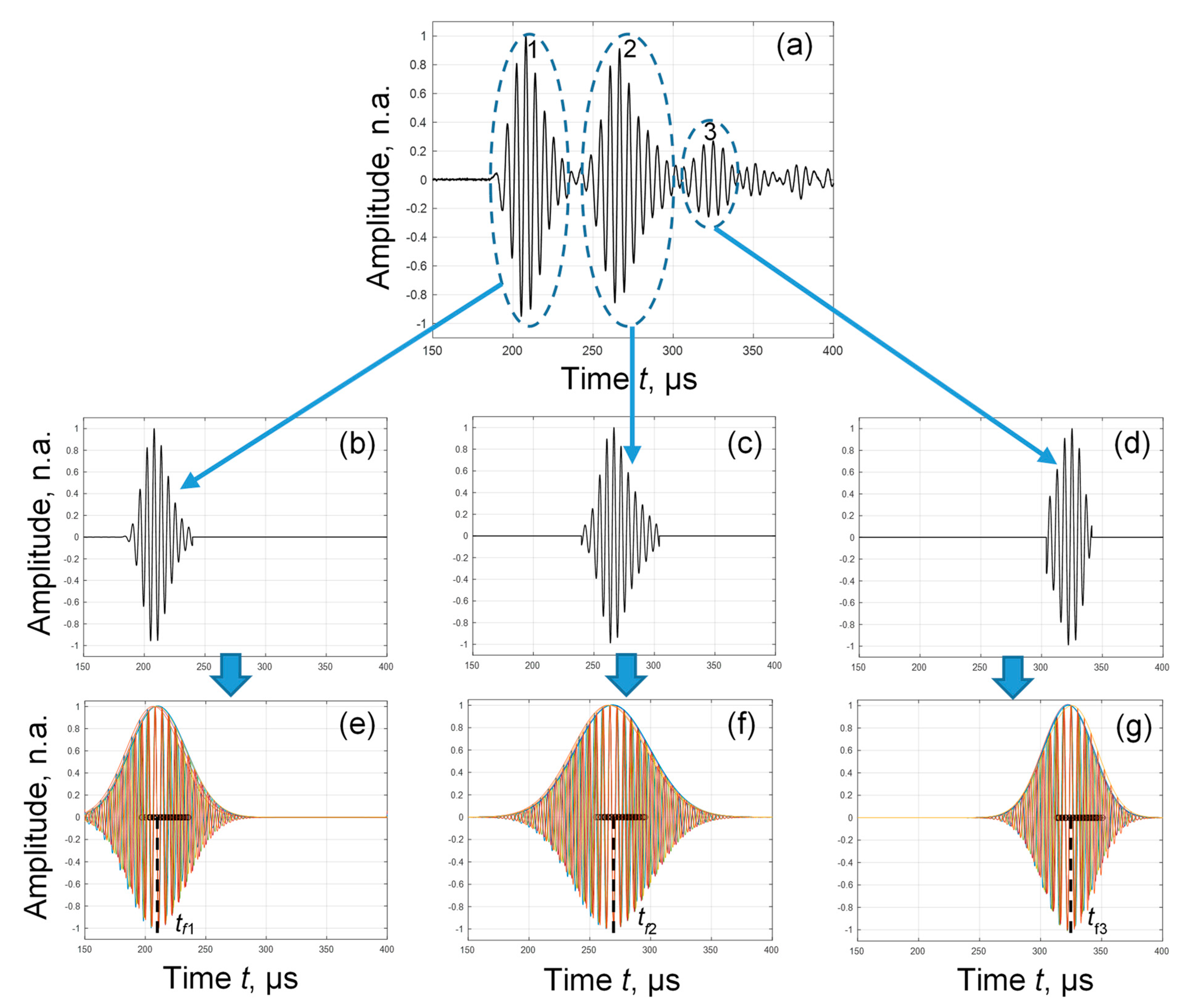
3.1. Estimating the Parameters of the Reflected Signals

The simplest guided wave propagation experiment was performed on a 0.8 × 0.45 m² sheet molding compound (SMC) plate with a thickness of d = 2.3 mm (Figure 4). The ultrasound system “ULTRALAB”, developed at the Ultrasound Research Institute of Kaunas University of Technology, was used in the experiment. In the SMC plate, the S₀ mode of guided waves was generated by PZT contact transducers excited at a resonant frequency f_ex = 180 kHz. The received signal was also recorded by a PZT transducer at a distance of L₁ = 600 mm. A 65 V, 3-period sine signal with a Gaussian envelope was used to excite the transmitter.

The received signal is shown in Figure 5a. In this signal, we can see the directly transmitted signal (direction transmitter–receiver (L₁)) (Figure 5a, (1)), reflections from the edges of the plate (direction transmitter–edge-transmitter–receiver (2L₂ + L₁) and transmitter–receiver–edge-receiver (L₁ + 2L₃)) (Figure 5a, (2)) and double reflection from the edges (direction transmitter–edge-transmitter–receiver–edge-receiver (2L₂ + L₁ + 2L₃)) (Figure 5a, (3)).

The proposed algorithm enables the determination of the propagation times and center frequencies of all these signals. In the given case, we obtained the propagation times of the signals t_f1 = 209.5 µs, t_f2 = 268.0 µs, and t_f3 = 326.5 µs. Meanwhile, the corresponding center frequencies of the signals were f_c1 = 171.1 kHz, f_c2 = 169.5 kHz, and f_c1 = 165.6 kHz. The presented measurement results provide information indicating that the central frequency f_c of the guided wave S₀ modes decreases as they propagate in the plate.

Knowing the propagation time of signals and the distances they travel, it was possible to calculate the propagation velocity of these signals. However, this cannot be done directly for a propagated signal (L1), because the delay time of the exited signal was unknown. The propagation times of two signals (t_f1 and t_f2) that have traveled different distances (L₁ and 2L₂ + L₁) were used to determine the propagation velocity of the signals.

$$c_{S0}={\displaystyle \frac{\left(2L_2+L_1\right)-L_1}{t_{f2}-t_{f1}}}={\displaystyle \frac{2L_2}{t_{f2}-t_{f1}}}=\mathrm{3418.8}\mathrm{m}/\mathrm{s},$$

(20)

This plate was also measured by longitudinal scanning. From the obtained B-scan, the S₀ mode propagation velocity was calculated using the 2D FFT method and was determined to be c_s0 = 3388 m/s. The obtained value differs slightly (0.9%) from the value determined by the proposed method.

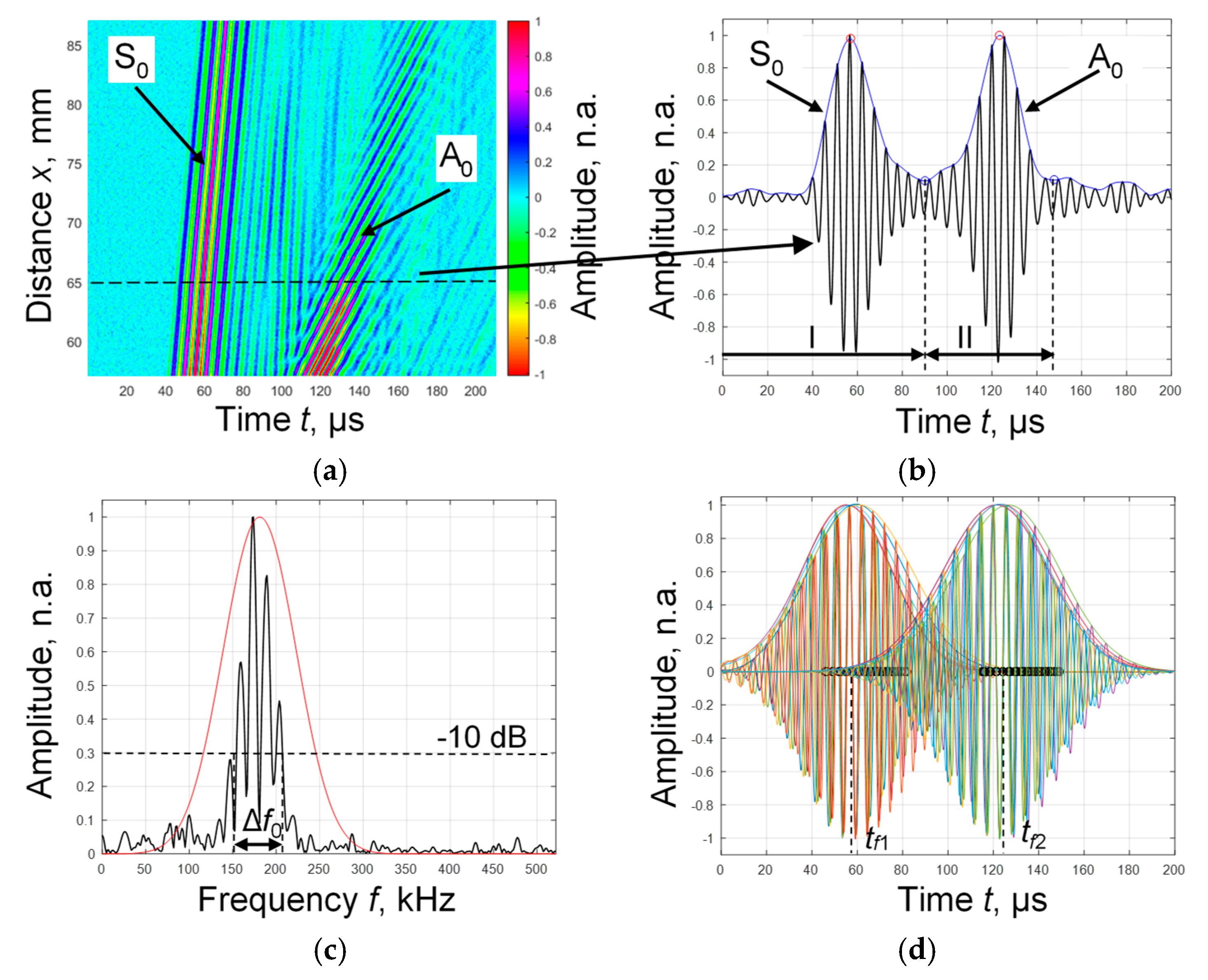
3.2. Separation of the Fundamental Modes

Another case of using the proposed algorithm is the digital processing of signals from experimental studies of d = 200 µm-thick polyvinyl chloride (PVC) film [25]. The film with lateral dimensions 0.21 × 0.297 m² was fixed in a PVC film-mounting bracket (Figure 6).

During the experiments, the S₀ and A₀ Lamb wave modes were excited using contact point transducers with a resonant frequency of 180 kHz. The used transducers were developed at the Ultrasound Research Institute. A 500 V, 3-period sine signal was used to excite the transmitter, and the receiver moved relative to the transmitter over a range of 57 mm to 87 mm. The step of the movement was 0.1 mm.

A B-scan of the distribution of the amplitudes of the received Lamb wave signals, normalized with respect to the maximum value, is shown in Figure 7a.

Figure 7b shows the recorded signal at a distance of 60 mm from the transmitter and the envelope of this signal with the determined maxima and minima. The general frequency response of the analyzed signal is presented in Figure 7c. It also shows the frequency response of the original filter. In the next stage, after using the filter package, the filtered signal packages of individual signals were obtained, and the zero-crossings were determined in them. The obtained results are shown in Figure 7d. In the output of these measurements, it was established that t_f1 = 57.9 µs, t_f2 = 121.4 µs, f_c1 = 181.3 kHz, and f_c2 = 174.9 kHz.

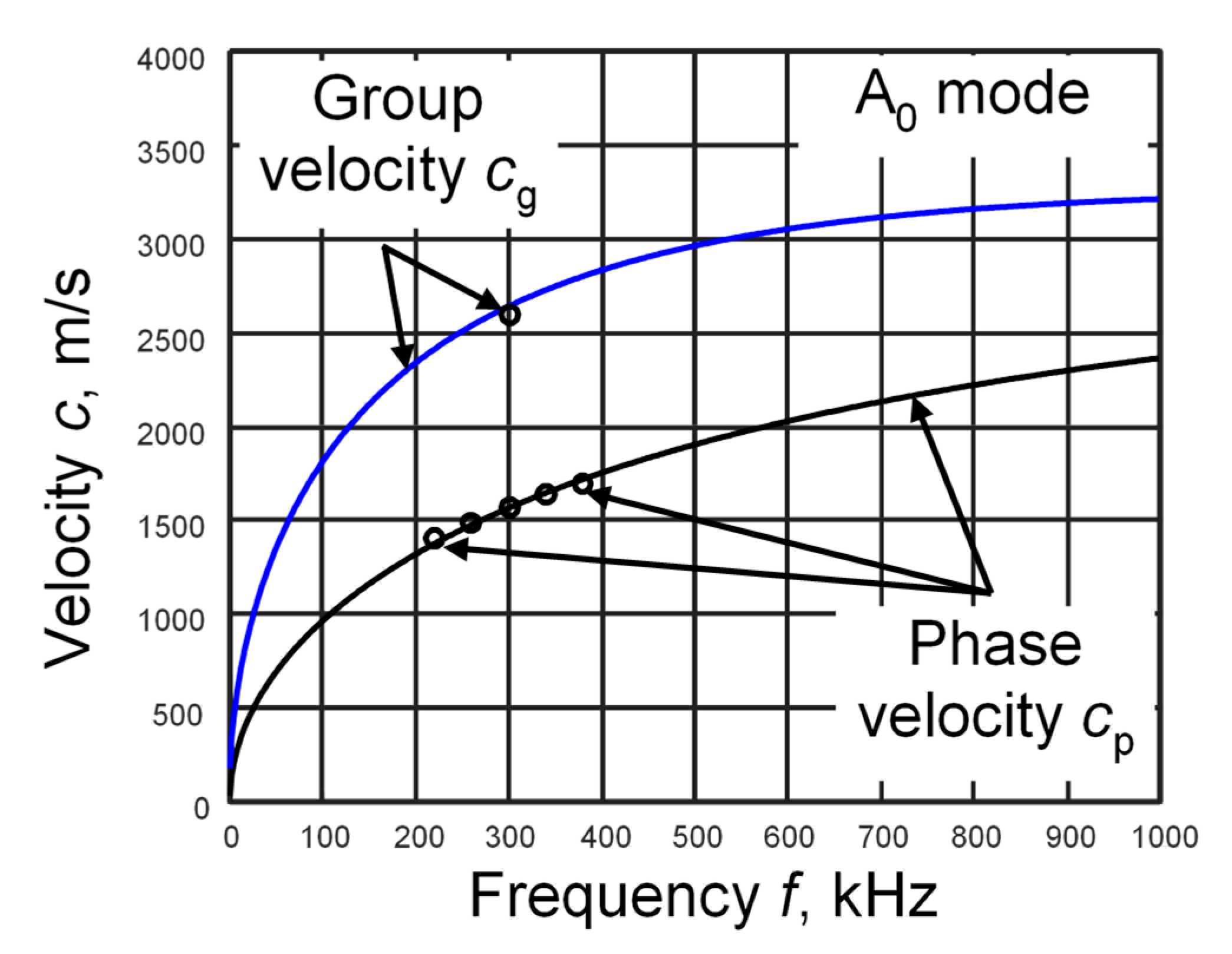
3.3. Phase and Group Velocities Determination

One more case of using the proposed method was to calculate the phase and group propagation velocities of the A₀ mode using the algorithm for determining the propagation time values (ToF) of the ultrasonic signals in the B-scan. The methodology of phase and group velocities estimation is described in detail [23]. We used a typical simulated B-scan image (color coded) (Figure 8a) where the signals propagated in an aluminum plate with a thickness of d = 1 mm, and the excitation frequency of the transmitter was 300 kHz. In the presented B-scan image, together with the simulated signals, the ToF values (line) are plotted (Figure 8a).

As can be seen from the obtained results, the dependence of ToF on distance in narrow ranges was linear (Figure 8b). However, over a wider range, jumps in propagation times are visible. This phenomenon was observed and described in [26]. After using two such jumps, characterized by a set of four points (x_i(1–4), t_i(1–4)) (Figure 8b), it was found that line 1 in the distance between two jumps (x_i2 ÷ x_i3) describes the phase velocity, and line 2 (x_i2 ÷ x_i4) describes the group velocity.

$$c_{\mathrm{p}i}\left(x_{i2}÷x_{i3}\right)={\displaystyle \frac{x_{i3}-x_{i2}}{t_{i3}-t_{i2}}},$$

(21)

$$c_{\mathrm{g}i}\left(x_{i2}÷x_{i4}\right)={\displaystyle \frac{x_{i4}-x_{i2}}{t_{i4}-t_{i2}}}.$$

(22)

Based on the ToF values shown in Figure 8b, the calculated values of phase and group velocities in the narrow range are, respectively, c_p = 1567.5 m/s and c_g = 2594.3 m/s.

Using the ToF calculation methodology and the group and phase velocity estimation method, the segments of the A₀ mode dispersion curve of isotropic materials were calculated [23]. The values of these segments were compared with the theoretical dispersion curves of the A₀ mode, calculated by the one-dimensional SAFE method (Figure 9).

Group and phase velocities calculated by this method differed by no more than 0.7% from values calculated by the SAFE method.

In addition, the phase velocity of the S₀ mode can be calculated using this method. This methodology was described in [27].

4. Discussion and Conclusions

This article proposes a simplified approach to determine the time-of-flight (ToF) of signals based on the use of zero-crossing times of filtered signals to calculate these parameters. Together with the ToF, the center frequency of the signal was also determined. The proposed method was adapted to the processing of experimental signals obtained during various ultrasound investigations. By processing S₀ mode signals propagating in the SMC plate, the propagation velocity of this mode was calculated. Its value was compared with the value obtained by the 2D FFT method. The obtained results differed by 0.9%. Using simulated signals propagating in 1 mm-thick aluminum, the phase and group velocity segments of the A₀ mode were calculated. Their values differed by 0.7% from the theoretically calculated values of the dispersion curves by the SAFE method.

The results obtained during these investigations confirmed the effectiveness of the method and highlighted its advantages in comparison with other methods. Unlike threshold and peak-based methods, uncertainties due to the noise level in the signal are avoided. No threshold for signal capture is required. It is suitable for signals with a reasonably low signal-to-noise ratio. Compared to the correlation method, there is no need to have a reference signal. As an additional parameter, the center frequency of the signal was set. In the proposed method, all signal processing procedures can take place in an automated mode, depending on the signal’s frequency response, by selecting the bandwidths of the filters. This enables the use of the method in automated measurements.

However, this method has some limitations in terms of the signal processing algorithm. The overlap of multiple signals limits the application of the method, as the absence of envelopes for individual signals does not provide the ability to separate those signals. In the case of a low signal-to-noise ratio, the frequency characteristic of the signal can no longer be distinguished automatically. This can be done manually, and further processing of the signals was not affected in this case.

However, the discussed shortcomings do not diminish the possibilities of applying this signal processing method for processing both ultrasonic and acoustic signals.

References

1. Xu, B.; Yu, L.; Giurgiutiu, V. Advanced methods for time-of-flight estimation with application to lamb wave structural health monitoring. In Proceedings of the 7th International Workshop on Structural Health Monitoring, Stanford, CA, USA, 9–11 September 2009. [Google Scholar]
2. Raya, R.; Frizera, A.; Ceres, R.; Calderón, L.; Rocon, E. Design and evaluation of a fast model-based algorithm for ultrasonic range measurements. Sens. Actuators A Phys. 2008, 148, 335–341. [Google Scholar] [CrossRef]
3. Chen, Q.; Li, W.; Wu, J. Realization of a multipath ultrasonic gas flowmeter based on transit-time technique. Ultrasonics 2014, 54, 285–290. [Google Scholar] [CrossRef] [PubMed]
4. Kim, Y.H.; Song, S.J.; Lee, J.K. Technique for measurements of elastic wave velocities and thickness of solid plate from access on only one side. Jpn. J. Appl. Phys. 2005, 44, 5240–5243. [Google Scholar] [CrossRef]
5. Jenot, F.; Ouaftouh, M.; Duquennoy, M. Corrosion thickness gauging in plates using Lamb wave group velocity measurements. Meas. Sci. Technol. 2001, 12, 1287–1293. [Google Scholar] [CrossRef]
6. Hoseini, M.R.; Wang, X.; Zuo, M.J. Estimating ultrasonic time of flight using envelope and quasi maximum likelihood method for damage detection and assessment. Measurement 2012, 45, 2072–2080. [Google Scholar] [CrossRef]
7. Hull, D.R.; Kautz, H.E.; Vary, A. Measurement of ultrasonic velocity using phase-slope and cross-correlation method. Mater. Eval. 1985, 43, 1455–1460. [Google Scholar]
8. Svilainis, L. Review of high resolution time of flight estimation techniques for ultrasonic signals. In Proceedings of the 52nd Annual Conference of the British Institute of Non-Destructive Testing, Telford, UK, 10–12 September 2013. [Google Scholar]
9. Khyam, M.O.; Ge, S.S.; Li, X.D.; Pickering, M.R. Highly Accurate Time-of-Flight Measurement Technique Based on Phase-Correlation for Ultrasonic Ranging. IEEE Sens. J. 2017, 17, 434–443. [Google Scholar] [CrossRef]
10. Jia, L.; Xue, B.; Chen, S.; Wu, H.; Yang, X.; Zhai, J.; Zeng, Z. A High-Resolution Ultrasonic Ranging System Using Laser Sensing and a Cross-Correlation Method. Appl. Sci. 2019, 9, 1483. [Google Scholar] [CrossRef]
11. Hirata, S.; Kurosawa, M.K.; Katagiri, T. Real-time ultrasonic distance measurements for autonomous mobile robots using cross correlation by single-bit signal processing. In Proceedings of the IEEE International Conference on Robotics and Automation, Kobe, Japan, 12–17 May 2009; pp. 3601–3606. [Google Scholar] [CrossRef]
12. Cai, C.; Regtien, P.P.L. Accurate digital time-of-flight measurement using self-interference. IEEE Trans. Instrum. Meas. 1993, 42, 990–994. [Google Scholar] [CrossRef]
13. Wang, X.F.; Tang, Z.A. A novel method for digital ultrasonic time-of-flight measurement. Rev. Sci. Instrum. 2010, 81, 105112. [Google Scholar] [CrossRef] [PubMed]
14. Jackson, J.C.; Summan, R.; Dobie, G.I.; Whiteley, S.M.; Pierce, S.G.; Hayward, G. Time-of-flight measurement techniques for airborne ultrasonic ranging. IEEE Trans. Ultrason. Ferroelectr. Freq. Control 2013, 60, 343–355. [Google Scholar] [CrossRef] [PubMed]
15. Liu, W.; Li, D.; Xie, W. A novel time-of-flight difference determination method for ultrasonic thickness measurement with ultrasonic echo onset point detection. Appl. Acoust. 2025, 233, 110605. [Google Scholar] [CrossRef]
16. Lu, Z.; Ma, F.; Yang, C.; Chang, M. A novel method for Estimating Time of Flight of ultrasonic echoes through short-time Fourier transforms. Ultrasonics 2020, 103, 106104. [Google Scholar] [CrossRef] [PubMed]
17. Pomponi, E.; Vinogradov, A.; Danyuk, A. Wavelet based approach to signal activity detection and phase picking: Application to acoustic emission. Signal Process. 2015, 115, 110–119. [Google Scholar] [CrossRef]
18. Zhou, H.; Li, P.; Wu, L.; Gao, Q. A wavelet analysis-based matching pursuit algorithm for an accurate ultrasonic TOFD measurement. Insight 2020, 62, 662–668. [Google Scholar] [CrossRef]
19. Laddada, S.; Lemlikchi, S.; Guendouzi, F.; Si-Chaib, M.O.; Djelouah, H. Ultrasonic time of flight estimation using Wavelet transforms. In Proceedings of the 7th African Conference on Non Destructive Testing (ACNDT) & the 5th International Conference on NDT and Materials Industry and Alloys (IC-WNDT-MI), Oran, Algeria, 26–28 November 2016. [Google Scholar]
20. Sturtevant, B.; Velisavljevic, N.; Sinha, D.; Kono, Y.; Pantea, C. A broadband wavelet implementation for rapid ultrasound pulse-echo time-of-flight measurements. Rev. Sci. Instrum. 2020, 91, 075115. [Google Scholar] [CrossRef] [PubMed]
21. da Silva, J.H.B.; de Oliveira, L.D.; Villanueva, J.M.M. Application of Wavelet Transform for Ultrasonic Time of Flight Estimation. In Proceedings of the 6th International Symposium on Instrumentation Systems, Circuits and Transducers (INSCIT), Porto Alegre, Brazil, 22–26 August 2022; pp. 1–6. [Google Scholar] [CrossRef]
22. Cheeke, J.D.N. Fundamentals and Applications of Ultrasonic Waves; CRC Press: Boca Raton, FL, USA, 2012; pp. 1–504. [Google Scholar] [CrossRef]
23. Tumšys, O. Experimental method for simultaneous determination of the Lamb wave A0 modes group and phase velocities. Materials 2022, 15, 2976. [Google Scholar] [CrossRef] [PubMed]
24. MATLAB. User’s Manual. Available online: https://www.mathworks.com/help/matlab/index.html (accessed on 20 September 2024).
25. Kažys, R.; Tumšys, O. Simultaneous measurement of thickness and elastic properties of thin plastic films by means of ultrasonic guided waves. Sensors 2021, 21, 6779. [Google Scholar] [CrossRef] [PubMed]
26. Mažeika, L.; Draudvilienė, L.; Žukauskas, E. Influence of the dispersion on measurement of phase and group velocities of Lamb waves. Ultragarsas (Ultrasound) 2009, 64, 18–21. Available online: https://www.ultragarsas.ktu.lt/index.php/USnd/article/view/17122 (accessed on 20 September 2024).
27. Tumšys, O.; Mažeika, L. Determining the Elastic Constants of Isotropic Materials by Measuring the Phase Velocities of the A0 and S0 Modes of Lamb Waves. Sensors 2023, 23, 6678. [Google Scholar] [CrossRef] [PubMed]
Figure 1. The block diagram of the proposed algorithm for the digital signal processing of ultrasonic signals with noise.
Applsci 15 05721 g001
Figure 2. The original signal and the signals filtered by a five-filter package.
Applsci 15 05721 g002
Figure 3. 300 kHz original signal (a) and the same signal with white Gaussian noise (signal-to-noise ratio SNR = 20 dB) (b).
Applsci 15 05721 g003
Figure 4. The structural scheme of GW S0 mode signal generation and recording in an SMC plate.
Applsci 15 05721 g004
Figure 5. (a) Received GW signal on SMC plate. (bd) Individual extracted signals. (eg) Determination of propagation times of individual signals.
Applsci 15 05721 g005
Figure 6. The structural scheme of the Lamb wave signal generation and recording in thin PVC film.
Applsci 15 05721 g006
Figure 7. (a) The B-scan of the measured amplitudes of the Lamb wave signals in the PVC film of the thickness d = 200 µm. (b) The signal recorded at a distance of 60 mm from the transmitter and the envelope of this signal with the determined maxima and minima. (c) Signal and filter frequency response. (d) Signals filtered by a filter package, and zero-crossings fixed in these signals.
Applsci 15 05721 g007
Figure 8. (a) Calculated values of the ToF (line) using simulated Lamb wave A0 mode signals (color coded). (b) Values of the ToF in the narrow range.
Applsci 15 05721 g008
Figure 9. Segments of phase and group velocities calculated using the proposed methodology (dots) and dispersion curves calculated using the SAFE method (lines).
Applsci 15 05721 g009