Applying Methods of Exploratory Data Analysis and Methods of Modeling the Unemployment Rate in Spatial Terms in Poland

Abstract

The level of unemployment in a region can be a good illustration of its socio-economic development. The choice of the data modeling method, both in terms of spatial and time-spatial approaches depends on the results of exploratory data analysis. The aim of the research is to investigate which methods of GIS spatial analysis can be used for the cartographic presentation of the variability of the unemployment rate in Poland, broken down into provinces (voivodeships) and districts in terms of time and space. This goal will be achieved by performing an exploratory analysis of data on the unemployment rate in Poland for the period 2004–2022 in order to select the methods of cartographic presentation and transfer in spatial and time-spatial terms, along with selected cartographic methods in the GIS of the level of unemployment in Poland. This study, excluding data analysis based on statistical tests, focuses on examining the distribution of unemployment rates in Poland by districts and provinces from 2004 to 2022. This leads to the selection of optimal methods for the visualization and analysis of spatial data. The use of data analysis methods based on statistical tests and the examination of the distribution of data on the unemployment rate in Poland at county (district) and province (voivodeship) level for the period 2004–2022 will be performed in order to validate the results of the research. The selection of optimal methods of visualization and analysis of spatial data is intended to be a model for use in other areas of research.

1. Introduction

The purpose of this article is to model the unemployment rate, which gives a good indication of the level of socio-economic development of regions. A spatial description of unemployment as a description of negative socio-economic phenomena is an important task of spatial econometrics, while modeling economic processes must be characterized by spatial dependencies [1]. The spatial analysis of unemployment rates has been widely studied, utilizing various modeling techniques [2,3,4]. A spatial approach requires the use of exploratory data analysis (EDA) and based on the results of this analysis, selecting the most appropriate visualization methods. This problem has been described in foreign literature [5,6,7,8] and in Polish literature [9,10]. EDA is the basis for making decisions about the choice of space-modeling tools [11]. According to Filiztekin [12], most of the models presented in the literature (see the comprehensive review in [13]) discuss the existence of unemployment disparities, but do not necessarily relate them to geography. Therefore, in Filiztekin’s research, Moran’s I test is calculated to examine the role of location in shaping the distribution of unemployment. The investigation of spatial clustering effects also requires an analysis of the spatial distribution of unemployment rates [14], as well as the application of statistical tests of spatial dependence to assess the non-random distribution of neighboring regions, as emphasized by the authors. Studying regional unemployment rates necessitates demonstrating positive spatial autocorrelation, revealing clusters of geographically adjacent regions with similar unemployment levels through the use of Moran’s I test [15]. Understanding the persistence of regional unemployment requires the consideration of spatial heterogeneity [16]. Regional models that incorporate spatial factors often provide a deeper insight into unemployment trends, particularly in areas affected by labor market transformations [17]. The analysis of spatial patterns in economic activity helps identify factors that influence regional unemployment rates [18]. In practice, Moran’s I tests are applied to both large [19] and small samples [20], and spatial autocorrelation indices provide evidence of spatial interactions between regions, which must be accounted for in the regression analyses and spatial modeling of unemployment rates, for instance, by using Moran’s scatterplots [21,22]. To analyze and visualize spatial patterns, researchers employ Local Indicators of Spatial Association (LISA) statistics [23] and Getis-Ord Gi* statistics [24,25], including their extensions for spatio-temporal analysis [26]. Visualization tools such as choropleth maps and cartograms are used, taking into account the heterogeneity of administrative units, both for regression models and for representing unemployment rates [7,27,28]. Additionally, Kernel Density Estimation (KDE) is used for spatial visualization [29].

In this publication, the type of distribution, characteristics, and statistical data such as the unemployment rate for various locational (spatial) approaches will be examined and determined. For this purpose, an exploratory analysis of data will be used, in GIS software (ArcGIS Pro 3.4), in regards to the unemployment rate measured in provinces, districts, and cities in Poland. Then, following the analysis of statistical test results, appropriate spatial modeling methods will be selected and applied. he aim of the article is to examine the unemployment rate in Poland as statistical data and its spatial analysis at the provincial level for the period 2004–2022, and at the district and city level in 2021 using statistically justified data modeling tools in GIS. The innovativeness of the proposed approach lies in the application of advanced spatial analysis methods for visualizing and modeling unemployment, integrating not only classical statistical indicators but also geostatistical techniques to assess local trends and spatial heterogeneity, thereby enabling more precise decision-making in labor market policy.

The authors posed the following research questions: Do traditional methods of unemployment analysis adequately reflect their spatial structure? Which spatial analysis techniques provide the most accurate representation of unemployment distribution and support decision-making in labor market policies? To what extent does exploratory data analysis (EDA) influence the selection of modeling and visualization methods for unemployment rate analysis?

Traditionally, studies on the unemployment rate focus on identifying the causes and factors influencing its level. In this study, a different approach was adopted, whereby the primary objective of the analysis was to achieve the best possible spatial representation of the phenomenon. To this end, exploratory data analysis (EDA) was used as the foundation for spatial analysis. Additionally, it was examined whether the data exhibited significant spatial dependencies, which was a key step in further modeling.

2. Materials and Methods

The methodological innovation in this study lies in its shift from traditional unemployment rate analyses, which typically focus on identifying causal factors, to an approach prioritizing the spatial representation of the phenomenon. The study employs exploratory data analysis (EDA) as the foundation for spatial analysis, first testing the null hypothesis of randomness to determine whether unemployment exhibits significant spatial patterns. If the results confirm that unemployment is not randomly distributed, the application of spatial modeling techniques is justified instead of simple visualizations of the average unemployment rate based on administrative boundaries. Interpolation methods, particularly Kriging, were used to create a continuous spatial surface from discrete data, optimizing model selection based on approximation errors compared to actual measurements. This innovative approach enhances precision in representing unemployment distribution, offering a more accurate and detailed spatial depiction of the phenomenon.

The unemployment rate data analyzed in this study were obtained from the official statistics provided by the Polish Central Statistical Office (GUS). The data are calculated using the classical method, based on the official Eurostat definition, ensuring consistency and comparability with other European statistical data. According to the official statistics of the Polish Central Statistical Office (GUS) and Eurostat, the unemployment rate is defined as the ratio of the number of unemployed individuals actively seeking work to the number of economically active individuals. This definition is widely accepted in economic research and ensures comparability with international studies. The dataset covers the period 2004–2022 and is publicly available in the Local Data Bank (https://bdl.stat.gov.pl/BDL/start, 20 January 2025) and the Geostatistical Portal (https://geo.stat.gov.pl/, 20 January 2025), as well as in the annual Statistical Yearbooks published by GUS. This ensures the reliability and transparency of the input data used for spatial analyses presented in this paper. According to Bal-Domańska, this is the most commonly used measure of unemployment, defined as the ratio of the number of people who are unemployed but actively seeking work to the number of economically active individuals [30]. In the literature, numerous studies focus on modeling unemployment changes in Poland [31], which can be classified into those utilizing spatial analyses and those employing GIS for visualizing the results of econometric research. All of these studies address the spatial variation of unemployment levels in Poland [32,33], with some specifically dedicated to the application of spatial analyses [34]. Spatial models extend classical econometric models by incorporating so-called spatial effects: spatial dependence and spatial heterogeneity [35,36]. Although these studies most commonly address the spatial aspect in a modeling context [37] or focus on correlations with potential factors [22,38].

The authors formulated the following research hypotheses:

H1. 

Traditional methods of unemployment analysis, based on administrative divisions, may distort the actual spatial structure of this phenomenon, justifying the need for spatial analysis methods.

H2. 

Exploratory data analysis (EDA) facilitates the optimal selection of modeling and visualization methods for unemployment rate analysis, improving result interpretation accuracy and enhancing its application in labor market policy.

H3. 

The application of spatial analysis techniques allows for a more precise identification of unemployment distribution patterns, enabling better-targeted policy interventions and resource allocation in labor market planning.

The data modeling process applied in this study follows a universal scheme (Figure 1).

The results of EDA determine the further selection of visualization methods and spatial analyses. This approach ensures that the applied tools are statistically justified and aligned with the nature of the data. Unfortunately, this methodological rigor is not always maintained, and the validation parameters are often omitted, which significantly reduces the credibility and reliability of such data. The first stage is to perform a spatial autocorrelation analysis (using Global Moran’s I). Next, the nearest neighbor analysis is applied to evaluate spatial clustering tendencies. Data distribution analysis, using charts, histograms, and QQ plots, helps assess whether the data meet normality assumptions. Finally, outlier detection is performed using Thiessen polygons and Voronoi diagrams. The visualization and modeling method is selected based on the results of these analyses. If the null hypothesis of random data distribution is confirmed, the recommended visualizations include choropleth maps, diagrams, graduated symbols, and proportional symbols. However, if the null hypothesis is rejected, spatial interpolation techniques (both geostatistical and deterministic) can be applied without methodological concerns. Additionally, model optimization is performed using the parametric estimation quality assessment method (MPQE), and advanced spatial analyses such as the hot spot analysis and Kernel Density Maps are recommended to identify significant spatial patterns.

A spatial dependency analysis was conducted in ArcGIS Pro, and appropriate methods for visualizing the unemployment rate were selected based on the results of EDA, which comprises a set of statistical techniques used to characterize observations exhibiting spatial relationships.

In the first step, the EDA will be performed using a spatial autocorrelation analysis (Global Moran’s I). This is based on the binary matrix of weights, and the significance of Moran’s I statistic is carried out by means of a test in which the following hypotheses are verified [39]:

H0. 

Spatial autocorrelation does not occur.

H1. 

There is a spatial autocorrelation.

In the second step of the EDA, the average test of the nearest neighbor will be performed. If the index is less than 1, the pattern shows grouping; if the index is greater than 1, the tendency is towards dispersion or competition [40,41]. In the third step of the EDA, the type of data distribution instruments of the histogram and QQ diagram will be examined. Understanding data distribution is an important step in the data-mining process [42]. For comparison, you can add a normal distribution overlay to the histogram [43]. Normal QQ plots, like histograms, make it possible to study the effect of logarithmic transformations and square roots on the distribution of data while comparing them with the normal distribution [44]. In the fourth step of the EDA, outliers will be tested using Thiessen polygons. Each Thiessen polygon contains only one point entry function. Each location in a Thiessen polygon is closer to its associated point than to any other input function of the point. The resulting Voronoi diagrams are used to determine the outliers. A global outlier is a measured sampling point that has a very high or very low value relative to all values in the dataset. A local outlier is a measured sample point that has a value within the normal range for the entire dataset, but if you look at the surrounding points, it is unusually high or low [45].

The next stage of work will be the selection of spatial statistics tools for visualization. Statistics are divided into descriptive and inferred statistics (statistical tests). In the case of descriptive statistics, classification depends more on the choices and methods of the analyst, rather than the results of statistical tests. In statistical tests, on the other hand, the analysis is more likely to result in clusters whose size, shape or distribution cannot be influenced by the analyst because they are formed automatically according to the algorithm assigned to the analysis technique. If the null hypothesis with a random distribution of data is confirmed, then cartograms, diagrams, graduated, and proportional symbols will be made, while if the null hypothesis is rejected, data interpolations and the optimization of models will be performed using the parametric estimation quality assessment method. In addition, hot spot analyses and density maps using the Kernel method will be performed.

A cartogram represents a phenomenon within the boundaries of a given territorial unit by color, shade or hatching. Depending on the situation and the intention of the analyst, this fact can make the cartogram overly general, which can be seen as a disadvantage. Another disadvantage of the cartogram is the freedom to choose a scale that can change the appearance of a given phenomenon [46]. Pie charts are often used to represent the overall value of a phenomenon (expressed in the area of a circle) and the percentage of its components, giving the reader a quick idea of the proportional distribution of data [47]. In the next step, maps will be performed using geostatistical methods. In this work, maps will be carried out using the Kriging method. Each measurement z(x) is the implementation of the function of the random variable Z(x) (where x- means the location in the area), i.e., if the measurement was performed several times at point x, the measurement results will be different. However, in any pair of points xn and xn + h, the random variables Z(xn) and Z(xn + h) are bound by a certain correlation relationship resulting from the spatial continuity of the studied phenomenon [48]. Data modeling is carried out using the semivariogram analysis. The course of the semivariogram function indicates at what rate the interaction of variables decreases with the increasing distance [49]. In terms of spatial statistics, measurement values are treated as a regionalized variable (also called spatial or localized), which is defined as a continuous coordinate function of space. The values of this regionalized variable are known only at the place of measurement, and there are a few of them compared to the studied space. In order to be able to perform a statistical interpretation on a regionalized variable, certain restrictions are imposed on it. In particular, the hypothesis of a weak stationary is assumed, which means that the expected value of the variable does not depend on the place of measurement and its covariance is only a function of the distance between the measurement points. In practice, because the hypothesis of a weak stationary in relation to real parameters is very strict, a much milder limitation is applied, which assumes that poor stationary is not from the regionalized variable itself, but from its increments. Of significant importance here is the variance of increments, which defines the basic characteristic function of geostatistics, known as the semivariogram [50]. In addition, when modeling a space using a semivariogram, the condition of positive definiteness must be met, or more precisely, the semivariance function must meet this condition. This mathematical condition is met by the function families used in ArcGIS PRO (Nugget effect model, Spherical model, Gaussian model, Power model, Exponential model, and Linear model). In these function models, the Kriging function equations can be solved. The indicators that were considered when comparing the results of spatial analyses are the statistical characteristics of the interpolation error:

(a)

Mean prediction error (MSE);

(b)

Root mean square prediction error (RMSE);

(c)

Average standard error (ASE);

(d)

Mean standardized prediction error (MSE);

(e)

Root mean square standardized prediction error (RMSSE).

During the modeling, the scheme of the optimal selection of approximated functions was used [51]: If the values of the interpolation parameters and the semivariogram model were chosen correctly, meaning that the results of the spatial analysis are satisfactory, then:

(a)

MSE = 0;

(b)

RMSE = smallest value;

(c)

ASE should have a value close to RMSE. If ASE is greater than RMSE, then this indicates that the variability in the dataset has been overestimated; conversely, this means underestimating volatility;

(d)

MSE = 0;

(e)

RMSSE = 1.

• Formula 1.

If this error exceeds 1, then the variability in the dataset has been overestimated; if it is less than 1, we are dealing with an underestimation of volatility.

To verify the optimal method, the proprietary method of parameter assessment of the quality of estimation (MPQE) was used, which is based on an optimization algorithm determined both during cross validation and subset validation [52]:

• C1, C2,… Cm—assessment of the quality of estimation;
• D1, D2… Dn—weight;
• a1a2… an—parameter a;
• b1b2… bn—parameter b;
• n1n2… nn—parameter n.

Δ₁a₁ + Δ₂b₁ +… + Δ_nn_n = C₁
Δ₂₁a₂ + Δ₂₂b₂ +… + Δ_2nn_n = C₂
Δ_n1a_n + Δ_n2b_n+ … + Δ_mn_m = C_n

(1)

• Formula 2.

This geostatistical method, whose parameter Cn is close to or equal to 0, is the optimal method:

Cn ≤ 0 = max

(2)

For the purposes of this study, the algorithm was adapted by supplementing the method with an additional three parameters from cross validation and three parameters from subset validation. This algorithm was adapted to the scheme of optimal selection of the modeling method when approximating functions:

• a₁a₂… a_n—parameter a—average error for 100% of data;
• b₁b₂… b_n—parameter b—square root of the average error for 100% of data;
• c₁c₂… c_n—parameter c—average error for 100% of data;
• d₁d₂… d_n—parameter d—average standard error for 100% of data;
• e₁e₂… e_n—parameter e—average standardized error for 100% of data;
• f₁f₂… f_n—parameter f—square root of the mean standardized error for 100% of data;
• g₁g₂… g_n—parameter g—average error for 90% of data;
• h₁h₂… h_n—parameter h—square root of the mean error for 90% of data;
• i₁i₂… i_n—parameter i—average error for 90% of data;
• J₁J₂… j_n—parameter j—average standard error for 90% of data;
• k₁k₂… k_n—parameter k—average standardized error for 90% of data;
• l₁l₂… l_n—parameter l—square root of the mean standardized error for 90% of data;
• Parameter weights: Δb and Δh are 30%, and the other parameters are 5% each.

In the next step, a hot spot (Gi* Getisa–Orda) will be developed. This tool identifies statistically significant spatial clusters with high values (hot spots) and low values (cold spots). It creates an output feature class with a z-score, a p-value, and a confidence interval field for each object in the input class. Z-scores and p-values are measures of statistical significance that tell you whether to reject the null hypothesis. As a result, they indicate whether the observed spatial grouping of high or low values is more pronounced than would be expected in a random distribution of the same values. The z-score and p-value fields do not reflect any type of FDR (False Discovery Rate) correction [53]. Another spatial analysis will be density analysis, the Kernel density tool, using non-parametric estimation using the Epanechnikov kernel [54].

• Formula 3.

This calculates the size per unit area based on point or polyline features using the Kernel function to fit a smoothly conical surface to each point or polyline. The barrier can be used to change the influence of functions when calculating the density of the nucleus [55].

$$\begin{gathered} {\mathit{f}}_{\mathit{\lambda }}\left(\mathit{x}\right)={\displaystyle \frac{\mathbf{1}}{\mathit{n}\mathit{\lambda }}}\mathsf{\Sigma }{\mathit{k}}_{\mathbf{0}}\left({\displaystyle \frac{\mathit{x}-{\mathit{x}}_{\mathit{i}}}{\mathit{\lambda }}}\right) \\ {k}_0\left(t\right)=\left\{\begin{array}{c}0.75\left(1-t^2\right)\\ 0 \end{array}\right. \end{gathered}$$

(3)

where

• k₀—quadratic kernel function;
• L—smoothing parameter;
• for t ≤ 1 in other cases.

3. Results

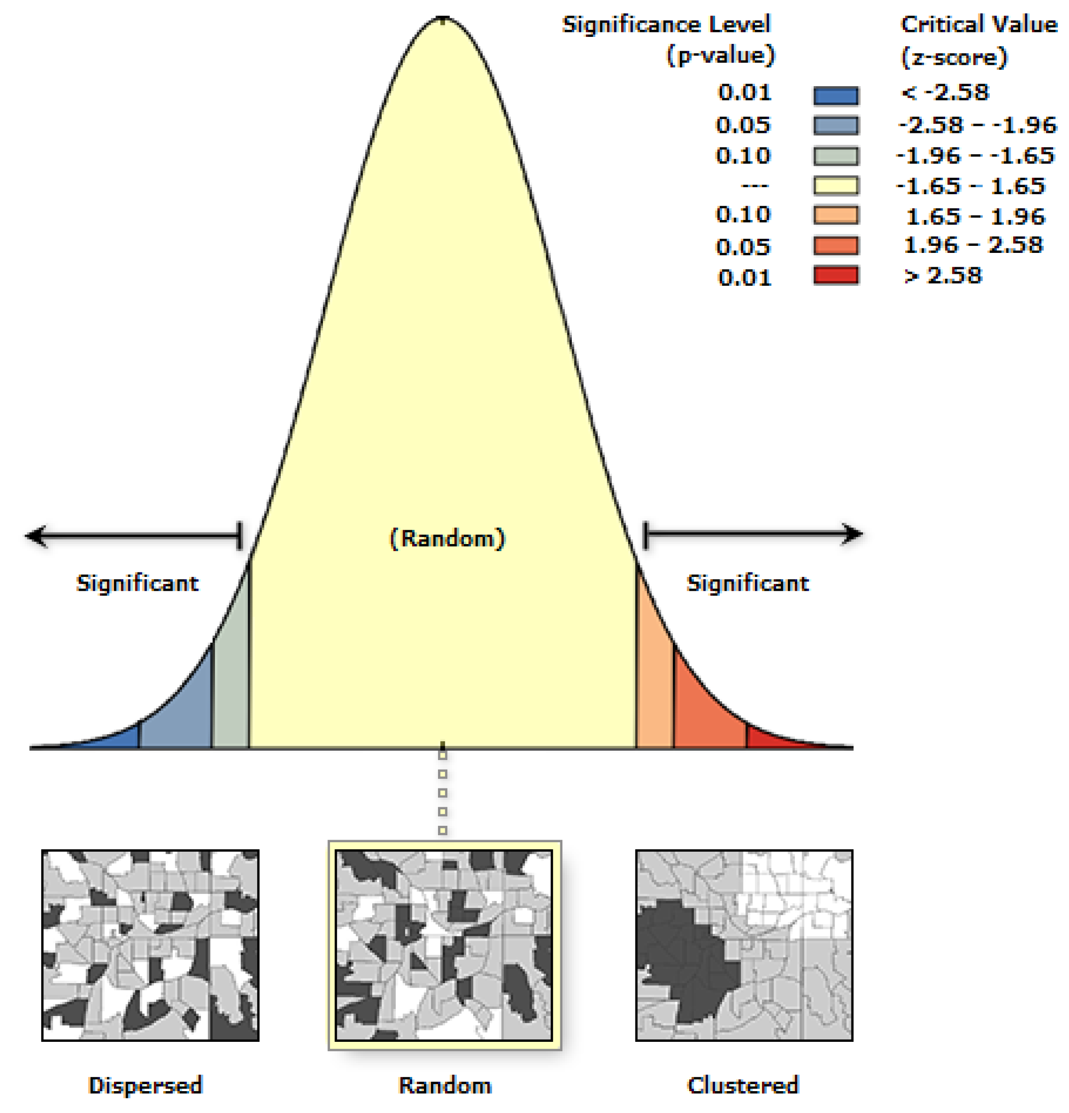
The research process begins, as shown in Figure 2, with exploratory data analysis (EDA), which serves as the foundation for selecting further spatial analysis and visualization methods. Figure 2 shows the results of Moran’s I test for data on the unemployment rate broken down by voivodship.

Data for the period 2004–2022 were verified. In each case, the result was the same, namely, confirming the truth of hypothesis 0. From this, it follows that there is no autocorrelation of data (random distribution).

Figure 3 shows the results of Moran’s I test for data on the unemployment rate broken down by district.

For data on the unemployment rate in counties, the null hypothesis was also confirmed, which means that the data are distributed randomly. Also, in this case, no data autocorrelation was found, which limits the possibilities of data visualization using inferred spatial statistics.

Figure 4 shows the results of Moran’s I test for urban unemployment rate data.

Based on Figure 4, we conclude that the data are clustered, and therefore the null hypothesis about the randomness of their distribution should be rejected.

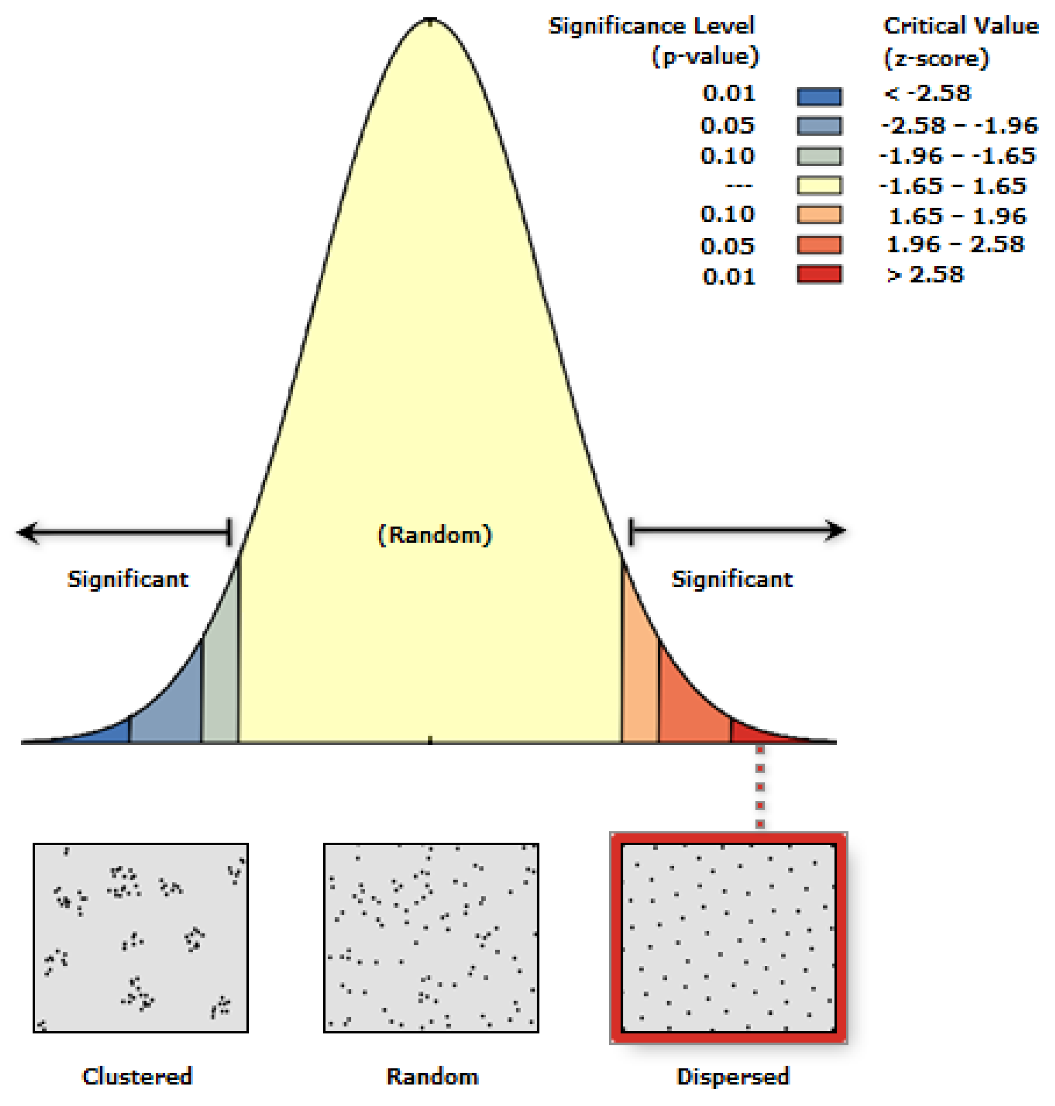
In order to examine whether the distribution of data on the unemployment rate is random or not, a test was carried out for the point data of the nearest average neighbor for the city of Poland. Figure 5 shows the results of the nearest neighbor average test.

Based on Figure 5, we conclude that the null hypothesis is rejected. A result of 4.601594 was obtained, from which it was confirmed that there is a probability of less than 1% that the scattered samples can be the result of a random variable.

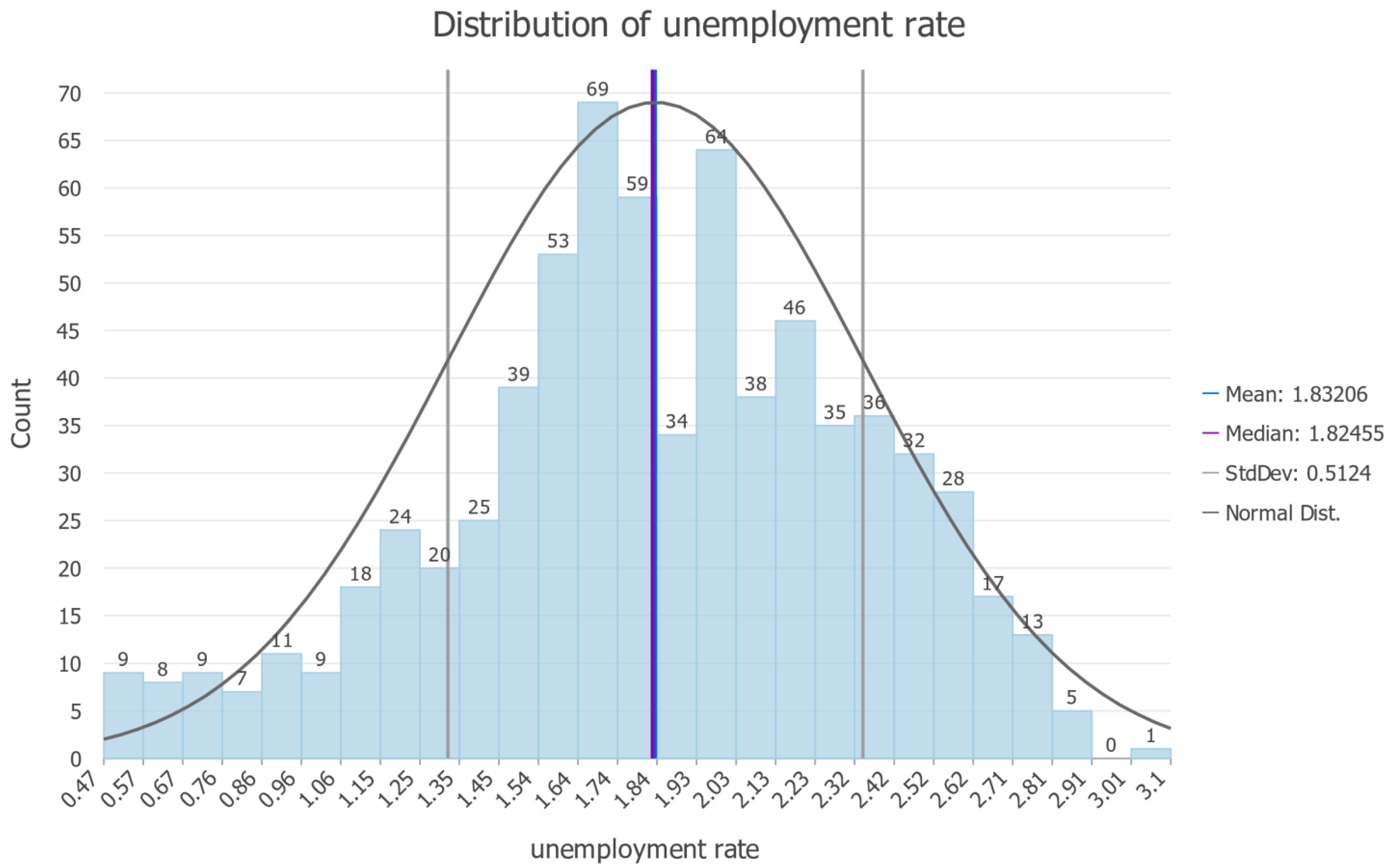
In the next stage, the distribution of data was examined. Figure 6 presents the histogram for data on the unemployment rate in cities.

During the study, it was established that parameters close to the normal system are achieved when a logarithmic transformation is used. This is an important indication during geostatistical modeling that should be considered in the process of space modeling. In addition, if the subset validation method is used for the map validation process, it should be examined whether the distribution of data will change significantly after taking the data into the test set. The histogram for data without a test set is shown in Figure 7.

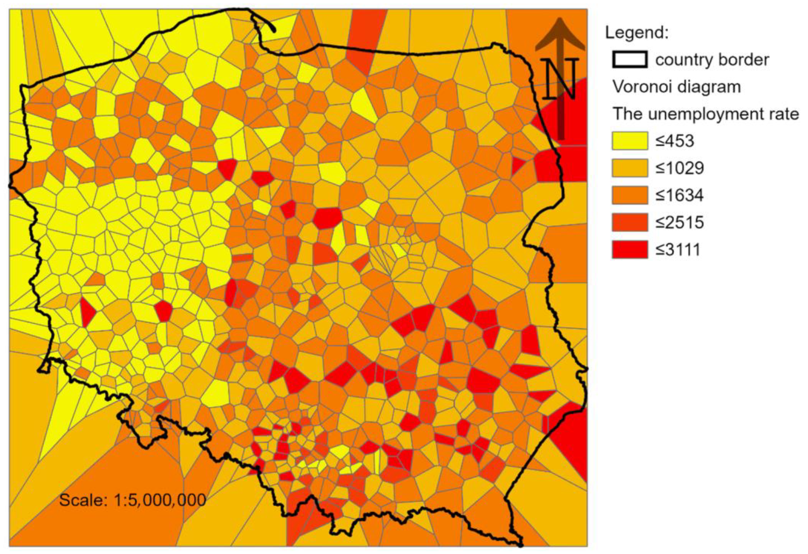
Based on Figure 7, it can be concluded that performing a logarithmic transformation has brought the data distribution closer to a normal distribution. Therefore, during modeling, the analyst should take this information into account and, particularly when using the Kriging method, apply the logarithmic transformation in the geostatistical wizard. The next step of the EDA is to examine the outliers based on Thiessen polygons and the analysis of the Voronoi diagram, as shown in Figure 8.

Based on Figure 8, we conclude that there are reflective values of the percentage rate. These data should be carefully analyzed, as there is a higher probability of measurement error. However, for a data type such as the percentage rate, the possibility of a spike in distribution is likely; therefore, none of the data will be removed in the main study.

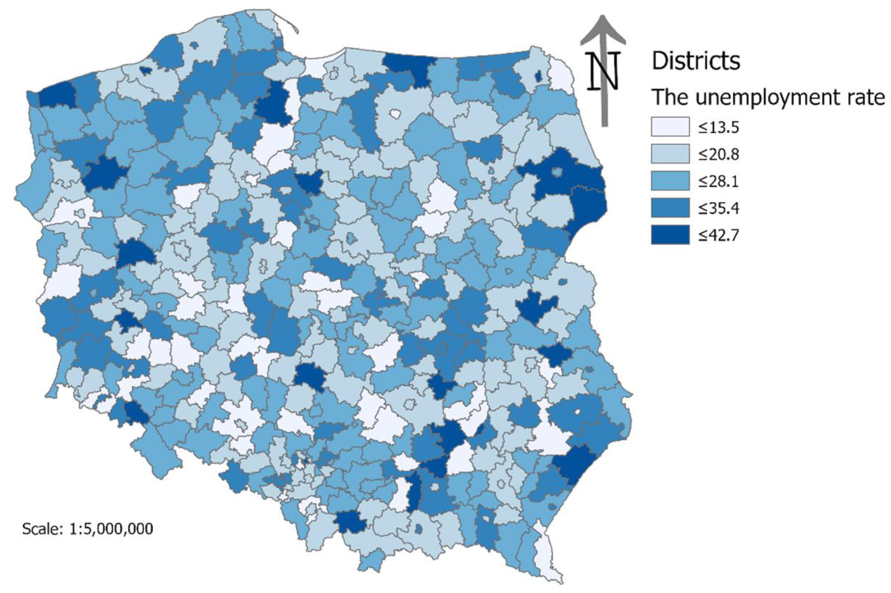
Based on the results of research in EDA, data on the percentage rate for the area of districts were presented in the form of a diagram in Figure 9.

Figure 9 confirms the conclusions drawn from the EDA that assigning statistical characteristics to large areas and drawing strong conclusions on this basis flattens the perspective and the reliability of results. In addition, data on the percentage rate in provinces and districts do not have the form of a normal distribution, and classification using standard deviation should not be used during the classification, which makes it even more difficult to make correct inferences. Figure 10 shows the result of the hot spot for the unemployment rate.

A hot spot analysis allows the clusters of the unemployment rate to be interpreted using Getis and Ord statistics. This enables the differentiation of the strength of the significance of the highlighted clusters of events, depending on the strength of local autocorrelation [54]. Based on Figure 10, we conclude that the percentage rate brings together several cities into clusters with the same values. Therefore, the creation of a continuous surface of the phenomenon is justified. Although it should not be related to the cadastral units of the area, it is possible to impose their boundaries onto maps made using the techniques of inferred statistics.

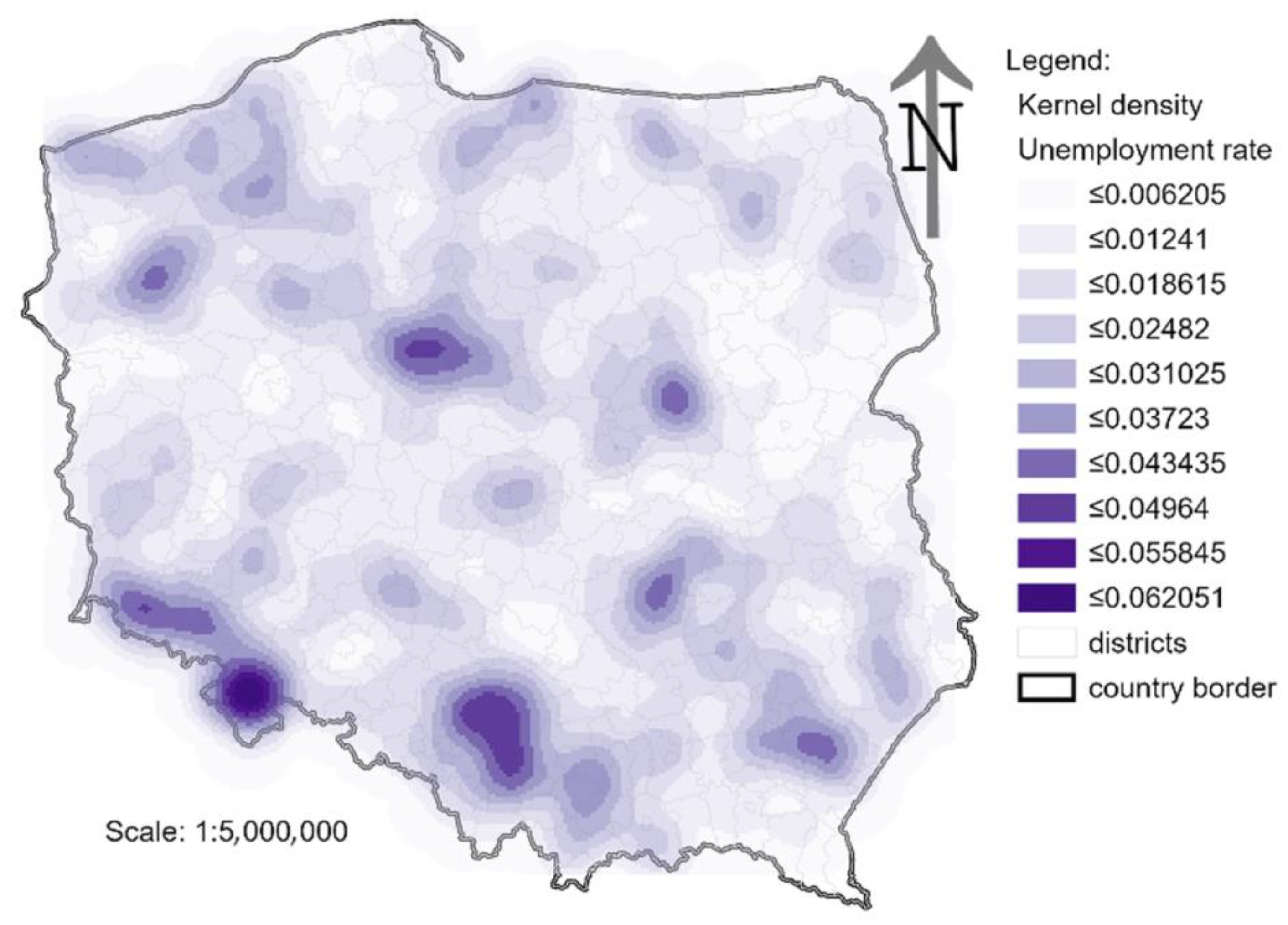
Figure 11 shows the results of the Kernel [56] analysis of the nuclear density unemployment rate. Although this method is traditionally used for large point datasets, recent literature highlights its increasing application in socio-economic studies with a limited number of observations [57,58]. However, in this study, the Kernel Density Estimation (KDE) method was applied as one of the techniques for visualizing the spatial distribution of unemployment rates. Its application aimed to capture spatial continuity and smooth transitions between unemployment rates in neighboring cities. In this context, KDE also enables the identification of local concentrations and areas with increased unemployment risk, making it a valuable tool in spatial analyses of socio-economic phenomena. The resulting map in Figure 11 is in the form of a continuous value of the unemployment rate and the hot spots visible on it; in this way, it focuses on values. Figure 11 also shows the boundaries of districts to confirm the above-described defects of cartograms and diagram charts describing the value of the unemployment rate. In addition, it can be determined whether the problem of high unemployment is homogeneous within administrative boundaries of districts, or whether it occurs in localized parts. It is also possible to say where there is no problem because the unemployment rate is low.

Figure 12 shows maps made by geostatistical methods, which are developed based on the percentage rate values of cities recorded in the Geodatabase. In the process of modeling percentage rate data, the principles of process optimization were applied. The presented results are therefore the optimal version of the map for a given method.

Based on Figure 12, it is difficult to indicate which of the maps is optimal. A parametric estimation quality method was used to validate the maps. The results of the validation process are presented in

Table 1. Cross validation result.

Method	ME	RMSE	MSE	RMSSE	ASE	MPQE
KO	0.009	3.154	0.002	0.787	3.893	2.3615
KS	0.266	3.243	0.054	0.874	3.64	2.4292
EBK	0.045	3.325	0.055	0.943	3.394	2.4387
KU	0.026	3.489	0.132	18.154	0.191	3.9437

Source: Own author’s draft based on data from the GIS data modeling validator.

,

Table 2. Subset validation result.

Method	ME	RMSE	MSE	RMSSE	ASE	MPQE
EBK	0.011	2.443	0.003	0.975	2.483	1.4737
KO	0.065	2.464	0.003	0.9	3.129	1.8881
KS	0.124	2.467	0.022	0.932	2.582	1.8462
KU	0.49	2.92	2.92	1.704	0.167	2.2801

Source: Own author’s draft based on data from the GIS data modeling validator.

and

Table 3. Validation result by the parametric assessment of estimation quality.

Method	MPQE CW	MPQE SW	MPQE
EBK	2.4387	1.4737	1.9562
KO	2.3615	1.8462	2.10385
KS	2.4292	2.2801	2.35465
KU	3.9437	2.2801	3.1119

Source: Own author’s draft based on data from the GIS data modeling validator.

.

Based on the data contained in Table 1, Table 2 and Table 3, we conclude that the optimal geostatistical method for mapping the unemployment rate is the Empirical Bayesian Kriging (EBK) method presented in Figure 13. Studies have shown that these differences are statistically significant.

Figure 13 shows the division of provincial unemployment rate distribution without displaying the voivodeship borders. Also, in this case, we can assign provinces that differ in the unemployment rate within the administrative unit. The map shows the spatial diversity of the examined feature and allows for the analysis of places with a high unemployment rate. In addition, it is noticeable that administrative boundaries do not affect changes in value, and the spatial locations of cold and warm places are areas that are not dependent on the administrative unit. The phenomenon of low and high percentage rates generates areas that can be compared to irregularly shaped buffers.

4. Discussion and Conclusions

The innovativeness of the proposed approach lies in the application of spatial analysis methods to the unemployment rate calculated by classical methods at the city level, instead of relying solely on traditional averages computed for administrative units. The conventional approach, widely used in spatial studies, often leads to data oversimplification, resulting in artificially homogeneous representations of socio-economic conditions. However, the analyses conducted in this study clearly demonstrate that administrative areas are, in fact, spatially heterogeneous, and this local variability should be properly considered both in scientific research and in policy-making processes.

The proposed methodology, combining classical unemployment rate calculation with spatial analysis techniques, allows this spatial heterogeneity to be captured. Furthermore, the data modeling scheme described in the article, based on exploratory data analysis (EDA), ensures that the selection of visualization and modeling methods is statistically justified. This enables spatial interpolation, allowing for the estimation of unemployment rates in towns and cities where direct measurements are unavailable. Importantly, statistical tests confirmed the reliability of these estimations, since the spatial distribution of the unemployment rate exhibits clear patterns rather than randomness. An additional benefit of this approach is the identification of local anomalies and spatial outliers, which can be of particular relevance for labor market policies and regional development strategies.

The conducted analyses confirmed that spatial analyses applied to unemployment rate data at the city level provide a much more detailed and reliable picture of spatial disparities than traditional approaches based on aggregated administrative units. Moran’s I test showed a statistically significant spatial autocorrelation, justifying the use of spatial statistics. In contrast, when using polygon data for provinces or districts, descriptive statistics may be more appropriate. This highlights a key methodological contribution of this study—demonstrating that spatial unemployment patterns within administrative units are often masked when only averaged values per unit are considered.

Moreover, the removal of artificial administrative boundaries in the visualization process allows for more accurate spatial targeting of anti-unemployment policies. This refined approach could help allocate financial support more precisely, directing funds not to entire administrative units, but to the specific cities and subregions where interventions are most urgently needed. This practical application further highlights the relevance of integrating spatial statistics and classical economic indicators in labor market research.

The conducted analyses confirmed hypothesis 1, demonstrating that traditional methods of unemployment analysis, based on the aggregation of administrative data, can distort the actual representation of this phenomenon. Hypothesis 2 was also confirmed, whereby exploratory data analysis (EDA) enabled the optimal selection of modeling and visualization methods, revealing spatial unemployment patterns that were not detectable through traditional statistical analyses. Furthermore, the results validated hypothesis 3, indicating that the integration of GIS-based spatial analysis methods with classical economic indicators allows for a more precise identification of areas requiring intervention, emphasizing the crucial role of spatial analysis in modeling socio-economic phenomena.

The presented approach to spatial unemployment analysis can be applied in a wide range of socio-economic studies, including labor market monitoring, modeling the impact of transportation accessibility on employment, assessing the effectiveness of activation policies, and optimizing the allocation of support funds in regions with the highest unemployment risk. Additionally, the proposed methodology enhances the adaptability of labor market analyses by allowing for dynamic updates as new data become available, ensuring that policy responses can be more timely and data-driven. By integrating spatial interpolation with exploratory data analysis, this approach also provides a robust framework for detecting emerging labor market trends and forecasting potential shifts in unemployment distribution. Furthermore, the combination of classical economic indicators with spatial modeling opens new possibilities for comparative studies across different countries and regions, facilitating cross-border labor market assessments. The flexibility of this method makes it suitable for analyzing not only unemployment, but also other socio-economic phenomena, such as income disparities, workforce migration, and regional economic resilience, providing a comprehensive tool for decision-makers and researchers alike.