


Water Quality Monitoring: A Water Quality Dataset from an On-Site Study in Macao


Abstract
1. Introduction
- Real-time and cost-effective monitoring—By using low-cost sensors and a modular Raspberry Pi-based architecture, the system enables continuous data collection at significantly lower costs than commercial systems [4].
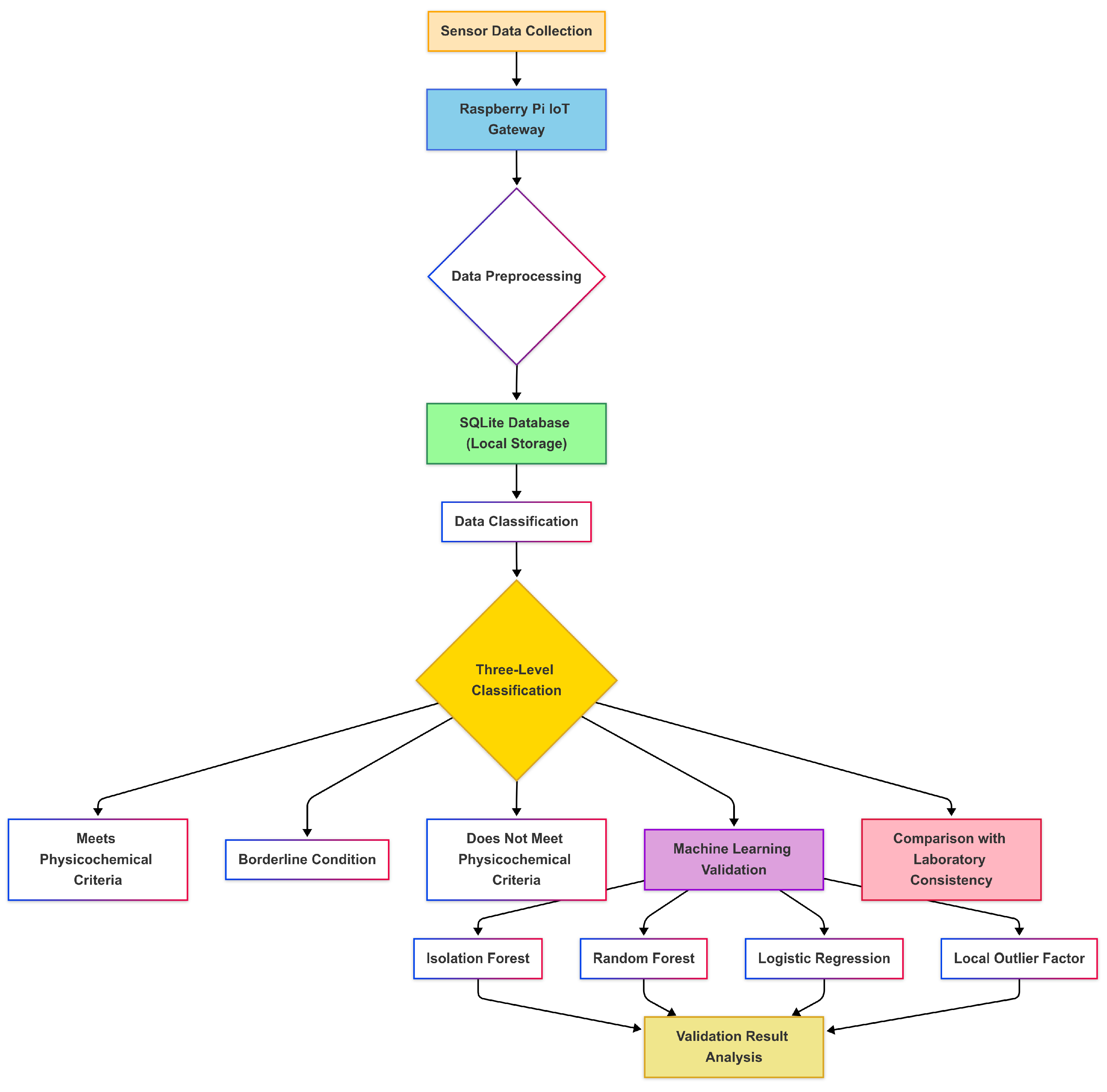
- Comprehensive anomaly detection—A boundary-condition-based triple-classification rule categorizes water quality into normal, borderline, and abnormal states, allowing for early warning and adaptive responses.
- Compliance with international standards—Our system meets 60% of the WHO and EPA physicochemical water quality monitoring criteria, making it a robust alternative for urban water management.
- Macao water quality dataset—We have established a high-quality water quality dataset for Macao, which provides a database for future water management in Macao.
2. System Design
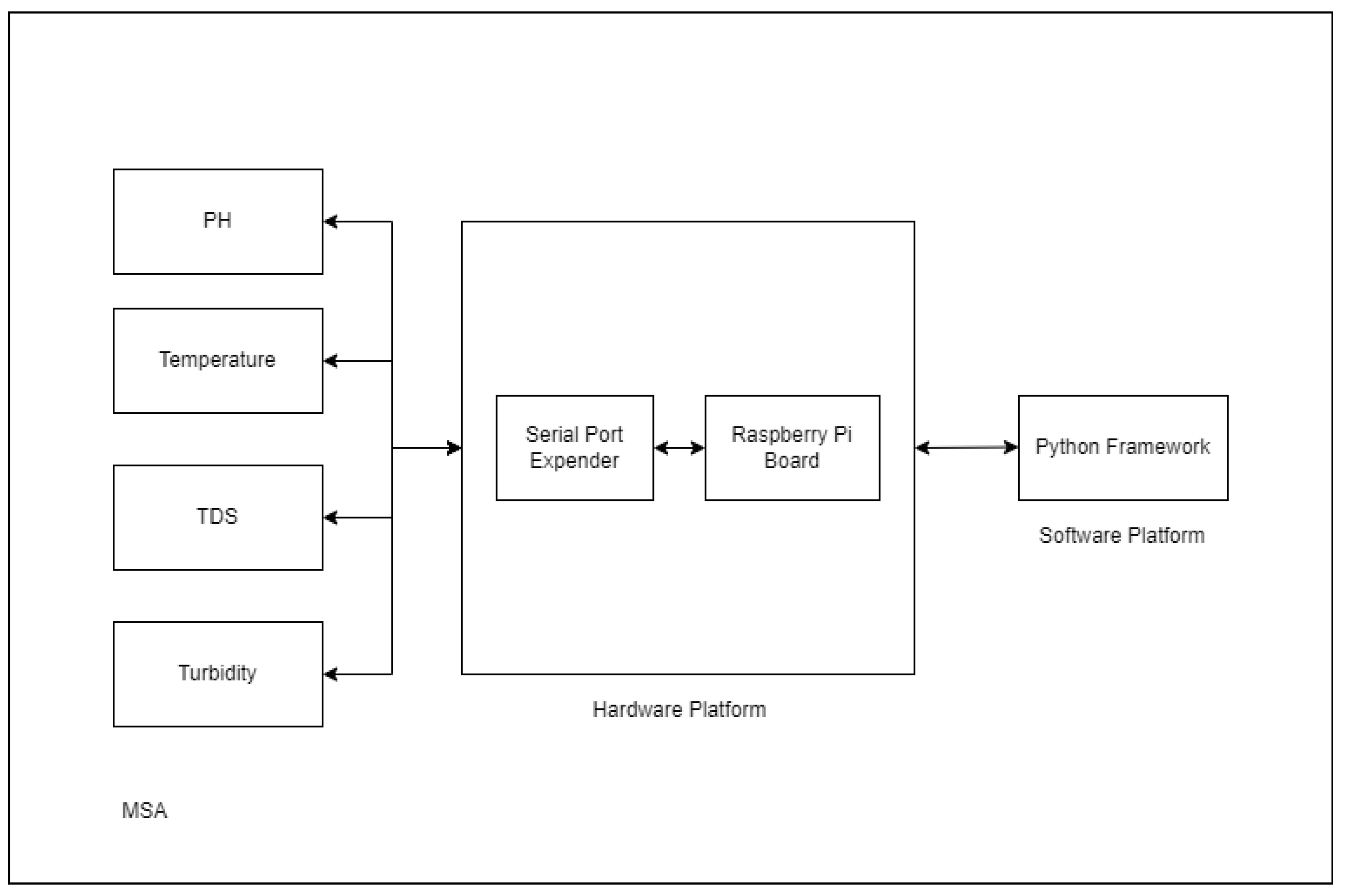
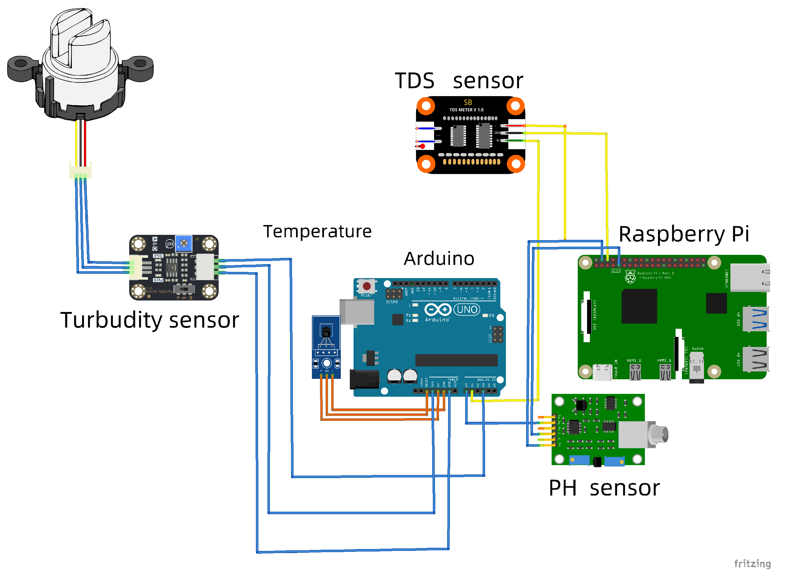
2.1. Hardware Components
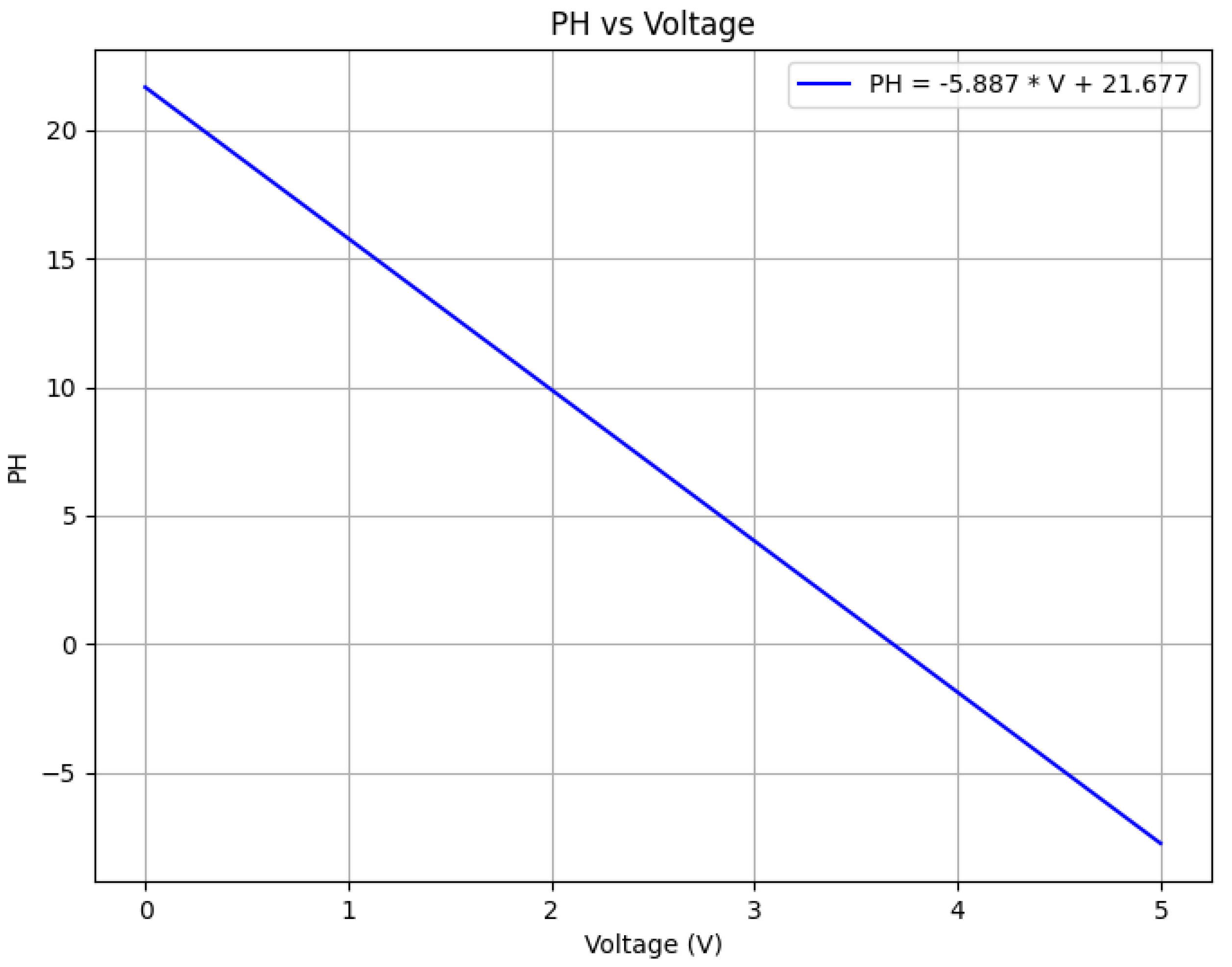
2.1.1. Ph Sensor
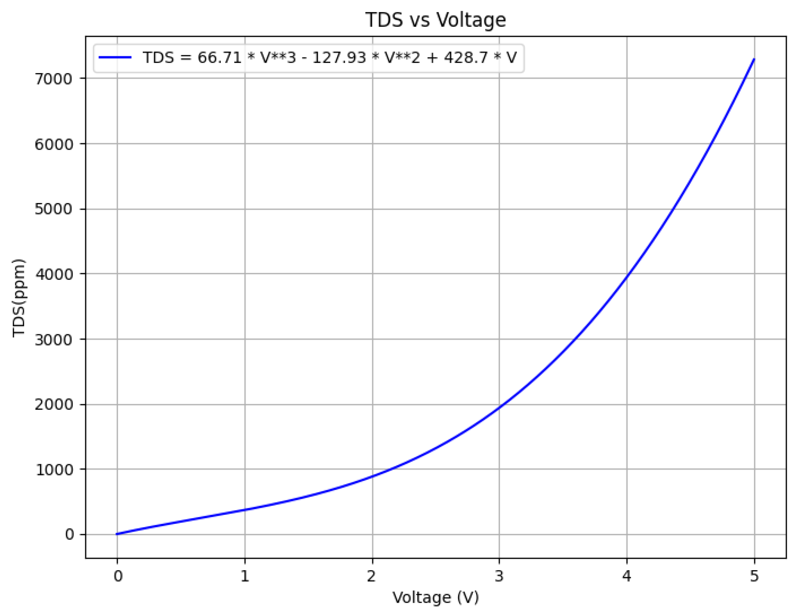
2.1.2. TDS Sensor
- V: Sensor output voltage (in volts, V);
- TDS: Total dissolved solid concentration (in ppm).
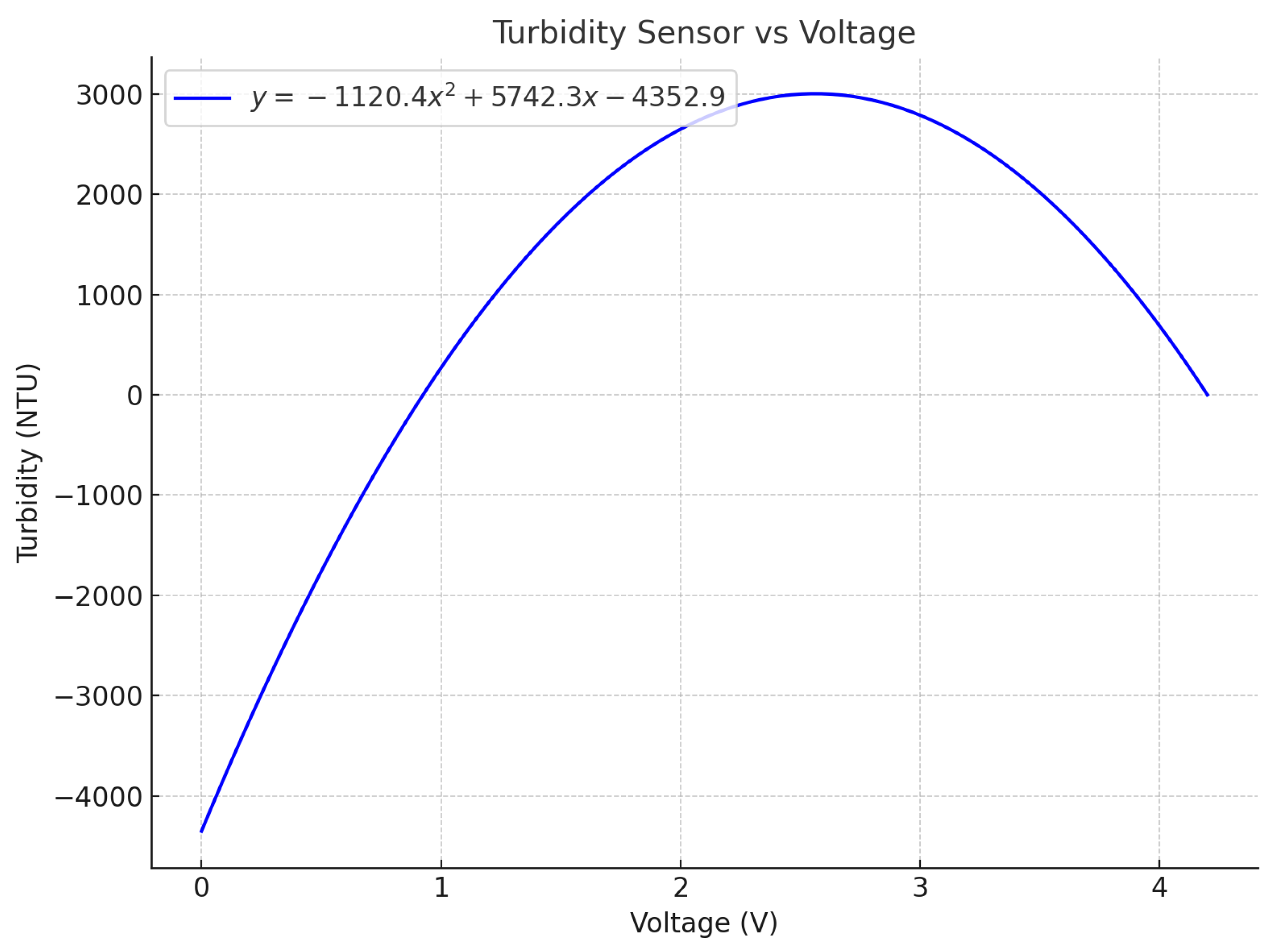
2.1.3. Turbidity Sensor
2.1.4. Temperature Sensor
3. Data Acquisition Methods
3.1. Sampling Location and Duration
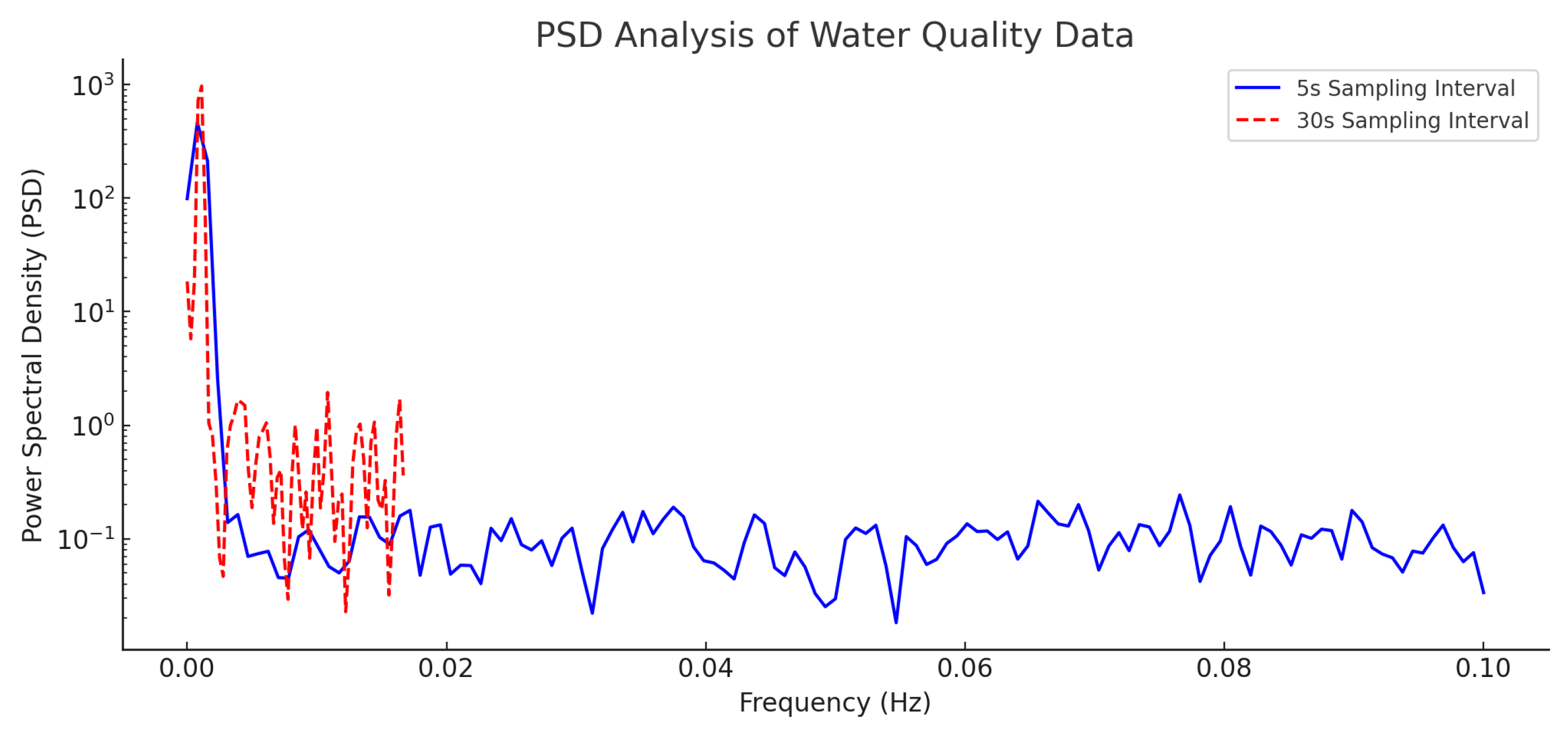
3.1.1. Selection of Sampling Interval
3.1.2. Sampling Point Installation
- Kitchen sinks: Reflecting water used for drinking and cooking.
- Bathroom sinks: Monitoring water used for personal hygiene.
- Toilets: Assessing the quality of water used for flushing [21].
- Utility sinks: Providing insights into water use in dormitory common areas.
3.2. Sensor Calibration
3.2.1. pH Sensor Calibration
3.2.2. TDS Sensor Calibration
3.2.3. DS18B20 Temperature Sensor Calibration
3.2.4. Turbidity Sensor Calibration
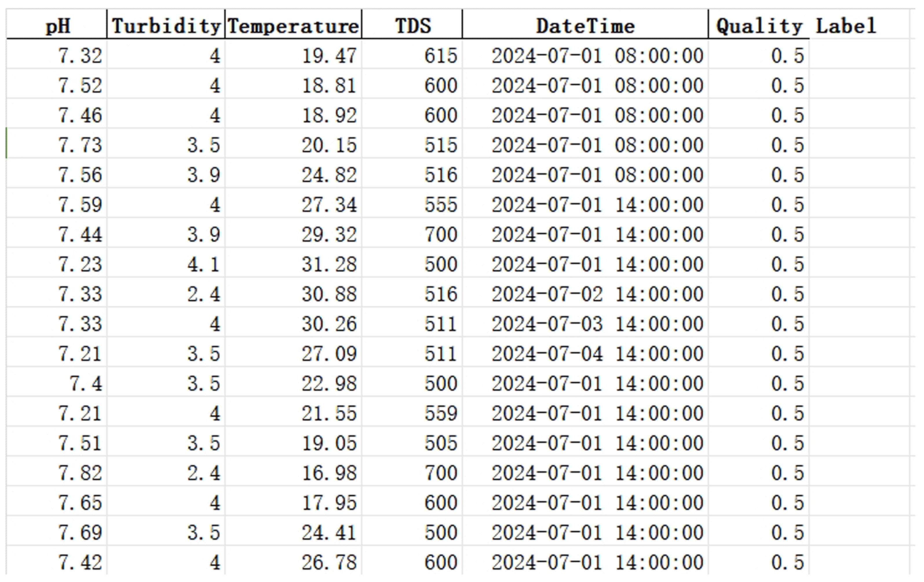
4. Data Description
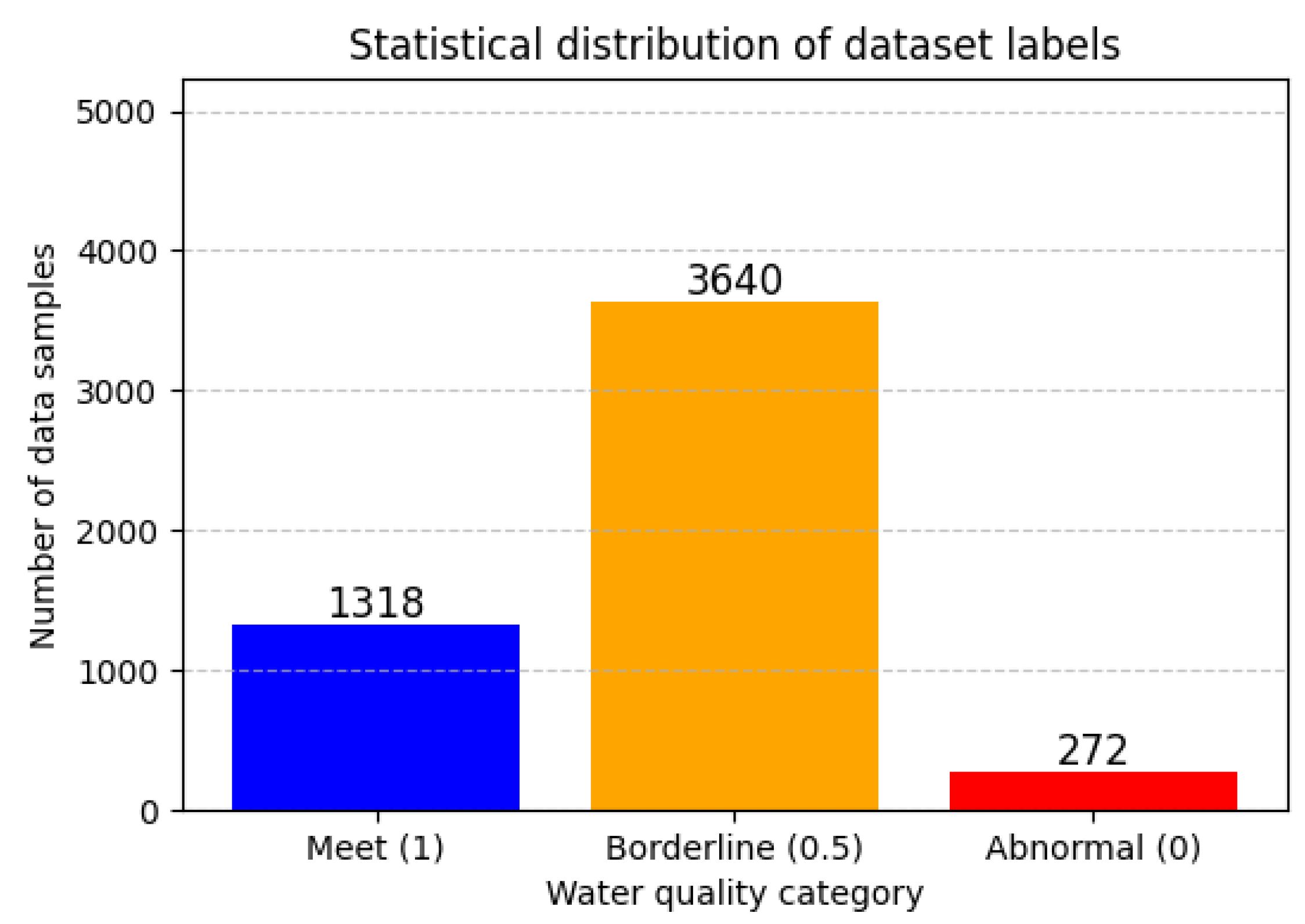
Data Labeling
- Meets Physicochemical Criteria (0.5): 25% of the dataset.
- Borderline Condition (1): 69% of the dataset.
- Does Not Meet Physicochemical Criteria (0): 6% of the dataset.
5. Data Validation
5.1. Data Validation: Comparison with Laboratory Data
5.1.1. Methodology and Data Sources
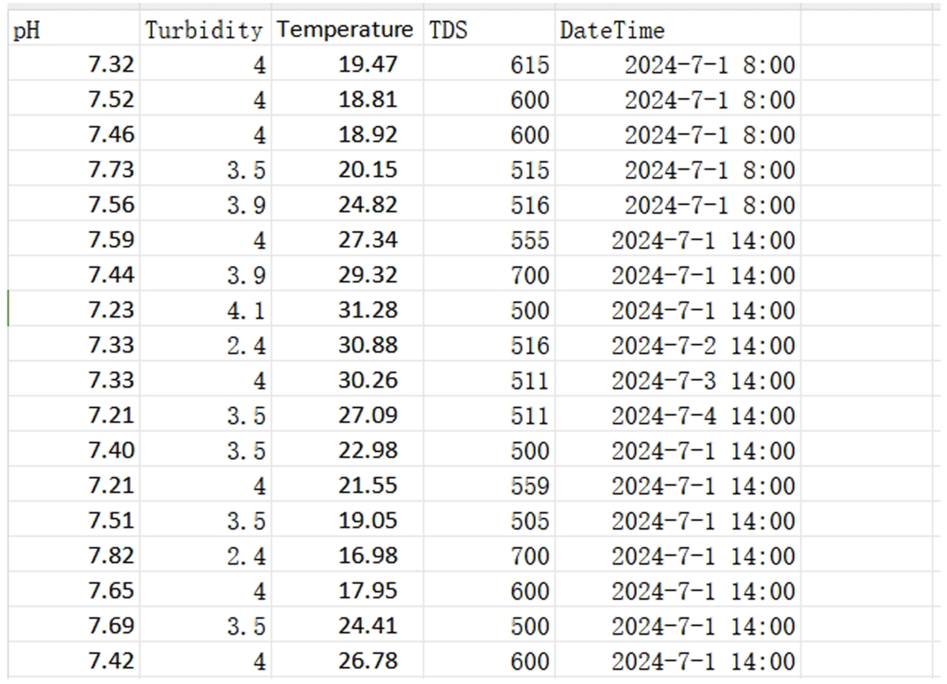
- Experimental data (system measurements): Collected using the Raspberry Pi-based multi-sensor platform, measuring pH, total dissolved solids (TDSs), and turbidity at regular time intervals.
- Reference data (laboratory measurements): Obtained from the Macao Municipal Laboratory website and the Macao Statistics and Census Service’s environmental statistics reports.
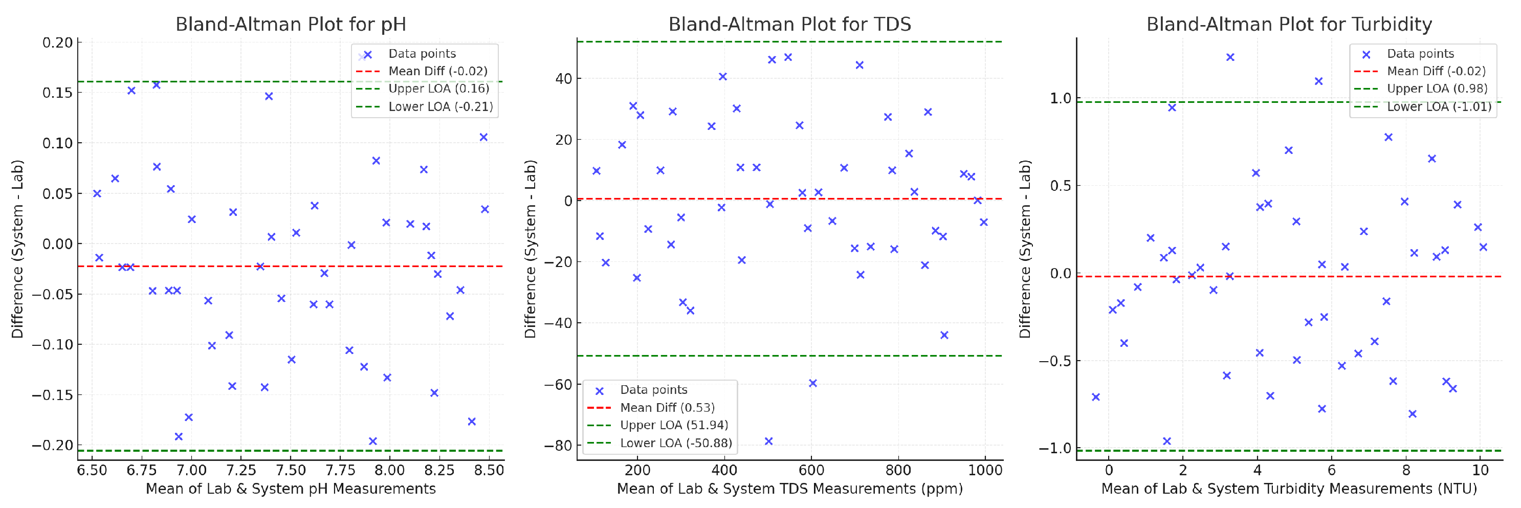
5.1.2. Bland–Altman Analysis
5.1.3. Results and Interpretation
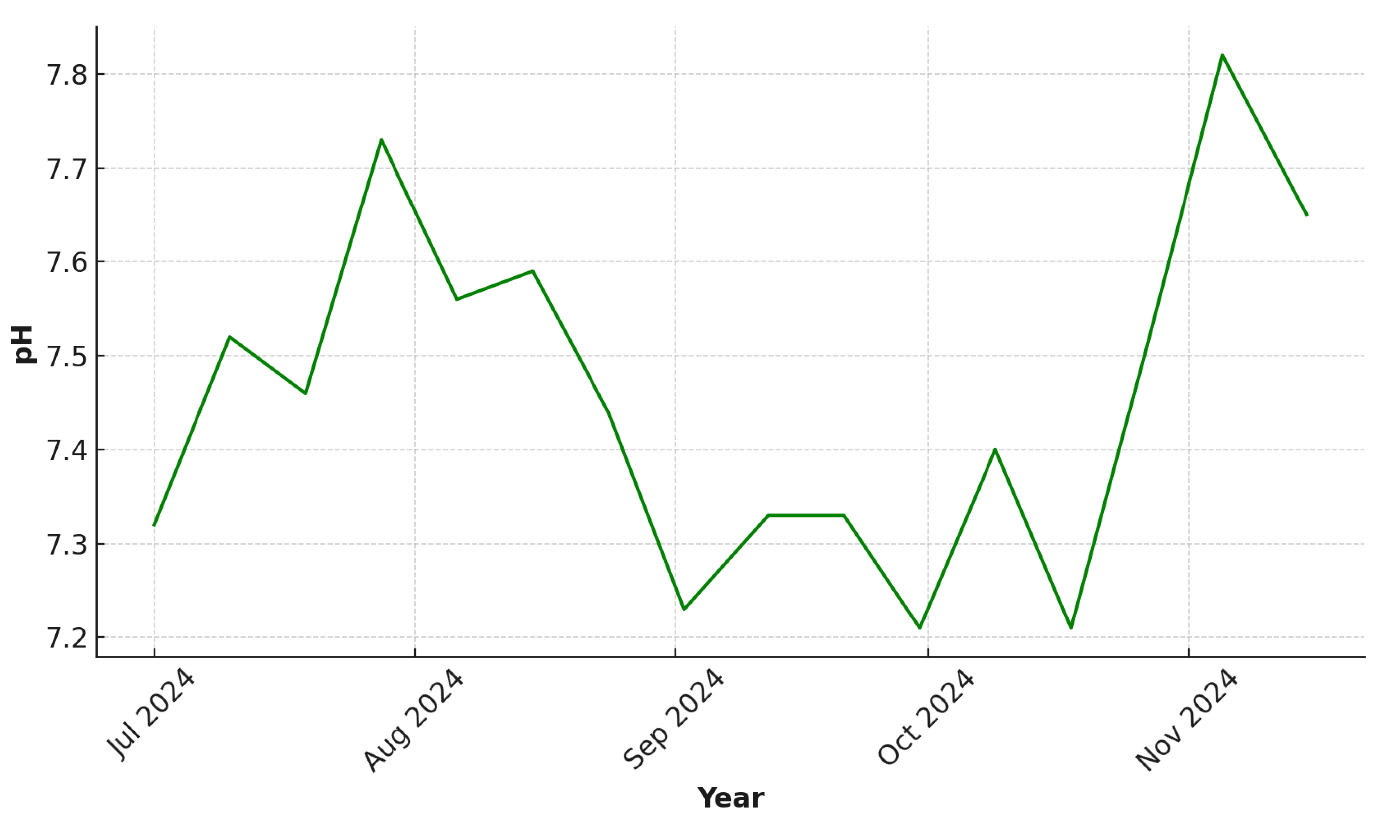
- pH Analysis:The mean difference () is close to 0.00, with LOA within pH, indicating minimal systematic bias and high consistency across the measurement range.
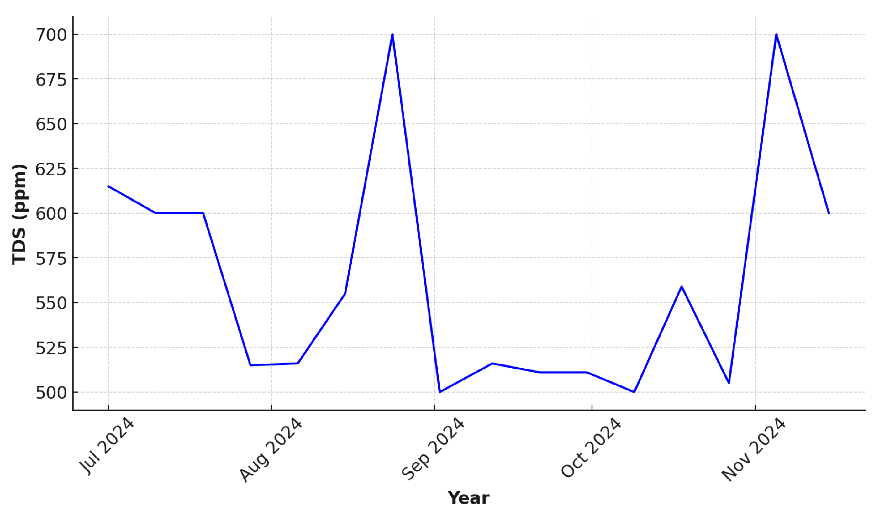
- TDS Analysis: The system measurements show a slightly positive bias, with values 5–10 ppm higher than laboratory readings, particularly at higher concentrations (>800 ppm). The LOA extends to ppm, suggesting minor discrepancies due to sensor non-linearity at elevated TDS levels.
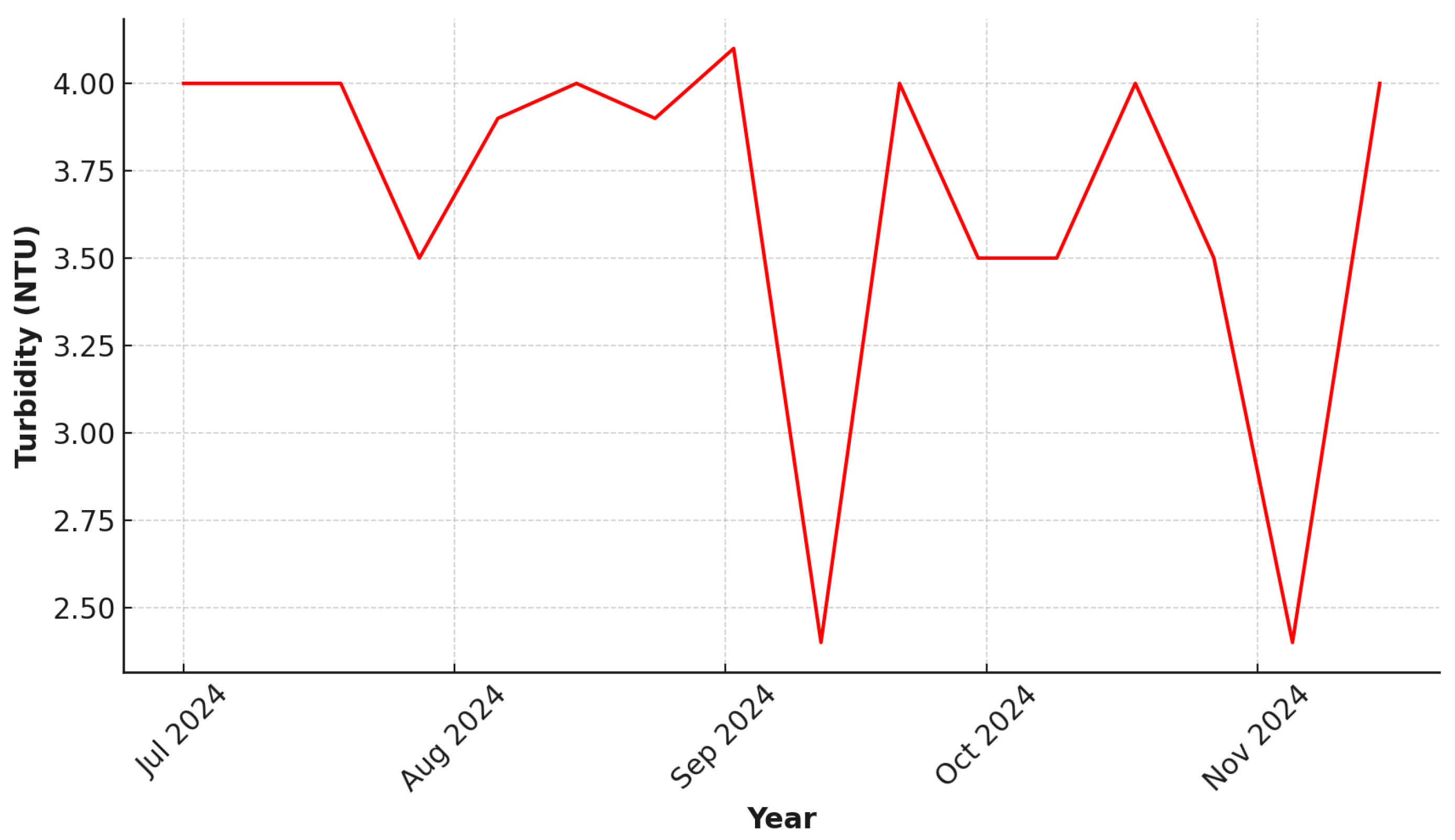
- Turbidity Analysis: The mean difference is 0.1 NTU, with LOA at NTU, consistent with WHO drinking water standards (<5 NTU). However, higher variance near 0 NTU indicates that measurements in ultra-low-turbidity conditions may be affected by sensor noise or light scattering effects.
5.1.4. Comparison with Standard Laboratory Methods
5.2. Data Validation Through Anomaly Detection Algorithms
5.2.1. Isolation Forest
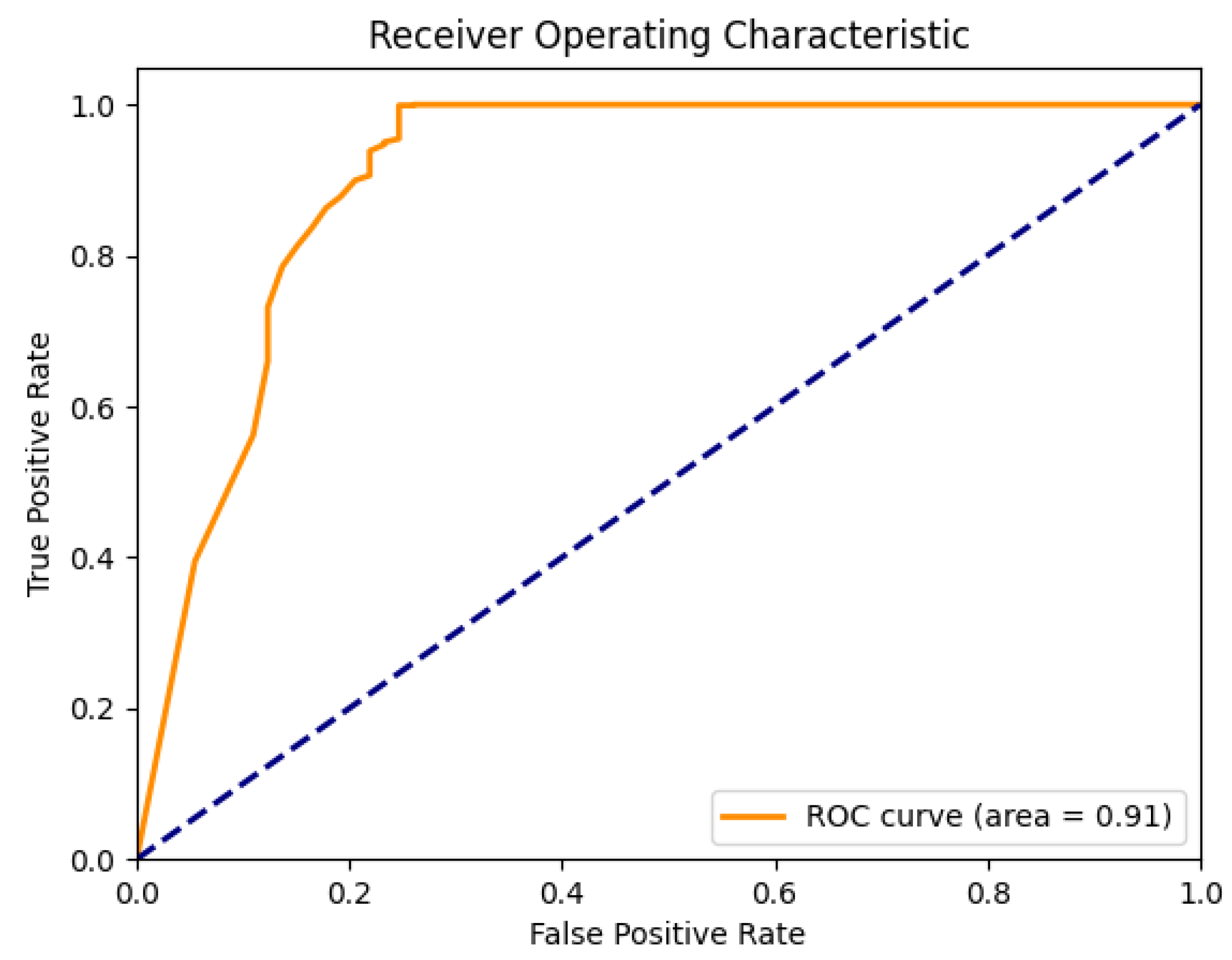
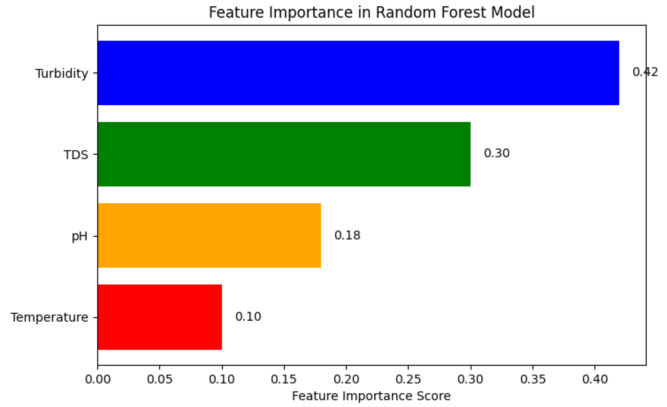
5.2.2. Random Forest
- Turbidity: 0.42;
- TDSs (total dissolved solids): 0.30;
- pH: 0.18;
- Temperature: 0.10.
5.2.3. Logistic Regression
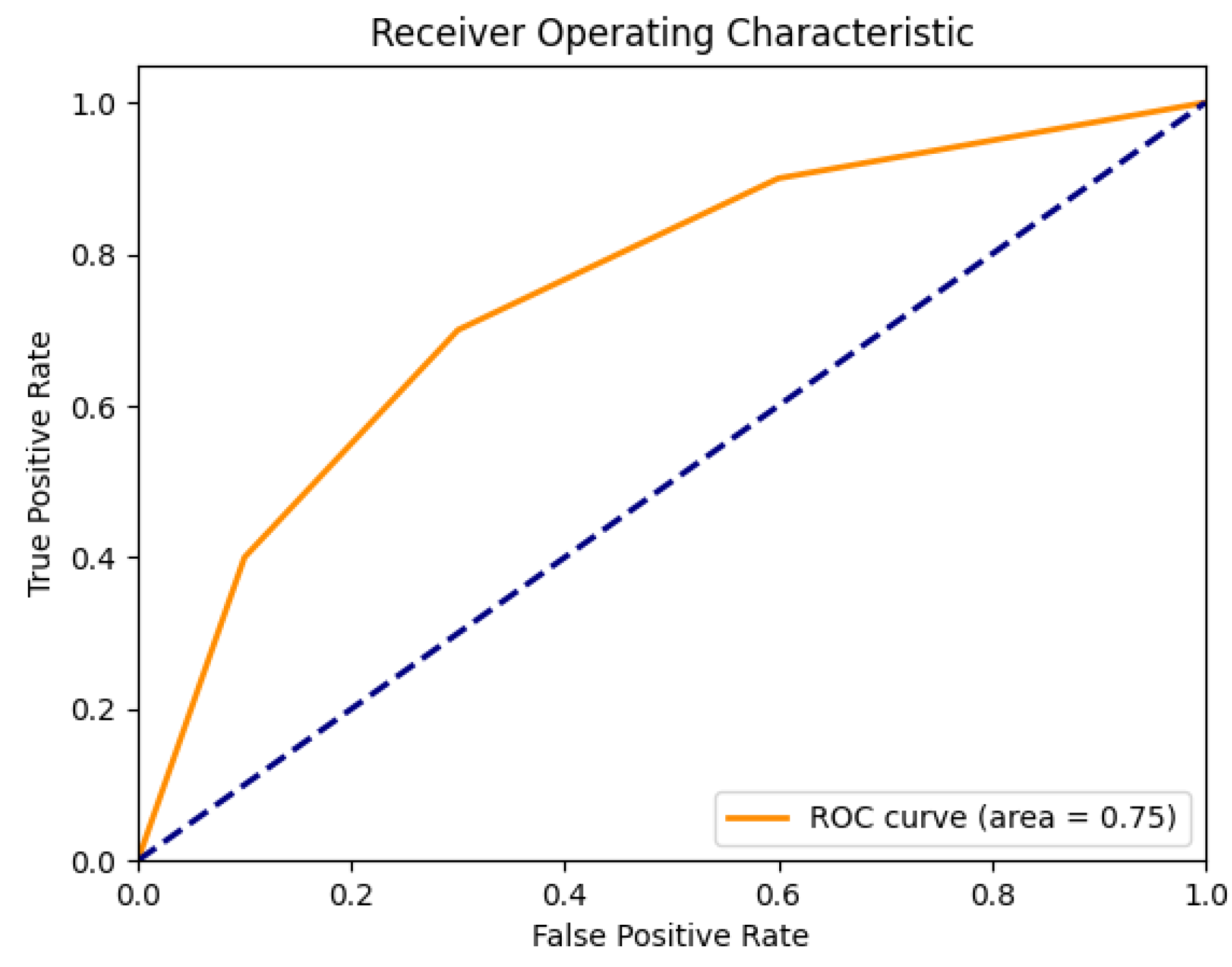
5.2.4. Local Outlier Factor
5.3. Model Evaluation and Performance
Evaluation Metrics for Anomaly Detection
- Precision [32]: Represents the proportion of truly anomalous samples among all the samples predicted as anomalous by the model. A higher precision indicates that the model is reliable in detecting anomalies, minimizing false positives.
- F1 Score [33]: The weighted average of precision and recall, particularly useful for imbalanced data situations. A higher F1 score indicates the model’s stronger stability in anomaly detection.
- Accuracy: Measures the proportion of correctly classified samples in the entire dataset. However, for anomaly detection tasks, accuracy is not the best evaluation metric as normal data usually dominate the dataset.
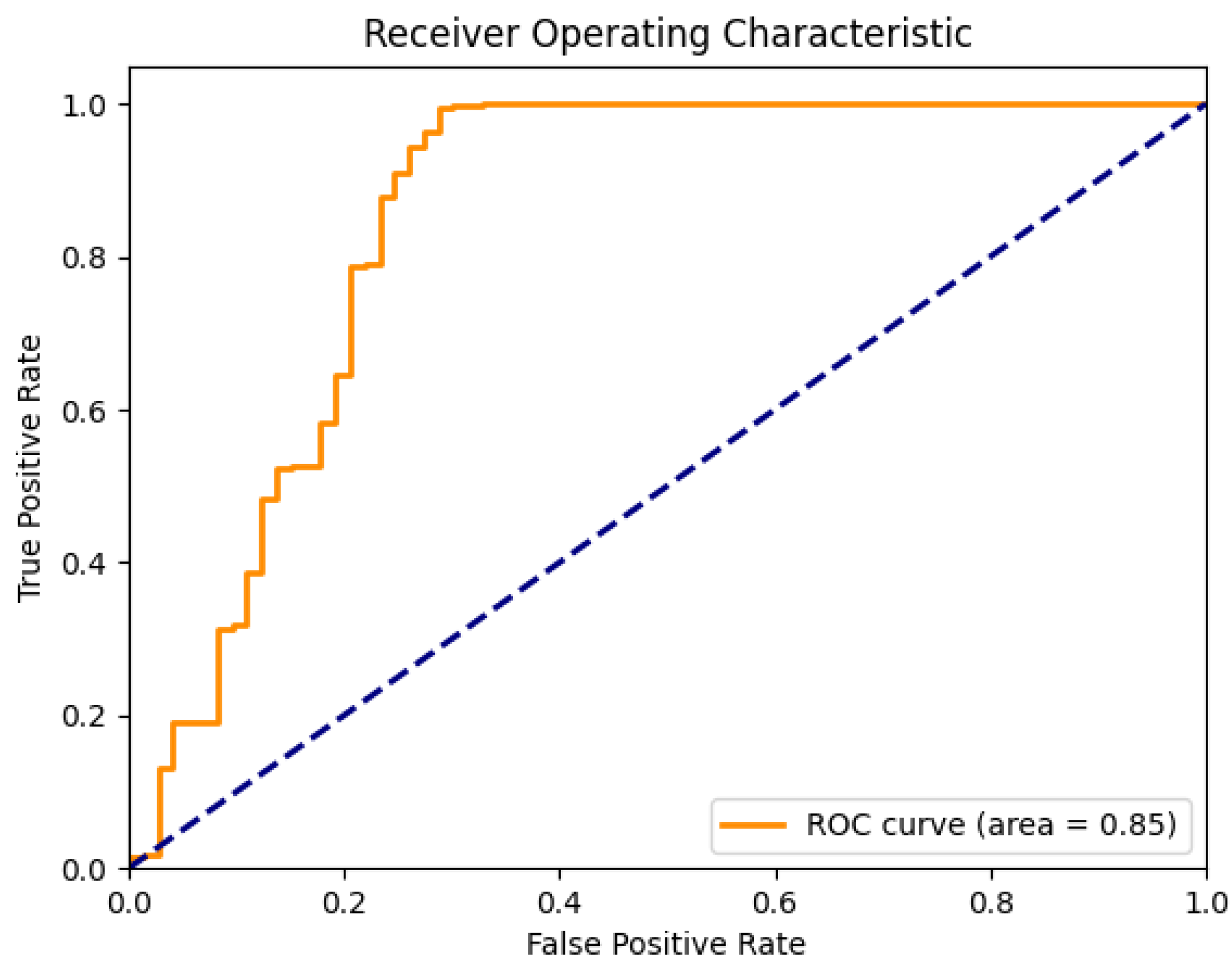
- AUC-ROC (Area Under the Curve of Receiver Operating Characteristic) [34]: Measures the model’s ability to distinguish between normal and anomalous data. An AUC close to 1.0 indicates that the model has strong discriminative power and can effectively detect water quality anomalies.
6. Conclusions
Author Contributions
Funding
Institutional Review Board Statement
Informed Consent Statement
Data Availability Statement
Conflicts of Interest
References
- Marine and Water Bureau of Macao Special Administrative Region. Water Quality Information; Marine and Water Bureau of Macao Special Administrative Region: Macao, China, 2025. [Google Scholar]
- Zhan, S.; Zhou, B.; Li, Z.; Li, Z.; Zhang, P. Evaluation of source water quality and the influencing factors: A case study of Macao. Phys. Chem. Earth Parts a/b/c 2021, 123, 103006. [Google Scholar] [CrossRef]
- Homagai, P.L.; Rayamajhi, S.; Dhami, D.; Shrestha, R.L.; Bhattarai, D.P. Comparative adsorption behavior of malachite green dye onto charred and aminated sal (shorea robusta) sawdust from aqueous solution. Nepal J. Sci. Technol. 2022, 21, 81–90. [Google Scholar]
- Babatunde, A. A study on traditional water quality assessment methods. Risk Assess. Manag. Decis. 2024, 1, 41–52. [Google Scholar]
- Saravanan, A.; Kumar, P.S.; Jeevanantham, S.; Karishma, S.; Tajsabreen, B.; Yaashikaa, P.; Reshma, B. Effective water/wastewater treatment methodologies for toxic pollutants removal: Processes and applications towards sustainable development. Chemosphere 2021, 280, 130595. [Google Scholar]
- Dutta, S.; Sarma, D.; Nath, P. Ground and river water quality monitoring using a smartphone-based pH sensor. Aip Adv. 2015, 5, 057151. [Google Scholar]
- Aluwong, K.C.; Mohd Hashim, M.H.B.; Ishmail, S. Design of wireless-based sensor for real-time monitoring pH and TDS in Surface and Groundwater using IoT. J. Min. Environ. 2024, 15, 1309–1320. [Google Scholar]
- Koestoer, R.; Saleh, Y.; Roihan, I.; Harinaldi, H. A simple method for calibration of temperature sensor DS18B20 waterproof in oil bath based on Arduino data acquisition system. AIP Conf. Proc. 2019, 2062, 020006. [Google Scholar]
- Mylvaganaru, S.; Jakobsen, T. Turbidity sensor for underwater applications. In Proceedings of the IEEE Oceanic Engineering Society. OCEANS’98. Conference Proceedings, Nice, France, 28 September–1 October 1998; Volume 1, pp. 158–161. [Google Scholar]
- Walden, R.H. Analog-to-digital converter survey and analysis. IEEE J. Sel. Areas Commun. 1999, 17, 539–550. [Google Scholar] [CrossRef]
- Peña, E.; Legaspi, M.G. UART: A hardware communication protocol understanding universal asynchronous receiver/transmitter. Visit Analog 2020, 54, 1–5. [Google Scholar]
- Fonseca-Campos, J.; Reyes-Ramirez, I.; Guzman-Vargas, L.; Fonseca-Ruiz, L.; Mendoza-Perez, J.A.; Rodriguez-Espinosa, P. Multiparametric system for measuring physicochemical variables associated to water quality based on the Arduino platform. IEEE Access 2022, 10, 69700–69713. [Google Scholar] [CrossRef]
- World Health Organization. Available online: https://www.who.int/ (accessed on 4 March 2025).
- Parry, R. Agricultural phosphorus and water quality: A US Environmental Protection Agency perspective. J. Environ. Qual. 1998, 27, 258–261. [Google Scholar]
- Li, Y.; Mao, Y.; Xiao, C.; Xu, X.; Li, X. Flexible pH sensor based on a conductive PANI membrane for pH monitoring. RSC Adv. 2020, 10, 21–28. [Google Scholar]
- Adjovu, G.E.; Stephen, H.; James, D.; Ahmad, S. Measurement of total dissolved solids and total suspended solids in water systems: A review of the issues, conventional, and remote sensing techniques. Remote Sens. 2023, 15, 3534. [Google Scholar] [CrossRef]
- Ma’ruf, K.; Setiawan, R.J.; Alam, A.A.K.; Ismail, T.; Muhammad, C.I.; Ali, J. Internet of Things for Real-Time Monitoring of Water Quality with Integrated Temperature, pH, and TDS Sensors. In Proceedings of the 2024 International Conference on Electrical Engineering and Computer Science (ICECOS), Palembang, Indonesia, 25–26 September 2024; pp. 314–319. [Google Scholar]
- Jamil, A.; Ting, T.S.; Abidin, Z.Z.; Othman, M.; Wahab, M.H.A.; Abdullah, M.F.L.; Homam, M.J.; Audah, L.H.M.; Shah, S.M. Polynomial Regression Calibration Method of Total Dissolved Solids Sensor for Hydroponic Systems. Pertanika J. Sci. Technol. 2023, 31, 2769–2782. [Google Scholar]
- Matos, T.; Martins, M.; Henriques, R.; Goncalves, L. A review of methods and instruments to monitor turbidity and suspended sediment concentration. J. Water Process. Eng. 2024, 64, 105624. [Google Scholar]
- Jingzhuo, W.; Chenglong, G. Research on 1-wire bus temperature monitoring system. In Proceedings of the 2007 8th International Conference on Electronic Measurement and Instruments, Xi’an, China, 16–18 August 2007; pp. 3–722. [Google Scholar]
- Jordán-Cuebas, F.; Krogmann, U.; Andrews, C.; Senick, J.; Hewitt, E.; Wener, R.; Sorensen Allacci, M.; Plotnik, D. Understanding apartment end-use water consumption in two green residential multistory buildings. J. Water Resour. Plan. Manag. 2018, 144, 04018009. [Google Scholar]
- Ghoneim, M.; Nguyen, A.; Dereje, N.; Huang, J.; Moore, G.; Murzynowski, P.; Dagdeviren, C. Recent progress in electrochemical pH-sensing materials and configurations for biomedical applications. Chem. Rev. 2019, 119, 5248–5297. [Google Scholar]
- Shehata, A.B.; AlAskar, A.R.; Al Dosari, R.A.; Al Mutairi, F.R. Calibration and ISO GUM Based Uncertainty of Conductivity and TDS Meters for Better Water Quality Monitoring. Sci. J. Chem. 2022, 10, 211–218. [Google Scholar]
- Trevathan, J.; Read, W.; Sattar, A. Implementation and calibration of an IoT light attenuation turbidity sensor. Internet Things 2022, 19, 100576. [Google Scholar]
- Edition, F. Guidelines for drinking-water quality. WHO Chron. 2011, 38, 104–108. [Google Scholar]
- Wei, Y.; Hu, D.; Ye, C.; Zhang, H.; Li, H.; Yu, X. Drinking water quality & health risk assessment of secondary water supply systems in residential neighborhoods. Front. Environ. Sci. Eng. 2024, 18, 18. [Google Scholar]
- Giavarina, D. Understanding bland altman analysis. Biochem. Medica 2015, 25, 141–151. [Google Scholar]
- Liu, F.T.; Ting, K.M.; Zhou, Z.H. Isolation forest. In Proceedings of the 2008 Eighth Ieee International Conference on Data Mining, Pisa, Italy, 15–19 December 2008; IEEE: Pisa, Italy, 2008; pp. 413–422. [Google Scholar]
- Rigatti, S.J. Random forest. J. Insur. Med. 2017, 47, 31–39. [Google Scholar] [CrossRef]
- LaValley, M.P. Logistic regression. Circulation 2008, 117, 2395–2399. [Google Scholar]
- Alghushairy, O.; Alsini, R.; Soule, T.; Ma, X. A review of local outlier factor algorithms for outlier detection in big data streams. Big Data Cogn. Comput. 2020, 5, 1. [Google Scholar] [CrossRef]
- Streiner, D.L.; Norman, G.R. “Precision” and “accuracy”: Two terms that are neither. J. Clin. Epidemiol. 2006, 59, 327–330. [Google Scholar]
- Yacouby, R.; Axman, D. Probabilistic extension of precision, recall, and f1 score for more thorough evaluation of classification models. In Proceedings of the First Workshop on Evaluation and Comparison of NLP Systems, Online, 20 November 2020; pp. 79–91. [Google Scholar]
- Narkhede, S. Understanding auc-roc curve. Towards Data Sci. 2018, 26, 220–227. [Google Scholar]


| Sensor Type | Model | Accuracy | Sensitivity | Price | Power Consumption | Calibration Cycle |
|---|---|---|---|---|---|---|
| pH | Atlas Scientific EZO-pH | ±0.002 | High | High | Low | 4–6 weeks |
| pH | DFROBOT SEN0161-V2 | ±0.1 | Medium | Low | Low | 2–4 weeks |
| pH | pH-4502C | ±0.02 | Medium | Medium | Medium | 2–3 weeks |
| TDS | Atlas Scientific EZO-EC | ±2% | High | High | Low | 4–6 weeks |
| TDS | DFROBOT Gravity TDS | ±10% | Medium | Low | Low | 2–4 weeks |
| Turbidity | In Situ Aqua TROLL 200 | ±0.1 NTU | High | High | Low | 8 weeks |
| Turbidity | DFROBOT SEN0189 | ±3% | Medium | Low | Low | 4 weeks |
| Temperature | DS18B20 (Digital) | ±0.5 °C | High | Low | Low | 6 months |
| Temperature | PT100 (Analog) | ±0.1 °C | High | High | High | 6 months |
| Parameter | WHO Guideline | EPA Drinking Water Standard | GB 5749-2022 (China Standard) | Unit |
|---|---|---|---|---|
| pH | - | |||
| TDS | ≤1000 | ≤500 (recommended) | ≤1000 | mg/L |
| Turbidity | ≤5 (short-term maximum) | ≤1 (95% sample value) | ≤1 | NTU |
| Temperature | No strict standard | No strict standard | No strict standard | °C |
| Parameter | Condition | Score |
|---|---|---|
| TDS (ppm) | TDS ≤ 500 | 1 |
| 500 < TDS ≤ 1000 | 0.5 | |
| TDS > 1000 | 0 | |
| pH | 6.5 ≤ pH ≤ 8.5 | 1 |
| 6.0 ≤ pH < 6.5 or 8.5 < pH ≤ 9.0 | 0.5 | |
| pH < 6.0 or pH > 9.0 | 0 | |
| Temperature (°C) | Temperature ≤ 15 | 1 |
| 15 ≤ Temperature < 25 | 0.5 | |
| Temperature > 25 | 0 | |
| Turbidity (NTU) | Turbidity ≤ 5 | 1 |
| 5 < Turbidity ≤ 10 | 0.5 | |
| Turbidity > 10 | 0 |
| Overall Score | Label | Explanation |
|---|---|---|
| 1.0 | Meets Physicochemical Criteria (1) | Falls within all optimal physicochemical limits. |
| 0.5 ≤ Score < 1.0 | Borderline Condition (0.5) | Partially acceptable but does not fully meet optimal criteria. |
| Score < 0.5 | Does Not Meet Physicochemical Criteria (0) | Fails to meet the minimum physicochemical standards. |
| Model | Precision | F1 Score | Accuracy | AUC |
|---|---|---|---|---|
| Isolation Forest | 97.7% | 98.56% | NA | 0.85 |
| Random Forest | 97.99% | 98.99% | 98.10% | 0.91 |
| Logistic Regression | 96.76% | 98.36% | 96.90% | 0.86 |
| Local Outlier Factor | 93.54% | 96.66% | NA | 0.75 |
Disclaimer/Publisher’s Note: The statements, opinions and data contained in all publications are solely those of the individual author(s) and contributor(s) and not of MDPI and/or the editor(s). MDPI and/or the editor(s) disclaim responsibility for any injury to people or property resulting from any ideas, methods, instructions or products referred to in the content. |
© 2025 by the authors. Licensee MDPI, Basel, Switzerland. This article is an open access article distributed under the terms and conditions of the Creative Commons Attribution (CC BY) license (https://creativecommons.org/licenses/by/4.0/).
Share and Cite
Gao, J.; Chen, B.; Tang, S.-K. Water Quality Monitoring: A Water Quality Dataset from an On-Site Study in Macao. Appl. Sci. 2025, 15, 4130. https://doi.org/10.3390/app15084130
Gao J, Chen B, Tang S-K. Water Quality Monitoring: A Water Quality Dataset from an On-Site Study in Macao. Applied Sciences. 2025; 15(8):4130. https://doi.org/10.3390/app15084130
Chicago/Turabian StyleGao, Jiawei, Bochao Chen, and Su-Kit Tang. 2025. "Water Quality Monitoring: A Water Quality Dataset from an On-Site Study in Macao" Applied Sciences 15, no. 8: 4130. https://doi.org/10.3390/app15084130
APA StyleGao, J., Chen, B., & Tang, S.-K. (2025). Water Quality Monitoring: A Water Quality Dataset from an On-Site Study in Macao. Applied Sciences, 15(8), 4130. https://doi.org/10.3390/app15084130