Machine-Learning-Based Integrated Mining Big Data and Multi-Dimensional Ore-Forming Prediction: A Case Study of Yanshan Iron Mine, Hebei, China

Abstract

With the rapid development of big data and artificial intelligence technologies, the era of Industry 4.0 has driven large open-pit mines towards digital and intelligent transformation. This is particularly true in mature mining areas such as the Yanshan Iron Mine, where the depletion of shallow proven reserves and the increasing issues of mixed surrounding rocks with shallow ore bodies make it increasingly important to build intelligent mines and implement green and sustainable development strategies. However, previous mineralization predictions for the Yanshan Iron Mine largely relied on traditional geological data (such as blasting rock powder, borehole profiles, etc.) exploration reports or three-dimensional explicit ore body models, which lacked precision and were insufficient to meet the requirements for intelligent mine construction. Therefore, this study, based on artificial intelligence technology, focuses on geoscience big data mining and quantitative prediction, with the goal of achieving multi-scale, multi-dimensional, and multi-modal precise positioning of the Yanshan Iron Mine and establishing its intelligent mine technology system. The specific research contents and results are as follows: (1) This study collected and organized multi-source geoscience data for the Yanshan Iron Mine, including geological, geophysical, and remote sensing data, such as mine drilling data, centimeter-level drone image data, and high-spectral data of rocks and minerals, establishing a rich mine big data set. (2) SOM clustering analysis was performed on the elemental data of rock and mineral samples, identifying key elements positively correlated with iron as Mg, Al, Si, S, K, Ca, and Mn. TSG was used to interpret shortwave and thermal infrared hyperspectral data of the samples, identifying the main alteration mineral types in the mining area. Combined with spectral and elemental analysis, the universality of alteration features such as chloritization and carbonation, which are closely related to the mineralization process, was further verified. (3) Based on the spectral and elemental grade data of rock and mineral samples, a training model for ore grade–spectrum correlation was constructed using Random Forests, Support Vector Machines, and other algorithms, with the SMOTE algorithm applied to balance positive and negative samples. This model was then applied to centimeter-level drone images, achieving high-precision intelligent identification of magnetite in the mining area. Combined with LiDAR image elevation data, a real-time three-dimensional surface mineral monitoring model for the mining area was built. (4) The Bagged Positive Label Unlabeled Learning (BPUL) method was adopted to integrate five evidence maps—carbonate alteration, chloritization, mixed rockization, fault zones, and magnetic anomalies—to conduct three-dimensional mineralization prediction analysis for the mining area. The locations of key target areas were delineated. The SHAP index and three-dimensional explicit geological models were used to conduct an in-depth analysis of the contributions of different feature variables in the mineralization process of the Yanshan Iron Mine. In conclusion, this study successfully constructed the technical framework for intelligent mine construction at the Yanshan Iron Mine, providing important theoretical and practical support for mineralization prediction and intelligent exploration in the mining area.

1. Introduction

Iron ore is one of the indispensable resources in the world, playing a key role in the development of various sectors such as metallurgy, chemicals, construction, transportation, and machinery. China is a major energy-consuming country, and although it possesses abundant iron ore reserves, the country’s resources cannot fully meet domestic demand due to a low ore grade and mining technology limitations. As a result, most of the high-grade iron ore resources are still reliant on imports, with China accounting for more than 60% of global iron ore imports [1]. The Yanshan Iron Ore Mine is part of the giant Sijia Ying ore deposit and, like other iron ore deposits in the eastern Hebei region, is large in scale, but characterized by low-grade ores and long mining histories. These deposits are facing the issue of exhausted proven mineral reserves, making it urgent to explore deeper ore potentials [2,3]. Moreover, the Yanshan ore deposit is complex in terms of ore body distribution, with many intercalated rocks and unclear boundaries between ore bodies and surrounding rocks, leading to the challenge of low iron ore recovery.

Currently, the main task of mineral resource quantitative prediction is to establish metallogenic models based on the comprehensive analysis of multi-source geoscientific information, including geology, geophysics, geochemistry, and remote sensing. This process involves constructing mathematical models, extracting and identifying favorable mineralization information, and conducting data fusion to create mineral prediction models. These models are used for the quantitative evaluation of potential mineral resources and to delineate exploration targets [3]. Integrating geoscience data from different dimensions, types, and scales for comprehensive analysis and modeling also helps geologists effectively identify geological backgrounds, metallogenic characteristics, and exploration directions. With the continuous development of real-time monitoring technologies such as “Sky–Earth–Deep” multi-scale multi-scenario observations and 5G+ communication, geoscience big data have undergone significant advancements and innovations, providing opportunities for the development of machine learning in the field of Earth sciences. This is particularly true in areas such as mineral exploration [4,5,6], remote sensing image analysis [7,8,9], and geological disaster prediction and risk assessment [10,11,12]. Nowadays, with the widespread acceptance of the concept of green sustainable development, the construction of intelligent mines under the integrated management of “resources–environment–economy” has become mainstream. In addition, considering the existing issues in deposits like the Yanshan Iron Ore Mine, the use of multi-source geoscience big data combined with methods like machine learning for quantitative prediction of mineral resources in mining areas has become crucial. Machine learning has been widely applied in various fields of mineral quantitative prediction research, achieving remarkable results, including in remote sensing alteration interpretation [13,14,15], three-dimensional/four-dimensional mineralization prediction [16,17,18,19,20], element grade analysis [21,22], and environmental monitoring of mining areas [23].

Machine learning is divided into two categories: data-driven and knowledge-driven. Data-driven approaches include supervised, unsupervised, and semi-supervised learning, which use the locations of known mineral occurrences as labeled data to construct relationships between feature variables and predictive variables and employ mathematical methods for integrated decision-making [24]. Knowledge-driven approaches, on the other hand, are based on expert knowledge to assign weights to feature variables for decision-making, being suitable for targets with no or few known occurrences [25]. In recent years, with the exponential increase in the quantity of geoscientific data, machine learning has gradually evolved towards deep learning, including techniques like convolutional neural networks [26], deep autoencoders [27], generative adversarial networks [28], and restricted Boltzmann machines [29] that leverage their mechanisms to capture high-dimensional data features from massive geoscientific datasets [30]. Luo has proposed a comprehensive geochemical data analysis framework using a causal discovery algorithm and a hybrid deep learning model of VAE-CAPSNET-GAN, effectively identifying geochemical anomaly areas related to mineralization [31]. Deng used Laplace–Beltrami eigenfunctions, surface normals, and surface distances to describe the geological boundaries of predictive variables and organized them into multi-channel images through perspective projection, combined with a CNN architecture to perform three-dimensional mineralization prediction assessments [32]. Under the precondition of accuracy, interpretability, and physical reality of machine learning algorithms applied to geoscientific applications, the features of geoscientific systems and data [33], including their multi-source and multi-scale nature, auto-correlation and cross-correlation, and spatiotemporal heterogeneity, have been fully demonstrated [34,35]. Luo explored the contributions of geochemical elements in identifying multivariate geochemical anomalies using the SHAP explainability framework and variational autoencoder models [36]. Zhang proposed a BPUL structure integrated framework to address system uncertainties caused by imbalanced data and cost-sensitive issues in data-driven machine learning algorithms [37].

This study aims to address issues such as ore–rock mixing and depletion of deep reserves by integrating and constructing a multi-source geoscientific dataset, including geological data (such as drilling data, geological profiles, and geological topographic maps), geophysical data (aerial magnetic survey data based on drones), geochemical data (XRF trace element detection data from mining area samples), and remote sensing data (drone digital elevation data, drone LiDAR images, and drone multispectral imaging). Using big data and artificial intelligence methods, this study conducts mining big data integration analysis and knowledge discovery from multiple dimensions and modalities, performing an in-depth analysis of the geological genesis of the deposit. The goal is to accurately locate the surface and deep potential ore bodies in the study area, achieve real-time detection of surface ore bodies in the Yanshan Iron Ore Mine open-pit mining area, identify deep exploration indicators and exploration directions, and promote the development and construction of the Yanshan Iron Ore Mine as an intelligent mine. This study aims to increase production efficiency and improve iron ore recovery rates.

2. Study Area and Data

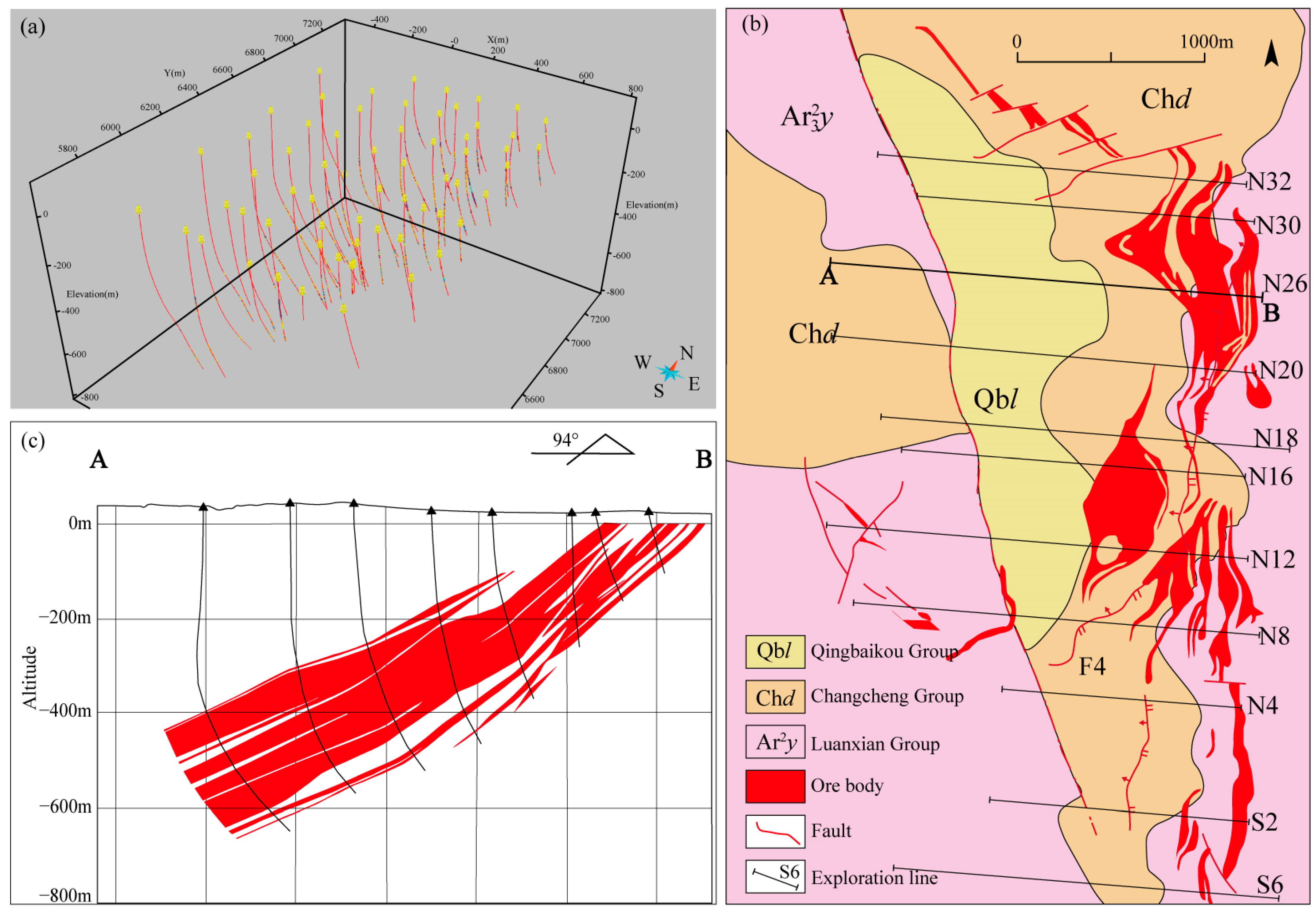
2.1. Geology Setting

The eastern Hebei area is situated in the northeastern part of the Jizhong–Jidong micro-block, which lies in the central segment of the northern margin of the North China Craton (Figure 1a) [38]. After undergoing a series of geological evolution stages, the area developed several large-scale Banded Iron Formation (BIF)-type iron ore deposits, including the Sijiaying, Macheng, Shuichang, Shirengou, Xingshan, Zuolanzhangzi, and Malanzhuang deposits [39]. This area has an estimated iron ore reserve of approximately 6.3 billion tons, and it still holds significant potential for future exploration [40]. The Yanshan iron deposit, located in the southern part of Hebei Province, China, and covering an area of approximately 4 km², is situated to the north of the N18 exploration line, which separates it from the super-large Sijiaying BIF-type iron ore deposit (Figure 1b). The Yanshan iron deposit, an Algoma-type Banded Iron Formation (BIF) deposit, experienced mineralization during the late Neoarchean. The initial source of the ore minerals was the mixing of high-temperature submarine hydrothermal fluids and seawater. Subsequently, it underwent primary sedimentation, metamorphism, multiple phases of tectonic activity, and hydrothermal alteration, ultimately resulting in the accumulation of iron-rich ores [41].

The basement stratum of the Yanshan iron deposit consists of the Neoarchean Luanxian Group, while the overlying strata of this deposit include the Mesoproterozoic to Neoproterozoic Changcheng, Jixian, and Qingbaikou systems, followed by the Cambrian, Ordovician, Carboniferous, Permian, and Quaternary systems. The Luanxian Group serves as the primary ore-hosting formation, reaching low-amphibolite facies metamorphism. The main lithologies are biotite granulite, magnetite (or hematite) quartzite, and plagioclase amphibolite [42]. After undergoing two phases of folding, the basement structure of the area is now composed of the nearly N-S trending Yangshan anticlinorium and Sima synclinorium, extending from east to west. Among them, the Sima synclinorium is larger in scale and is further divided into five subordinate folds: the Macheng synclinorium, Xinxian anticlinorium, Sijiaying synclinorium, Damazhuang anticlinorium, and Gaoguanying–Lixiazhuang synclinorium. These folds control the morphology, spatial distribution, scale, and occurrence of the major sedimentary–metamorphic iron ore deposits in the surrounding area. The ore body of the Yanshan iron deposit is thickened near the core of the fold [43]. The fault structures in the mining area are primarily a set of northeast to north-trending faults that run nearly parallel to the ore body, exhibiting a wave-like surface pattern. This compressive-shear reverse fault dips southeastward along its strike, crossing the ore body from south to north, leading to displacement along the fault and causing shifts in the position and morphology of the ore body. Magmatic activity in the area is minimal, with only small-scale pegmatite veins and segmental metamorphosed gabbro-diabase veins observed [44].

The main rock type of the Yanshan iron deposit is magnetite quartzite, while the primary ore type in the surface oxidized zone is hematite quartzite [45]. Based on geological characteristics, the high-grade iron ore in the mining area can be roughly divided into two categories [46,47]. The first type of high-grade iron ore is formed by primary sedimentation, with limited exposure, mainly found in the lower part of thick, low-grade ore bodies. The second type of high-grade iron ore is formed through hydrothermal alteration of low-grade ores. In this area, the hydrothermal alteration model is described as “desilication and iron enrichment”, occurring under high-temperature, weakly alkaline, and strongly reducing conditions. During this process, the hydrothermal fluids remove silica and some iron, while the remaining iron is enriched in situ to form high-grade iron ore. This type of high-grade ore is more widely distributed in the area, typically occurring within low-grade ore bodies in stratiform patterns consistent with the host rock. The high-grade ore is characterized by dense massive textures, with disseminated and fine-banded textures being less common, and features coarser grain sizes. Magnetite is the primary ore mineral, with less hematite present. The gangue minerals include chlorite, carbonate minerals, biotite, amphibole, feldspar, quartz, and minor pyrite [48].

2.2. Mine Big Data

Based on the geological characteristics of the Yanshan iron ore deposit, this study collects and organizes several datasets (

Table 1. Datasets of Yanshan iron deposit.

Dataset	Description	Method
Previous Geological Survey Data	Regional geological maps, geomorphological geological maps, exploration line cross-sections (11), and drilling logs (70)	3D geological modeling
Mineral Hyperspectral Data	SWIR hyperspectral data (395) and TIR hyperspectral data (134)	TSG interpretation
XRF	Major and trace elements (395)	SOM clustering
UAV Remote Sensing Imagery	LiDAR images, digital elevation data, visible light orthophotos, and multispectral imagery.	3D surface modeling, 2D intelligent identification of magnetite
UAV Aeromagnetic Survey	1:2000 UAV aeromagnetic data	Reduction to the pole, geophysical inversion

), including the following: (1) geological data from the exploration phase, such as topographic geological maps, exploration line profiles, drilling data, exploration reports, and other related materials; (2) multi-phase field rock sample collection; (3) XRF trace element data and hyperspectral (shortwave infrared, thermal infrared) data for rock and mineral samples; (4) multi-temporal unmanned aerial vehicle (UAV) image datasets, including digital elevation models (DEMs), LiDAR point cloud data, multispectral images, orthophotos, and 1:2000 aerial magnetic survey data.

2.2.1. UAS Imagery—Multispectral, LiDAR, Aeromagnetic

With the rapid development of drone technology, its application in mineral exploration has become increasingly mature and widespread, providing new directions for research and application in the fields of geological and geophysical exploration. This study used a Matrice 350 RTK drone produced by DJI (Shenzhen, Guangdong, China), equipped with multiple sensors, to acquire multi-temporal remote sensing imagery of the Yanshan iron deposit.

First, multi-temporal UAV Structure-from-Motion (UAV-SFM) aerial imagery of the mining area was captured using the Zenmuse L1 sensor produced by DJI (Shenzhen, Guangdong, China). This sensor integrates Livox LiDAR, high-precision inertial navigation (RTK), and RGB cameras, enabling all-weather, efficient, and real-time 3D data acquisition in complex environments. This allowed for the generation of high-precision 3D surface models (Figure 2a) and 2D visible light orthophotos (DOM) (Figure 3a–c). The Digital Surface Model (DSM) aids in the 3D visualization and reconstruction of the mining area [49]. The results of the Digital Surface Model (DSM) clearly reveal the surface features of the open-pit mine, including the distinct boundary between the sandstone and gravel layers and the underlying strata on the southwestern side (Figure 2b). On the northeastern side, the formation of the pit slope shows significant folding patterns in the strata (Figure 2c). In the currently mined area, the boundary between the surrounding rock (black cloud metamorphic granite) and the ore body (magnetite quartzite) is unclear under visible light. After blasting, the mixed areas of ore and rock are prone to increasing ore loss and waste rock contamination, which affects the recovery rate of iron ore (Figure 2b,d). Meanwhile, the digital orthophoto maps (Figure 3a–c) provide reference images for selecting surface sampling points [50].

Additionally, multi-temporal multispectral imaging was conducted using the MS600 Pro multispectral sensor produced by Yusense (Qingdao, Shandong, China), with a spatial resolution of 8.5 cm. The spectral bands of the sensor are as follows: Blue (450 ± 35 nm), Green (530 ± 27 nm), Red (650 ± 25 nm), Red Edge (720 ± 10 nm), Near Infrared (840 ± 26 nm), and 900 ± 35 nm. During the flight, the aircraft captured images at an altitude of 80 m AGL along the flight path, ensuring a 75% forward overlap and 65% side overlap, while the RTK system provided precise positioning. Finally, Yusense Map was used for image registration, stitching, and radiometric calibration, generating high-precision multi-temporal UAV multispectral imagery (Figure 4). Figure 4a–c show the false-color composite results of multispectral imagery for the mining area for three different periods (Red: 650 ± 25 nm, Green: 530 ± 27 nm, Blue: 450 ± 35 nm). When combined with the digital orthophoto maps (true-color images from different periods shown in Figure 3a–c), they further confirm the complexity of visually interpreting the ore body (magnetite quartzite) and surrounding rock (black cloud metamorphic granite) within the visible light range. This highlights the need for a series of subsequent processing steps to effectively delineate the surface ore and rock.

Finally, we conducted a UAV airborne magnetic anomaly survey in the mining area using the rubidium vapor magnetometer which is produced by QuSpin Inc. (Louisville, CO, USA). The magnetometer has a sampling range of 1000–100,000 nT and a maximum sampling rate of 400 Hz and records GPS data at a frequency of 20 Hz. During the flight, the magnetometer was securely mounted on the side of the UAV, with its axis parallel and perpendicular to the UAV’s main axis, maintaining an altitude of 80 m AGL for airborne measurements.

To eliminate the effects of diurnal variations during magnetic surveys, a magnetic base station was established at a location over 100 m away from the mining area to avoid the influence of external magnetic field changes on the recorded data. We calculated the total magnetic field B_t and used its variations to correct the UAV-borne total magnetic field data. Additionally, we computed the International Geomagnetic Reference Field (IGRF) for the area, which indicated a background field of approximately 53,973.053 nT, with a declination of about −7.698° and an inclination of approximately 58.565°.

Using the Geosoft Oasis Montaj 8.4.1, we applied preprocessing operations to the UAV magnetic survey data, including diurnal variation correction, polarity reversal, and RTP filtering. The magnetic anomaly data after polarity reversal were then subjected to ordinary kriging interpolation, with results shown in Figure 5. Finally, the magnetic susceptibility parameter ranges for the main lithologies and strata in the Yanshan Iron Mine area were collected and tabulated, as shown in

Table 2. Range and average values of magnetic susceptibility for the main stratigraphy/lithology of the Yanshan iron ore deposit.

Strata/Lithology	Magnetic Susceptibility
	K (10−64ΠSI)	Jr (10−3 A/m)
Quaternary	0	0
Changcheng Group	0–300	0–200
Migmatite	0–500	0–200
Biotite Granulite	0–100	0–100
Magnetite Quartzite	30,000–150,000	5000–40,000

.

Based on the magnetic susceptibility range table for the main lithologies and strata in the Yanshan Iron Mine area, along with the polarity-reversed interpolated UAV magnetic imagery (as shown in Figure 5), it was observed that the magnetic susceptibility of the main ore (magnetite quartzite) ranges from 30,000 to 150,000 (10⁻⁶⁴πSI), which is significantly higher than the magnetic susceptibility of the surrounding lithologies and strata. At the same time, the boundary between the ore body and the surrounding rocks is very distinct. Therefore, the magnetic characteristics can serve as an effective indicator to delineate the size and distribution contour of the Yanshan iron ore deposit.

Different types of sensors can acquire multi-modal lightweight UAV remote sensing image data of the mining area, forming a multi-source aerial survey dataset of the open-pit mine to provide data for subsequent two-dimensional surface magnetite intelligent recognition and three-dimensional ore-forming prediction. The key data parameters of each type of UAV image are summarized as shown in

Table 3. Key parameters for different types of lightweight UAV images.

MS600 Pro		LiDAR		QuSpin Rb OPM
Effective pixels	1.2 million	Measuring range	450 m@80%, 0 klx; 190 m@10%, 100 klx	Resolution	0.1 nT
FOV	Horizontal: 49.6°; vertical: 38°	Ranging accuracy	±2 cm (at 50 m)	Baseline error (200 Hz sampling)	3 nT
Typical width	110 m × 83 m@h = 120 m	Point cloud density	240,000 points/s	Weight	1.2 kg
Ground spatial resolution	8.65 cm@h = 120 m	FOV	Horizontal: 70.4°; vertical: 4.5°	Power Consumption	<10 w
Band range	450 nm@35 nm; 530 nm@27 nm; 650 nm@25 nm; 720 nm@10 nm; 840 nm@30 nm; 900 nm@35 nm	Positioning accuracy (IMU)	Horizontal: ~5 cm; Vertical: ~10 cm

.

2.2.2. Surface Sample Data—XRF, Spectroscopy, Susceptibility, Sampling

In this study, three phases of sample collection were conducted in April 2023, August 2023, and May 2024. In the first phase, a total of 39 samples were collected, distributed across the F4 fault zone, the northeastern and western mid-segments, and the most recent mining areas. The second phase involved the collection of 337 samples, primarily located in the newly mined areas of the mining district. In the third phase, 23 samples were collected, mainly from the ore body, ore–rock mixed zones, and surrounding rocks. The spatial distribution and frequency distribution of the samples for all three time periods are shown in Figure 3. Overall, the samples from all three stages were distributed around and near the ore body, with generally low ore grades. The iron grade is typically between 10% and 20%.

Subsequently, these samples were tested using shortwave infrared spectroscopy (SWIR), thermal infrared spectroscopy (TIR), and X-ray fluorescence (XRF), obtaining spectra for the samples.

The shortwave infrared reflectance spectra were obtained using the OreXpress^TM device produced by Spectral Evolution (Haverhill, MA, USA). The instrument has an effective testing wavelength range of 350 to 2500 nm and provides a good signal-to-noise ratio. The preparation of spectral samples requires the surface to be clean and dry, and each spectrum was acquired 3–5 times under the same conditions. The spectrometer features a sampling bandwidth of 1 nm and a minimum scanning speed of 100 ms. During sample testing with the contact probe of this device, the proprietary DARWin SP 1.4 was used for spectral recording. This software includes spectral libraries from the USGS and the SpecMIN mineral library, enabling spectral matching of samples and real-time mineral identification [51]. A total of 395 SWIR spectra from rock mineral samples were obtained for this study. Mineral spectral identification was conducted using the TSA algorithm in TSG 8.0, which matched the shape of the spectral curves and the positions of absorption peaks with those in the spectral library to determine mineral types and extract spectral information. The TSA algorithm generates a report explaining the spectral information, typically including individual minerals or mineral combinations, as well as spectral weight or estimated spectral abundance of minerals [52].

The thermal infrared reflectance spectra were determined using the Agilent 4300 handheld Fourier transform infrared spectrometer, designed and manufactured by Agilent Technologies (Santa Clara, CA, USA). This instrument weighs 2.2 kg and is equipped with a diffuse reflectance sampling module, allowing measurements over a wavelength range of 4000 to 650 cm⁻¹ (approximately 2500 to 16,000 nm) with a spectral resolution range of 4 to 16 cm⁻¹. The instrument includes MicroLab 5.7 for the storage and transmission of data, methods, and spectral libraries, and a total of 134 TIR spectral data from rock mineral samples were obtained. Since TSG 8.0 contains over 500 mineral spectra ranging from VIR to TIR, the TSA algorithm was subsequently used for mineral identification [53].

We used a portable XRF-OX44 manufactured by Fluka (Buchs, St. Gallen, Switzerland) to scan rock and mineral samples, with each sample scanned 3–5 times for 60 s per scan. After obtaining data on the major and trace element content data for 395 samples and excluding elements with a detection rate of less than 20%, we identified 23 key elements related to the mineralization of the deposit. The Self-Organizing Map algorithm was used to explore the characteristics and correlations of each element’s content, thereby identifying representative indicator elements for mineral exploration [54].

3. Methodologies

This study is based on various geological data from the Yanshan Iron Mine and employs a variety of artificial intelligence methods to conduct a series of tasks, including geochemical element analysis, hyperspectral interpretation of rocks and minerals, intelligent detection of remote sensing images, and 3D mineralization prediction. The main workflow is shown in Figure 6.

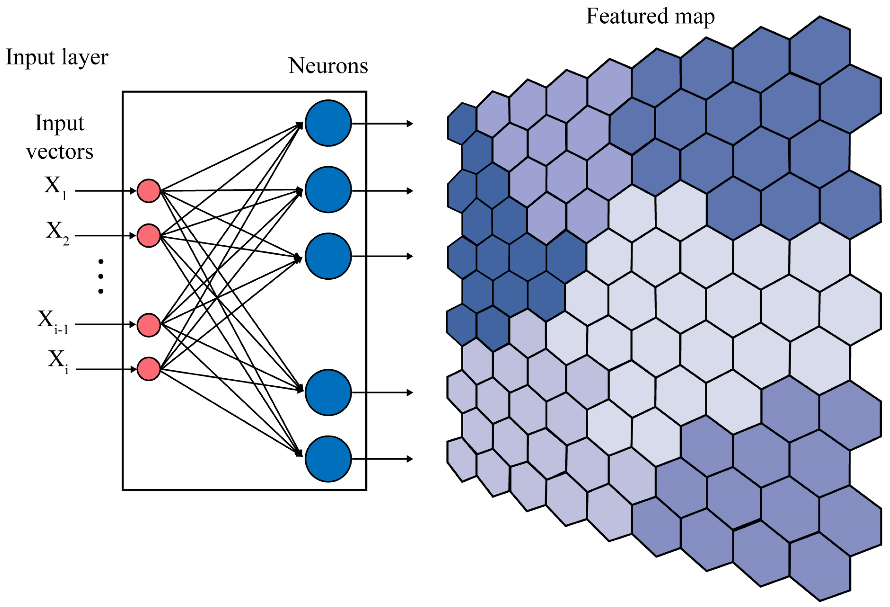
3.1. Self-Organizing Map

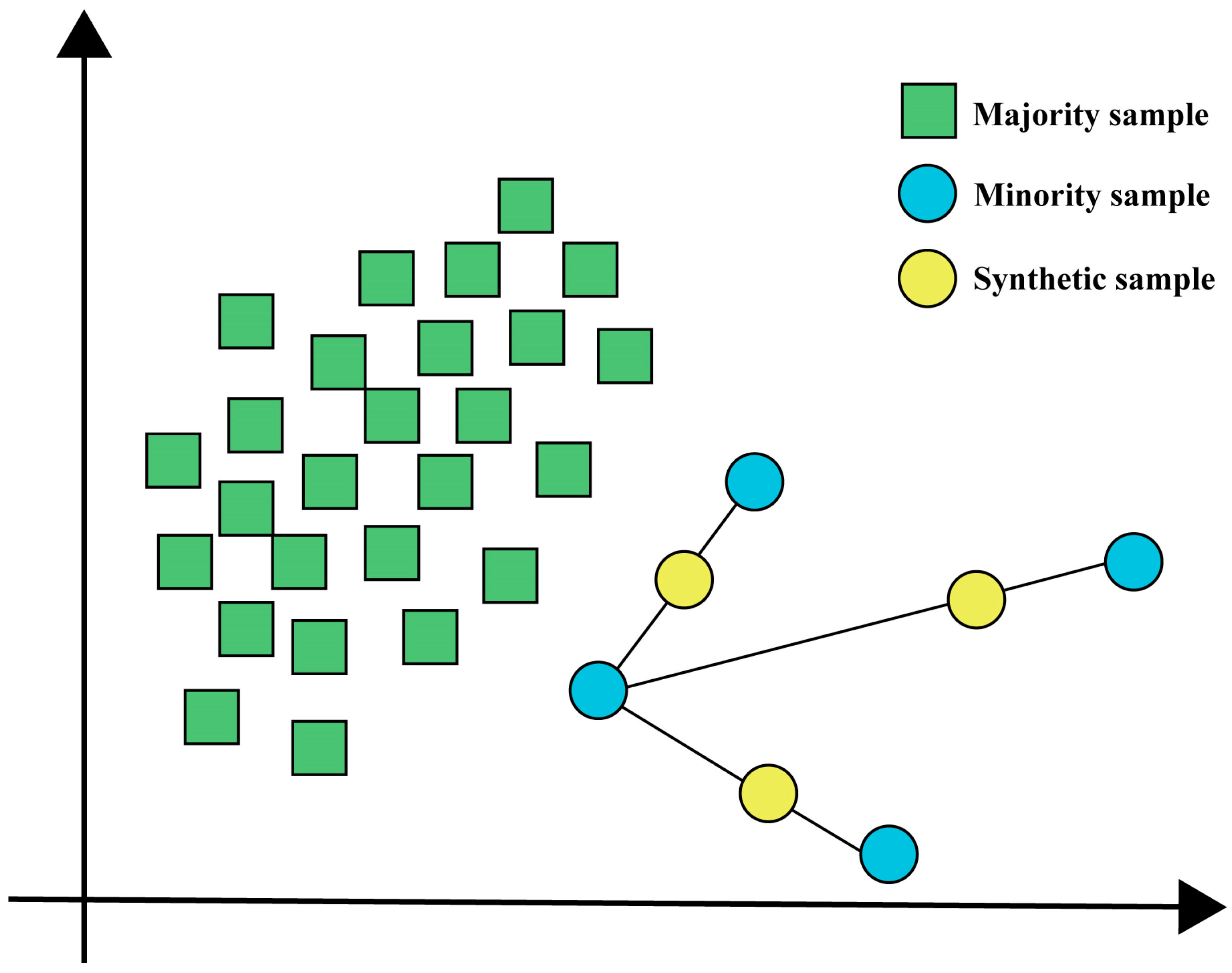
The SOM method is an artificial neural network approach that achieves clustering results through unsupervised learning [55]. This method is based on a competitive learning strategy that relies on the competition among neurons to gradually optimize the network, using neighborhood functions to maintain the topological structure of the input space, thereby facilitating self-organized training and clustering of similar neurons in a spatial distribution (Figure 7) [56]. In the SOM method, an input vector is assigned to the neuron unit with the most similar weight vector or the closest neuron, with appropriate metrics used to measure the distance between vectors. The general idea is that the weight vectors represented by each neuron are spatially correlated, thereby making the represented input vectors close, combined with a competitive strategy to identify the grouping forms of input data [57]. When a new input vector is introduced, the distance to each neuron’s weight vector is calculated, and the optimal neuron is selected as the best matching unit (BMU), with neighboring weights adjusted accordingly [58]. According to the following update equation, the magnitude of adjustment decreases with time and distance to the BMU.

$$W_{\nu }(t+1)=W_{\nu }(t)+\theta (v,t,d)\alpha (t)\left[D(i)-W_{\nu }(t)\right]$$

(1)

In the aforementioned equation, t represents the iteration number or round of the algorithm, D(i) denotes the input vector (where i is the sample size of the training dataset, ranging from 1 to n), θ(v,t,d) is the neighborhood function, which depends on the distance to the BMU, and α(t) is a monotonically decreasing learning coefficient.

Ultimately, the neurons or output nodes can be graphically visualized and associated with groups present in the input multi-dimensional space, where the color scale represents the distances between neurons stored in the U matrix.

This study is based on the theory of the K-means algorithm, utilizes Euclidean metrics to calculate distances between vectors, and employs the lowest Davies–Bouldin validity index to select the optimal clustering. To estimate the number of SOM nodes, a heuristic formula was used [59].

$$m=5\sqrt{n}$$

(2)

In the aforementioned equation, m represents the number of SOM nodes, and n denotes the number of samples in the input dataset.

3.2. SMOTE

It is well known that the data quality is optimal when the number of positive samples equals the number of negative samples in the training set. Therefore, when there is an imbalance between positive and negative samples, some strategies need to be adopted to alter the sample distribution, transforming the imbalanced samples into a relatively balanced state. Data resampling algorithms primarily include oversampling and undersampling [60]. The goal of oversampling is to increase the number of minority class samples to balance the class distribution in the dataset. As such, oversampling is more suitable for situations with small sample sizes compared to undersampling. The imbalance of the samples generated in oversampling and the variation in the oversampling rate can have a certain impact on the training results of the final machine learning model [61].

SMOTE (Synthetic Minority Over-sampling Technique) is an improved approach based on random oversampling algorithms [62]. Since random oversampling increases the number of minority class samples by simply duplicating samples, it can lead to overfitting of the model, meaning that the model learns overly specific information that is not generalizable. The basic idea of the SMOTE algorithm is to analyze the minority class samples and artificially add new samples to the dataset based on the minority class, as shown in Figure 8. This method creates several “synthetic” samples for each minority class sample by drawing line segments between k-nearest neighbor minority class samples. It then generates synthetic samples by computing the vector difference between the minority class feature vector and its nearest neighbor minority class feature vector. This difference is multiplied by a random number between 0 and 1 and added back to the minority class feature vector. This results in a random point being selected along the line segment between two minority class features, thereby increasing the number of minority class samples. Therefore, SMOTE expands the decision region of the minority class, making it more generalizable [63].

3.3. Support Vector Machine

SVM (Support Vector Machine) algorithms have been widely applied in binary classification tasks [64]. Initially developed for linear classification, they were later extended to non-linear classifiers and eventually adapted to regression tasks. The core concept of SVM is to construct an optimal margin classifier, where the complexity is a function of the number of support vectors, which means that only a small subset of the data that is crucial for constructing the classifier is required. Consequently, the SVM algorithm is particularly well suited for scenarios involving sparse samples and large-scale high-dimensional datasets [65].

For the classification of complex non-linear data, the use of a kernel function has been proposed to project the dataset into a higher-dimensional feature space, allowing for linear separation within this newly transformed space. Common kernel functions include linear, polynomial, radial basis function (RBF), and sigmoid kernels. By applying these kernel functions, SVM is able to transform non-linear problems in the original feature space into linearly separable problems in a higher-dimensional space, effectively increasing its flexibility and ability to handle a wide variety of complex relationships within data.

3.4. Random Forest

Random Forest (RF) is an extension of the Bagging algorithm; it is a typical ensemble method composed of multiple decision trees [66]. A decision tree is a tree-like structure where each internal node represents a test on an attribute, each branch represents an outcome of the test, and each leaf node represents a class label. In Random Forest, each decision tree is created through random sampling, where approximately two-thirds of the training samples are used to train the decision tree, while the remaining samples are used to quantify the accuracy of the prediction. Finally, by collecting the results from each decision tree, a simple averaging strategy is employed to predict the properties of new samples, according to the following formula:

$${\widehat{f}}_{rf}^K(x)={\displaystyle \frac{1}{K}}{\displaystyle \sum _{k=1}^K{f}_i}(x)$$

(3)

where $\widehat{y}$ represents the ensemble regression model, f_i(x) denotes the individual decision tree regression models, and K is the number of regression trees (i.e., N estimators).

In Random Forest (RF), each Decision Tree (DT) follows the same distribution, and the classification error is influenced by both the individual classification ability of the trees and their correlations. To increase the diversity between trees and reduce their correlations, sampling methods are typically employed to generate different subsets for training. However, since each tree uses only a portion of the training data, this may lead to suboptimal training performance. To address this issue, overlapping sampling techniques, such as bootstrap aggregation, are utilized. In this process, random sampling with replacement is performed on a dataset containing m samples to generate a training set of m samples. Approximately 36.79% of the samples are not selected; referred to as Out-of-Bag data, they do not contribute to the model training and can therefore be used for generalization validation. Random Forest effectively reduces the risk of overfitting through this method and enhances classification accuracy by aggregating multiple weak classifiers. This results in higher accuracy, smaller generalization error, and stronger overfitting resistance, outperforming other machine learning algorithms such as neural networks, regression trees, and Support Vector Machines [62]. Currently, Random Forest has been widely applied in various research fields of mineral resource exploration [33,67,68,69].

3.5. Positive–Unlabeled Learning

The objective of mineral exploration is to discover valuable ore bodies. Therefore, predicting new ore bodies in unknown areas based on the few ore bodies accumulated in geological data is highly significant. Positive–unlabeled learning (PUL) is a one-class classification algorithm in which the sample data types consist only of positive samples (P) and unlabeled samples (U). By analyzing the characteristics of known positive samples, the algorithm identifies the most probable samples in U that share the same data features as potential positive samples. Through self-sampling with replacement, an equal number of unlabeled samples can be selected for training alongside the positive samples. In mineral exploration, a small number of ore bodies can serve as positive samples, while a vast amount of non-ore body data can be used as unlabeled samples. The PUL algorithm offers significant advantages in mineral prediction during quantitative evaluation [37,67]. In this study, an improved positive–unlabeled learning (PUL) algorithm called Bagging-based positive–unlabeled learning (BPUL) is adopted, which incorporates the concept of Bagging. By employing the Bagging method, we repeatedly and randomly selected equal amounts of unlabeled samples to serve as negative samples for constructing training sets. This approach allowed us to train a series of base learners. We then made predictions on the unlabeled samples that were not selected, recording and calculating their average scores to obtain the final optimal training model.

The predefined number of iterations is set to N. Upon completion of the iterative process, all scores for each sample are recorded. The final score S(x) for each sample in U is calculated by computing the average of its scores; thus,

$$S(x)={\displaystyle \frac{{{\displaystyle \sum }}_{i=1}^{N}f(x,i)}{N}}=E(f(x,i)),i=1,2,\cdots N$$

(4)

The comparison of errors between the base learners and the BPUL algorithm can be achieved through expectations. For the labeled samples (Y) and each base learner f(x,i), the inequality E(Z²) ≥ (E(Z))² holds. Therefore,

$$E({(Y-f(x,i))}^2)=Y^2-2YE(f(x,i))+E(f^2(x,i))\ge {(Y-S(x))}^2$$

(5)

From the above equation, it is evident that the BPUL algorithm exhibits smaller errors compared to the base learners. By averaging the outputs of these base learners, the impact of unreliably selected negative samples is mitigated. Furthermore, various data-driven algorithms or models can be employed as base learners within the BPUL framework.

3.6. Bayesian Optimization

Selecting appropriate hyperparameters is crucial for ensuring the performance of the trained model. Common parameter optimization methods include grid search, random search, and Bayesian optimization [70]. Grid search performs poorly when the number of parameters is large, consuming excessive computational power and sometimes even failing to find the optimal solution. Random search selects parameters randomly and lacks intelligence in parameter selection. Moreover, neither grid search nor random search exploits the correlations between different hyperparameter combinations [71]. Currently, Bayesian optimization is becoming increasingly popular as an intelligent hyperparameter optimization algorithm and is being more widely applied [68]. Bayesian optimization is typically used in conjunction with classifiers such as logistic regression, SVM, Random Forests, XGBoost, and neural networks. Sequential Model-Based Optimization (SMBO) is the core procedure of Bayesian optimization algorithms [67]. The procedure includes two key functions: the surrogate function and the acquisition function. SMBO first establishes an initial surrogate model M₀ and an experimental set H. The surrogate model M₀ serves to link the hyperparameter settings x with the loss function F, while H records each set of hyperparameters along with their corresponding loss values and is used to update the surrogate model [72].

Sequential Model-Based Optimization (SMBO) then obtains the optimal hyperparameters through the following iterative process:

• Search and obtain the locally optimal hyperparameters x* on the current surrogate model M_t−1 using the acquisition function.
• Calculate the actual loss value y of x*.
• Update x* and y into the experimental set H.
• Retrain the surrogate model using the updated H to obtain a new surrogate model M_t.

In this study, we used the Tree-structured Parzen Estimator (TPE) as the acquisition function and Expected Improvement (EI) as the surrogate function. Multiple experiments were conducted in total, with each iteration repeated several times to minimize the loss function of the surrogate function, thereby improving the overall performance of the model. Upon completion of the iterations, the global optimal hyperparameters x^∗ corresponding to the minimal loss value y were obtained.

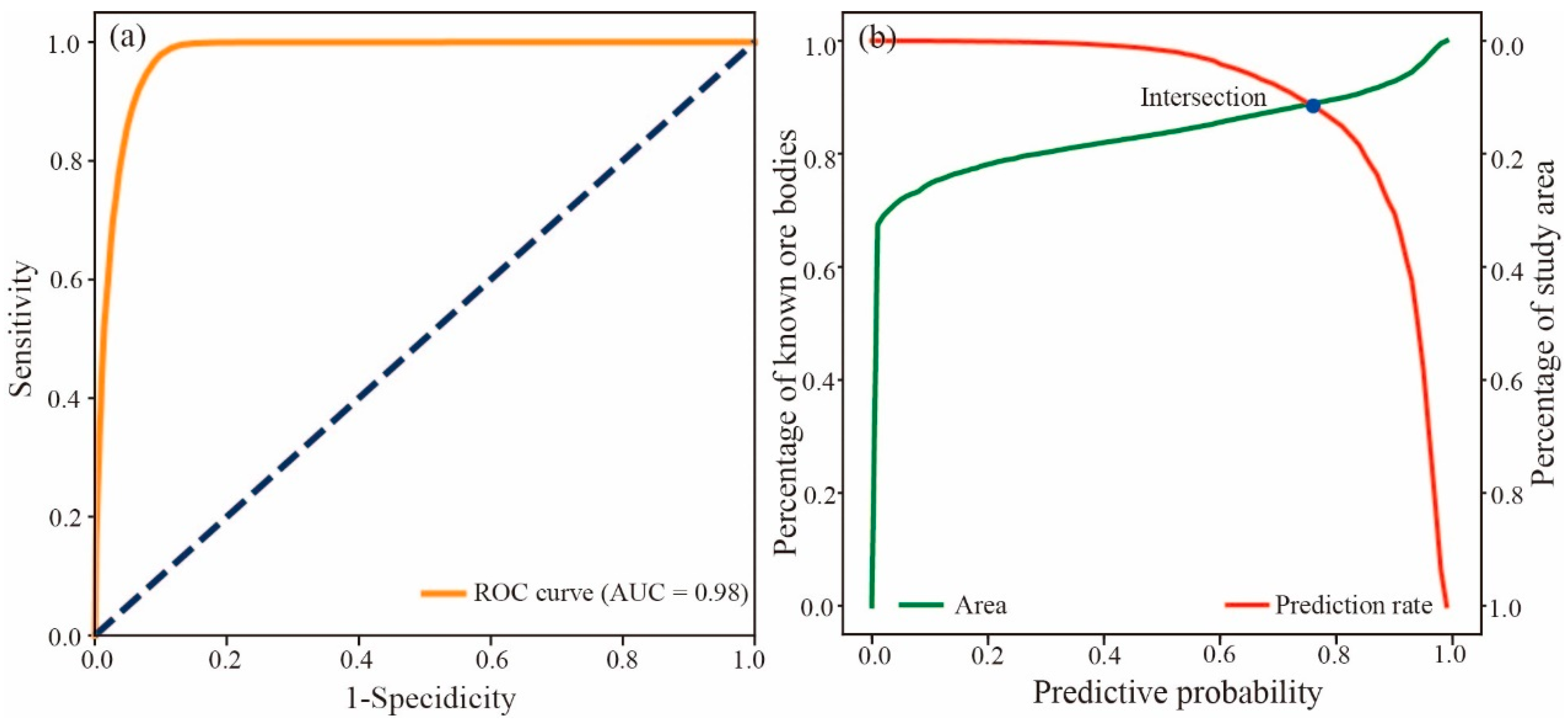
3.7. Model Evaluation Method

To evaluate the predictive performance of the MPM training model, traditional evaluation metrics such as recall, precision, and F1 score [73] are used; these metrics are composed of true positives (TPs), true negatives (TNs), false positives (FPs), and false negatives (FNs). A higher F1 score indicates better performance. The formulas for recall, precision, and F1 score are as follows:

$$recall={\displaystyle \frac{\mathit{True}\mathit{Positive}}{\mathit{True}\mathit{Positive}+\mathit{False}\mathit{Negative}}}$$

(6)

$$precision={\displaystyle \frac{\mathit{True}\mathit{Positive}}{\mathit{True}\mathit{Positive}+\mathit{False}\mathit{Positive}}}$$

(7)

$$F1\mathrm{s}\mathrm{c}\mathrm{o}\mathrm{r}\mathrm{e}=2\cdot {\displaystyle \frac{precision\times recall}{precision+recall}}$$

(8)

Receiver Operating Characteristic (ROC) curves and the Area Under the Curve (AUC) are also commonly used to evaluate the performance of predictive models in Mineral Prospectivity Mapping (MPM) [74]. The ROC curve plots the false positive rate on the X-axis and the true positive rate on the Y-axis to describe the model’s performance. The AUC value ranges between 0 and 1, with higher values indicating better model performance [75].

In addition, Prediction–Area (P-A) plots are widely used to evaluate model performance This plot features two curves representing the prediction rate curve and the occupied area curve—that is, the ratio of the known mineralized area within the target area to the total known mineralized area, and the ratio of the target area to the total area, respectively [76]. These curves illustrate the relationships among the study area, the target area, and the known mineral deposits. As the prediction probability increases from 0 to 1, the two curves intersect at a point, indicating that the maximum number of known mineral deposits is concentrated within the smallest target area. The higher the Y-value at the intersection point, the better the model’s performance [77]. Therefore, the higher the intersection point on the P-A plot, the better the predictive model performs, enabling the discovery of as many known mineral deposits as possible within a limited target area and facilitating the delineation of new mineralization targets.

4. Results and Discussion

4.1. Sample Testing and Analysis

In this study, a total of 395 samples were subjected to XRF elemental grade determination. The major elements are primarily Si and Fe (Figure 9a), while the trace elements are mainly Rb and Sr (Figure 9b). Non-ore samples with Fe content below 20% were excluded in subsequent analyses. Elemental geochemical characteristics were then studied for 218 ore samples, focusing on their content characteristics, cluster analysis, and principal component analysis results. After excluding unidentified rare earth elements, the major elements analyzed include Si, Fe, Al, Mg, Ca, K, Ti, Mn, S, and Co, while the trace elements analyzed include Sr, Rb, Cr, Zr, V, Zn, Ni, Cu, Y, Pb, Mo, Th, and Nb. Geochemical data are typical compositional data. Before data analysis, appropriate transformations such as normalization and centered log-ratio (CLR) transformation are required to ensure that the data follow a normal distribution and to eliminate the influence of the “closure effect” [78,79].

The composition plane of the elemental contents of the samples is presented in Figure 10. A self-organizing map (SOM) of the sample elements was constructed using a color gradient, where each color corresponds to a different value of a given variable, and each hexagon represents a neuron in the component plane. Elements with similar color patterns exhibit positive correlations, while those with distinct colors exhibit negative correlations. As illustrated in Figure 10b,c, when the number of clusters is set to 2, the Davies–Bouldin (DB) index reaches its minimum value of 0.632, indicating the optimal clustering solution.

Based on the self-organizing map of individual sample elements shown in Figure 10a, the sample elements can be divided into two interpretable clusters. In the first cluster, elements such as Mg, Al, Si, S, K, Ca, Mn, and Fe exhibit a pattern where the neuron concentration in the lower-left region is higher, gradually decreasing towards the upper-right corner. However, elements like Ti and Co show a similar pattern to Fe, with a higher neuron concentration in the lower-left region and a gradual decrease towards the upper-right corner. Elements like Zn and Sr, on the other hand, only show small regions of high neuron concentration in the lower-left corner or small regions of lower concentration in the upper-right corner. In contrast, elements such as V, Cr, Ni, Cu, Y, Zr, Nb, Pb, and Mo show an opposite distribution, where concentration increases gradually from left to right, forming a horizontal gradient. This pattern suggests that there is a strong positive correlation among Mg, Al, Si, S, K, Ca, Mn, and Fe, a general positive correlation between Ti, Co, and Fe, a weaker positive correlation between Zn, Sr, and Fe, and a negative correlation between these elements and V, Cr, Ni, Cu, Y, Zr, Nb, Mo, and Pb. In the second cluster, the elements Rb and Th both exhibit lower neuron concentrations in the lower-middle region, with higher neuron concentrations surrounding them. This observation confirms the positive correlation between Rb and Th in this area, with almost no correlation to Fe.

Currently, infrared spectroscopy technology can be divided into shortwave infrared (SWIR) and thermal infrared (TIR) based on spectral ranges. With the use of portable spectrometers, data from different spectral ranges have been widely analyzed for mineral exploration to identify and characterize alteration minerals in different regions [80,81]. In the shortwave infrared (SWIR) range, various diagnostic absorption features based on different functional groups such as H₂O, Mg-OH, Fe-OH, Al-OH, CO₃²⁻, SO₄²⁻, and NH⁴⁺ can effectively identify hydroxyl, amine, carbonate, and sulfate minerals in geological samples. Additionally, scalar measurements of common absorption features in the shortwave infrared range, such as absorption feature position (Pos) and depth (Dep), can be used to characterize their metallogenic environment, chemical properties, and crystallinity. On the other hand, mid-infrared thermal radiation detects molecular vibration fundamentals, which can effectively identify non-hydroxyl silicates (e.g., quartz, feldspar, garnet), carbonates, and sulfates [53].

After spectral data from the SWIR and TIR intervals of the samples were obtained, mineral identification was conducted using TSG. The results (Figure 11) indicate that the main alteration minerals in the region are from the chlorite group (chlorite-Fe, chlorite-Mg, chlorite), mica group (muscovite, biotite, mica), carbonate group (siderite, dolomite, calcite), as well as montmorillonite, amphibole, quartz, and feldspar (sodium feldspar, microcline) (Figure 9a,b). Since the samples were generally collected from the ore body and its vicinity, the analysis results provide certain indications for the distribution of the ore body. After the combination of the geochemical element analysis results, which show a strong positive correlation between elements such as Mg, Al, Si, S, K, Ca, Mn, and Fe, it can be inferred that the widespread chloritization (with chlorite mineral formula (Mg,Fe,Al)₆(Si,Al)₄O₁₀(OH)₈) and carbonation (mainly dolomite with mineral formula CaMg(CO₃)₂) alteration features in this region are closely related to metallogenic processes. These findings provide effective theoretical evidence for alteration factors in subsequent 3D metallogenic predictions. Elements such as Mg, Al, Si, Ca, and others that show a strong positive correlation with Fe can serve as indicator elements to guide the next stage of deep mineral exploration in this area.

4.2. Intelligent Detection of UAV Images

After the process of radiometric calibration, a quantitative relationship was established between the digital quantization values of the unmanned aerial vehicle (UAV) remote sensing imagery and the corresponding radiance values of the field of view. Additionally, since these images were captured by a lightweight UAV at an approximate altitude of 80 m above the ground under clear weather conditions, they are almost unaffected by atmospheric influences. The multi-temporal UAV multispectral images of the mining area are illustrated in Figure 3.

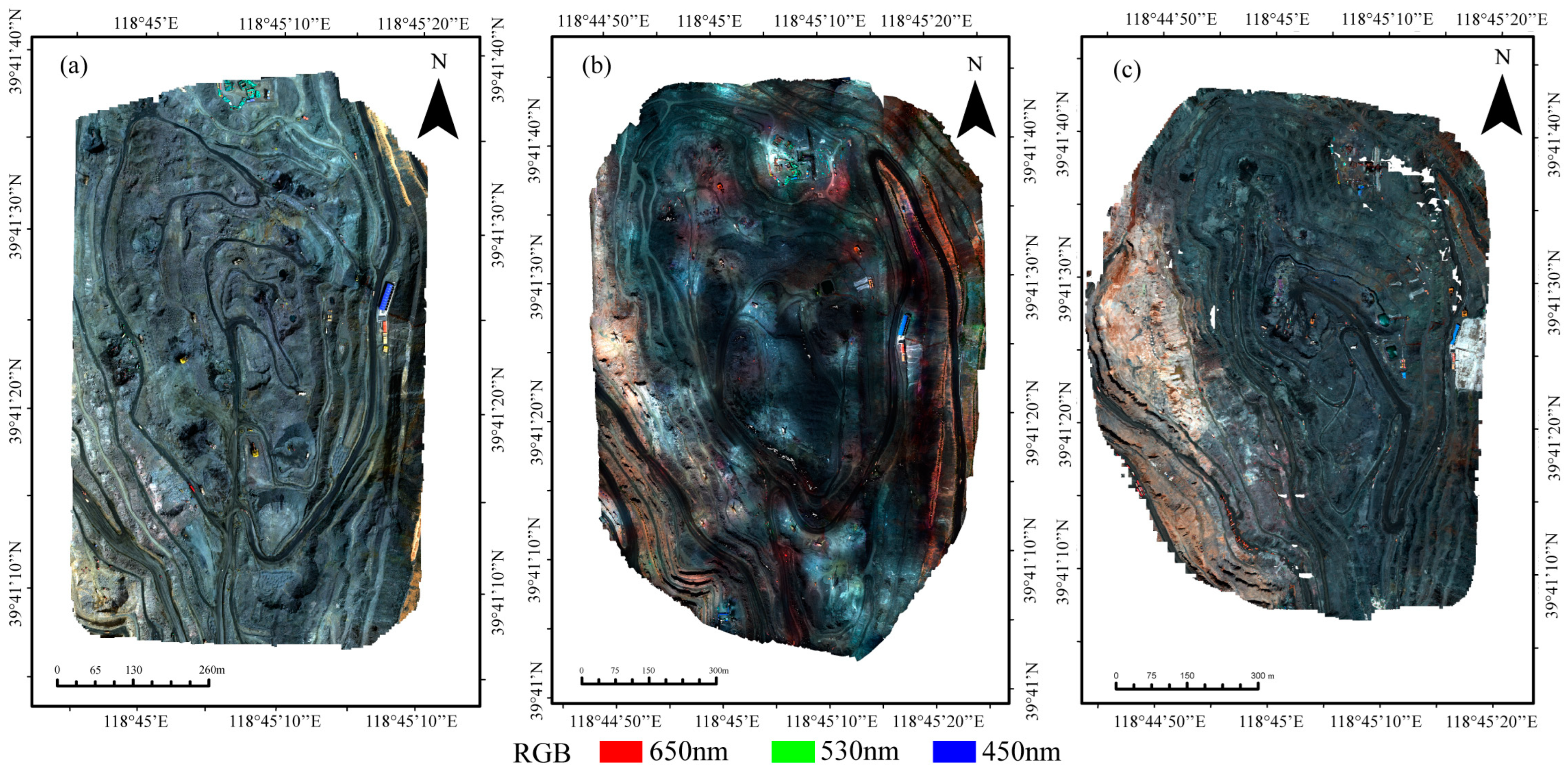
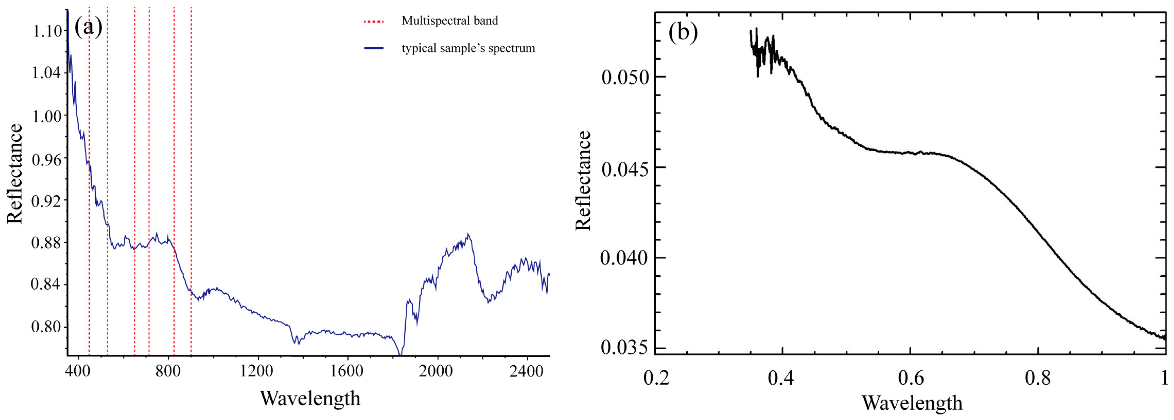
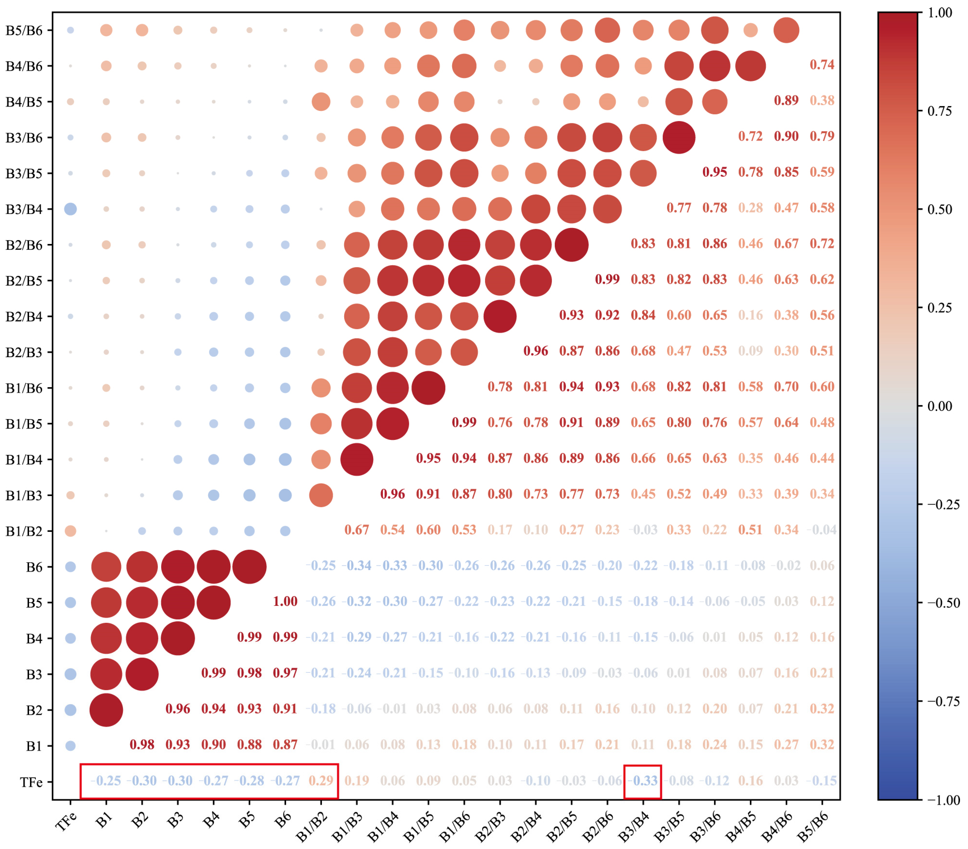
4.2.1. Band Preference

In examining the spectral characteristics of typical magnetite ores in the region, including the typical sample spectra collected and those from the USGS database (as shown in Figure 12), it is observed that the mineral exhibits a nearly linear decline from 400 nm to 1000 nm. In the typical magnetite spectral curve from the Yanshan Iron Ore Mine, there are small absorption peaks only at 650–720 nm and 900 nm. Therefore, this study introduces a new index—the band ratio index—based on the original spectral bands. This index reflects the relative spectral transformation of magnetite and can reveal its dynamic spectral properties. By calculating the Spearman correlation coefficient between the spectral bands and iron grade, the relationship between the spectral band information from remote sensing images and the actual iron grade measurements can be explored, allowing for the identification of bands and band ratio indices that have a high correlation with iron grade inversion (i.e., intelligent identification of magnetite).

Given n samples, the original spectral data were first standardized and then transformed into rank data. The Spearman correlation coefficient (ρ) was subsequently calculated using the following equation to assess the relationships:

$$\rho ={\displaystyle \frac{{\displaystyle \sum _i(x_i-\overline{x})}(y_i-\overline{y})}{\sqrt{{\displaystyle \sum _i{(x_i-\overline{x})}^2}{\displaystyle \sum _i{(y_i-\overline{y})}^2}}}}$$

(9)

Utilizing the results of the Spearman correlation coefficient calculations (as shown in Figure 13), eight spectral bands and band indices with significant relationships with iron grades at a level above 0.2 were selected. These include six individual bands, as well as the ratios of 450 nm to 530 nm and 650 nm to 720 nm, which will provide features for the subsequent intelligent recognition of magnetite.

4.2.2. Magnetite Identification

This study employs the Random Forest and Support Vector Machine (SVM) methods to predict ore grades in remote sensing images of the mining area, constructing a model that links sample spectral features with ore grades for the intelligent identification of magnetite (iron grade). A total of 329 samples collected during the second phase were selected as the training and prediction set for the machine learning algorithms. Ore with an iron grade greater than 20% in the Yanshan Iron Ore Mine is labeled as effective ore, while the remaining is considered waste rock. In fact, considering that grade is a continuous variable rather than a discrete one, the 20% grade threshold is an arbitrary cutoff. Therefore, ores with grades around 20% show little difference, and it is challenging to effectively distinguish such ores using spectral features. To enhance the representativeness of the training samples, this study randomly samples 30 times. In each iteration, two-thirds of the samples with scores lower than 10% are randomly selected as negative samples, while all samples with scores higher than 30% are used as positive samples. However, since there are only 29 positive samples, and two-thirds of the negative samples total 94, to maintain the balance between positive and negative samples, the SMOTE algorithm [62] is used to generate artificially synthesized negative samples for training. These positive, negative, and synthetic samples are then merged to form the training set for the model. After each random sampling, the training results are statistically analyzed, and the optimal result is selected as the prediction model for the intelligent identification of magnetite. Furthermore, Bayesian optimization is used to fine-tune the hyperparameters during each model training process. The search space for the hyperparameters of the optimal Random Forest and Support Vector Machine models and the best parameters selected through Bayesian optimization are shown in

Table 4. Hyperparameter adjustments of SVM and RF.

Method	Parameters	Skopt Best Parameter	Search Range
SVM	C	0.79	[1 × 10−6, 1 × 106] (log-uniform)
	kernel	rbf	[linear, rbf. Sigmoid]
RF	n_estimators	500	[10, 500]
	max_depth	50	[5, 50]
	min_samples_split	2	[2, 20]
	min_samples_leaf	1	[1, 20]
	criterion	gini	[gini, entropy]

.

Based on the evaluation results of the training models after 30 rounds of random sampling for both Random Forest (RF) and Support Vector Machine (SVM), the AUC value of SVM12 is notably higher than that of the other SVM models (Figure 14a). In contrast, the AUC values of the RF models are primarily distributed within the range of 0.836 to 0.852, with RF23 showing a slightly higher AUC than the other RF models (Figure 14c). The overall stability of the Random Forest method is superior to that of the Support Vector Machine. A comparison of the confusion matrix results for SVM12 and RF23 (Figure 14b,d), as well as the evaluation metrics, including accuracy, recall, F1 score, and AUC, reveals that while RF23 and SVM12 are similar in accuracy, RF23 outperforms SVM12 in all other metrics. Specifically, RF23 shows significant improvements in recall and AUC (

Table 5. Optimal model accuracy, recall, and F1 score of SVM12 and RF23.

Predictive Models	Recall	Precision	F1 Score
SVM12	0.75	0.78	0.76
RF23	0.80	0.79	0.79

; Figure 15). These results demonstrate that Random Forest provides superior performance in magnetite recognition compared to Support Vector Machine.

Subsequently, the RF23 model was applied to predict the entire region of a multispectral image, with the results shown in Figure 16. The prediction results indicate a clear boundary between the high and low mineralization areas. In Figure 16a, regions 1 and 2 represent high mineralization areas, while regions 3 and 4 correspond to low mineralization areas. The distribution of samples aligns well with the predicted two-dimensional magnetite mineralization levels, further confirming the reliability of this method for intelligent recognition of two-dimensional magnetite. At the same time, we zoomed in on the magnetite identification results in the local ore stockpile area, allowing for a clearer and more intuitive view of the distinct boundaries between rocks and minerals. From the comparison results of Figure 16b,c, it can be observed that the red-boxed area on the right side of Figure 16b represents the rock powder stockpile area. The high-grade region without white cloth coverage and the low-grade region covered with white cloth in the stockpile are both clearly highlighted. The red-boxed area on the left side of Figure 16b represents the face of the open-pit excavation area, where the boundary between rock and ore cannot be effectively distinguished in the visible light angle of the DOM image (Figure 16c). However, in the multispectral image’s intelligent interpretation and recognition results, the rock–ore boundary is very clear and can effectively guide real-time mining operations in the area.

The raster image of intelligent recognition of magnetite in 2D form is converted into point data in ArcGIS_Pro 3.4. Then, the surface elevation information obtained during LiDAR imaging is appended to it, forming a three-dimensional surface magnetite intelligent recognition result with elevation attributes, as shown in Figure 17. The recognition model of this technology not only displays the magnetite prediction results for the entire mining area, as shown in Figure 17, where the overall iron grade of the mining area is relatively low, and the iron grade in the central and western mining areas is slightly higher, but it can also significantly compress the task completion time by hours through the instantaneous availability of data. This enables dynamic risk control and resource optimization, such as real-time mining guidance and monitoring of slope stability, reducing the cost and risk of traditional manual exploration and improving production efficiency and safety. Additionally, this technology can not only quickly interpret and identify mining areas but also detect the diffusion of heavy metal pollution (such as arsenic and mercury) in tailings using spectral features and assess the ecological restoration effect using NDVI.

4.3. Three-Dimensional Metallogenic Prediction

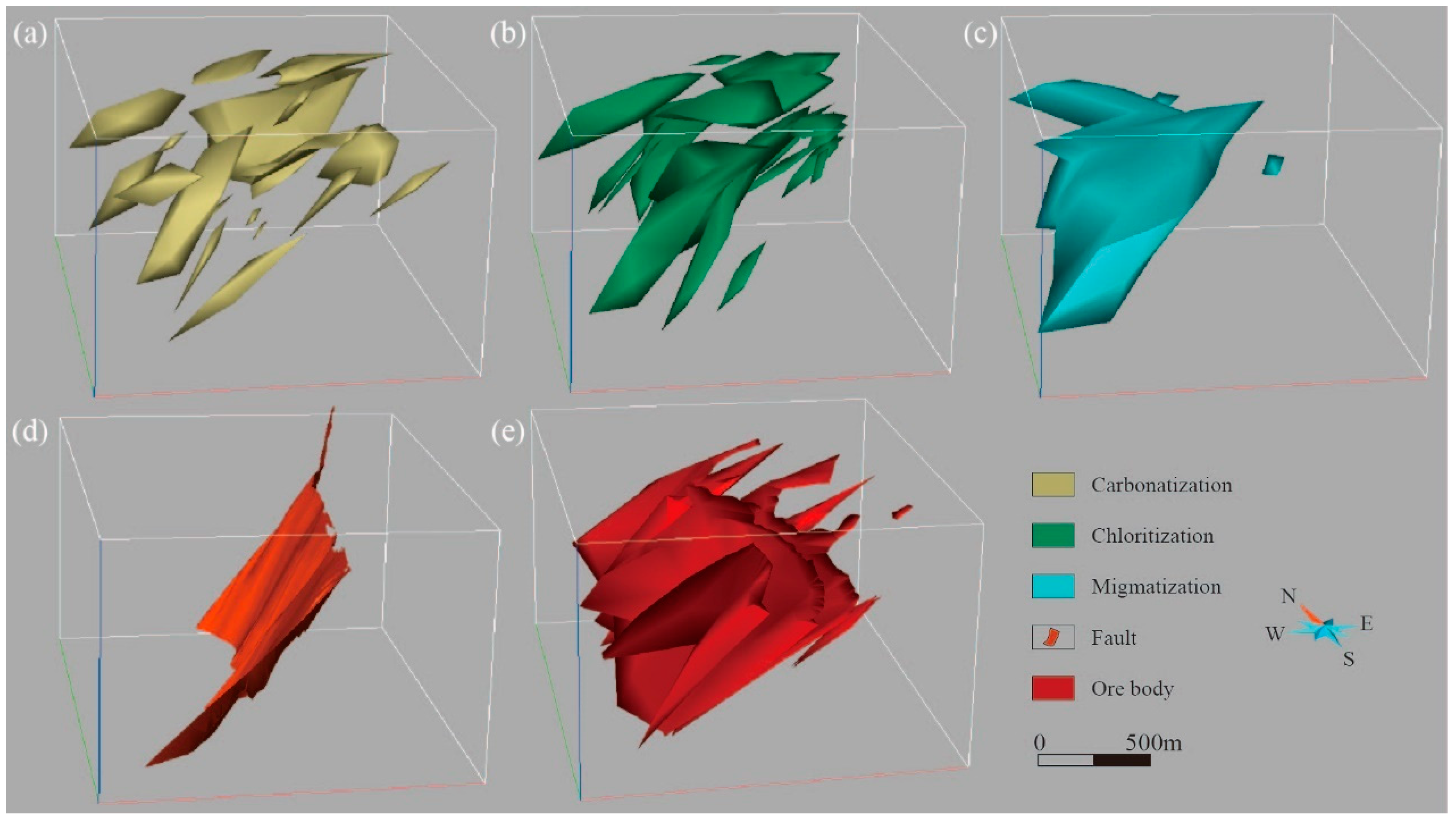
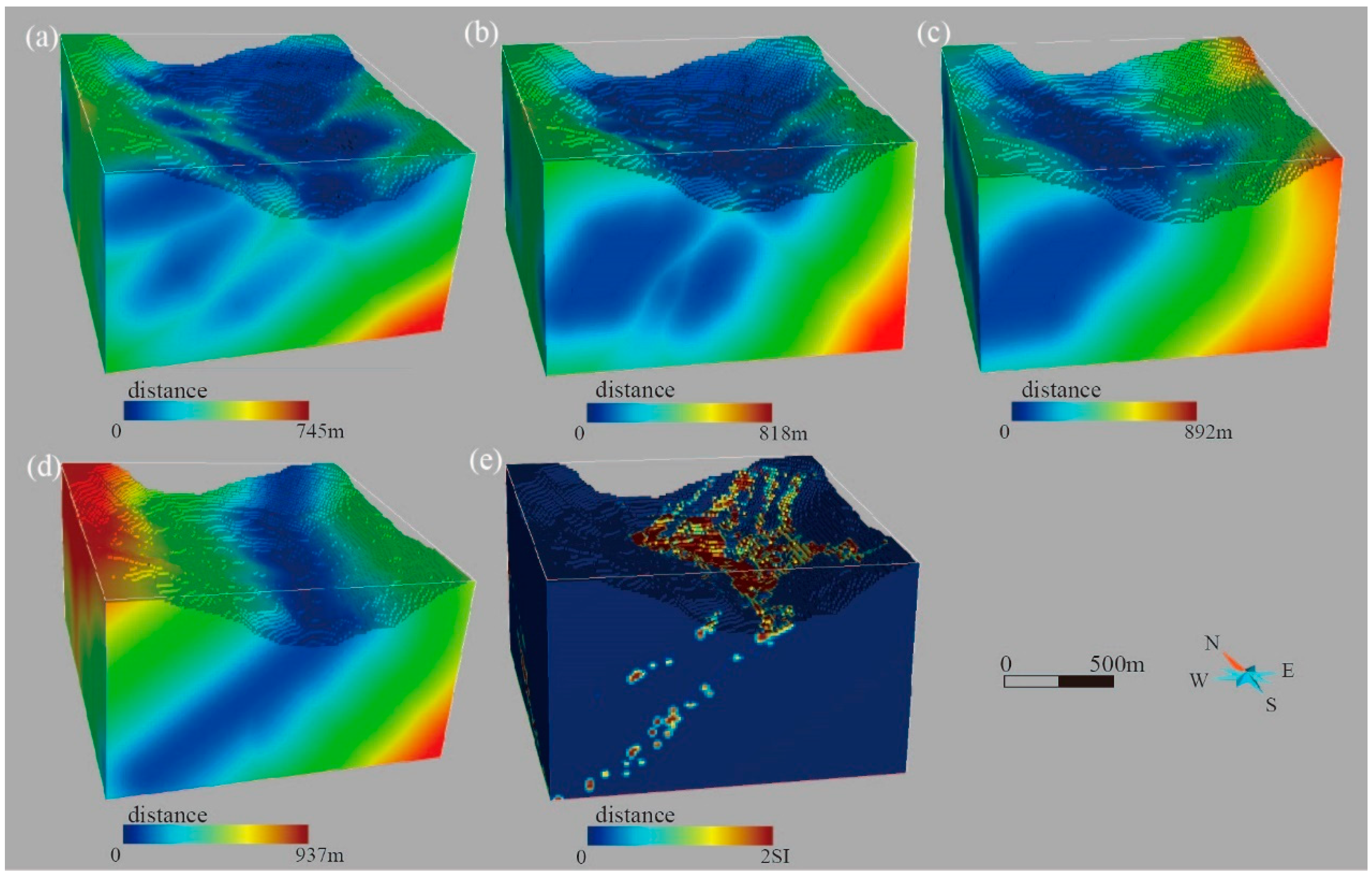
4.3.1. Three-Dimensional Exploration Criteria

Based on the concept of a mineral system, this study examines the critical processes related to the Yanshan iron ore deposit—transport, traps, and deposition in terms of rock, faults, and hydrothermal alteration [82,83]. The expressions of each of these processes in relevant geoscience spatial data are deemed mappable criteria for exploration targeting. The objective of this analysis is to identify geological ore-controlling factors closely associated with mineralization, establish an exploration model, and provide a theoretical foundation for the exploration of highly mineralized areas within the mining region using multi-source and multi-dimensional data [84]. The metallogenic elements of Yanshan Iron ore are shown in

Table 6. Exploration targets of the Yanshan iron deposit.

Expression of Critical Processes	GIS-Based Targeting Criteria
The magnetic anomaly of the ore body is higher than that of the surrounding rock, and the magnetic anomaly significantly indicates the presence of rich ore.	Aeromagnetic anomaly
The fold structures provide migration pathways for hydrothermal activity, facilitating the formation of rich ore deposits.	Proximity to Sijiaying compound syncline; proximity to migmatization
Hydrothermal alteration is pronounced in areas near rich ore bodies.	Proximity to chloritization and carbonatization

.

The folds and faults are predominantly developed within the metamorphic rock series and are well defined, significantly influencing the localization of ore deposits, particularly at fold hinges and fault intersections. The closely developed folds and fault structures serve as critical external factors in the hydrothermal alteration of low-grade ore bodies, facilitating migration pathways for hydrothermal activity and creating spaces for the enrichment of ore-forming components [42]. Among these factors, fault structures demonstrate the most significant ore-controlling effects. The intersections of various fault sets, along with faults that transect low-grade ore bodies, facilitate the transport of hydrothermal fluids, induce alterations in the ores, and activate iron through these fluids, ultimately contributing to the formation of rich iron deposits. Consequently, the fault structures, folds, and other geological features in this area establish favorable conditions for the development of high-grade iron ore deposits [46].

Research indicates that migmatization and hydrothermal alteration are key factors in the enrichment of the Yanshan iron deposit. The crystalline basement in the mining area has undergone a high degree of metamorphism, transitioning from granulite-facies to greenschist-facies metamorphism, accompanied by intense and widespread migmatization. Large areas of gneissic migmatite are present at the top of the ore body. Simultaneously, strong hydrothermal alteration is observed around the ore body, with common alteration types including chloritization, carbonatization, biotitization, and muscovitization. The widespread development of interlayer faults and fracture zones further facilitates hydrothermal activity. Therefore, the intersections of migmatization, hydrothermal alteration, and fault structures represent critical zones for the concentration of iron-rich ore bodies [85].

In addition to the aforementioned geological factors, the primary iron mineral in this region is magnetite, which possesses a high magnetization rate and exhibits a distinct magnetic contrast with the surrounding rocks, including metamorphic rocks, migmatites, gneisses, diorites, and basalts. The magnetic anomalies associated with magnetite are important indicators for mineral exploration in this area. Exploration results from the Second Geological Team of the Hebei Provincial Bureau of Geology and Mineral Resources (2010) [44] detected positive magnetic anomalies ranging from 9000 to 12,000 nT at the outcrop locations of the ore bodies in the Yanshan mining area, confirming that magnetic survey data are reliable indicators for the distribution of ore bodies in this area [43].

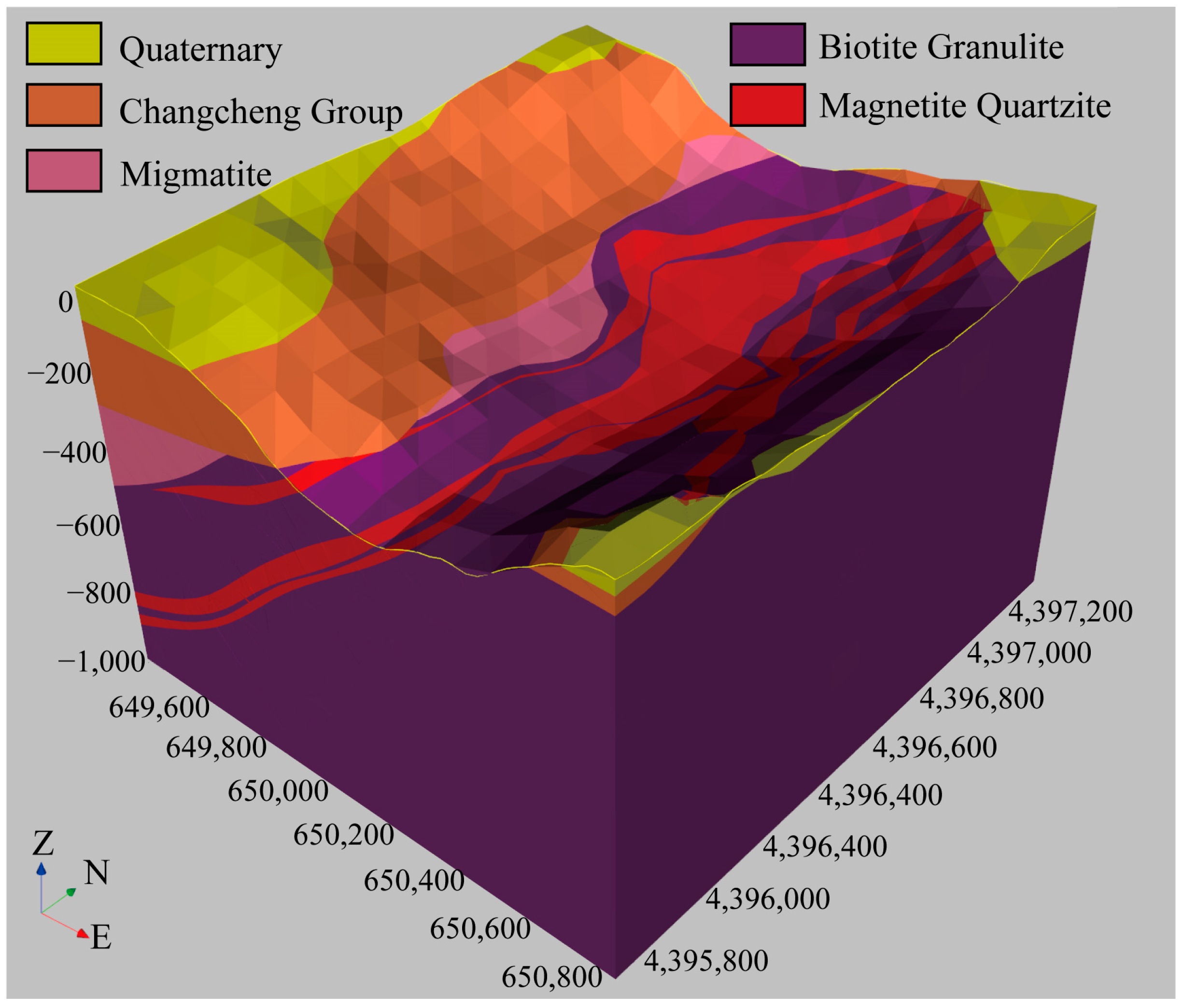
4.3.2. Three-Dimensional Geological-Geophysical Modeling

The spatial information of different geological interfaces, including faults, lithology, alteration, etc., was extracted based on existing geological data (such as planar geological maps, borehole data, cross-sections, and intermediate plane data). Explicit modeling was performed using platforms like Micromine and GOCAD, and the geological interfaces were constructed through human–computer interaction. The closure function of the 3D modeling software was used to ensure the closure of geological interfaces. Three-dimensional geological models, including carbonatization, chloritization, migmatization, faults, ore bodies, and others, were constructed (Figure 18). Geological structure, alteration, and ore bodies are all controlled by the north–south trending fault, with a westward dip of 40–50°, forming a layered arrangement. As shown in Figure 18, metasomatism is primarily distributed in the upper part of the ore body, while carbonate alteration, chloritization, and other alterations are widely distributed in the ore body and its surrounding areas. The F4 fault has an NE-SW strike, a dip direction of 135°, and a nearly 45° dip angle, crossing through the entire ore body.

In this study, 11 exploration line cross-sectional profiles of the mining area in Geomodeller were utilized to delineate the deep geological contact zones and structures. Using the potential field geostatistical method, the interfaces between known geological bodies were interpolated and converted into discrete points, which were then used to divide the adjacent units in three-dimensional space. These cells were merged to construct a three-dimensional voxel model of the geological body. The model was compared with field data to identify and correct any defects, ensuring its consistency with geological principles. Ultimately, a reliable three-dimensional stratigraphic model of the Yanshan Iron Mine was generated (Figure 19). Based on Figure 1c and Figure 19, the Quaternary strata and the Mesoproterozoic Changcheng Group were identified as the sedimentary cover, unconformably overlying the New Archaean Xintaizi Group, consisting of migmatite, biotite-bearing granulite, and magnetite quartzite. In the deeper mining area, the magnetite quartzite (ore body) and biotite-bearing granulite (host rock) were distributed in an interbedded manner with relatively thin interlayer spacing. The magnetic reference values for the geological bodies within the model were then assigned (Table 2) to calculate the theoretical magnetic field. Finally, by integrating the ground and airborne magnetic survey data of the mining area (Figure 4), iterative magnetic forward modeling was conducted to refine the model boundaries and physical property amplitudes. The final three-dimensional magnetic susceptibility model of the mining area (Figure 20e) was constructed by controlling the magnetic field residuals within an acceptable precision range.

The study area covered by the 3D model extended over 1430 m in the E–W direction, 1570 m in the N–S direction, and 1040 m vertically, from 50 m above sea level to −990 m below sea level. The deposit-scale geological model of the study area was constructed using SKUA-GOCAD, and it was composed of 2,120,395 3D-grid voxels with a size of 10 × 10 × 10 m. The 3D block model will be used for the subsequent generation of 3D predictor maps and prospectivity maps.

Furthermore, through Euclidean distance analysis, this study generated the distances of carbonatization, chloritization, migmatization, and faults (Figure 20). These models serve as evidence layers for subsequent mineralization prospectivity analysis at the deposit scale. Furthermore, the constructed 3D ore body model serves as positive samples for subsequent three-dimensional mineralization predictions.

4.3.3. Three-Dimensional Prospectivity Mapping Based on BPUL

In this study, 183,390 voxels from positive samples and 2,540,043 voxels from unlabeled samples were input into the PU learning model. The Bagging-based PUL algorithm optimizes the hyperparameters of its base learner (Random Forest) through Bayesian hyperparameter optimization in each iteration. The hyperparameter search space and optimal hyperparameter selection for Bayesian optimization are shown in

Table 7. Hyperparameter adjustments of BPUL.

Method	Parameters	Skopt Best Parameter	Search Range
RF	n_estimators	35	[1, 100]
	max_depth	481	[1, 500]
	min_samples_split	12	[1, 20]

. After 10 iterations, the BPUL model achieved a prediction accuracy of 0.98, a recall rate of 0.98, and an F1 score of 0.99, demonstrating high predictive performance. The optimal model had n_estimators set to 35, max_depth set to 481, and min_samples_split set to 12 (

Table 8. Optimal model accuracy, recall, and F1 score of BPUL.

Predictive Model	Recall	Precision	F1 Score
BPUL	0.98	0.98	0.99

).

The performance of the BPUL model was evaluated using both ROC analysis and the P-V plot. The AUC value of 0.98 indicates that the BPUL model performs well in predicting the potential areas of the Yanshan ore deposit (Figure 21a). The intersection point in the P-V plot shows that, based on the BPUL model, 90% of the known ore voxels are delineated within 10% of the study area (Figure 21b). This identifies the high-prospect region as a potential target area for future mineral exploration. By selecting the optimal threshold from the P-V plot intersection, the high-prospect area is separated from the low-prospect background area. As shown in Figure 22a, the high-prospect area (with a probability > 0.75) has a strong correlation with the known ore bodies and exhibits a consistent spatial distribution with the fault zones, aligning with the geological features of the region. Figure 22b is the result map of the mineralization probability, further determined based on the high mineralization region shown in Figure 22a. According to the high mineralization belt depicted in Figure 22a, two key target areas were identified, located in the northwest and deep extension zones of the mining area, which are similar to the current exploration potential location of the Yanshan Iron Mine [46]. In the northwest of the mining area, the high mineralization belt predicted by the BPU model is significantly larger than the known ore body and extends outward. Figure 22b indicates that there is still a high mineralization belt along the 45° dip direction of the ore body in the deep part of the mining area. However, based on the current data, the mineralization potential deeper than 1000 m remains unclear. The next step will involve drilling tests within the defined areas. Combining the elemental comparison and hyperspectral rock mineral testing results from this study, the characteristics of alteration, magnetism, etc., from the new drill holes will be analyzed to further improve the three-dimensional mineralization prediction results.

The SHAP algorithm was used for feature importance analysis on the optimal trained model. The results show that chloritization, migmatization, and magnetic anomalies play significant roles in iron mineralization prediction (Figure 23). As shown in Figure 24a, hydrothermal alteration near the iron-rich ore bodies is evident, mainly dominated by chloritization, which is closely related to mineralization. Figure 24b indicates that the widespread hybridization in this area may have provided hydrothermal fluids for the alteration of low-grade ore and is hosted in the upper part of the ore body. Although the Yanshan BIF iron ore deposit is controlled by folding and faulting, the contribution of the NE-trending faults is relatively small. This could be due to the fact that the drill holes only reached the surface above the fault, which creates certain limitations when constructing positive samples using known drill holes. The contribution of carbonation alteration is minimal. Since the Yanshan iron ore deposit is a magnetite deposit, magnetic anomalies are expected to have a stronger indication of the ore body. However, the feature importance analysis shows that their contribution is weaker than that of chloritization and hybridization. This apparent inconsistency may be due to the fact that the three-dimensional magnetic susceptibility model in this study was optimized and inverted from a two-dimensional UAV aeromagnetic image of surface properties, which was affected by strong surface interference. The mining area also has surface disturbance from blasting and rubble, which further interferes with the aeromagnetic image. This ultimately led to the lower contribution of the three-dimensional magnetic susceptibility model in mineralization prediction compared to general cases.

5. Conclusions

This study, based on the geoscience big data of the Yanshan Iron Mine, employed machine learning (deep learning) methods to carry out a series of smart-mine-related technological attempts, including sample elemental correlation analysis, hyperspectral analysis of rocks and minerals, magnetite intelligent identification, and three-dimensional mineralization prediction, successfully demonstrating the application of machine learning techniques in smart mine construction and providing valuable insights and practical methods for deep mineral exploration, intelligent mineral identification, and real-time monitoring in mining areas.

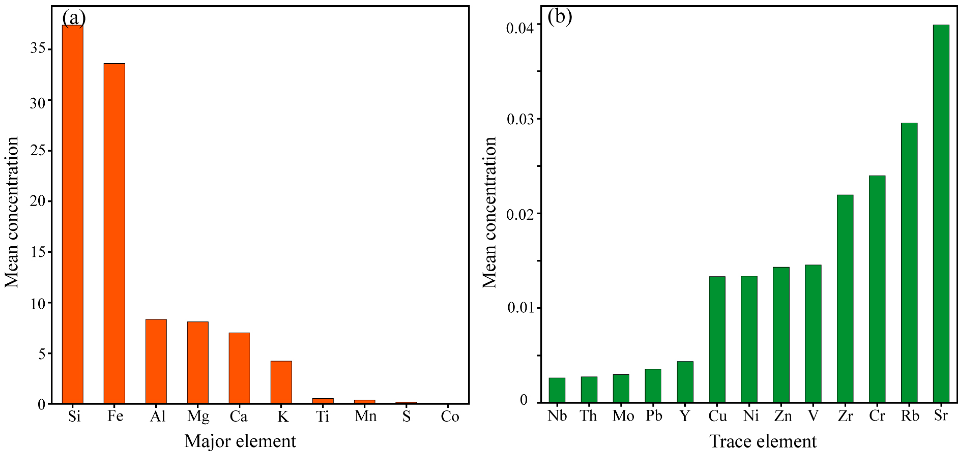
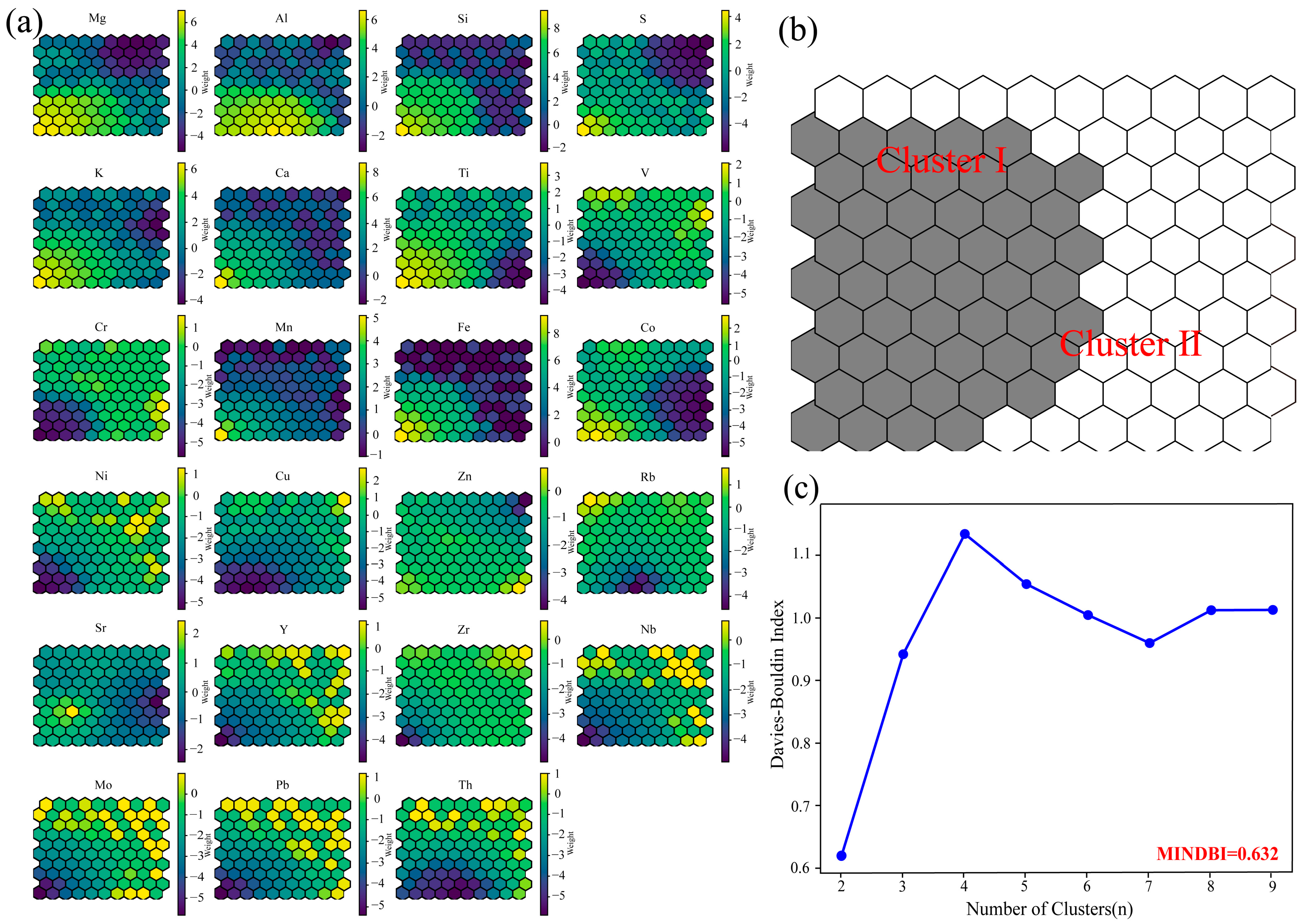
• Self-organizing map (SOM) clustering analysis of X-ray fluorescence (XRF) elemental data from 218 ore samples revealed that the samples from the study area could be divided into two clusters. In the first cluster, elements such as Mg, Al, Si, S, K, Ca, Mn, and Fe exhibited a very strong positive correlation, while Ti, Co, Zn, and Sr showed a weak positive correlation with Fe. Elements such as V, Cr, Ni, Cu, Y, Zr, Nb, Mo, and Pb displayed a negative correlation with Fe. The second cluster consisted of Rb and Th, which showed a positive correlation. Further analysis using TSG shortwave and thermal infrared hyperspectral rock data identified the main mineral types in the mining area, including chlorite, rhodochrosite, dolomite, amphibole, biotite, montmorillonite, quartz, and feldspar. Combined with the XRF results, it was concluded that the region is characterized by significant hydrothermal alteration, primarily chloritization and carbonation, closely related to mineralization. Mg, Al, Si, and Ca were identified as important indicator elements for further deep exploration.
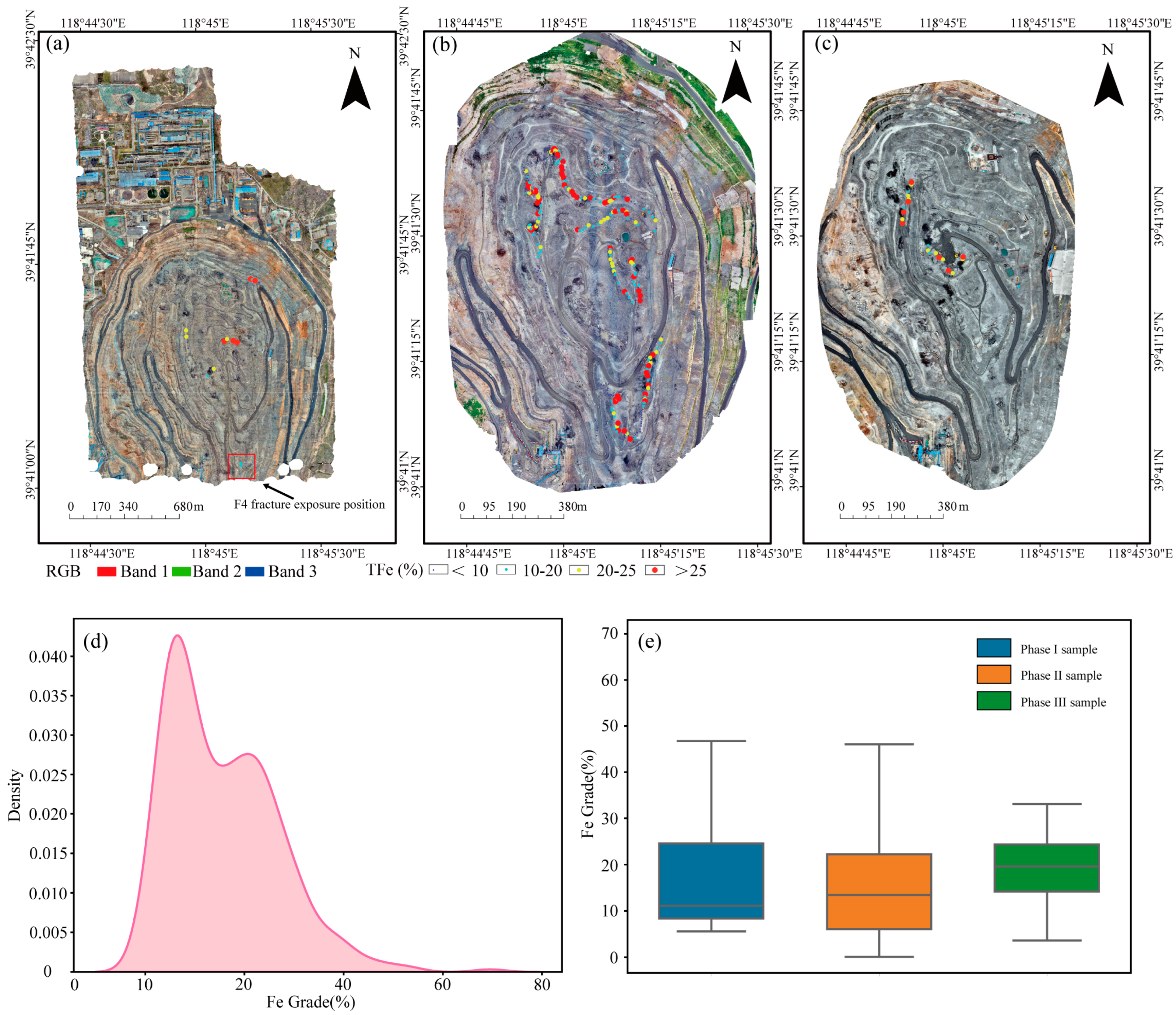
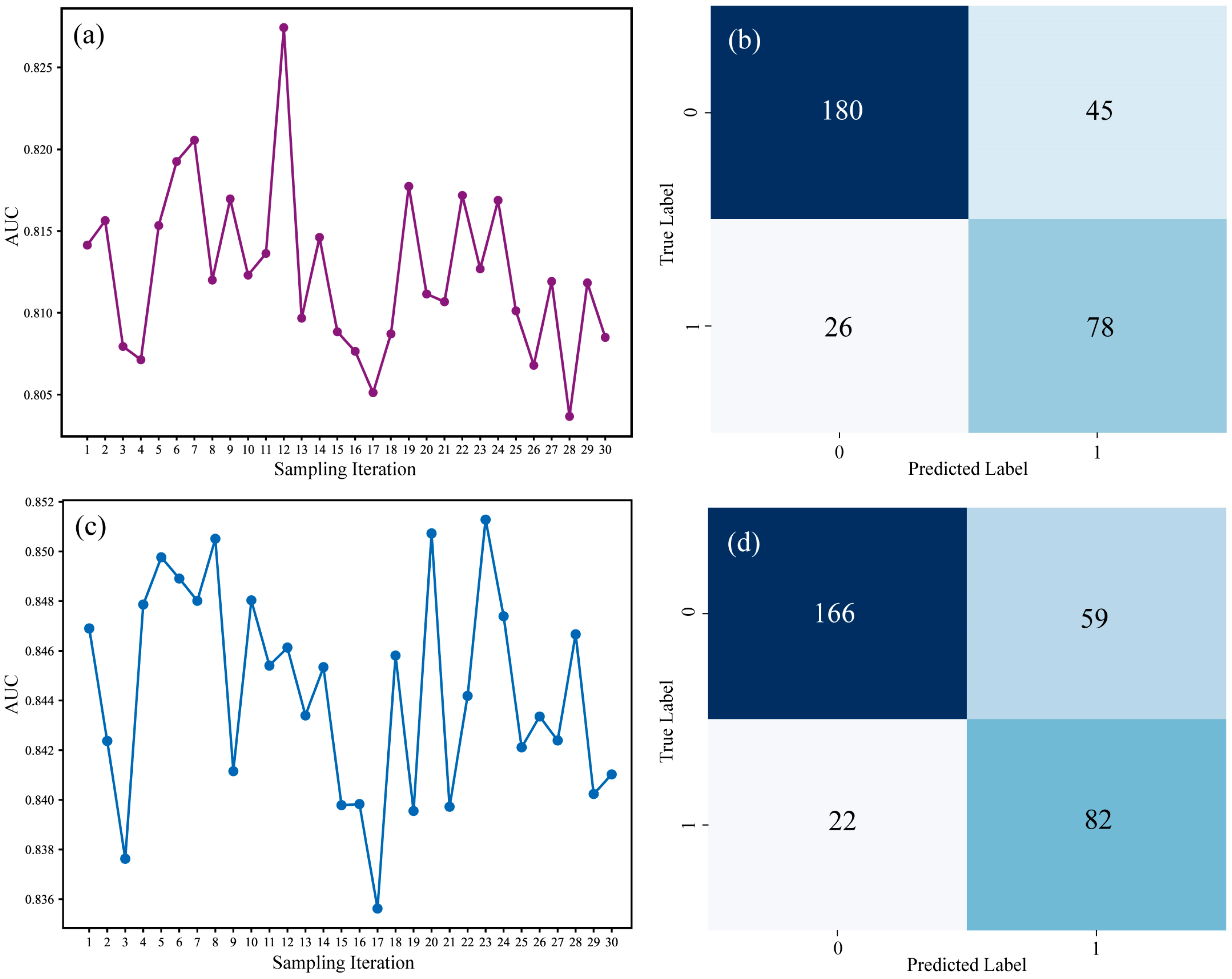
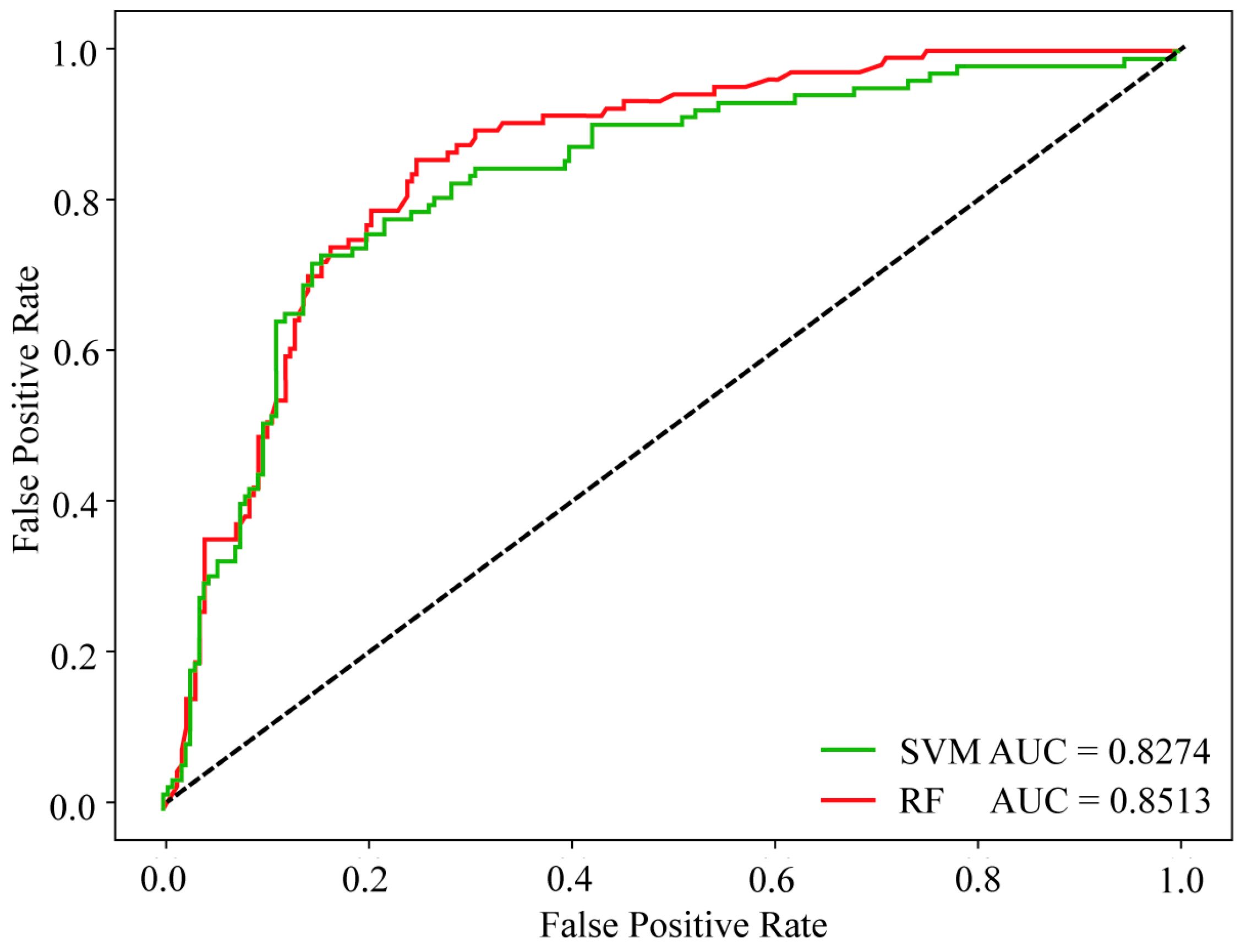
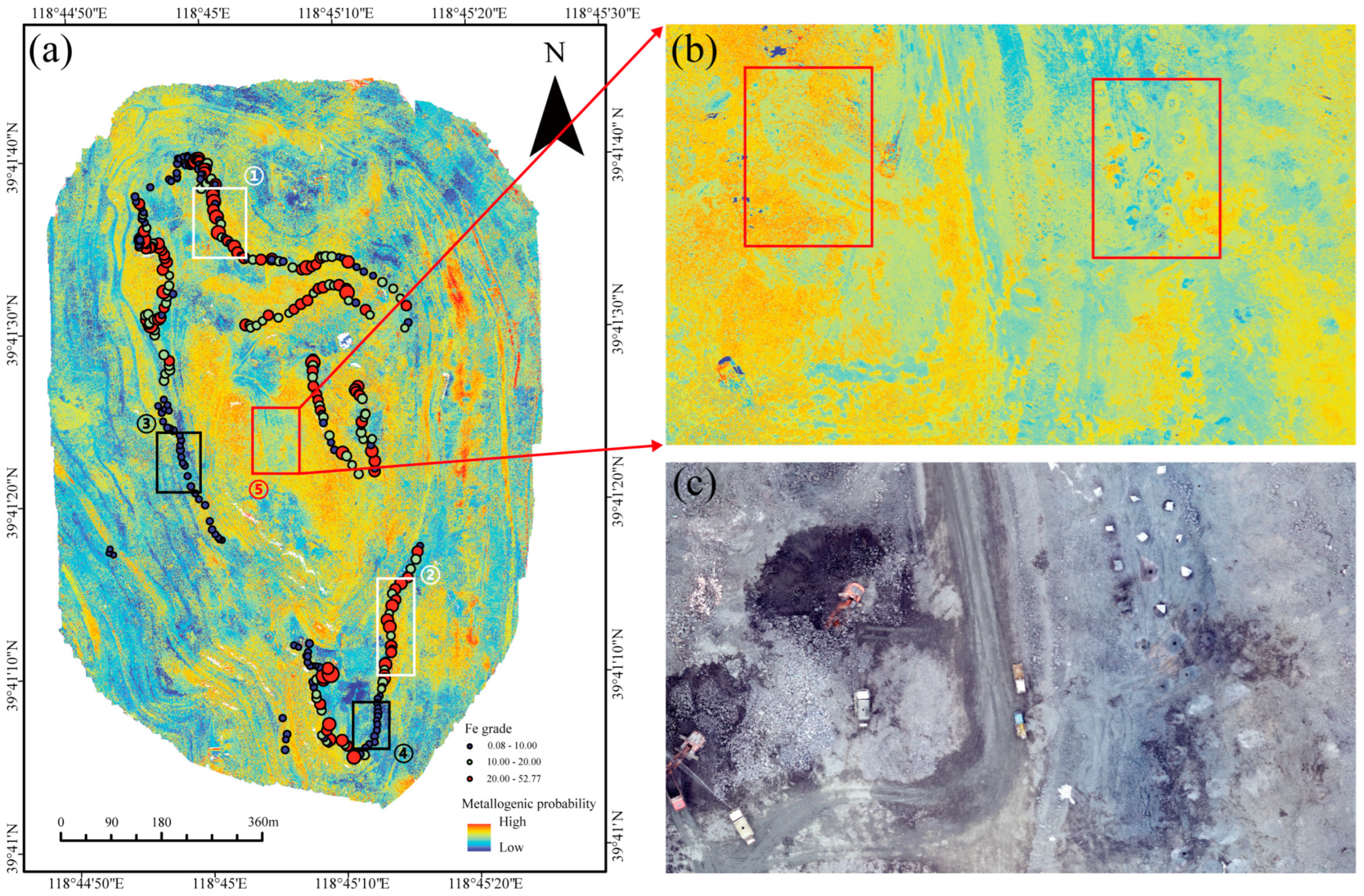
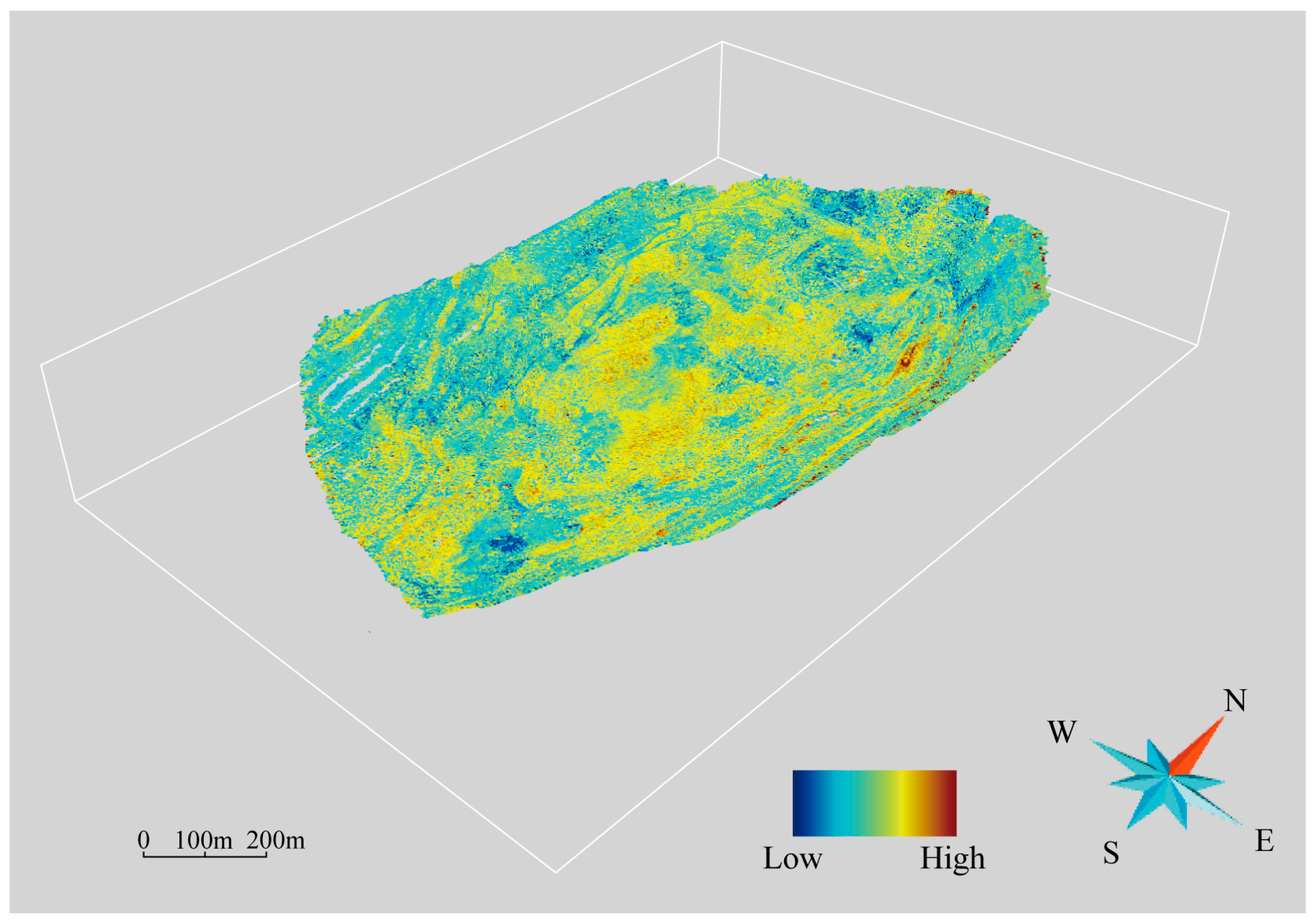
• Based on high-precision drone multispectral data and XRF sample grade data, an ore grade–spectrum correlation model was constructed using Random Forests, Support Vector Machine algorithms, and SMOTE algorithms. After evaluating multiple performance metrics, the RF23 model was selected as the optimal model for real-time prediction of the surface total iron grade in the mining area, with an ore body identification accuracy of 0.79. The model was applied to centimeter-level drone images, achieving high-precision intelligent identification of magnetite in the mining area. The drone multispectral image prediction clearly delineated the boundaries of rock minerals, aligning well with the grade distribution of measured samples, especially in the stope and blasted rock powder areas. Combined with LiDAR image elevation data, real-time monitoring of the three-dimensional surface mineralization information of the mining area was successfully realized, providing significant support for improving ore recovery rates and real-time detection in the mining area, demonstrating great practical application value.
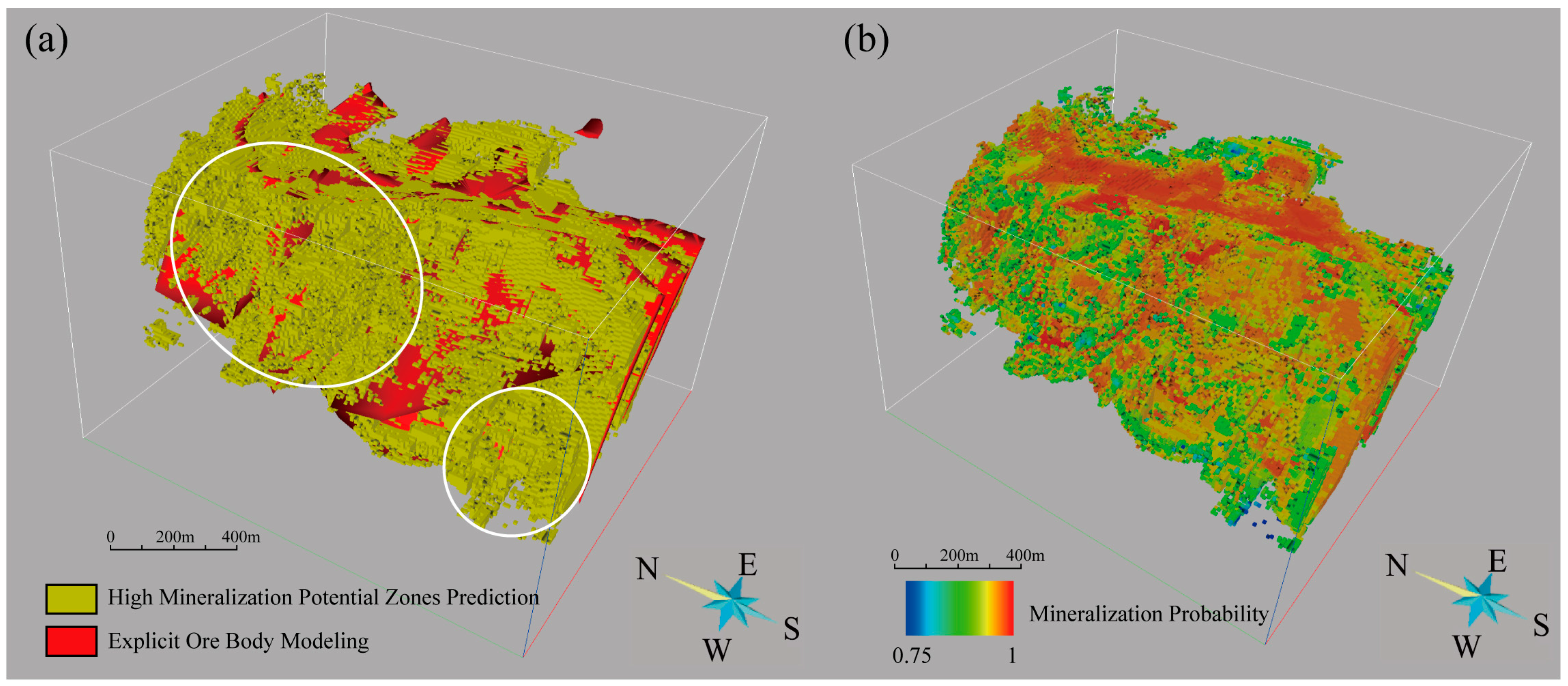
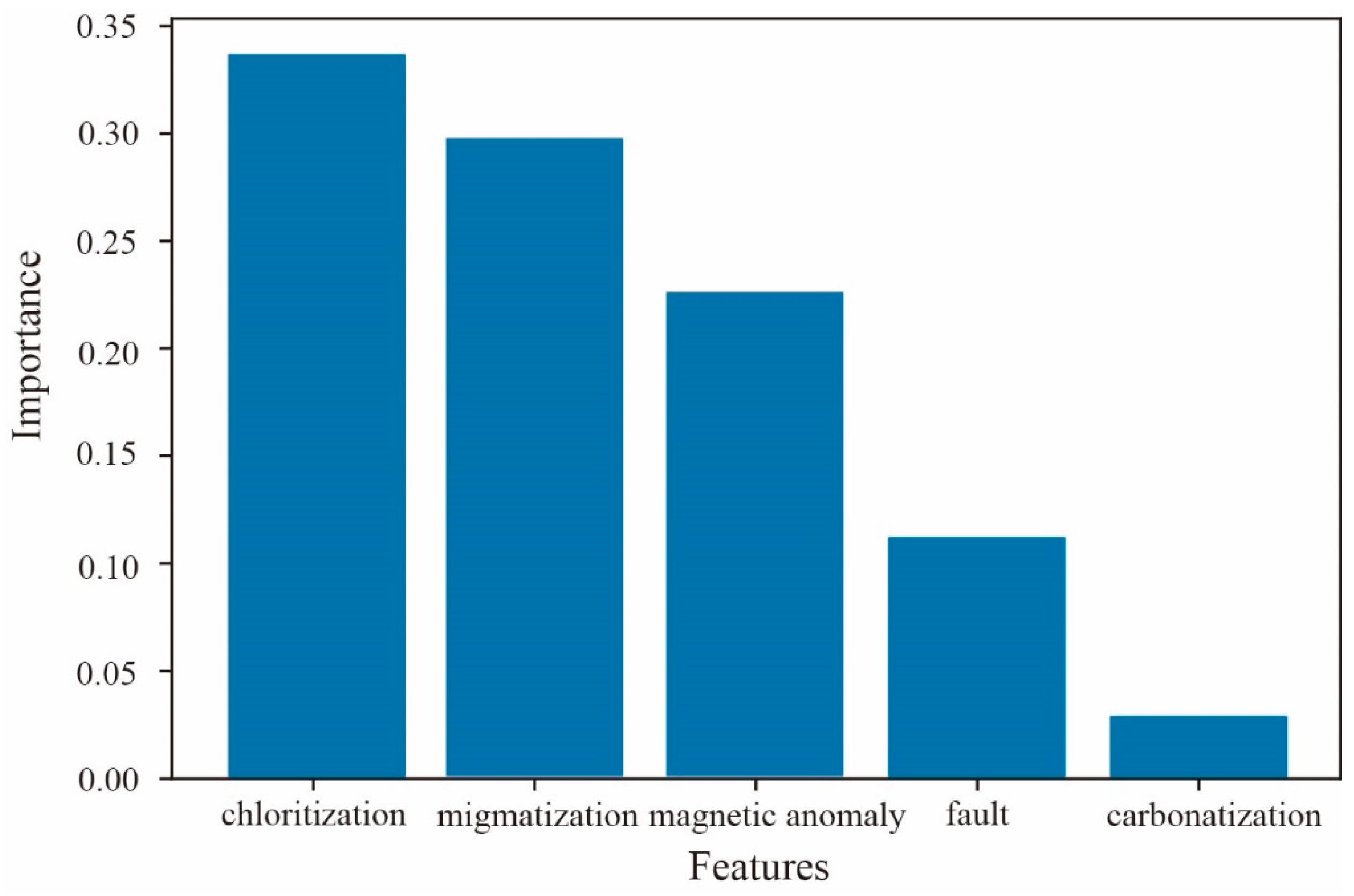
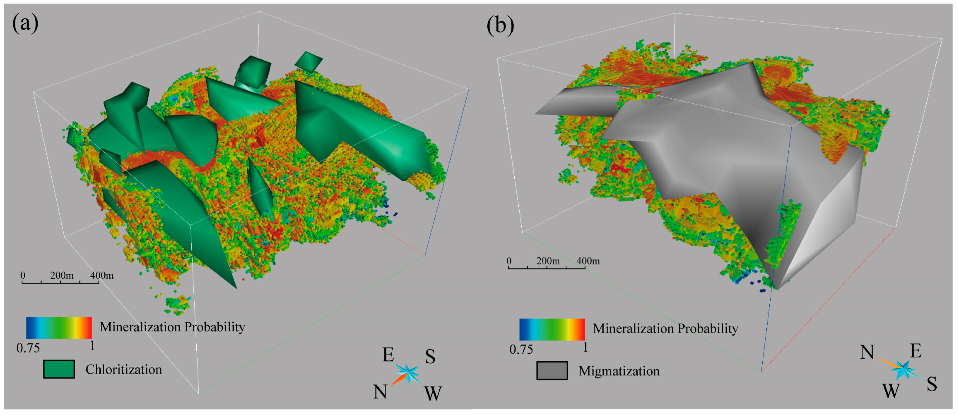
• A three-dimensional geological model was constructed to perform three-dimensional mineral resource potential evaluation (MPM). The results show that the BPUL algorithm can be effectively applied to deep mineral exploration prediction in the Yanshan Iron Mine. The predicted results closely aligned with the spatial location of high-grade mineralization zones. The P-V diagram analysis helped identify the high-mineralization areas at the scale of the mining area, pinpointing two potential exploration targets in the deep and northwest regions. SHAP values and the morphological features of different three-dimensional geological models indicated that chloritization, mixed rock alteration, and magnetic anomalies have significant contributions to ore body enrichment, while faults have some control over the morphological distribution of the Yanshan Iron Mine, but their contribution to the formation of high-grade ore bodies is relatively small.

References

1. Wang, D.H. Study on Critical Mineral Resources: Significance of Research, Determination of Types, Attributes of Resources, Progress of Prospecting, Problems of Utilization, and Direction of Exploitation. Acta Geol. Sin. 2019, 93, 118–1209. [Google Scholar]
2. Zhao, P. “Tri-Linked” Resource Quantitative Prediction and Evaluation: Discussion on Digital Prospecting Theory and Practice. Earth Sci. 2002, 5, 482–489, (In Chinese with English abstract). [Google Scholar]
3. Zhao, P.; Chen, Y. Digital Geology and Digital Mineral Exploration. Earth Sci. Front. 2021, 28, 1–5+434–435, (In Chinese with English abstract). [Google Scholar]
4. Zuo, R.; Xiong, Y. Geodata Science and Geochemical Mapping. J. Geochem. Explor. 2020, 209, 106431. [Google Scholar]
5. Huang, J.; Mao, X.; Deng, H.; Liu, Z.; Chen, J.; Xiao, K. An Improved GWR Approach for Exploring the Anisotropic Influence of Ore-Controlling Factors on Mineralization in 3D Space. Nat. Resour. Res. 2022, 31, 2181–2196. [Google Scholar]
6. Zhang, Z.; Wang, G.; Carranza, E.J.M.; Yang, S.; Zhao, K.; Yang, W.; Sha, D. Three-Dimensional Pseudo-Lithologic Modeling Via Adaptive Feature Weighted k-Means Algorithm from Multi-Source Geophysical Datasets, Qingchengzi Pb–Zn–Ag–Au District, China. Nat. Resour. Res. 2022, 31, 2163–2179. [Google Scholar]
7. Sinaice, B.B.; Owada, N.; Ikeda, H.; Toriya, H.; Bagai, Z.; Shemang, E.; Adachi, T.; Kawamura, Y. Spectral Angle Mapping and AI Methods Applied in Automatic Identification of Placer Deposit Magnetite Using Multispectral Camera Mounted on UAV. Minerals 2022, 12, 268. [Google Scholar] [CrossRef]
8. Zhang, G.; Chen, Q.; Zhao, Z.; Zhang, X.; Chao, J.; Zhou, D.; Chai, W.; Yang, H.; Lai, Z.; He, Y. Nickel Grade Inversion of Lateritic Nickel Ore Using WorldView-3 Data Incorporating Geospatial Location Information: A Case Study of North Konawe, Indonesia. Remote Sens. 2023, 15, 3660. [Google Scholar] [CrossRef]
9. Zhang, L.; Zhang, L.; Du, B. Deep Learning for Remote Sensing Data: A Technical Tutorial on the State of the Art. IEEE Geosci. Remote Sens. Mag. 2016, 4, 22–40. [Google Scholar]
10. Jian, H.; Gong, W.; Li, Y.; Wang, L. Bayesian Inference of Fault Slip and Coupling Along the Tuosuo Lake Segment of the Kunlun Fault, China. Geophys. Res. Lett. 2022, 49, e2021GL096882. [Google Scholar]
11. Yang, J.; Lu, R.; Tao, W.; Cai, M.; Liu, G.; Sun, X. MultiURNet for 3D Seismic Fault Attributes Fusion Detection Combined with PCA. J. Appl. Geophys. 2024, 221, 105296. [Google Scholar] [CrossRef]
12. Yang, J.; Lu, R.; Tao, W.; Liu, G.; Guo, Z.; Yang, X.; Wang, K. Intelligent Identification of Sample-Adaptive Fracture Systems and Seismic Structure Analysis: A Case Study of the Hutubi Gas Storage Field in Xinjiang, China. Seismol. Res. Lett. 2025. [Google Scholar] [CrossRef]
13. Asadzadeh, S.; Chabrillat, S.; Cudahy, T.; Rashidi, B.; De Souza Filho, C.R. Alteration Mineral Mapping of the Shadan Porphyry Cu-Au Deposit (Iran) Using Airborne Imaging Spectroscopic Data: Implications for Exploration Drilling. Econ. Geol. 2024, 119, 139–160. [Google Scholar] [CrossRef]
14. Chen, Q.; Zhao, Z.; Zhou, J.; Zhu, R.; Xia, J.; Sun, T.; Zhao, X.; Chao, J. ASTER and GF-5 Satellite Data for Mapping Hydrothermal Alteration Minerals in the Longtoushan Pb-Zn Deposit, SW China. Remote Sens. 2022, 14, 1253. [Google Scholar] [CrossRef]
15. Lyu, P.; He, L.; He, Z.; Liu, Y.; Deng, H.; Qu, R.; Wang, J.; Zhao, Y.; Wei, Y. Research on Remote Sensing Prospecting Technology Based on Multi-Source Data Fusion in Deep-Cutting Areas. Ore Geol. Rev. 2021, 138, 104359. [Google Scholar]
16. Li, X.; Yuan, F.; Zhang, M.; Jowitt, S.M.; Ord, A.; Zhou, T.; Dai, W. 3D Computational Simulation-Based Mineral Prospectivity Modeling for Exploration for Concealed Fe–Cu Skarn-Type Mineralization within the Yueshan Orefield, Anqing District, Anhui Province, China. Ore Geol. Rev. 2019, 105, 1–17. [Google Scholar] [CrossRef]
17. Huang, J.; Mao, X.; Chen, J.; Deng, H.; Dick, J.M.; Liu, Z. Exploring Spatially Non-Stationary Relationships in the Determinants of Mineralization in 3D Geological Space. Nat. Resour. Res. 2020, 29, 439–458. [Google Scholar] [CrossRef]
18. Mao, X.; Su, Z.; Deng, H.; Liu, Z.; Li, L.; Wang, Y.; Wang, Y.; Wu, L. Three-Dimensional Mineral Prospectivity Modeling with Geometric Restoration: Application to the Jinchuan Ni–Cu–(PGE) Sulfide Deposit, Northwestern China. Nat. Resour. Res. 2024, 33, 75–105. [Google Scholar]
19. Mao, X.; Wang, J.; Deng, H.; Liu, Z.; Chen, J.; Wang, C.; Liu, J. Bayesian Decomposition Modelling: An Interpretable Nonlinear Approach for Mineral Prospectivity Mapping. Math. Geosci. 2023, 55, 897–942. [Google Scholar] [CrossRef]
20. Gao, M.; Wang, G.; Carranza, E.J.M.; Qi, S.; Zhang, W.; Pang, Z.; Li, X.; Xiao, F. 3D Au Targeting Using Machine Learning with Different Sample Combination and Return-Risk Analysis in the Sanshandao-Cangshang District, Shandong Province, China. Nat. Resour. Res. 2024, 33, 51–57. [Google Scholar] [CrossRef]
21. Zhang, C.; Zuo, R. Recognition of Multivariate Geochemical Anomalies Associated with Mineralization Using an Improved Generative Adversarial Network. Ore Geol. Rev. 2021, 136, 104264. [Google Scholar] [CrossRef]
22. Shi, L.; Xu, Y.; Zuo, R. A Heterogeneous Graph Construction Method for Mineral Prospectivity Mapping. Nat. Resour. Res. 2024, 33, 1365–1376. [Google Scholar]
23. He, X.; Zhang, F.; Jim, C.Y.; Chan, N.W.; Tan, M.L.; Shi, J. A New Method to Extract Coal-Covered Area in Open-Pit Mine Based on Remote Sensing. Int. J. Remote Sens. 2024, 45, 5901–5916. [Google Scholar]
24. Carranza, E.J.M.; Laborte, A.G. Random Forest Predictive Modeling of Mineral Prospectivity with Small Number of Prospects and Data with Missing Values in Abra (Philippines). Comput. Geosci. 2015, 74, 60–70. [Google Scholar]
25. Chen, Y.; Wu, W. Application of One-Class Support Vector Machine to Quickly Identify Multivariate Anomalies from Geochemical Exploration Data. Geochem. Explor. Environ. Anal. 2017, 17, 231–238. [Google Scholar]
26. Latifovic, R.; Pouliot, D.; Campbell, J. Assessment of Convolution Neural Networks for Surficial Geology Mapping in the South Rae Geological Region, Northwest Territories, Canada. Remote Sens. 2018, 10, 307. [Google Scholar] [CrossRef]
27. Luo, Z.; Xiong, Y.; Zuo, R. Recognition of Geochemical Anomalies Using a Deep Variational Autoencoder Network. Appl. Geochem. 2020, 122, 104710. [Google Scholar] [CrossRef]
28. Song, S.; Mukerji, T.; Hou, J. GANSim: Conditional Facies Simulation Using an Improved Progressive Growing of Generative Adversarial Networks (GANs). Math. Geosci. 2021, 53, 1413–1444. [Google Scholar] [CrossRef]
29. Keykhay-Hosseinpoor, M.; Kohsary, A.-H.; Hossein-Morshedy, A.; Porwal, A. A Machine Learning-Based Approach to Exploration Targeting of Porphyry Cu-Au Deposits in the Dehsalm District, Eastern Iran. Ore Geol. Rev. 2020, 116, 103234. [Google Scholar]
30. Li, T.; Zuo, R.; Zhao, X.; Zhao, K. Mapping Prospectivity for Regolith-Hosted REE Deposits via Convolutional Neural Network with Generative Adversarial Network Augmented Data. Ore Geol. Rev. 2022, 142, 104693. [Google Scholar]
31. Luo, Z.; Zuo, R. Causal Discovery and Deep Learning Algorithms for Detecting Geochemical Patterns Associated with Gold-Polymetallic Mineralization: A Case Study of the Edongnan Region. Math. Geosci. 2025, 57, 193–220. [Google Scholar] [CrossRef]
32. Deng, H.; Zheng, Y.; Chen, J.; Yu, S.; Xiao, K.; Mao, X. Learning 3D Mineral Prospectivity from 3D Geological Models Using Convolutional Neural Networks: Application to a Structure-Controlled Hydrothermal Gold Deposit. Comput. Geosci. 2022, 161, 105074. [Google Scholar] [CrossRef]
33. Mou, N.; Carranza, E.J.M.; Wang, G.; Sun, X. A Framework for Data-Driven Mineral Prospectivity Mapping with Interpretable Machine Learning and Modulated Predictive Modeling. Nat. Resour. Res. 2023, 32, 2439–2462. [Google Scholar] [CrossRef]
34. Wang, G.; Li, R.; Carranza, E.J.M.; Zhang, S.; Yan, C.; Zhu, Y.; Qu, J.; Hong, D.; Song, Y.; Han, J.; et al. 3D Geological Modeling for Prediction of Subsurface Mo Targets in the Luanchuan District, China. Ore Geol. Rev. 2015, 71, 592–610. [Google Scholar] [CrossRef]
35. Lv, X.; Wang, G. GIS-Based Mineral Prospectivity Mapping Using Machine Learning Methods: A Case Study from Duobaoshan Ore District, Northeastern China. Ore Geol. Rev. 2024, 175, 106352. [Google Scholar] [CrossRef]
36. Luo, Z.; Zuo, R.; Xiong, Y.; Zhou, B. Metallogenic-Factor Variational Autoencoder for Geochemical Anomaly Detection by Ad-Hoc and Post-Hoc Interpretability Algorithms. Nat. Resour. Res. 2023, 32, 835–853. [Google Scholar] [CrossRef]
37. Zhang, Z.; Wang, G.; Carranza, E.J.M.; Liu, C.; Li, J.; Fu, C.; Liu, X.; Chen, C.; Fan, J.; Dong, Y. An Integrated Machine Learning Framework with Uncertainty Quantification for Three-Dimensional Lithological Modeling from Multi-Source Geophysical Data and Drilling Data. Eng. Geol. 2023, 324, 107255. [Google Scholar] [CrossRef]
38. Zhao, G.; Wilde, S.A.; Cawood, P.A.; Lu, L. Thermal Evolution of Archean Basement Rocks from the Eastern Part of the North China Craton and Its Bearing on Tectonic Setting. Int. Geol. Rev. 1998, 40, 706–721. [Google Scholar] [CrossRef]
39. Zhou, X.; Liu, N.; Tang, F.; Zhao, Y.; Qin, K.; Zhang, L.; Li, D. A Deep Manifold Learning Approach for Spatial-Spectral Classification with Limited Labeled Training Samples. Neurocomputing 2019, 331, 138–149. [Google Scholar]
40. Li, H.; Zhang, Z.; Li, L.; Zhang, Z.; Chen, J.; Yao, T. Types and General Characteristics of the BIF-Related Iron Deposits in China. Ore Geol. Rev. 2014, 57, 264–287. [Google Scholar] [CrossRef]
41. Zhang, Z.; Hou, T.; Santosh, M.; Li, H.; Li, J.; Zhang, Z.; Song, X.; Wang, M. Spatio-Temporal Distribution and Tectonic Settings of the Major Iron Deposits in China: An Overview. Ore Geol. Rev. 2014, 57, 247–263. [Google Scholar] [CrossRef]
42. Xu, Y.; Zhang, L.; Gao, X.; Li, H.; Jia, D.; Li, L. Metallogenic conditions of high-grade ores in the Sijiaying sedimentary metamorphic iron deposit, Eastern Hebei Province. Geol. Explor. 2014, 50, 675–688, (In Chinese with English abstract). [Google Scholar]
43. Zhang, T.; Zhang, W.; Wang, Z.; Zhang, F.; Li, B.; Yang, L. Characteristics of Gravity and Magnetic Anomalies in the Luanan Area of Eastern Hebei and Their Significance in Mineral Exploration. Geophys. Geochem. Explor. 2014, 38, 641–648, (In Chinese with English abstract). [Google Scholar]
44. Xu, Y.; Zhang, L.; Li, H.; Li, L.; Gao, X.; Jia, D. The Exploration Model of the Sijiaying Sedimentary Metamorphic Iron Deposit in Eastern Hebei Province. Geol. Explor. 2015, 51, 23–35, (In Chinese with English abstract). [Google Scholar]
45. Zhao, Y. Main genetic types and geological characteristics of iron-rich ore deposits in China. Miner. Depos. 2013, 32, 685–704, (In Chinese with English abstract). [Google Scholar]
46. Gao, X.; Wang, D.; Huang, F.; Wang, Y.; Guo, W. Discussion on deep prospecting of the Sijiaying iron deposit in eastern Hebei Province. Acta Geol. Sin. 2022, 96, 2495–2505, (In Chinese with English abstract). [Google Scholar]
47. Zhang, L.; Zhai, M.; Wan, Y.; Guo, J.; Dai, Y.; Wang, C.; Liu, L. Study of the Precambrian BF-iron depositsin the North China Craton: Progresses and questions. Acta Petrol. Sin. 2012, 28, 3431–3445, (In Chinese with English abstract). [Google Scholar]
48. Li, W.; Dong, G.; Ding, F.; Cao, R.; Yang, L.; Fan, Y.; Liu, J.; Zheng, X. Mineralogical characteristics of typical ore from the BlF-type iron deposit at Sijiaying north mining district in eastern Hebei Province and their constraints on the metallogenic evolution. Acta Petrol. Mineral. 2025, 44, 68–86, (In Chinese with English abstract). [Google Scholar]
49. Moreira, A.; Prats-Iraola, P.; Younis, M.; Krieger, G.; Hajnsek, I.; Papathanassiou, K.P. A Tutorial on Synthetic Aperture Radar. IEEE Geosci. Remote Sens. Mag. 2013, 1, 6–43. [Google Scholar]
50. Jackisch, R.; Lorenz, S.; Kirsch, M.; Zimmermann, R.; Tusa, L.; Pirttijärvi, M.; Saartenoja, A.; Ugalde, H.; Madriz, Y.; Savolainen, M.; et al. Integrated Geological and Geophysical Mapping of a Carbonatite-Hosting Outcrop in Siilinjärvi, Finland, Using Unmanned Aerial Systems. Remote Sens. 2020, 12, 2998. [Google Scholar] [CrossRef]
51. Li, B.; Peng, Y.; Zhao, X.; Liu, X.; Wang, G.; Jiang, H.; Wang, H.; Yang, Z. Combining 3D Geological Modeling and 3D Spectral Modeling for Deep Mineral Exploration in the Zhaoxian Gold Deposit, Shandong Province, China. Minerals 2022, 12, 1272. [Google Scholar] [CrossRef]
52. Zuo, L.; Wang, G.; Carranza, E.J.M.; Zhai, D.; Pang, Z.; Cao, K.; Mou, N.; Huang, L. Short-Wavelength Infrared Spectral Analysis and 3D Vector Modeling for Deep Exploration in the Weilasituo Magmatic–Hydrothermal Li–Sn Polymetallic Deposit, Inner Mongolia, NE China. Nat. Resour. Res. 2022, 31, 3121–3153. [Google Scholar]
53. Zuo, L.; Wang, G.; Carranza, E.J.M.; Pang, Z.; Ren, H.; Cao, K.; Liu, Z.; Gao, M. Deep Vector Exploration via Alteration Footprints and Thermal Infrared Scalars for the Weilasituo Magmatic–Hydrothermal Li–Sn Polymetallic Deposit, Inner Mongolia, NE China. Nat. Resour. Res. 2023, 32, 1871–1895. [Google Scholar]
54. Shao, X.; Peng, Y.; Wang, G.; Zhao, X.; Tang, J.; Huang, L.; Liu, X.; Zhao, X. Application of Shortwave Infrared Spectroscopy, X-ray Fluorescence Spectroscopy, and Pyrite Thermoelectric Analysis in Deep Exploration of the Jincheng Gold Mine Field in Jiaodong. Earth Sci. Front. 2021, 28, 236–251, (In Chinese with English abstract). [Google Scholar]
55. Kohonen, T. Self-Organized Formation of Topologically Correct Feature Maps. Biol. Cybern. 1982, 43, 59–69. [Google Scholar]
56. Guo, G.; Li, K.; Zhang, D.; Lei, M. Quantitative Source Apportionment and Associated Driving Factor Identification for Soil Potential Toxicity Elements via Combining Receptor Models, SOM, and Geo-Detector Method. Sci. Total Environ. 2022, 830, 154721. [Google Scholar]
57. Rahimi, H.; Abedi, M.; Yousefi, M.; Bahroudi, A.; Elyasi, G.-R. Supervised Mineral Exploration Targeting and the Challenges with the Selection of Deposit and Non-Deposit Sites Thereof. Appl. Geochem. 2021, 128, 104940. [Google Scholar] [CrossRef]
58. Hazenfratz, R.; Munita, C.S.; Neves, E.G. Neural Networks (SOM) Applied to INAA Data of Chemical Elements in Archaeological Ceramics from Central Amazon. STAR: Sci. Technol. Archaeol. Res. 2017, 3, 334–340. [Google Scholar]
59. Li, Y.; Wright, A.; Liu, H.; Wang, J.; Wang, G.; Wu, Y.; Dai, L. Land Use Pattern, Irrigation, and Fertilization Effects of Rice-Wheat Rotation on Water Quality of Ponds by Using Self-Organizing Map in Agricultural Watersheds. Agric. Ecosyst. Environ. 2019, 272, 155–164. [Google Scholar]
60. Hariharan, S.; Tirodkar, S.; Porwal, A.; Bhattacharya, A.; Joly, A. Random Forest-Based Prospectivity Modelling of Greenfield Terrains Using Sparse Deposit Data: An Example from the Tanami Region, Western Australia. Nat. Resour. Res. 2017, 26, 489–507. [Google Scholar]
61. Li, T.; Xia, Q.; Zhao, M.; Gui, Z.; Leng, S. Prospectivity Mapping for Tungsten Polymetallic Mineral Resources, Nanling Metallogenic Belt, South China: Use of Random Forest Algorithm from a Perspective of Data Imbalance. Nat. Resour. Res. 2020, 29, 203–227. [Google Scholar]
62. Peng, Q.; Wang, Z.; Wang, G.; Zhang, W.; Chen, Z.; Liu, X. 3D Mineral Prospectivity Mapping from 3D Geological Models Using Return–Risk Analysis and Machine Learning on Imbalance Data. Minerals 2023, 13, 1384. [Google Scholar] [CrossRef]
63. Chawla, N.V.; Bowyer, K.W.; Hall, L.O.; Kegelmeyer, W.P. SMOTE: Synthetic Minority Over-Sampling Technique. J. Artif. Intell. Res. 2002, 16, 321–357. [Google Scholar]
64. Cortes, C.; Vapnik, V. Support-Vector Networks. Mach. Learn. 1995, 20, 273–297. [Google Scholar]
65. Ge, Y.-Z.; Zhang, Z.-J.; Cheng, Q.-M.; Wu, G.-P. Geological Mapping of Basalt Using Stream Sediment Geochemical Data: Case Study of Covered Areas in Jining, Inner Mongolia, China. J. Geochem. Explor. 2022, 232, 106888. [Google Scholar]
66. Carranza, E.J.M.; Laborte, A.G. Data-Driven Predictive Mapping of Gold Prospectivity, Baguio District, Philippines: Application of Random Forests Algorithm. Ore Geol. Rev. 2015, 71, 777–787. [Google Scholar]
67. Gao, M.; Wang, G.; Yang, W.; Zhang, Z.; Cai, D.; Xu, Y.; Yang, S. Bagging-Based Positive–Unlabeled Data Learning Algorithm with Base Learners Random Forest and XGBoost for 3D Exploration Targeting in the Kalatongke District, Xinjiang, China. Nat. Resour. Res. 2023, 32, 437–459. [Google Scholar]
68. Jia, R.; Lv, Y.; Wang, G.; Carranza, E.J.M.; Chen, Y.; Wei, C.; Zhang, Z. A Stacking Methodology of Machine Learning for 3D Geological Modeling with Geological-Geophysical Datasets, Laochang Sn Camp, Gejiu (China). Comput. Geosci. 2021, 151, 104754. [Google Scholar]
69. Mou, N.; Wang, G.; Sun, X. Identification of Geochemical Anomalies Related to Mineralization: A Case Study from Porphyry Copper Deposits in the Qulong-Jiama Mining District of Tibet, China. J. Geochem. Explor. 2023, 244, 107126. [Google Scholar]
70. Zhang, Z.; Wang, G.; Liu, C.; Cheng, L.; Sha, D. Bagging-Based Positive-Unlabeled Learning Algorithm with Bayesian Hyperparameter Optimization for Three-Dimensional Mineral Potential Mapping. Comput. Geosci. 2021, 154, 104817. [Google Scholar]
71. Zhang, W.; Wu, C.; Zhong, H.; Li, Y.; Wang, L. Prediction of Undrained Shear Strength Using Extreme Gradient Boosting and Random Forest Based on Bayesian Optimization. Geosci. Front. 2021, 12, 469–477. [Google Scholar] [CrossRef]
72. Xia, Y.; Liu, C.; Li, Y.; Liu, N. A Boosted Decision Tree Approach Using Bayesian Hyper-Parameter Optimization for Credit Scoring. Expert Syst. Appl. 2017, 78, 225–241. [Google Scholar] [CrossRef]
73. Wang, Z.; Yin, Z.; Caers, J.; Zuo, R. A Monte Carlo-Based Framework for Risk-Return Analysis in Mineral Prospectivity Mapping. Geosci. Front. 2020, 11, 2297–2308. [Google Scholar] [CrossRef]
74. Bharti, J.P.; Mishra, P.; Moorthy, U.; Sathishkumar, V.E.; Cho, Y.; Samui, P. Slope Stability Analysis Using Rf, Gbm, Cart, Bt and Xgboost. Geotech. Geol. Eng. 2021, 39, 3741–3752. [Google Scholar] [CrossRef]
75. Chen, G.; Huang, N.; Wu, G.; Luo, L.; Wang, D.; Cheng, Q. Mineral Prospectivity Mapping Based on Wavelet Neural Network and Monte Carlo Simulations in the Nanling W-Sn Metallogenic Province. Ore Geol. Rev. 2022, 143, 104765. [Google Scholar] [CrossRef]
76. Xiong, Y.; Zuo, R. A Positive and Unlabeled Learning Algorithm for Mineral Prospectivity Mapping. Comput. Geosci. 2021, 147, 104667. [Google Scholar] [CrossRef]
77. Yousefi, M.; Carranza, E.J.M. Prediction–Area (P–A) Plot and C–A Fractal Analysis to Classify and Evaluate Evidential Maps for Mineral Prospectivity Modeling. Comput. Geosci. 2015, 79, 69–81. [Google Scholar] [CrossRef]
78. Xiao, F.; Chen, J.; Hou, W.; Wang, Z.; Zhou, Y.; Erten, O. A Spatially Weighted Singularity Mapping Method Applied to Identify Epithermal Ag and Pb-Zn Polymetallic Mineralization Associated Geochemical Anomaly in Northwest Zhejiang, China. J. Geochem. Explor. 2018, 189, 122–137. [Google Scholar] [CrossRef]
79. Zuo, R. Identification of Weak Geochemical Anomalies Using Robust Neighborhood Statistics Coupled with GIS in Covered Areas. J. Geochem. Explor. 2014, 136, 93–101. [Google Scholar] [CrossRef]
80. Xue, Q.; Wang, R.; Liu, S.; Shi, W.; Tong, X.; Li, Y.; Sun, F. Significance of Chlorite Hyperspectral and Geochemical Characteristics in Exploration: A Case Study of the Giant Qulong Porphyry Cu-Mo Deposit in Collisional Orogen, Southern Tibet. Ore Geol. Rev. 2021, 134, 104156. [Google Scholar] [CrossRef]
81. Xiao, B.; Chu, G.; Feng, Y. Short-Wave Infrared (SWIR) Spectral and Geochemical Characteristics of Hydrothermal Alteration Minerals in the Laowangou Au Deposit: Implications for Ore Genesis and Vectoring. Ore Geol. Rev. 2021, 139, 104463. [Google Scholar] [CrossRef]
82. Zhao, P. Characteristics of Geological Big Data and Its Rational Development and Utilization. Earth Sci. Front. 2019, 26, 1–5, (In Chinese with English abstract). [Google Scholar]
83. Zhao, P. Big Data Era: Digital Prospecting and Quantitative Evaluation. Geol. Bull. 2015, 34, 1255–1259, (In Chinese with English abstract). [Google Scholar]
84. Wang, C.; Wang, G.; Liu, J.; Zhang, D. 3D Geochemical Modeling for Subsurface Targets of Dashui Au Deposit in Western Qinling (China). J. Geochem. Explor. 2019, 203, 59–77. [Google Scholar]
85. Gao, X.; Wang, D.; Huang, F.; Wang, Y.; Wang, C. Chronolgy and Geochemistry of the Sijiaying Iron Deposit in Eastern Hebei Province, North China Craton: Implications for the Genesis of High-Grade Iron Ores. Minerals 2023, 13, 775. [Google Scholar] [CrossRef]
Figure 1. (a) Tectonic subdivision of the North China Craton and location of the study area in the southern margin of the Craton; (b) geological map of the Sijiaying BIF iron deposit; (c) geological A–B cross-section of the Yanshan BIF.
Applsci 15 04082 g001
Figure 2. Digital Surface Model of Yanshan Iron Mine Open-Pit: (a) Global model of the open-pit; (b) Mixed ore and surrounding rock in the western part of the open-pit; (c) Northeastern slope of the open-pit; (d) Key mining area at the central-bottom section of the open-pit.
Applsci 15 04082 g002
Figure 3. Spatial distribution maps of the three stages of sampling and iron grade distribution of samples: (a) samples collected in April 2023; (b) samples collected in September 2023; (c) samples collected in May 2024; (d) kernel density of iron grades for all samples; (e) box plot of iron grades for samples from each stage.
Applsci 15 04082 g003
Figure 4. UAV multispectral imagery: (a) image of April 2023; (b) image of September 2023; (c) image of May 2024.
Applsci 15 04082 g004
Figure 5. Reduced-to-the-pole (RTP) aeromagnetic anomaly map.
Applsci 15 04082 g005
Figure 6. Yanshan Iron Ore Mine big data integration and multi-dimensional ore-forming prediction process flowchart.
Applsci 15 04082 g006
Figure 7. SOM schematic diagram.
Applsci 15 04082 g007
Figure 8. SMOTE schematic diagram.
Applsci 15 04082 g008
Figure 9. Statistical analysis of the (a) major elements and (b) trace elements.
Applsci 15 04082 g009
Figure 10. (a) SOM clustering results map; (b) clustering of categories map of all output space; (c) Davies–Bouldin index diagram.
Applsci 15 04082 g010
Figure 11. Spectrum TSG interpretation of mineral identification results: (a) shortwave infrared interpretation results, (b) thermal infrared interpretation results.
Applsci 15 04082 g011
Figure 12. (a) Spectral of typical magnetite sample; (b) magnetite spectral characteristics from the USGS spectral library.
Applsci 15 04082 g012
Figure 13. The Spearman correlation map of bands and band ratios. (The red box is the feature correlation coefficient with high correlation with Fe element, positive number is positive correlation, negative number is negative correlation).
Applsci 15 04082 g013
Figure 14. AUC values from thirty rounds of training using Support Vector Machine (a) and Random Forest (c) models, along with the confusion matrix for SVM12 (d) and RF23 (b).
Applsci 15 04082 g014
Figure 15. Optimal ROC curves of SVM12 and RF23.
Applsci 15 04082 g015
Figure 16. Magnetite identification results ((a) identification results for the whole region (Regions 1 and 2 are high mineralization areas, 3 and 4 are low mineralization areas, and 5 are enlarged interception areas); (b) local recognition result; (c) local DOM image corresponding location).
Applsci 15 04082 g016
Figure 17. Three-dimensional magnetite intelligent detection results.
Applsci 15 04082 g017
Figure 18. Three-dimensional deposit-scale model of the (a) carbonatization, (b) chloritization, (c) migmatization, (d) F4 fault, (e) ore body.
Applsci 15 04082 g018
Figure 19. Three-dimensional stratigraphic model.
Applsci 15 04082 g019
Figure 20. Three-dimensional deposit-scale model of the (a) proximity of carbonatization, (b) chloritization, (c) migmatization, (d) fault, (e) magnetic anomaly.
Applsci 15 04082 g020
Figure 21. (a) ROC curve for the BPUL models; (b) P-V plot of the BPUL predictive model.
Applsci 15 04082 g021
Figure 22. (a) Validation of BPUL model’s high mineralization zones against known ore deposits via P-V plot analysis; (b) mineralization probability assessment of high-potential zones in BPUL predictive model.
Applsci 15 04082 g022
Figure 23. Feature importance histogram for BPUL model.
Applsci 15 04082 g023
Figure 24. Comparative results of high-mineralization zones in BPUL predictive model with (a) chloritization and (b) migmatization.
Applsci 15 04082 g024