Spectral Information Divergence-Driven Diffusion Networks for Hyperspectral Target Detection

Abstract

Hyperspectral Imagery (HSI) plays a crucial role in military and civilian target detection. However, HSI target detection remains highly challenging due to the interference caused by complex and diverse real-world scenarios. This paper proposes a Spectral Information Divergence-driven Diffusion Network model (SID-DN) for hyperspectral target detection, which significantly enhances detection robustness in complex scenes by decoupling background distribution modeling from target detection. The proposed method focuses on learning the background distribution in hyperspectral data and achieves target detection by accurately reconstructing background samples to identify differences between background and target samples. This method introduces an adaptive coarse detection module, which optimizes the coarse detection process in generative hyperspectral target detection, effectively reducing the background-target misclassification. Additionally, a SID-based Diffusion model is designed to optimize the loss of Diffusion, effectively reducing the interference of suspected target samples during the background learning process. Experiments on three real-world datasets demonstrate that the method is highly competitive, with detection results significantly outperforming current state-of-the-art methods.

1. Introduction

The growing number of remote sensing satellites and the miniaturization of remote sensing equipment in recent years have enhanced the flexibility of remote sensing data acquisition, enabling quicker and more targeted responses to specific areas [1]. Among various remote sensing technologies, Hyperspectral Imagery (HSI) has attracted significant attention due to its capacity for capturing the distinct spectral properties of different objects in a scene. Hyperspectral sensors can provide hundreds of continuous spectral data across the electromagnetic spectrum, from the visible to the infrared (IR) bands. This enables the accurate observation of the reflection or emission characteristics of the object being tested [2]. Therefore, hyperspectral is capable of a wide range of vision tasks, including image classification [3], anomalous target detection [4], target detection [5], and change detection [6]. Furthermore, it plays a pivotal role in numerous practical applications, including land cover classification [7,8], sea and land military target detection [9], mineral resources exploration [10], and crop pathology detection [11], among others.

Hyperspectral Target Detection (HTD) identifies targets in complex backgrounds by exploiting subtle spectral differences between the targets and backgrounds in HSI. Because of impediments such as cloud cover and the poor spatial resolution of HSI, detected targets are often represented at a sub-pixel level, making the extraction process challenging. HTD methods are primarily divided into classical detection techniques and deep learning-based methods.

The classical HTD methods primarily include methods based on spectral angle detection [12], hypothesis testing [13], Constrained Energy Minimization (CEM) [14], signal decomposition [15] and sparse representation [16]. Spectral angle detection methods measure spectral similarity through geometric or probabilistic metrics, such as Spectral Angle Mapper (SAM) [12], Adaptive Coherence Estimator(ACE) [17] and Spectral Information Divergence (SID) [18].These methods are sensitive to spectral variations and often serve as pre- or post-processing steps due to their computational simplicity [19].Hypothesis testing-based detectors, including Adaptive Spatial Detector (ASD) [20] and Kernel-based Adaptive Subspace Detector (KASD) [21], rely on statistical signal theory and likelihood ratio tests but face limitations from Gaussian distribution assumptions. The CEM detection algorithm [14], minimizes background energy while enhancing target responses through linear filtering. Though simple, its linear nature struggles with nonlinear HSI features, prompting nonlinear extensions like hCEM [22] and machine learning variants [23,24].The Signal Decomposition Detection method [25,26] separate targets from backgrounds using models like Orthogonal Subspace Projection (OSP) [27] and Low-Rank and Sparse Matrix Decomposition (LRaSMD) [28], yet require precise spectral modeling and suffer from high complexity.The sparse representation methods [29,30,31] leverage sparse coefficients and dictionary learning (e.g., a dual sparsity constrained(DSC) [32]) to enhance target-background discrimination. While effective, their performance depends heavily on dictionary completeness, limiting generalization.Most traditional detection algorithms rely on manually predefined assumptions (e.g., spectral matching criteria, energy minimization, or distribution models) and struggle to effectively handle the nonlinear characteristics inherent in complex real-world scenarios. This limitation has driven researchers to explore and adopt end-to-end deep learning models, leveraging data-driven approaches to reduce reliance on handcrafted feature engineering.

Recently, the rapid advancements in deep learning have revitalized HTD. Deep learning can capture complex and diverse nonlinear characteristics of HSI using multi-layered network structures. Deep learning-based HTD methods can be categorized into two main approaches. The first approach constructed an end-to-end network for HSI to enable target detection across all images. Freitas et al. [33] developed a detection model using a 3D Convolutional Neural Network (CNN) for maritime HTD. Zhang et al. [34] introduced HTD-Net, a method combining an Auto Encoder (AE) with CNN for HTD in scenarios with missing labels. Qin et al. [35] introduced the HTD-ViT algorithm, which integrated spectral and spatial information for HTD. Jiao et al. [36] combined Fourier transform with Transformer to develop a dual-branch Fourier hybrid transform network. Wang et al. [37] innovatively enhanced spectral feature learning by integrating the momentum encoder with Transformer. Jiao et al. [38] introduced a triplet spectral transformer method for HTD, excelling at capturing long-term dependencies in spectral features.

The second approach involved reconstructing hyperspectral data using generative deep learning, followed by target detection based on differences between the reconstructed target and background. These methods typically relied on learning from background samples generated after coarse detection. With advancements in generative networks, Generative Adversarial Networks (GAN) [39], Variational Auto Encoders (VAE) [40], and AEs have been widely applied in HTD. Xie et al. [41] pioneered the field by proposing a target-constrained background GAN model, which relies on background learning based on target suppression constraint (BLTSC) for HTD. Xie et al. [42] introduced an unsupervised algorithm leveraging a deep latent spectral representation model to adaptively map latent representations to optimal subset relationships. Ali et al. [43] proposed a self-supervised background learning method by combining principal component analysis (PCA) with an adversarial autoencoder (AAE) network. Xie et al. [44] proposed a Spectral Regularized Unsupervised Network (SRUN) to enhance the spectral representation capabilities of Autoencoder and Variational Autoencoder (VAE) models. The framework integrated spectral angular difference-driven feature selection and adaptive weighting mechanisms to generate discriminative detection maps. Tian et al. [45] combined OSP theory with VAE and proposed the OS-VAE network framework, exploring new methods that fuse traditional methods with deep learning.In order to improve non-linear feature expression and physical interpretability, Shen et al. [46] designed a subspace representation network for HTD. Shi et al. successively integrated AE with HTD to develop the DCSSAE network [47] and 3DMMRAE network [48].

Despite the significant success of deep learning-based HTD, several challenges remain:

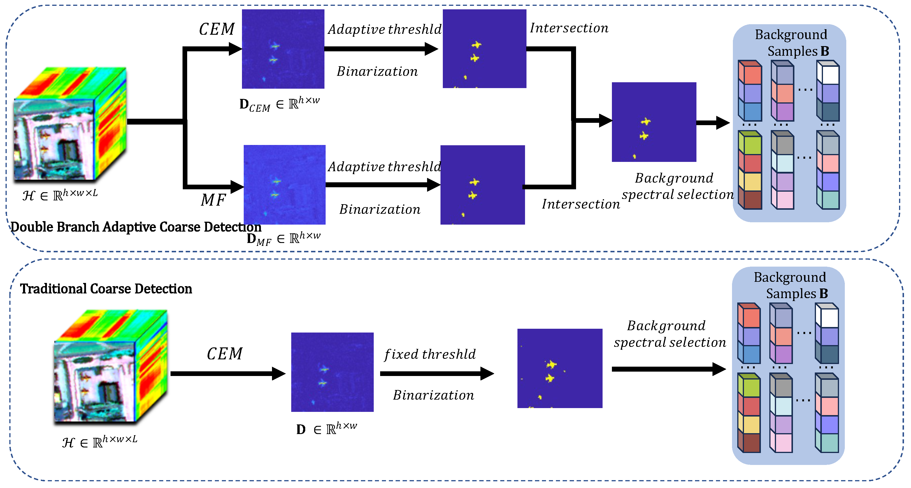
• Supervised deep learning often demands extensive labeled training data, which is challenging to obtain in practical scenarios, potentially undermining its robustness. Recently, self-supervised generative HTD has advanced significantly, but coarse detection often suffers from background-target misclassification. Improving coarse detection remains a critical challenge in generative HTD.
• Effective background learning is crucial for enhancing algorithm performance through improved background representation. However, HSI is often underestimated in practical applications, with its relationship to prior spectra poorly understood, leading to inadequate suppression of specific targets.

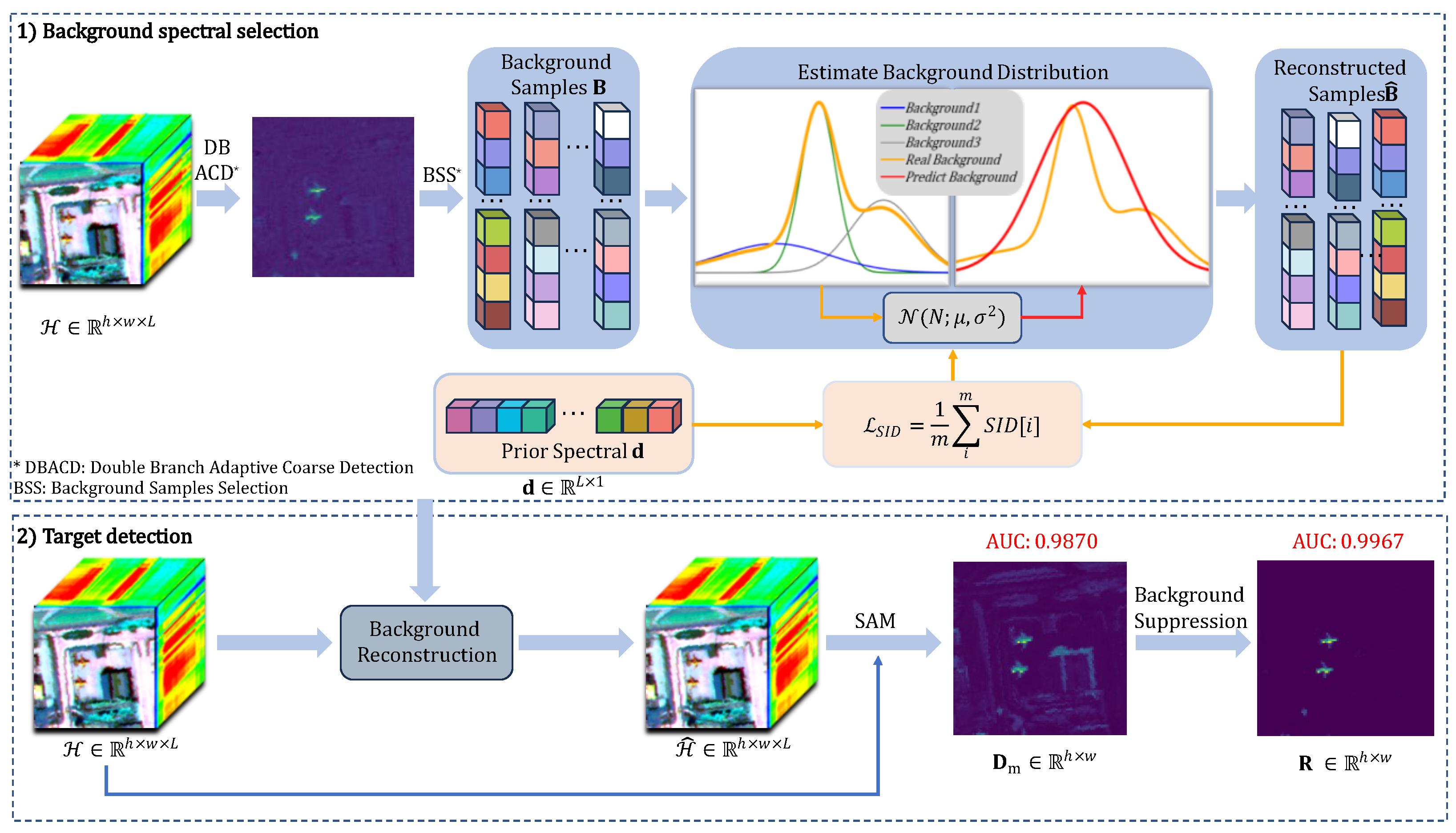
Based on the above considerations, this paper proposes a hyperspectral detection deep learning model based on Diffusion and target suppression constraints, with the intention of enhancing coarse detection’s efficiency and the ability to represent the background. The model is named by SID-DN. The main contributions of this paper are as follows:

• This paper proposes a two-stream adaptive coarse detection algorithm that enhances the coarse detection process and better distinguishes background samples from target samples.
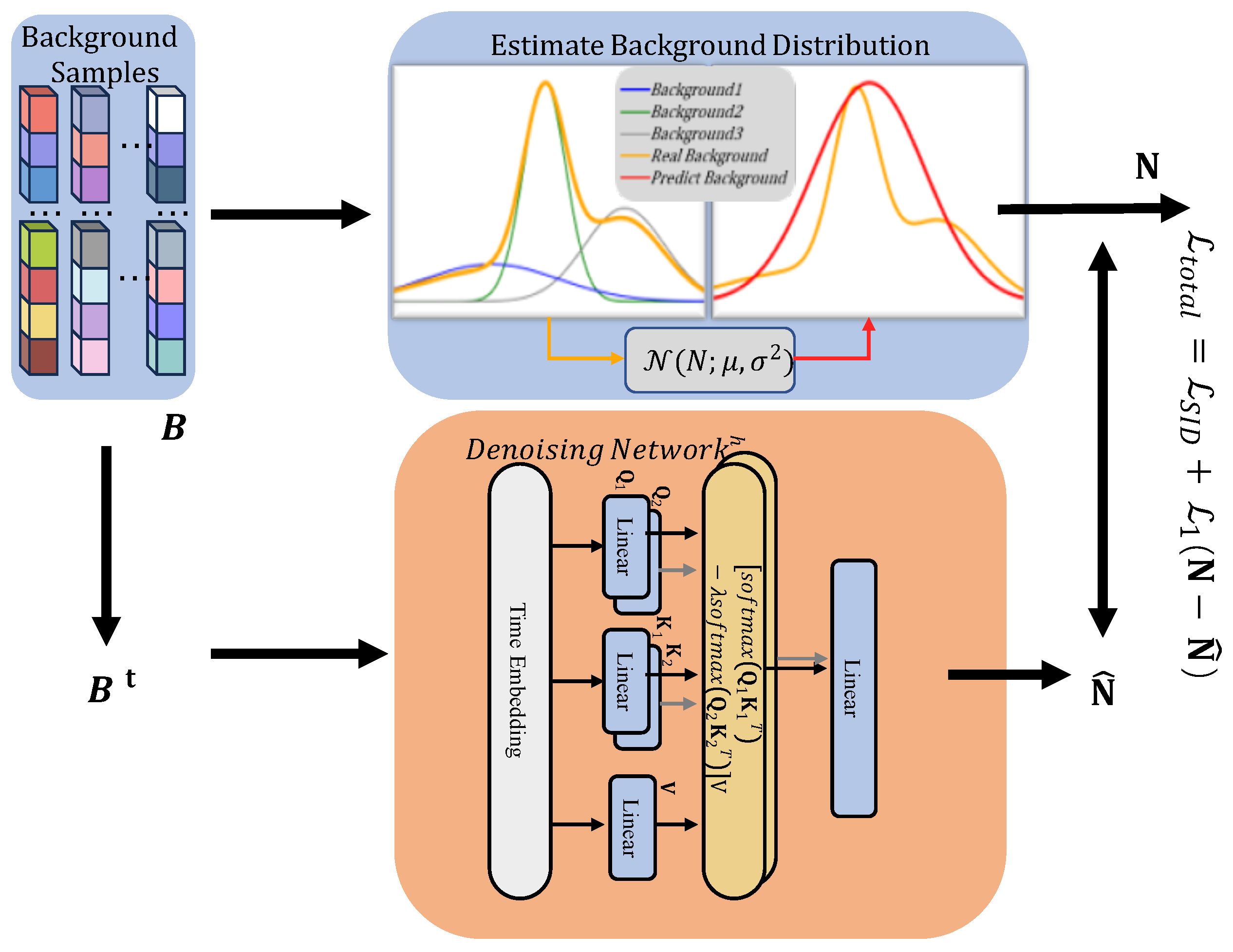
• In order to enhance the learning of hyperspectral information by Diffusion, a SID-based Diffusion model is designed to optimize the loss of Diffusion. Compared with the traditional Diffusion, the performance of the algorithm is improved while using prior spectral information.
• To verify the effectiveness of the method in this paper, the results are compared with the most advanced existing algorithms, which show that our model is superior to existing HTD algorithms.

The rest of this paper is organized as follows. Section 2 reviews the necessary knowledge and related works. Section 3 gives a detailed description of the proposed method. Section 4 presents the experimental setup and results on the data set. Section 5 analyses the experiments. Section 6 concludes and summarizes the paper.

2. Related Work

2.1. Notations

In this paper, tensors, matrices, vectors and scalars are denoted by $\mathcal{H}$, $\mathbf{H}$, $\mathbf{h}$, h. For instance, the HSI tensor is represented by $\mathcal{H}\in {\mathbb{R}}^{h\times w\times L}$,where $h,w,L$ correspond to height, width and the number of spectral band respectively. HSI tensor reshapes as two-dimensional matrix $\mathbf{H}\in {\mathbb{R}}^{n\times L}$, where n represents $h\times w$. The prior spectral vector represents $\mathbf{d}\in {\mathbb{R}}^{L\times 1}$.

2.2. Diffusion Models

A generative model generates samples resembling the training data by learning its probability distribution. The model is robust because it continuously learns the characteristics of the data distribution. In general, the generative models can be divided into naive Bayes, hidden Markov models, GANs, VAEs and diffusion models. Diffusion models have advantages over GANs and VAEs, including training stability, strong interpretability, and the ability to generate high-quality results. Therefore, they have become the mainstream approach for generative models. Denoising diffusion probabilistic models (DDPMs) are the most frequently utilized models [49]. The core concept involves generating data through forward and reverse data denoising processes. Both processes are modeled as parametric Markov chains. The forward process, which lacks learnable parameters, converts samples into standard Gaussian noise through iterative noise addition. The reverse process contains learnable parameters, and the image is denoised and gradually restored during the process, usually using a neural network approach. The model is generally a unet-based model. DDPMs have strong feature generation capabilities and are currently widely used in HSI denoising [50], HSI restoration [51], HSI classification [52], anomaly detection [53] and other tasks, but are rarely involved in the field of HTD. In HTD applications, DDPMs enhance spectral differences between the target and background, facilitating their separation.

2.3. Spectral Information Divergence

In this section, we introduce SID that is used in Section 3. SID is a critical parameter for measuring spectral correlation. It quantifies the spectral similarity of the target to other pixels using Kullback-Leibler (KL) divergence. Supposed $\mathbf{x}=(x_1,x_2,\dots ,x_L)$ is target pixel, $\mathbf{y}=(y_1,y_2,\dots ,y_L)$ represent the other pixel, and L is the number of bands. The probability vector of pixel $\mathbf{x}$ is given by $\mathbf{p}=(p_1,p_2,\dots ,p_L)$, and the probability vector $\mathbf{y}$ of pixel is given by $\mathbf{q}=(q_1,q_2,\dots ,q_L)$, where $p_i={\displaystyle \frac{x_i}{{\sum }_{i=1}^L{x}_i}}$, $q_i={\displaystyle \frac{y_i}{{\sum }_{i=1}^L{y}_i}}$. According to the definition of KL divergence, the relative entropy of the target pixel $\mathbf{x}$ with respect to pixel $\mathbf{y}$ is expressed as:

$$S(\mathbf{x}\parallel \mathbf{y})=\sum _{i=1}^L{q}_{i}log{\displaystyle \frac{q_i}{p_i}}$$

(1)

where $S(·)$ represents KL divergence.The SID is composed of two directions of relative entropy, given by:

$$SID(\mathbf{x}\parallel \mathbf{y})=S(\mathbf{x}\parallel \mathbf{y})+S(\mathbf{y}\parallel \mathbf{x})$$

(2)

Using this method, SID accounts for the bi-directional spectral differences between two pixels, effectively capturing the spectral information between them.

3. Proposed Method

This paper presents a novel HTD framework based on Diffusion joint spectral information divergence constraints. In this paper, the SID idea is integrated with Diffusion to propose a model for better representation of the background. As illustrated in Figure 1, the proposed deep learning method, based on diffusion constraints based on SID, comprises two primary modules: background learning and target comparison detection.

3.1. Double-Branch Adaptive Coarse Detection (DBACD)

The limited availability of target spectra presents a significant challenge for deep network training. Conversely, the abundance of background samples in HSI offers new opportunities for target detection by leveraging the differences between background samples and targets. By reconstructing diverse background samples, the model effectively learns the background distribution characteristics, while the reconstructed target remains significantly different from the background samples. However, previous studies often use a fixed threshold to initially select background samples, which lacks adaptability to dataset distributions, performs poorly across different datasets, and demonstrates limited robustness. In this regard, this paper proposes a Double-Branch Adaptive Coarse Detection method, which can better divide the background samples and target samples. As shown in Figure 2, the comparison between the proposed method and the traditional coarse detection is shown. Inspired by integrated learning, this paper combines two coarse detection algorithms CEM and MF adaptively determines the threshold for separating background and target samples based on the relationship between the mean and variance of the coarse detection results.

Given the input hyperspectral matrix as $\mathcal{H}\in {\mathbb{R}}^{h\times w\times L}$ and a prior spectral information as $\mathbf{d}\in {\mathbb{R}}^{L\times 1}$, the output value of the CEM is

$${\mathbf{D}}_{\mathbf{CEM}}={\mathit{w}}^T\mathcal{H}={\displaystyle \frac{{\mathbf{d}}^T{\mathbf{R}}^{-1}}{\mathbf{d}{\mathbf{R}}^{-\mathbf{1}}{\mathbf{d}}^T}}\mathcal{H}$$

(3)

where $\mathbf{R}=(1/n\mathcal{H}{\mathcal{H}}^T)$ is the inter-correlation tensor and ${\mathcal{D}}_{CEM}\in {\mathbb{R}}^{h\times w\times 1}$. And the tensor ${\mathcal{D}}_{CEM}\in {\mathbb{R}}^{h\times w\times 1}$ unfolds as matrix ${\mathbf{D}}_{CEM}\in {\mathbb{R}}^{h\times w}$. CEM minimizes the filter capacity under predefined conditions by employing a FIR linear filter design.

The Match Filter (MF) [54] method mainly models the background variation by using the mean vector ${\mu }_{\mathbf{MF}}$ and covariance matrix ${\mathsf{\Sigma }}_{\mathbf{MF}}$. The output value of the MF, ${\mathrm{D}}_{\mathbf{MF}}\in {\mathbb{R}}^{h\times w}$ is:

$${\mathbf{D}}_{MF}={\displaystyle \frac{{\left(\mathbf{d}-{\mu }_{MF}\right)}^{\mathbf{T}}{\mathsf{\Sigma }}_{MF}^{-1}\left(\mathbf{H}-{\mu }_{MF}\right)}{{\left(\mathbf{d}-{\mu }_{MF}\right)}^{\mathbf{T}}{\mathsf{\Sigma }}_{MF}^{-1}\left(\mathbf{d}-{\mu }_{MF}\right)}}$$

(4)

These two methods have their own advantages and disadvantages, and we adopt the idea of integrated learning here, so that ${\mathbf{D}}_{CEM}$ and ${\mathbf{D}}_{MF}$ are jointly coarse detected in the second order. The values of pixels that are similar to the a prior spectra are highlighted by the coarse detection. However, traditional methods typically use a fixed threshold for binarization, often leading to the misclassification of numerous background samples and insufficient learning of background characteristics. This paper adopts a method to adaptively determine the threshold value based on the mean and standard deviation of the image. The threshold $th$ is defined as $th={\mu }_1+3\times {\sigma }_1$, where ${\mu }_1$ represents the mean of coarse detection map and ${\sigma }_1$ denotes the standard deviation of the coarse detection map. The coarse detection maps processed through CEM and MF are fused using the coarse detection fusion factor $\iota$, The fusion result is expressed as:

$$\widehat{\mathbf{D}}=\iota \times {\mathbf{D}}_{CEM}+(1-\iota )\times {\mathbf{D}}_{MF}$$

(5)

where $\widehat{\mathbf{D}}$ represents the fused coarse detection map, serving as a crucial component in subsequent target detection processes.

After binarizing the images generated by the two coarse detections, the target and background values converge to 1 and 0, respectively. The threshold, derived from the statistical properties of the image, significantly reduces the likelihood of background misclassification. Following binarization, the intersection of ${\mathbf{D}}_{CEM}$ and ${\mathbf{D}}_{MF}$ produces the binarized map $\mathbf{D}$. By binarizing the map $\mathbf{D}$, the set of background samples $\mathcal{B}$ is identified as shown in Equation (6):

$$\mathcal{B}(\mathrm{i},\mathrm{j},:)=\left\{\begin{array}{cc}0,& \mathbf{D}(\mathrm{i},\mathrm{j})=1\\ \mathcal{H}(\mathrm{i},\mathrm{j},:),& \mathrm{otherwise}\end{array}\right.$$

(6)

where $\mathcal{H}(\mathrm{i},\mathrm{j})$ represents the spectral vector at position $(\mathrm{i},\mathrm{j})$. This approach enables the effective construction of training background samples using the a prior spectra $\mathbf{d}$. We use 75% of the samples for training. Comparative experiments will be conducted in Section 5 to validate the effectiveness of the proposed method.

3.2. Background Learning Based on Diffusion Model

This paper builds on the diffusion model in the BSDM proposed by Ma et al. [53], using a Gaussian distribution $\mathbf{N}\sim \mathcal{N}\left(\mu ,{\sigma }^2\right)$, with the same mean and variance as the input HSI as the pseudo background noise, where $\mu$ is the mean of the background samples and $\sigma$ is the standard deviation of the background samples. Figure 3 illustrates the schematic of the forward noise addition process and the denoising network in the diffusion model.

The zero-moment data $b_0$ is sampled from the background data distribution $q\left(x\right)$, i.e., $b_0\sim q\left(x\right)$. The forward diffusion process involves the gradual addition of T noises to $b_0$, where ${ϵ}_0,\dots ,{ϵ}_{t-2},{ϵ}_{t-1}$ all follow a Gaussian distribution $\mathbf{N}\sim \mathcal{N}\left(\mu ,{\sigma }^2\right)$. This entire process is represented mathematically in Equation (7):

$$\begin{array}{c}q\left(b_t\mid b_{t-1}\right)=\mathcal{N}\left(b_t;\sqrt{1-{\beta }_t}{b}_{t-1}+\mu \sqrt{{\beta }_t},{\sigma }^2{\beta }_t\mathbf{I}\right)\\ \mathrm{s}.\mathrm{t}.,{\beta }_t={\displaystyle \frac{\lambda t}{T}}\end{array}$$

(7)

where $b_t$ represents the background sample after t-step diffusion, ${\beta }_t$ represents the noise intensity, $\lambda$ is a hyperparameter controlling ${\beta }_t$, and and $\mathbf{I}$ is the identity matrix. The forward process can be regarded as a Markov process since each moment t is only related to the $t-1$ moment, so the relationship between the t moment and the initial moment can be recursively introduced as shown in Equation (8):

$$q\left(b_{1:T}\mid b_0\right)=\prod _{t=1}^{T}q\left(b_t\mid b_{t-1}\right)$$

(8)

To simplify the calculation, this paper uses the reparameterization technique in DDPM and defines $\sqrt{{\alpha }_t}=\sqrt{1-{\beta }_t}$, ${\overline{\alpha }}_t={\prod }_{t=1}^T{\alpha }_i$, so that $b_t$ can be expressed as Equation (9):

$$\begin{array}{cc}\hfill b_t& =\sqrt{{\alpha }_t}{b}_{t-1}+\sqrt{1-{\alpha }_t}{ϵ}_{t-1}\hfill \\ \hfill & =\sqrt{{\alpha }_t{\alpha }_{t-1}}{b}_{t-2}+\sqrt{1-{\alpha }_t{\alpha }_{t-1}}{\overline{ϵ}}_{t-2}\hfill \end{array}$$

(9)

Since ${ϵ}_{t-1}$ and ${ϵ}_{t-2}$ both follow a Gaussian distribution, they can be combined based on Gaussian properties, with $\overline{ϵ}$ representing the resulting distribution. Equation (10) is derived through recursion.

$$\begin{array}{c}{b}_t=\sqrt{{\overline{\alpha }}_t}{b}_0+{\theta }_t\overline{ϵ}\\ \mathrm{s}.\mathrm{t}.,{\theta }_tϵ\sim \mathcal{N}\left(\mu {\theta }_t,\left(1-{\overline{\alpha }}_t\right){\sigma }^2\right)\end{array}$$

(10)

$\overline{ϵ}$ represents a Gaussian function comprising multiple moments, and ${\theta }_t={\sum }_{k=0}^{t-1}\sqrt{{\displaystyle \frac{{\overline{\alpha }}_t{\alpha }_{t-k}}{{\overline{\alpha }}_{t-k}}}}$. Substituting this into Equation (8) results in Equation (11):

$$q\left(b_t\mid b_{t-1}\right)=\mathcal{N}\left(b_t;\sqrt{{\overline{\alpha }}_t}{b}_{t-1}+\mu {\theta }_t,\left(1-{\overline{\alpha }}_t\right){\sigma }^2\mathbf{I}\right)$$

(11)

The above describes the forward diffusion process of the diffusion model, which obtains the distribution of background samples at T moments. This process is expressed in Equation (12):

$${\mathbf{B}}^t=\mathbf{B}{\oplus }_t\mathbf{N}=\sqrt{{\overline{\alpha }}_t}\mathbf{B}+{\theta }_t\mathbf{N}$$

(12)

The inverse process of the diffusion model is typically denoised using a deep neural network with the structure of the denoising network illustrated in Figure 3. The spectral vector in ${\mathbf{B}}^t$ serves as the input, while the estimated noise ${\mathit{n}}^i$ at the t-th step is the output, as expressed in Equation (13):

$${\mathit{n}}^i=f\left({\mathbf{B}}^t;\gamma \right)$$

(13)

where f represents the deep learning network and $\gamma$ denotes its parameters. The network f primarily comprises a temporal embedding layer and a differential Transformer. This paper initially adopts the same temporal embedding method as DDPM.

$$\begin{array}{c}\widehat{\mathbf{t}}={Emb}_{\mathrm{t}}\left(\mathrm{t};{\gamma }_{\mathrm{te}}\right),\\ \mathrm{s}.\mathrm{t}.,{\gamma }_{\mathrm{te}}\in \gamma \end{array}$$

(14)

where ${\mathrm{Emb}}_t\left(.;{\gamma }_{te}\right)$ denotes the temporal embedding function network and ${\gamma }_{te}$ represents its parameters.

$$\widetilde{{\mathbf{B}}^t}=g\left({\mathbf{B}}^t,{\gamma }_{\mathrm{linear}}\right)+\widehat{\mathbf{t}}$$

(15)

where $g\left(.;{\gamma }_{linear}\right)$ is the linear transformation layer, with ${\gamma }_{linear}$ as its parameter.

This paper employs a differential transformer-based network for the denoising model [55]. Transformer models often allocate excessive attention to task-irrelevant contextual information, leading to an overemphasis on non-critical parts. The differential attention mechanism mitigates this issue by removing attentional noise and directing the model’s focus toward crucial information. This approach is conceptually analogous to differential amplifiers in electrical engineering. For a given input background sample $\tilde{\mathbf{B}}\in {\mathbb{R}}^{(h\times w)\times L}$, it is first projected onto queries, keys, and values: ${\mathbf{Q}}_1,{\mathbf{Q}}_2,{\mathbf{K}}_1,{\mathbf{K}}_2\in {\mathbb{R}}^{(h\times w)\times L}$ and $\mathbf{V}\in {\mathbb{R}}^{(2\times h\times w)\times L}$. The differential attention $Diff(·)$ is then calculated as follows:

$$\begin{array}{c}\left[{\mathbf{Q}}_1;{\mathbf{Q}}_2\right]=\tilde{\mathbf{B}}{\mathbf{W}}^Q,\left[{\mathbf{K}}_1;{\mathbf{K}}_2\right]=\tilde{\mathbf{B}}{\mathbf{W}}^K,V=\tilde{\mathbf{B}}{\mathbf{W}}^V\\ Diff(\tilde{\mathbf{B}})=(softmax({\displaystyle \frac{{\mathbf{Q}}_1{\mathbf{K}}_1^T}{\sqrt{d}}})-\lambda softmax({\displaystyle \frac{{\mathbf{Q}}_2{\mathbf{K}}_2^T}{\sqrt{d}}}))\mathbf{V}\end{array}$$

(16)

where ${\mathbf{W}}^Q,{\mathbf{W}}^K,{\mathbf{W}}^V\in {\mathbb{R}}^{(2\times h\times w)\times L}$, and $\lambda$ is learnable shared parameter, designed as

$$\lambda =exp\left({\lambda }_{{\mathbf{q}}_1}·{\lambda }_{{\mathbf{k}}_1}\right)-exp\left({\lambda }_{{\mathbf{q}}_2}·{\lambda }_{{\mathbf{k}}_2}\right)+{\lambda }_{\mathrm{init}}$$

(17)

where ${\lambda }_{{\mathbf{q}}_1},{\lambda }_{{\mathbf{k}}_1},{\lambda }_{{\mathbf{q}}_2},{\lambda }_{{\mathbf{k}}_2}$ are learnable parameters, while ${\lambda }_{\mathrm{init}}$ serves as a hyperparameter. Additionally, the multi-head attention mechanism employs, ${\mathbf{W}}_i^Q,{\mathbf{W}}_i^K,{\mathbf{W}}_i^V$, where $i\in \left[1,h\right]$. ${\mathbf{W}}^O$ is a learnable projection matrix.

$$\begin{array}{cc}\hfill & {\mathbf{head}}_i=\mathbf{D}\left(\tilde{\mathbf{B}};{\mathbf{W}}_i^Q,{\mathbf{W}}_i^K,{\mathbf{W}}_i^V,\lambda \right)\hfill \\ \hfill & \overline{{\mathbf{head}}_i}=\left(1-{\lambda }_{\mathrm{init}}\right)·\left(\overline{{\mathbf{head}}_i}\right)\hfill \\ \hfill & \mathbf{MultiHead}\left(\tilde{\mathbf{B}}\right)=\mathrm{Concat}\left(\overline{{\mathbf{head}}_i}\cdots ,\overline{{\mathbf{head}}_h}\right){\mathbf{W}}^O\hfill \end{array}$$

(18)

The output $\tilde{n}$ is obtained after a linear layer transformation. The mean squared error loss function ${\mathcal{L}}_1$ used for the diffusion model is

$${\mathcal{L}}_1=\underset{\theta ,\mathbf{t}}{min}\left({∥\mathbf{N}-f\left({\mathbf{B}}^t;\gamma \right)∥}_2\right)$$

(19)

The background samples classified during coarse detection are often misclassified. To improve the reliability of background reconstruction, this paper proposes a SID-based loss function, which serves as a criterion for target suppression during training. It is introduced in Section 2. The SID is calculated as shown in Equation (2), and the average SID value for each sample is represented as ${\mathcal{L}}_{sid}$, as given in Equation (20):

$${\mathcal{L}}_{sid}={\displaystyle \frac{1}{m}}\sum _i^{m}SID\left[i\right]$$

(20)

where m is the number of background samples. Consequently, the total loss function is expressed in Equation (21):

$${\mathcal{L}}_{total}={\mathcal{L}}_1-\delta \times {\mathcal{L}}_{sid}$$

(21)

3.3. Target Detection

The target detection process corresponds to the reverse denoising process in DDPM. Starting from a predefined pseudo-background noise, the trained denoising network iteratively restores all spectral samples in reverse order, from step $t=T$ to $t=0$. The final output spectral samples closely approximate the true data distribution, denoted as $\widehat{\mathcal{H}}$.

Effective target detection is achieved by analyzing the differences in reconstructed spectra between $\widehat{\mathcal{H}}$ and $\mathcal{H}$. In this study, the spectral angle mapper (SAM) function is utilized, as proposed by previous scholars, to evaluate the degree of change in samples before and after reconstruction. For each ${\mathbf{h}}_{(i,j)}$ and ${\widehat{\mathbf{h}}}_{(i,j)}$, the SAD is calculated using the Equation (22):

$$\begin{array}{cc}\hfill {\mathbf{d}}_M^{i,j}& ={cos}^{-1}\left({\displaystyle \frac{{\left({\mathbf{h}}_{(i,j)}\right)}^T{\widehat{\mathbf{h}}}_{(i,j)}}{\left(∥{\mathbf{h}}_{(i,j)}∥\right)\left(∥{\widehat{\mathbf{h}}}_{(i,j)}∥\right)}}\right)\hfill \\ \hfill & ={cos}^{-1}\left({\displaystyle \frac{{\mathbf{h}}_{(i,j)}{\widehat{\mathbf{h}}}_{(i,j)}}{\sqrt{{\left({\widehat{\mathbf{h}}}_{(i,j)}\right)}^T{\widehat{\mathbf{h}}}_{(i,j)}}\sqrt{{\left({\mathbf{h}}_{(i,j)}\right)}^T{\mathbf{h}}_{(i,j)}}}}\right)\hfill \end{array}$$

(22)

where ${\mathbf{h}}_{(\mathbf{i},\mathbf{j})}$ and ${\widehat{\mathbf{h}}}_{(i,j)}$ represent the spectral profiles of the original and reconstructed spectra at various $(i,j)$, respectively, and ${\mathbf{d}}_M^{i,j}$ represents the distance difference map at different $(i,j)$. To obtain detection targets, ${\mathbf{d}}_M^{i,j}$ at each position is multiplied by the detection map $\widehat{\mathbf{D}}$, which is weighted by the two coarse detections. However, hyperspectral data often exhibit special cases like spectral variability, where poor reconstruction accuracy can cause localized degradation in background suppression. To address this issue, a non-linear function is introduced to suppress pixels with smaller response values while preserving those with higher response values. The nonlinear function $f\left(x\right)$ is defined as:

$$f\left(x\right)=\left\{\begin{array}{cc}1-e^{-\beta x},\hfill & x\ge 0\hfill \\ 0,\hfill & x<0\hfill \end{array}\right.$$

(23)

where $\beta$ is a parameter that determines the background suppression capability. Each detected pixel ${\mathbf{d}}_M^{i,j}$ is multiplied pixel-wise with the weighted detection map $\widehat{D}$ after being processed through the non-linear variation, as defined by the following Equation (24):

$${\widehat{\mathbf{d}}}_M^{i,j}={\mathbf{d}}_M^{i,j}\odot f\left({\widehat{\mathbf{D}}}_{(i,j)}\right)$$

(24)

By this method, the final result is the detection map $\mathbf{R}\in {\mathbb{R}}^{h\times w}$. The overall performance of the HSI is significantly improved, demonstrating substantial enhancement across different datasets. Algorithm 1 summarizes the pseudocode flow of the SID-DN model that we proposed.

Algorithm 1 SID-DN for HSI Target Detection

Require: HSI tensor $\mathcal{X}$, prior target spectrum $\mathbf{d}$ 1: Compute a coarse detection result $\widehat{\mathbf{D}}$ from input $\mathcal{B}$ by (5) 2: Construct the background training set $X_B$ from binarized map $\mathbf{D}$ and input $\mathcal{X}$ by (6) 3: for each epoch do 4:     Minimize the loss function ${\mathcal{L}}_{total}$ in (21) 5: end for 6: Reconstruct $\widehat{\mathcal{H}}$ with the trained model. 7: Compute the spectral distance map ${\mathbf{d}}_M$ by (22) 8: Compute $\mathbf{R}$ from $\widehat{\mathbf{D}}$ and ${\mathbf{d}}_M$ by (23) and (24) Ensure: Target map $\mathbf{R}$

4. Results

This section begins with basic information about the test dataset, followed by the parameter and environment settings for both the proposed and state-of-the-art algorithms. Finally, the two algorithms are compared using objective and subjective metrics.

4.1. Description of Experimental Datasets

In this experiment, three real HTD datasets are selected to validate the proposed algorithm: the Gulfport dataset (part of the ABU dataset), the Los Angeles dataset, and the San Diego dataset. Their basic information is summarized in

Table 1. Basic information on Los Angeles, Gulport and San Diego.

Dataset	Los Angeles	Gulport	San Diego
Sensor	AVRIS	AVRIS	AVRIS
Spatial resolution (m)	7.1	3.4	7.5
Spatial Size	100 × 100	100 × 100	100 × 100
Number of bands	205	191	189
Spectral range ($\mathsf{\mu }$m)	0.4∼2.5	0.4∼2.5	0.37∼2.51
Spectral resolution (nm)	10	10	10
Number of Target (Pixels)	87	60	57

. The Gulfport and Los Angeles datasets are derived from the ABU dataset collected by Kang et al. [56], with aircraft as the detection objects. Low signal-to-noise spectra and spectra impacted by water vapor interference, including bands 1–6, 33–35, 97, 107–113, 153–166 and 221–224, are eliminated for the San Diego dataset. The remaining 189-dimensional spectra are used for experiments, with aircraft as the detection objects. The image sizes of the three datasets shown in Table 1 represent cropped dimensions.

4.2. Evaluation Metrics

To comprehensively evaluate HTD performance, this paper uses the 2-D and 3-D Receiver Operating Characteristic Curves (ROC) and the target-background separation map as objective evaluation metrics.

The ROC curve illustrates the relationship between the detection rate $P_D\left(\tau \right)$ and the false alarm rate $P_F\left(\tau \right)$ as the classification threshold $\tau$ varies. The corresponding formula is provided in Equations (25) and (26).

$$P_D\left(\tau \right)={\displaystyle \frac{TP}{TP+FN}}$$

(25)

$$P_F\left(\tau \right)={\displaystyle \frac{FP}{FP+TN}}$$

(26)

The detection rate $P_D\left(\tau \right)$ is defined as the proportion of positive cases correctly detected at a given threshold $\tau$, as described in Equation (25). The false alarm rate $P_F\left(\tau \right)$ is the proportion of incorrectly detected positive cases relative to all negative cases at threshold $\tau$, as shown in Equation (26). An ideal ROC curve approaches the upper left corner (0,1), indicating a high detection rate and a low false alarm rate.

By varying the threshold $\tau$, 2D ROC curves $(\tau ,P_D\left(\tau \right))$ and $(\tau ,P_F\left(\tau \right))$ can be plotted. A faster rise in the 2D ROC curves $(\tau ,P_D\left(\tau \right))$ indicates a higher detection rate, and a faster decline in the 2D ROC curves $(\tau ,P_D\left(\tau \right))$ indicates a lower false alarm rate.

The Area Under the Curve (AUC) represents the area enclosed by the ROC curve and $P_D\left(\tau \right)$, as defined in Equation (27). A larger AUC value indicates a higher detection rate for the model.

$$\mathrm{AUC}={\int }_0^1{P}_D\left(\tau \right)d{P}_F\left(\tau \right)$$

(27)

To further evaluate the target detection performance of the model, Chang et al. [57] proposed a 3D ROC curve detection method. The 3D ROC curve includes five key metrics: ${\mathrm{AUC}}_{\left(P_F,P_D\right)}$, ${\mathrm{AUC}}_{\left(\tau ,P_D\left(\tau \right)\right)}$${\mathrm{AUC}}_{\left(\tau ,P_F\left(\tau \right)\right)}$, ${\mathrm{AUC}}_{BS}$, ${\mathrm{AUC}}_{SNPR}$. Calculated using Equations (28) and (29):

$${\mathrm{AUC}}_{BS}={\mathrm{AUC}}_{\left(P_F,P_D\right)}-{\mathrm{AUC}}_{\left(\tau ,P_F\left(\tau \right)\right)}$$

(28)

$${\mathrm{AUC}}_{SNPR}={\displaystyle \frac{{\mathrm{AUC}}_{\left(\tau ,P_D\right)}}{{\mathrm{AUC}}_{\left(\tau ,P_F\left(\tau \right)\right)}}}$$

(29)

The value of ${\mathrm{AUC}}_{\left(P_D,P_F\right)}$ is interpreted the same way as AUC: a larger value indicates better detection algorithm performance, with an optimal value of 1. ${\mathrm{AUC}}_{\left(P_D,P_F\right)}$ represents the overall performance of the algorithm and is the most important metric. However, ${\mathrm{AUC}}_{\left(\tau ,P_F\left(\tau \right)\right)}$ is interpreted differently: a smaller value signifies better performance, with the optimal value being 0. a smaller ${\mathrm{AUC}}_{\left(\tau ,P_F\left(\tau \right)\right)}$ value reflects a lower false alarm rate and better background suppression. ${\mathrm{AUC}}_{BS}$ is a composite indicator calculated by weighting and summing the two AUC metrics. Consequently, a larger ${\mathrm{AUC}}_{BS}$ value indicates better detection algorithm performance, with the optimal value being 1. ${\mathrm{AUC}}_{SNPR}$ is inspired by the concept of Signal-to-Noise Ratio (SNR), where ${\mathrm{AUC}}_{\left(P_F,P_D\right)}$ represents the signal and ${\mathrm{AUC}}_{\left(\tau ,P_F\left(\tau \right)\right)}$ represents the noise. A larger ${\mathrm{AUC}}_{SNPR}$ value indicates better performance of the detection algorithm, with the optimal value being $+\infty$. The 3D ROC curve provides a three-dimensional visualization, allowing for intuitive assessment of the impact of threshold $\tau$ on the detection rate $P_D\left(\tau \right)$ and the false alarm rate $P_F\left(\tau \right)$.

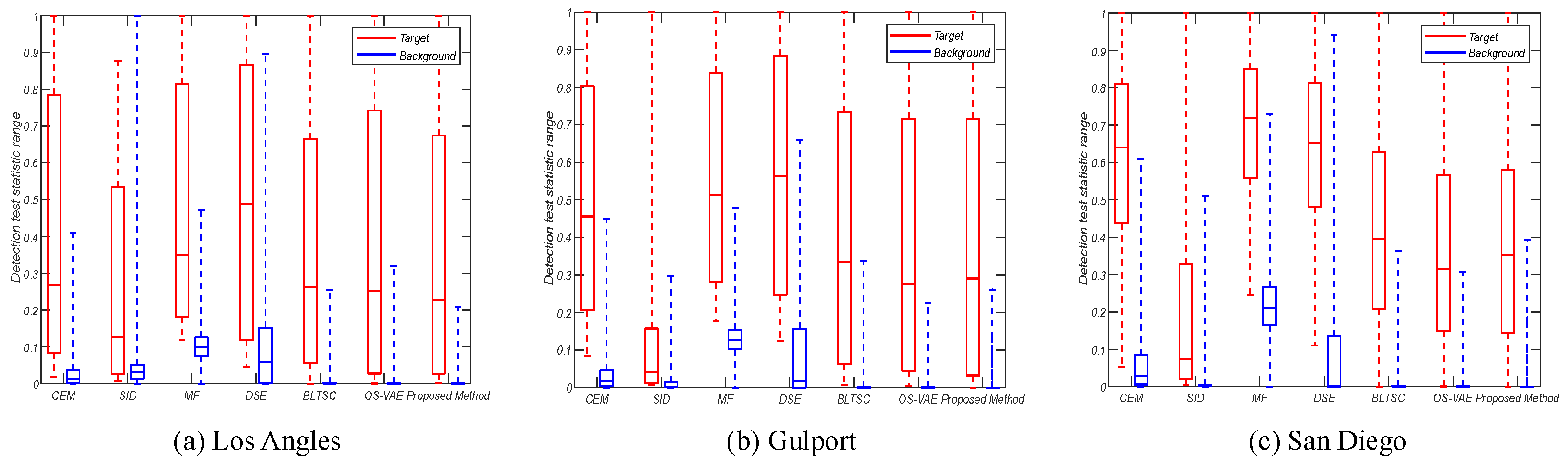
The target-background separation map, using the Box-Whisker method, analyzes the separation between target and background. There are two main criteria for evaluation. The first criterion is whether there is any overlap between the target box and the background box. If overlap exists, it indicates that the target and background are mixed during the detection process, making it difficult to distinguish them. The second criterion is based on the area of the background box. The upper and lower bounds of the box represent the 75th and 25th percentiles of the data, respectively. A smaller box indicates that the data are more concentrated, and background suppression is more effective.

4.3. Experimental Environment and Contrasting Models

The hardware used in this experiment includes an i7-12700K CPU, NVIDIA GTX 3090Ti 24 GB graphics card, and 128 GB RAM. The software environment comprises Windows Subsystem for Linux (WSL), PyTorch 1.11.0, and Python 3.8.

To evaluate the efficiency of the algorithms proposed in this paper, traditional target detection methods such as CEM [14], SID [18], MF [54] and sparse representation method as DSE [32], as well as deep learning models like BLTSC [41] and OS-VAE [45], were selected for comparison. All comparison algorithms were configured with the optimal parameters specified in the respective papers.

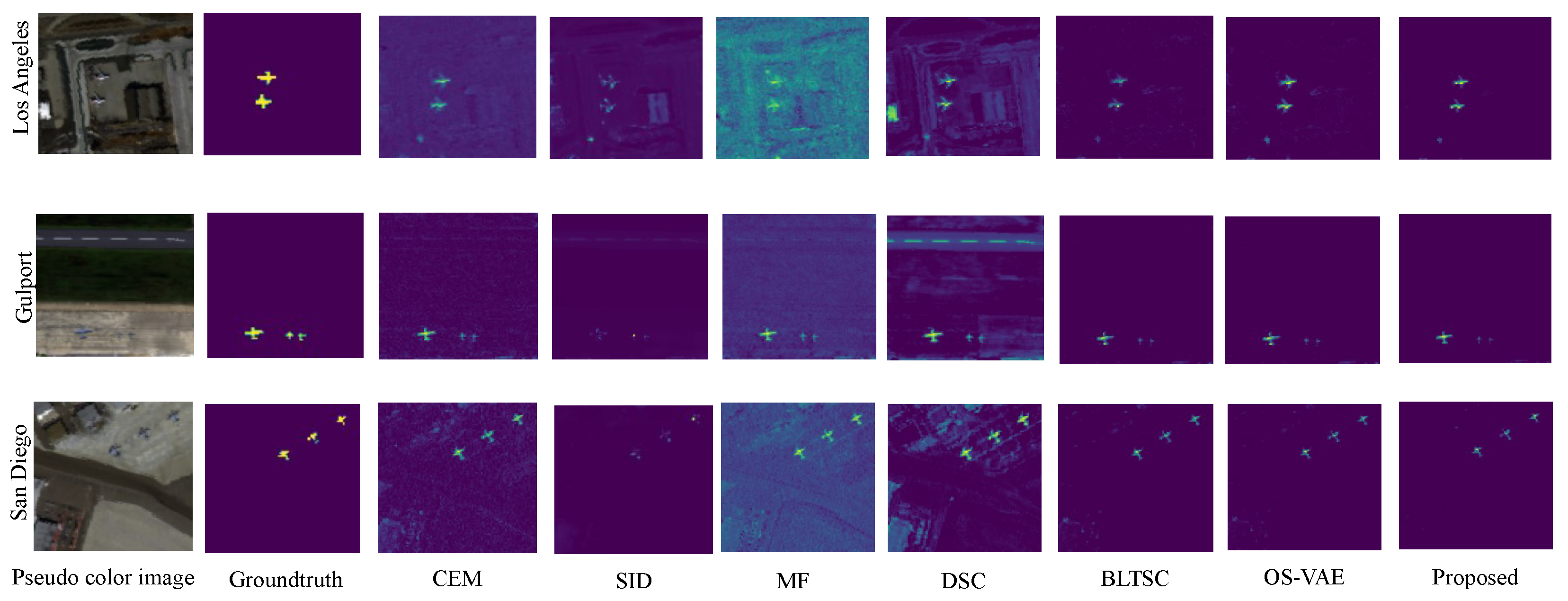
4.4. Comparative Results on HSI Target Detection

Figure 4 visualizes the detection maps generated by all comparison methods and the proposed method on three real datasets. The results demonstrate that the SID-DN method outperforms the other methods in both target detection and background suppression. Classical detection techniques like MF, CEM and SID exhibit high accuracy in target detection but struggle to filter extensive background information, resulting in insufficient background suppression. Likewise, the DSC method performs poorly in handling complex spectral scenarios, leading to increased false alarm targets. The SID-DN method excels in background suppression, effectively suppressing target-independent background information compared to recently proposed methods such as BLTSC and OS-VAE. BLTSC and OS-VAE, which are generative deep learning models that incorporate background generation representation, slightly lag behind the SID-DN algorithm in background suppression. This confirms the effectiveness of incorporating SID concepts into network design. Furthermore, using SID-DN, particularly on the Los Angeles dataset, the distinction between the target and background is highly evident, demonstrating that the reconstructed background closely resembles the real situation. Additionally, this paper enhances the coarse detection algorithm, significantly reducing target interference in the learning of background samples. The incorporation of SID concepts effectively eliminates potential bad samples, enabling accurate reconstruction of background samples. In summary, the SID-DN method proposed in this paper demonstrates competitive advantages in both target detection and background suppression.

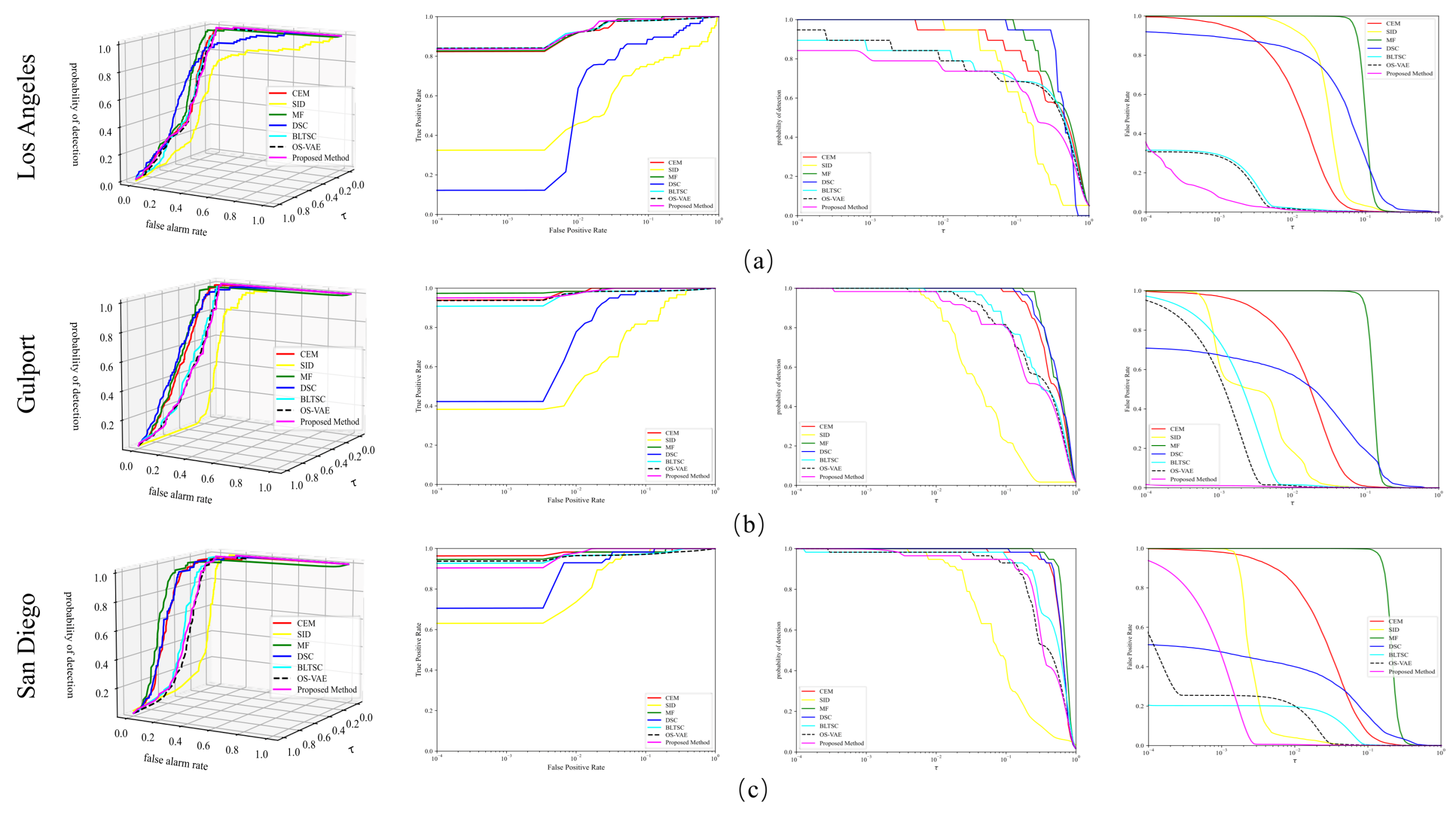
Figure 5 presents the 3D ROC curves corresponding to the above detection results. Compared to the other algorithms, SID-DN achieves results closer to the upper left corner of the test dataset in terms of the ${\mathrm{AUC}}_{(P_D,P_F)}$ metric. However, SID-DN performs slightly worse than DSE and MF in ${\mathrm{AUC}}_{\left(P_F,P_D\right)}$. This is because SID-DN focuses on learning background features through reconstruction, but the target spectral reconstruction remains suboptimal, resulting in weaker target intensity in detection and impacting this metric. Conversely, SID-DN is closer to the bottom right corner in the ${\mathrm{AUC}}_{\left(\tau ,P_F\left(\tau \right)\right)}$ curve, indicating its superior background suppression capabilities compared to other methods. This observation highlights the importance of considering multiple metrics in evaluating algorithm performance. In summary, SID-DN achieves a highly advantageous average optimal detection rate across all three datasets.

While ROC curves visually represent the results, accurately assessing them can be challenging due to overlapping curves among the compared methods. Thus, the five AUC metrics across the three datasets are analyzed in detail in

Table 2. Performance comparison of different methods across various AUC metrics on the Los Angeles dataset.

Method	${\mathbf{AUC}}_{({\mathit{P}}_{\mathit{F}},{\mathit{P}}_{\mathit{D}})}$	${\mathbf{AUC}}_{(\mathit{\tau },{\mathit{P}}_{\mathit{D}})}$	${\mathbf{AUC}}_{(\mathit{\tau },{\mathit{P}}_{\mathit{F}})}$	${\mathbf{AUC}}_{\mathit{BS}}$	${\mathbf{AUC}}_{\mathit{SNPR}}$	Running Time
CEM [14]	0.9929	0.3618	0.0176	0.9753	20.49	0.14
SID [18]	0.8499	0.2015	0.0361	0.8138	5.572	0.09
MF [54]	0.9958	0.4306	0.1015	0.8943	4.24	0.08
DSE [32]	0.9470	0.4725	0.0762	0.8708	6.19	21.92
BLTSC [41]	0.9944	0.3353	0.0011	0.9933	297.95	2.83
OS-VAE [45]	0.9943	0.3311	0.0010	0.9933	318.38	2.69
Proposed	0.9967	0.3146	0.0007	0.9960	410.53	0.37

Note: The best results are highlighted in bold.

,

Table 3. Performance comparison of different methods across various AUC metrics on the Gulfport dataset.

Method	${\mathbf{AUC}}_{({\mathit{P}}_{\mathit{F}},{\mathit{P}}_{\mathit{D}})}$	${\mathbf{AUC}}_{(\mathit{\tau },{\mathit{P}}_{\mathit{D}})}$	${\mathbf{AUC}}_{(\mathit{\tau },{\mathit{P}}_{\mathit{F}})}$	${\mathbf{AUC}}_{\mathit{BS}}$	${\mathbf{AUC}}_{\mathit{SNPR}}$	Running Time
CEM [14]	0.9993	0.5005	0.0225	0.9768	22.18	0.007
SID [18]	0.9489	0.0800	0.0050	0.9439	13.43	0.09
MF [54]	0.9992	0.5435	0.1286	0.8706	4.22	0.023
DSE [32]	0.9900	0.5670	0.0525	0.9375	10.78	18.78
BLTSC [41]	0.9990	0.3671	0.0008	0.9982	445.18	2.57
OS-VAE [45]	0.9992	0.3381	0.0005	0.9987	645.46	2.7
Proposed	0.9994	0.3547	0.0002	0.9992	1742.73	0.47

Note: The best results are highlighted in bold.

and

Table 4. Performance comparison of different methods across various AUC metrics on San Diego dataset.

Method	${\mathbf{AUC}}_{({\mathit{P}}_{\mathit{F}},{\mathit{P}}_{\mathit{D}})}$	${\mathbf{AUC}}_{(\mathit{\tau },{\mathit{P}}_{\mathit{D}})}$	${\mathbf{AUC}}_{(\mathit{\tau },{\mathit{P}}_{\mathit{F}})}$	${\mathbf{AUC}}_{\mathit{BS}}$	${\mathbf{AUC}}_{\mathit{SNPR}}$	Running Time
CEM [14]	0.9955	0.6265	0.0395	0.9560	15.82	0.007
SID [18]	0.9916	0.1588	0.0035	0.9881	44.27	0.083
MF [54]	0.9962	0.7093	0.2140	0.7822	3.30	0.024
DSE [32]	0.9941	0.6447	0.0455	0.9486	14.152	71.08
BLTSC [41]	0.9961	0.4167	0.0019	0.9942	215.57	2.54
OS-VAE [45]	0.9951	0.3454	0.0013	0.9938	253.7	2.7
Proposed	0.9969	0.3765	0.0002	0.9967	1409.55	0.35

Note: The best results are highlighted in bold.

.

In Table 2, Table 3 and Table 4, the best results are highlighted in bold. The proposed method achieves the best performance on the most critical metric, ${\mathrm{AUC}}_{(P_D,P_F)}$ demonstrating the superiority of the algorithm. ${\mathrm{AUC}}_{\left(\tau ,P_D\left(\tau \right)\right)}$ typically shows an inverse trend with ${\mathrm{AUC}}_{\left(\tau ,P_F\left(\tau \right)\right)}$, where a large value of ${\mathrm{AUC}}_{\left(\tau ,P_D\left(\tau \right)\right)}$ corresponds to a small value of ${\mathrm{AUC}}_{\left(\tau ,P_F\left(\tau \right)\right)}$, or vice versa. Due to limitations in background reconstruction, SID-DN does not achieve the best results in ${\mathrm{AUC}}_{\left(\tau ,P_D\left(\tau \right)\right)}$. However, it achieves the highest average performance in ${\mathrm{AUC}}_{\left(\tau ,P_F\left(\tau \right)\right)}$, ${\mathrm{AUC}}_{BS}$ and ${\mathrm{AUC}}_{SNPR}$, strongly indicating its effectiveness in suppressing the complex backgrounds of HSI. In conclusion, the AUC scores from the comprehensive performance analysis highlight the sophistication and robustness of the proposed SID-DN algorithm.

This paper further evaluates the target-background separation performance of SID-DN compared to other methods across three datasets. As shown in Figure 6, SID-DN achieves superior target-to-background separation ratios, better separation between target and background, and smaller overlapping regions across all datasets. Additionally, SID-DN effectively suppresses background interference, further demonstrating the algorithm’s effectiveness.

In conclusion, the proposed SID-DN method delivers outstanding performance in both subjective and objective metrics, including detection maps and 3D-ROC curves, while demonstrating superior target-background separation capability across multiple datasets.

5. Discussion

5.1. Ablation Comparison Experiment

The SID-DN proposed in this paper introduces two key innovations: the Double-Branch Adaptive Coarse Detection and the integration of the SID concept into Diffusion networks. To validate the effectiveness of these two innovations, ablation experiments were conducted on each dataset, with results summarized in

Table 5. An ablation study was conducted on three datasets to evaluate the effectiveness of the proposed method.

Dataset	DBACD	$\mathcal{L}\_\mathit{sid}$	${\mathbf{AUC}}_{({\mathit{P}}_{\mathit{D}},{\mathit{P}}_{\mathit{F}})}$	$\mathbf{AUC}\_(\mathit{\tau },{\mathit{P}}_{\mathit{D}})$	${\mathbf{AUC}}_{(\mathit{\tau },{\mathit{P}}_{\mathit{F}})}$	${\mathbf{AUC}}_{\mathit{BS}}$	${\mathbf{AUC}}_{\mathit{SNPR}}$
Los Angeles	×	×	0.9942	0.3668	0.0028	0.9914	126.77
	✓	×	0.9960	0.3295	0.0007	0.9953	430.21
	✓	✓	0.9965	0.3243	0.0006	0.9959	519.54
Gulfport	×	×	0.9992	0.3668	0.005	0.9942	63.50
	✓	×	0.9993	0.3581	0.0006	0.9987	559.50
	✓	✓	0.9994	0.3282	0.0001	0.9993	1997.28
San Diego	×	×	0.9947	0.3384	0.0049	0.9898	67.89
	✓	×	0.9961	0.3325	0.0022	0.9939	147.81
	✓	✓	0.9969	0.3765	0.0002	0.9967	1409.55

Note: The best results are highlighted in bold.

. In Table 5, the first row of each dataset shows the detection results with a fixed threshold. The second row presents results after applying the Double-Branch Adaptive Coarse Detection, while the third row includes results after applying both the Double-Branch Adaptive Coarse Detection and the incorporation of SID. The results show that the quantitative detection results considering the SID loss outperform the quantitative detection results obtained without considering the SID. This finding highlights the robustness of the Double-Branch Adaptive Coarse Detection and SID loss in enhancing the Diffusion network for reconstructing HSI. By thresholding the adaptive coarse detection and integrating the SID concept into the network, the influence of potential targets on background learning is minimized. This reduces interference from target spectra on background spectra, ensuring a smaller discrepancy between the reconstructed and original background spectra, which enables accurate target-background separation. This work not only introduces novel approaches to the generative coarse detection process but also significantly improves the effectiveness of Diffusion-based generative spectral learning.

5.2. Parametric Analysis

This section discusses key hyperparameters in the SID-DN method, including coarse detection fusion parameters $\iota$, the temporal embedding layer in Diffusion ${\gamma }_{\mathrm{te}}$, regularization parameters for SID $\delta$, and background suppression $\beta$.

Firstly, selecting appropriate coarse detection fusion parameters is crucial for obtaining satisfactory detection result $\iota$, as these parameters significantly influence the distribution of $\widehat{D}$ in Equation (5).

Table 6. Sensitivity analysis of $\iota$ was conducted on three datasets.

$\mathit{\iota }$	0.1	0.2	0.3	0.4	0.5	0.6	0.7	0.8	0.9
Los Angeles	0.9949	0.9954	0.9961	0.9963	0.9965	0.9966	0.9966	0.9967	0.9967
Gulport	0.9991	0.9993	0.9992	0.9993	0.9992	0.9994	0.9992	0.9987	0.9985
San Deigo	0.9956	0.9959	0.9961	0.9969	0.9958	0.9956	0.9952	0.9945	0.9933

Note: The best results are highlighted in bold.

presents the detection results obtained with different coarse detection ratios across all datasets. As observed in Table 6, the Los datasets achieve maximum performance at a coarse detection ratio of 0.8, while the Gulfport reach their maximum at 0.6 and San Diego datasets reach their maximum at 0.4. This indicates that varying coarse detection fusion ratios can combine the strengths of both methods, thereby enhancing detection results.

Secondly, this paper examines the impact of the number of temporal embedding nodes ${\gamma }_{\mathrm{te}}$ on the results. Generally, increasing the number of temporal embedding nodes improves performance; however, an excessive number of nodes can lead to parameter redundancy, ultimately degrading network performance. Therefore, it is important to set a reasonable number of temporal embedding nodes. As shown in

Table 7. Sensitivity analysis of ${\gamma }_{\mathrm{te}}$ was conducted on three datasets.

Dataset	32	64	128	256	512
Los Angeles	0.9964	0.9965	0.9966	0.9967	0.9964
Gulport	0.9993	0.9992	0.9994	0.9988	0.9984
San Deigo	0.9584	0.9677	0.9969	0.9959	0.9861

Note: The best results are highlighted in bold.

, all datasets achieve optimal performance with 128 nodes. Accordingly, we set the number of temporal embedding nodes to 128 in our experiments.

Thirdly, the regularization parameter $\delta$ determines the impact of ${\mathcal{L}}_{sid}$ on the performance of the network algorithm. An appropriate ${\mathcal{L}}_{sid}$ suppresses potential targets, enabling effective background learning and ensuring that the reconstruction results successfully separate the target from the background. However, an excessively large ${\mathcal{L}}_{sid}$ can hinder target reconstruction, reducing performance.

Table 8. Sensitivity analysis of $\delta$ was conducted on three datasets.

Dataset	$1\times {10}^{-4}$	$1\times {10}^{-3}$	$1\times {10}^{-2}$	$1\times {10}^{-1}$	1
Los Angeles	0.9960	0.9960	0.9962	0.9965	0.9964
Gulport	0.9994	0.9994	0.9994	0.9994	0.9993
San Deigo	0.9964	0.9964	0.9963	0.9969	0.9966

Note: The best results are highlighted in bold.

demonstrates that an optimal balance between the two loss functions is achieved at $\delta =0.01$. Consequently, we set $\delta$ to 0.01 in our experiments.

During the background suppression phase, selecting an appropriate parameter $\beta$ effectively suppresses the background while highlighting the target. This parameter primarily reflects the strength of the non-linear suppression function in reducing background interference. As shown in

Table 9. Sensitivity analysis of $\beta$ was conducted on three datasets.

Dataset	4	8	12	16	20
Los Angeles	0.9964	0.9967	0.9962	0.9953	0.9938
Gulport	0.9993	0.9994	0.9993	0.9993	0.9992
San Deigo	0.842	0.9822	0.9907	0.9901	0.9969

Note: The best results are highlighted in bold.

, the background suppression capability increases with a higher beta initially, but then starts to decline. A smaller $\beta$ leads to insufficient background suppression, while an excessively high beta causes the non-linear function to lose its ability to suppress, failing to preserve potential targets. Based on comprehensive experimental analysis, we selected $\beta$ values of 8 for Los Angeles and Gulfport, 12 for San Diego. These values were chosen to achieve optimal performance across the datasets.

To further validate the impact of the diffusion denoising model on hyperspectral target detection, we selected CNN-based Unet network [53] and Vision Transformer [58] as denoising diffusion models, respectively, for comparison with our DiffTransformer. ${AUC}_{(P_D,P_F)}$ is primarily used to measure detection performance accuracy, while Params is used to measure the number of parameters in deep learning models, and FLOPs are used to assess the model’s computational efficiency and speed. As shown in the

Table 10. The performance comparison of different denoising diffusion models three datasets.

Dataset		U-Net	VIT	SID-DN
Los Angeles	Params	1.15 M	0.73 M	0.46 M
	FLOPs	1.1 G	0.75 G	0.47 G
	${AUC}_{(P_D,P_F)}$	0.9960	0.9961	0.9965
Gulport	Params	1.13 M	0.71 M	0.44 M
	FLOPs	1.1G	0.73 G	0.45 G
	${AUC}_{(P_D,P_F)}$	0.9992	0.9992	0.9994
Sandiego	Params	1.13 M	0.83 M	0.43 M
	FLOPs	1.1 G	0.85 G	0.44 G
	${AUC}_{(P_D,P_F)}$	0.9958	0.9954	0.9969

Note: The best results are highlighted in bold.

, our method achieves the best results in terms of ${AUC}_{(P_D,P_F)}$, Params, and FLOPs, demonstrating the effectiveness of the method we employed.

6. Conclusions

This paper studies the challenges in generative HTD. From a theoretical perspective, we analyze the key aspects of generative HTD and address the shortcomings of the original algorithm. From a technical perspective, we propose a novel deep learning model that integrates SID with Diffusion to effectively guide the reconstruction of the generative model, incorporating SID information constraints. The SID loss and Diffusion process are co-optimized to enhance the reconstruction capability of the generative model. Experiments on multiple real HSI datasets demonstrate the effectiveness and robustness of the SID-DN algorithm. The results indicate that the SID-DN algorithm achieves state-of-the-art performance in both background suppression and detection accuracy when compared to existing methods. Specifically, our method provides an improvement of at least 50% in ${AUC}_{SNPR}$. Future work will focus on optimizing the coarse detection process to minimize the influence of hyperparameters and further enhance detection accuracy, improving overall network performance.Furthermore, we plan to explore the potential applications of our proposed algorithm in real-world scenarios, such as military detection and environmental monitoring, as well as attempt multi-modal data fusion with hyperspectral and LiDAR data. Additionally, we aim to investigate target detection in complex scenes using SID-DN in combination with UAV-based hyperspectral imaging systems.

References

1. Hong, D.; Li, C.; Zhang, B.; Yokoya, N.; Benediktsson, J.A.; Chanussot, J. Multimodal artificial intelligence foundation models: Unleashing the power of remote sensing big data in earth observation. Innovation 2024, 2, 100055. [Google Scholar] [CrossRef]
2. Nasrabadi, N.M. Hyperspectral target detection: An overview of current and future challenges. IEEE Signal Process. Mag. 2013, 31, 34–44. [Google Scholar] [CrossRef]
3. Ullah, F.; Ullah, I.; Khan, R.U.; Khan, S.; Khan, K.; Pau, G. Conventional to deep ensemble methods for hyperspectral image classification: A comprehensive survey. IEEE J. Sel. Top. Appl. Earth Obs. Remote Sens. 2024, 17, 3878–3916. [Google Scholar]
4. Lin, S.; Cheng, X.; Zeng, Y.; Huo, Y.; Zhang, M.; Wang, H. Low-rank and sparse representation inspired interpretable network for hyperspectral anomaly detection. IEEE Trans. Instrum. Meas. 2024, 73, 5033116. [Google Scholar]
5. Chen, B.; Liu, L.; Zou, Z.; Shi, Z. Target detection in hyperspectral remote sensing image: Current status and challenges. Remote Sens. 2023, 15, 3223. [Google Scholar] [CrossRef]
6. Cheng, G.; Huang, Y.; Li, X.; Lyu, S.; Xu, Z.; Zhao, H.; Zhao, Q.; Xiang, S. Change detection methods for remote sensing in the last decade: A comprehensive review. Remote Sens. 2024, 16, 2355. [Google Scholar] [CrossRef]
7. Reddy, K.K.; Daduvy, A.; Mohana, R.M.; Assiri, B.; Shuaib, M.; Alam, S.; Sheneamer, A. Enhancing precision agriculture and land cover classification: A self-attention 3D convolutional neural network approach for hyperspectral image analysis. IEEE Access 2024, 12, 125592–125608. [Google Scholar] [CrossRef]
8. Shen, M.; Zhao, W.; Jiang, N.; Liu, L.; Cao, R.; Yang, W.; Zhu, X.; Wang, C.; Chen, X.; Chen, J.; et al. Challenges in remote sensing of vegetation phenology. Innov. Geosci. 2024, 2, 100070. [Google Scholar]
9. Li, Q.; Li, J.; Li, T.; Feng, Y. A Joint Framework for Underwater Hyperspectral Image Restoration and Target Detection with Conditional Diffusion Model. IEEE J. Sel. Top. Appl. Earth Obs. Remote Sens. 2024, 17, 17263–17277. [Google Scholar]
10. Bedini, E. The use of hyperspectral remote sensing for mineral exploration: A review. J. Hyperspectr. Remote Sens. 2017, 7, 189–211. [Google Scholar]
11. Adetutu, A.E.; Bayo, Y.F.; Emmanuel, A.A.; Opeyemi, A.A.A. A Review of Hyperspectral Imaging Analysis Techniques for Onset Crop Disease Detection, Identification and Classification. J. For. Environ. Sci. 2024, 40, 80. [Google Scholar]
12. Kruse, F.A.; Lefkoff, A.B.; Boardman, J.W.; Heidebrecht, K.B.; Shapiro, A.; Barloon, P.; Goetz, A.F. The spectral image processing system (SIPS)—interactive visualization and analysis of imaging spectrometer data. Remote Sens. Environ. 1993, 44, 145–163. [Google Scholar]
13. Fuhrmann, D.R.; Kelly, E.J.; Nitzberg, R. A CFAR adaptive matched filter detector. IEEE Trans. Aerosp. Electron. Syst 1992, 28, 208–216. [Google Scholar]
14. Farrand, W.H.; Harsanyi, J.C. Mapping the distribution of mine tailings in the Coeur d’Alene River Valley, Idaho, through the use of a constrained energy minimization technique. Remote Sens. Environ. 1997, 59, 64–76. [Google Scholar]
15. Du, Q.; Chang, C.I. A signal-decomposed and interference-annihilated approach to hyperspectral target detection. IEEE Trans. Geosci. Remote Sens. 2004, 42, 892–906. [Google Scholar]
16. Chen, Y.; Nasrabadi, N.M.; Tran, T.D. Sparse representation for target detection in hyperspectral imagery. IEEE J. Sel. Top. Signal Process. 2011, 5, 629–640. [Google Scholar]
17. Kraut, S.; Scharf, L.L. The CFAR adaptive subspace detector is a scale-invariant GLRT. IEEE Trans. Signal Process. 1999, 47, 2538–2541. [Google Scholar]
18. Chang, C.I. An information-theoretic approach to spectral variability, similarity, and discrimination for hyperspectral image analysis. IEEE Trans. Inf. Theory 2000, 46, 1927–1932. [Google Scholar]
19. Wang, T.; Du, B.; Zhang, L. An automatic robust iteratively reweighted unstructured detector for hyperspectral imagery. IEEE J. Sel. Top. Appl. Earth Obs. Remote Sens. 2014, 7, 2367–2382. [Google Scholar]
20. Kraut, S.; Scharf, L.L.; McWhorter, L.T. Adaptive subspace detectors. IEEE Trans. Signal Process. 2001, 49, 1–16. [Google Scholar]
21. Kwon, H.; Nasrabadi, N.M. Kernel adaptive subspace detector for hyperspectral imagery. IEEE Geosci. Remote Sens. Lett. 2006, 3, 271–275. [Google Scholar] [CrossRef]
22. Zou, Z.; Shi, Z. Hierarchical suppression method for hyperspectral target detection. IEEE Trans. Geosci. Remote Sens. 2015, 54, 330–342. [Google Scholar] [CrossRef]
23. Zhao, R.; Shi, Z.; Zou, Z.; Zhang, Z. Ensemble-based cascaded constrained energy minimization for hyperspectral target detection. Remote Sens. 2019, 11, 1310. [Google Scholar] [CrossRef]
24. Yang, X.; Zhao, M.; Shi, S.; Chen, J. Deep constrained energy minimization for hyperspectral target detection. IEEE J. Sel. Top. Appl. Earth Obs. Remote Sens. 2022, 15, 8049–8063. [Google Scholar] [CrossRef]
25. Thai, B.; Healey, G. Invariant subpixel material detection in hyperspectral imagery. IEEE Trans. Geosci. Remote Sens. 2002, 40, 599–608. [Google Scholar] [CrossRef]
26. Cheng, T.; Wang, B. Decomposition model with background dictionary learning for hyperspectral target detection. IEEE J. Sel. Top. Appl. Earth Obs. Remote Sens. 2021, 14, 1872–1884. [Google Scholar] [CrossRef]
27. Harsanyi, J.C.; Chang, C.I. Hyperspectral image classification and dimensionality reduction: An orthogonal subspace projection approach. IEEE Trans. Geosci. Remote Sens. 1994, 32, 779–785. [Google Scholar] [CrossRef]
28. Chang, C.I.; Chen, J. Orthogonal subspace projection using data sphering and low-rank and sparse matrix decomposition for hyperspectral target detection. IEEE Trans. Geosci. Remote Sens. 2021, 59, 8704–8722. [Google Scholar] [CrossRef]
29. Li, W.; Du, Q.; Zhang, B. Combined sparse and collaborative representation for hyperspectral target detection. Pattern Recognit. 2015, 48, 3904–3916. [Google Scholar] [CrossRef]
30. Liu, R.; Wu, J.; Zhu, D.; Du, B. Weighted Discriminative Collaborative Competitive Representation with Global Dictionary for Hyperspectral Target Detection. IEEE Trans. Geosci. Remote Sens. 2024, 62, 5524613. [Google Scholar] [CrossRef]
31. Li, Z.; Mu, T.; Wang, B.; Yang, Q.; Dai, H. Background covariance discriminative dictionary learning for hyperspectral target detection. Int. J. Appl. Earth Obs. Geoinf. 2024, 128, 103751. [Google Scholar]
32. Shen, D.; Ma, X.; Wang, H.; Liu, J. A dual sparsity constrained approach for hyperspectral target detection. In Proceedings of the IGARSS 2022—2022 IEEE International Geoscience and Remote Sensing Symposium, Kuala Lumpur, Malaysia, 17–22 July 2022; pp. 1963–1966. [Google Scholar]
33. Freitas, S.; Silva, H.; Almeida, J.M.; Silva, E. Convolutional neural network target detection in hyperspectral imaging for maritime surveillance. Int. J. Adv. Robot. Syst. 2019, 16, 1729881419842991. [Google Scholar] [CrossRef]
34. Zhang, G.; Zhao, S.; Li, W.; Du, Q.; Ran, Q.; Tao, R. HTD-Net: A deep convolutional neural network for target detection in hyperspectral imagery. Remote Sens. 2020, 12, 1489. [Google Scholar] [CrossRef]
35. Qin, H.; Xie, W.; Li, Y.; Du, Q. HTD-VIT: Spectral-spatial joint hyperspectral target detection with vision transformer. In Proceedings of the IGARSS 2022—2022 IEEE International Geoscience and Remote Sensing Symposium, Kuala Lumpur, Malaysia, 17–22 July 2022; pp. 1967–1970. [Google Scholar]
36. Jiao, J.; Gong, Z.; Zhong, P. Dual-branch Fourier-mixing transformer network for hyperspectral target detection. Remote Sens. 2023, 15, 4675. [Google Scholar] [CrossRef]
37. Wang, Y.; Chen, X.; Zhao, E.; Zhao, C.; Song, M.; Yu, C. An unsupervised momentum contrastive learning based transformer network for hyperspectral target detection. IEEE J. Sel. Top. Appl. Earth Obs. Remote Sens. 2024, 17, 9053–9068. [Google Scholar]
38. Jiao, J.; Gong, Z.; Zhong, P. Triplet spectralwise transformer network for hyperspectral target detection. IEEE Trans. Geosci. Remote Sens. 2023, 61, 5519817. [Google Scholar]
39. Goodfellow, I.; Pouget-Abadie, J.; Mirza, M.; Xu, B.; Warde-Farley, D.; Ozair, S.; Courville, A.; Bengio, Y. Generative adversarial networks. Commun. ACM 2020, 63, 139–144. [Google Scholar] [CrossRef]
40. Kingma, D.P.; Welling, M. Auto-encoding variational bayes. arXiv 2013, arXiv:1312.6114v11. [Google Scholar]
41. Xie, W.; Zhang, X.; Li, Y.; Wang, K.; Du, Q. Background learning based on target suppression constraint for hyperspectral target detection. IEEE J. Sel. Top. Appl. Earth Obs. Remote Sens. 2020, 13, 5887–5897. [Google Scholar]
42. Xie, W.; Lei, J.; Yang, J.; Li, Y.; Du, Q.; Li, Z. Deep latent spectral representation learning-based hyperspectral band selection for target detection. IEEE Trans. Geosci. Remote Sens. 2019, 58, 2015–2026. [Google Scholar]
43. Ali, M.K.; Amin, B.; Maud, A.R.; Bhatti, F.A.; Sukhia, K.N.; Khurshid, K. Hyperspectral target detection using self-supervised background learning. Adv. Space Res. 2024, 74, 628–646. [Google Scholar]
44. Xie, W.; Yang, J.; Lei, J.; Li, Y.; Du, Q.; He, G. SRUN: Spectral Regularized Unsupervised Networks for Hyperspectral Target Detection. IEEE Trans. Geosci. Remote Sens. 2020, 58, 1463–1474. [Google Scholar]
45. Tian, Q.; He, C.; Xu, Y.; Wu, Z.; Wei, Z. Hyperspectral target detection: Learning faithful background representations via orthogonal subspace-guided variational autoencoder. IEEE Trans. Geosci. Remote Sens. 2024, 62, 5516714. [Google Scholar]
46. Shen, D.; Ma, X.; Kong, W.; Liu, J.; Wang, J.; Wang, H. Hyperspectral target detection based on interpretable representation network. IEEE Trans. Geosci. Remote Sens. 2023, 61, 5519416. [Google Scholar]
47. Shi, Y.; Lei, J.; Yin, Y.; Cao, K.; Li, Y.; Chang, C.I. Discriminative feature learning with distance constrained stacked sparse autoencoder for hyperspectral target detection. IEEE Geosci. Remote Sens. Lett. 2019, 16, 1462–1466. [Google Scholar]
48. Shi, Y.; Li, J.; Yin, Y.; Xi, B.; Li, Y. Hyperspectral target detection with macro-micro feature extracted by 3-D residual autoencoder. IEEE J. Sel. Top. Appl. Earth Obs. Remote Sens. 2019, 12, 4907–4919. [Google Scholar]
49. Ho, J.; Jain, A.; Abbeel, P. Denoising diffusion probabilistic models. Adv. Neural Inf. Process. Syst. 2020, 33, 6840–6851. [Google Scholar]
50. Zeng, H.; Cao, J.; Zhang, K.; Chen, Y.; Luong, H.; Philips, W. Unmixing diffusion for self-supervised hyperspectral image denoising. In Proceedings of the IEEE/CVF Conference on Computer Vision and Pattern Recognition, Seattle, WA, USA, 16–22 June 2024; pp. 27820–27830. [Google Scholar]
51. Pang, L.; Rui, X.; Cui, L.; Wang, H.; Meng, D.; Cao, X. HIR-Diff: Unsupervised hyperspectral image restoration via improved diffusion models. In Proceedings of the IEEE/CVF Conference on Computer Vision and Pattern Recognition, Seattle, WA, USA, 16–22 June 2024; pp. 3005–3014. [Google Scholar]
52. Chen, N.; Yue, J.; Fang, L.; Xia, S. SpectralDiff: A generative framework for hyperspectral image classification with diffusion models. IEEE Trans. Geosci. Remote Sens. 2023, 61, 5522416. [Google Scholar]
53. Ma, J.; Xie, W.; Li, Y.; Fang, L. Bsdm: Background suppression diffusion model for hyperspectral anomaly detection. arXiv 2023, arXiv:2307.09861. [Google Scholar]
54. Manolakis, D.; Lockwood, R.; Cooley, T.; Jacobson, J. Is there a best hyperspectral detection algorithm? Algorithms Technol. Multispectr. Hyperspectr. Ultraspectr. Imag. XV 2009, 7334, 13–28. [Google Scholar]
55. Ye, T.; Dong, L.; Xia, Y.; Sun, Y.; Zhu, Y.; Huang, G.; Wei, F. Differential transformer. arXiv 2024, arXiv:2410.05258. [Google Scholar]
56. Kang, X.; Zhang, X.; Li, S.; Li, K.; Li, J.; Benediktsson, J.A. Hyperspectral anomaly detection with attribute and edge-preserving filters. IEEE Trans. Geosci. Remote Sens. 2017, 55, 5600–5611. [Google Scholar]
57. Chang, C.I. An effective evaluation tool for hyperspectral target detection: 3D receiver operating characteristic curve analysis. IEEE Trans. Geosci. Remote Sens. 2020, 59, 5131–5153. [Google Scholar]
58. Dosovitskiy, A.; Beyer, L.; Kolesnikov, A.; Weissenborn, D.; Zhai, X.; Unterthiner, T.; Dehghani, M.; Minderer, M.; Heigold, G.; Gelly, S.; et al. An image is worth 16x16 words: Transformers for image recognition at scale. arXiv 2020, arXiv:2010.11929. [Google Scholar]
Figure 1. An illustration of the proposed HSI target detection method.
Applsci 15 04076 g001
Figure 2. Schematic of Double-Branch Adaptive Coarse Detection.
Applsci 15 04076 g002
Figure 3. Schematic of the forward noise addition process and the denoising network in the diffusion model.
Applsci 15 04076 g003
Figure 4. Pseudo-color representations of the three datasets are shown together with their corresponding ground-truth images and detection results obtained using various methods.
Applsci 15 04076 g004
Figure 5. ROC curves of different methods across three datasets: (a) Los Angeles, (b) Gulport, and (c) San Diego. From left to right: 3-D ROC curve, 2-D ROC curve for P F , P D , 2-D ROC curve for τ , P D ( τ ) , and 2-D ROC curve for τ , P F ( τ ) .
Applsci 15 04076 g005
Figure 6. Background-target separation plots for various methods across three datasets: (a) Los Angeles, (b) Gulport, and (c) San Diego.
Applsci 15 04076 g006