An Intelligent Monitoring System for the Driving Environment of Explosives Transport Vehicles Based on Consumer-Grade Cameras

Abstract

With the development of industry and society, explosives are widely used in social production as an important industrial product and require transportation. Explosives transport vehicles are susceptible to various objective factors during driving, increasing the risk of transportation. At present, new transport vehicles are generally equipped with intelligent driving monitoring systems. However, for old transport vehicles, the cost of installing such systems is relatively high. To enhance the safety of older explosives transport vehicles, this study proposes a cost-effective intelligent monitoring system using consumer-grade IP cameras and edge computing. The system integrates YOLOv8 for real-time vehicle detection and a novel hybrid ranging strategy combining monocular (fast) and binocular (accurate) techniques to measure distances, ensuring rapid warnings and precise proximity monitoring. An optimized stereo matching workflow reduces processing latency by 23.5%, enabling real-time performance on low-cost devices. Experimental results confirm that the system meets safety requirements, offering a practical, application-specific solution for improving driving safety in resource-limited explosive transport environments.

1. Introduction

With the development of industry and society, explosives are widely used in social production and require transportation. Explosives are classified as a first-category dangerous good, which can produce gases with a certain temperature, pressure, and speed that can cause serious damage to surrounding objects through chemical reactions under external effects (such as heat, pressure, impact, etc.) [1]. Due to the fast destruction speed and wide range of explosion, explosives transport vehicles have high potential danger. If an accident occurs, it will cause serious casualties and property damage [2,3]. The Regulations on the Management of Road Transport of Dangerous Goods of China clearly emphasizes the importance of road specialized vehicles transporting dangerous chemicals, fireworks, and civilian explosives [4]. Due to the uniqueness of explosives transport vehicles, reducing the probability of traffic accidents involving explosives transport vehicles is a top priority in ensuring road transportation safety. For example, on 13 June 2020, a liquefied petroleum gas tank truck overturned and exploded due to the high speed during a bend. The resulting impact caused the tank truck to crash into a factory. The accident resulted in 20 deaths and 172 injuries, and the surrounding buildings at the explosion site were damaged to varying degrees [5]. Explosives transport vehicles may face various risks due to objective factors during the transportation of explosives. For example, when transporting explosives under adverse weather conditions, the visibility of the road and the driving stability of the transport vehicle can be affected by the driver, which can easily cause traffic accidents [6]. Therefore, the driving speed should be adjusted appropriately to maintain a safe front and rear distance. In crowded road sections, if the distance between vehicles is too close, accidents may occur and lead to additional casualties and property losses. Therefore, it is necessary to maintain a safe distance from the surrounding vehicles. If the transport vehicle is too close to other vehicles, measures must be taken in time to prevent an accident.

To ensure the safety of explosives transport vehicles during operation and provide early warnings of environmental risks, an intelligent vehicle driving monitoring system has been developed. It is a core component of modern automotive safety technology, utilizing advanced sensors, controllers, actuators, and communication modules to monitor and analyze driving states in real time, thereby enhancing safety and efficiency. Key technologies include vehicle-mounted cameras, radars, LiDAR, and ultrasonic sensors, which collectively enable comprehensive environmental perception around the vehicle [7]. While intelligent monitoring systems are widely implemented in newer transport vehicles, older explosives transport vehicles may encounter significant cost challenges in adopting such systems. While LiDAR demonstrates excellent performance in terms of ranging accuracy and real-time capability, its high cost and sensitivity to lighting and weather conditions limit its applicability in complex environments [8]. Ultrasonic radar has certain advantages in short-range detection but performs poorly in dynamic scenarios and is highly sensitive to changes in temperature and humidity [9]. In contrast, IP cameras, though less accurate in range than LiDAR, offer a wide detection range, high real-time performance, and low cost. Moreover, their strong environmental adaptability makes them better suited for real-time monitoring in the complex driving environments of explosives transport vehicles [10]. The comparison of each sensor is shown in

Table 1. Comparison of distance measuring sensors.

Sensors	Precision	Speed	Ranging Range	Environmental Adaptability	Cost
Lidar	High	Fast	50–300 m	Light-sensitive	High
Ultrasonic radar	Low	Slow	≤5 m	Temperature- and humidity-sensitive	low
IP cameras	Medium–high	Fast	5–100 m	Adaptable	low

.

In order to develop an economical and efficient intelligent monitoring system for the driving environment of explosives transport vehicles, integrating machine learning and computer vision technology has been planned. The system will focus on real-time monitoring of the front and rear distance of the vehicle and surrounding distances to enhance the safety of road driving. In the research of vehicle object detection, deep learning-based object detection algorithms have been widely developed and applied, including two-stage object and single-stage object detection algorithms. The two-stage detection algorithm needs to first generate candidate boxes and then perform classification regression, which has a high accuracy but slow speed. The commonly used algorithm is R-CNN [11,12,13]. The single-stage detection algorithm directly performs classification regression with low accuracy but fast speed. Commonly used algorithms include SSD [14,15,16] and YOLO [17,18,19]. Compared with two-stage detection algorithms, single-stage detection algorithms are more suitable for real-time detection during driving. In the research of binocular ranging technology based on computer vision (CV), Zhao et al. proposed a distance measurement method suitable for low-brightness environments based on the principle of binocular vision and the reconstruction theory of triangles [20]. In order to achieve dynamic ranging, Zaarane first uses a single camera to capture images of vehicles and detect targets and then uses template matching technology to detect the same vehicle captured by the second camera [21]. Shen first used MATLAB (R2013b) software to calibrate the camera and then used OpenCV (2.4.7) to perform stereo matching and correction on the image. The disparity of the image was used to calculate the distance between the target vehicle and the camera, thus achieving the goal of distance measurement [22].

The analysis of existing research results indicates that intelligent driving technology can already provide early warning and monitoring of hazardous road conditions and obstacles during the driving process of explosives transport vehicles. However, there remains a significant issue in the current application process: intelligent driving currently relies on embedded development, which necessitates industrial control computers and supporting sensors capable of stable long-term operation. 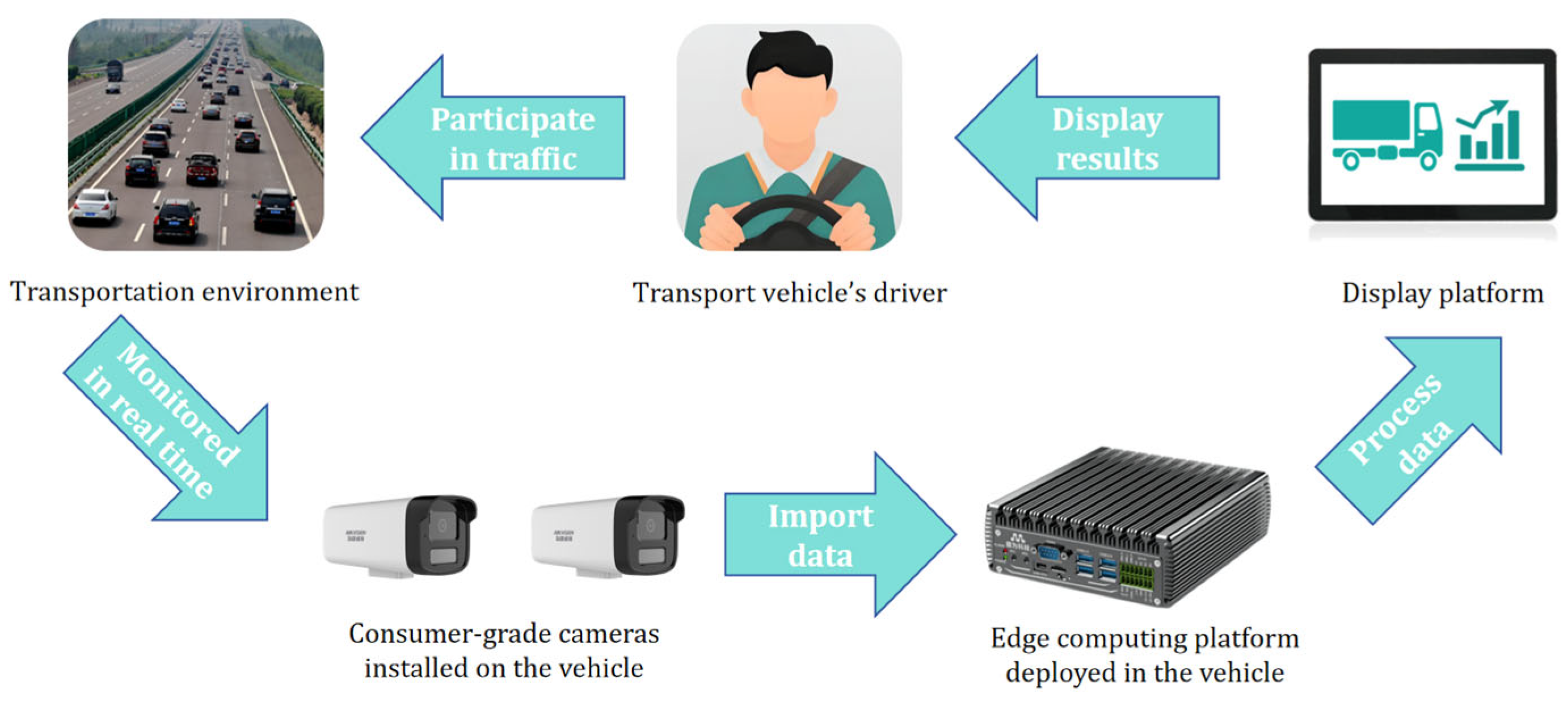The demand for high-end software and hardware facilities results in excessively high costs [23]. To tackle this issue, the YOLOv8 object detection algorithm, along with monocular and binocular camera ranging, is applied to establish an intelligent monitoring system for the driving environment of explosives transport vehicles. The system uses IP cameras that are flexibly arranged around the vehicle body to capture road images in real time and quickly transmits these images to an edge computing device for fast processing. The processed data will be displayed to the driver in an intuitive visual format, enabling the driver to grasp the dynamics of the surrounding environment of the vehicle in real time. With the help of this intelligent monitoring system, drivers can participate in traffic operation more accurately, so as to effectively monitor and prevent possible accidents. The application process of the system is shown in Figure 1.

The main contributions of this article are as follows:

(1)

A low-cost monitoring solution based on consumer-grade IP cameras and edge computing is proposed, addressing the applicability gap of traditional high-cost systems in older explosives transport vehicles.

(2)

A novel integration of YOLOv8 with hybrid ranging techniques is introduced. The system optimizes binocular ranging by performing stereo matching only within YOLOv8-detected bounding boxes, reducing processing latency by 23.5% and enabling real-time performance on low-cost devices. Additionally, the combination of monocular (fast) and binocular (accurate) ranging ensures rapid warnings for distant obstacles and precise measurements in high-risk proximity zones, tailored to the unique demands of explosive transport environments.

(3)

This study delivers an efficient, reliable, and application-specific monitoring system that meets the stringent safety and efficiency requirements of explosives transport vehicles. The system’s performance is rigorously validated under real-world conditions, demonstrating its ability to enhance driving safety while maintaining cost-effectiveness.

2. System Architecture and Hardware Layout

2.1. Selection and Layout of Consumer Cameras

Explosives transport vehicles belong to a type of dangerous goods transport vehicles. According to Road Transport Safety Management Measures for Dangerous Goods of China, the speed regulations for dangerous goods transport vehicles are as follows: dangerous goods transport vehicles cannot exceed 80 km per hour on highways and cannot exceed 60 km per hour on other roads. If the speed indicated on road speed limit signs or markings is lower than the prescribed speed, the vehicle shall not exceed the indicated speed limit. Additionally, Article 80 of the Implementation Regulations of the Road Traffic Safety Law of the People’s Republic of China stipulates that when a motor vehicle is driving on a highway and its speed exceeds 100 km per hour, vehicles must maintain a distance of more than 100 m from the vehicle in front of the same lane. When the speed is less than 100 km per hour, and the distance from the vehicle in front of the same lane can be appropriately shortened, the minimum distance should not be less than 50 m. Therefore, while meeting the driving standards of explosives transport vehicles, taking into account the safety requirements of explosives transport vehicles in actual explosives transport and the error of consumer-grade camera ranging, the monitoring standards are set at a speed of 60 km per hour, a safe following distance of 50 m for front and rear vehicles, and a 2 m distance from surrounding vehicles.

Focal length is the distance from the optical center of the lens to the imaging plane. The smaller the focal length of the camera, the stronger its ability to concentrate light, the wider the viewing range, and the closer the viewing distance. Conversely, the larger the focal length of the camera, the weaker its ability to concentrate light, the narrower the viewing range, and the farther the viewing distance. The system monitors two types of distances: the distance between the front and rear vehicles during transportation and the surrounding vehicles. Therefore, based on the optical characteristics of the camera and the functional requirements of the system, the appropriate camera (Tianjin, China) and its parameters are selected, as shown in

Table 2. Camera model selection [24].

	Function	Camera Model	Focal Length	Horizontal Field of View Angle	Detection Distance
I	Monocular camera	DS-2CD1245(D)-LA	12 mm	27°	80 m
II	Binocular camera		4 mm	70°	50 m

.

The schematic diagram of the monitoring range of the binocular camera is shown in Figure 2, where the sector depicts the field of view of a single camera, and the gray part represents the overlap of the two sectors (i.e., the monitoring range of the binocular camera). θ is the horizontal field of view angle of the camera, d is the baseline distance between two cameras, and x is the length of the monitoring blind zone. The length of the monitoring blind zone x is proportional to the baseline distance d, and d can be determined as Equation (1).

$$d=2x\sqrt{{\displaystyle \frac{1-\mathit{cos}\theta }{1+\mathit{cos}\theta }}}$$

(1)

The blind zone distance x of binocular monitoring must be less than the safety threshold of the system. Based on Equation (1) and the monitoring standard of a 2 m surrounding safety distance, the maximum baseline distance d_max of binocular cameras II listed in Table 1 is calculated using Equation (2):

$$\theta =70°,x=2\mathrm{m},d_{max}=2\mathrm{x}\sqrt{{\displaystyle \frac{1-\mathit{cos}\theta }{1+\mathit{cos}\theta }}}=2\times 2\times \sqrt{{\displaystyle \frac{1-0.34}{1+0.34}}}\approx 2.81\mathrm{m}$$

(2)

A box truck (6 m long, 2.2 m wide, and 2.3 m high) was selected to evaluate the camera layout. It is appropriate to specify a monitoring blind zone of 1.5 m for monitoring, so the baseline is 2 m. The resulting camera layout and detection scale, based on the above analysis, are detailed in

Table 3. Camera layout.

	Baseline	Location
I		A, B
II	2 m	a1, a2, b1, b2, c1, c2, d1, d2

and Figure 3.

2.2. Hardware Architecture of the System

The hardware architecture of the system is divided into three core components, as shown in Figure 4:

(1)

Management side: The YOLO target detection model, which is specially designed to identify and locate objects in the image, is trained on the PC. After the training is completed, the model will be deployed to the edge computing device.

(2)

Data acquisition: IP cameras installed in the transport vehicle body are responsible for capturing the environmental image of the vehicle in real time. Through real-time transport protocol (RTSP) and power over Ethernet (PoE), these image data are efficiently transmitted to network switches and then routed to edge computing devices.

(3)

Data processing and display: Edge computing devices quickly and accurately calculate and process the transmitted data. The processed information is converted into an intuitive visual format and displayed on a dedicated monitoring platform for real-time viewing and analysis by drivers or managers.

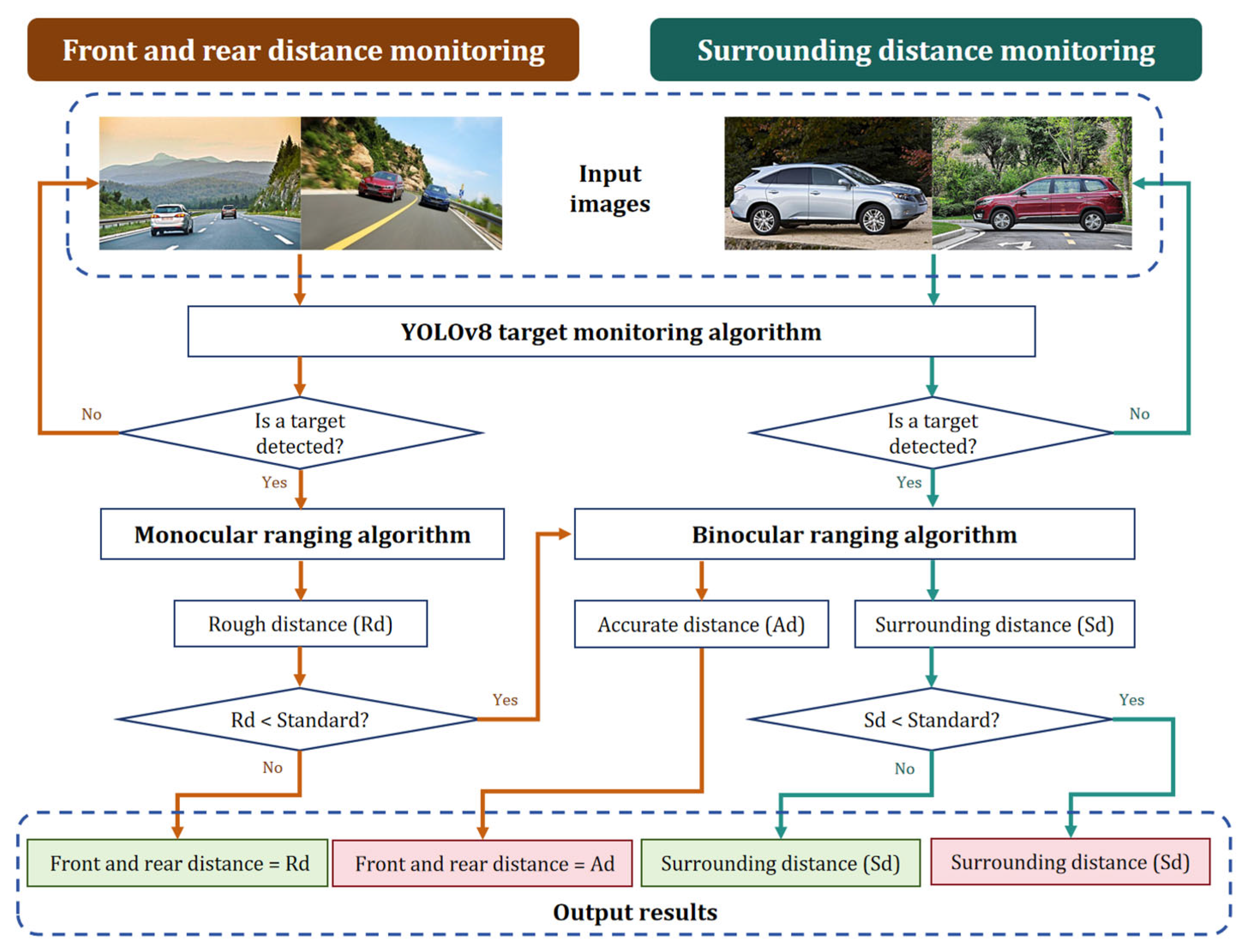
3. System Function Realization

The driving environment intelligent monitoring system has two core functions, and the architecture of function realization is shown in Figure 5.

(1)

Front and rear distance monitoring:

The monocular ranging algorithm provides a faster ranging capability because it processes a single image stream, which reduces the computational complexity compared to the binocular ranging algorithm that requires the analysis of two image streams. Nevertheless, binocular ranging offers higher precision than monocular ranging. The system captures image data in real time through the IP camera and uses the RTSP to transmit the image to the edge computing device. With the help of the YOLOv8 target monitoring algorithm, the system can effectively identify the vehicles in the image. Once the vehicle is detected, the system will input the pixel coordinates of the target to the monocular ranging algorithm to initially determine the vehicle distance. The algorithm uses the monocular camera installed before and after the vehicle body for rough measurement. If the measurement shows that the vehicle distance is less than the preset safety threshold (50 m), the system will start the binocular ranging algorithm and carry out a more precise vehicle distance measurement through the binocular camera before and after the vehicle body and issue an early warning.

(2)

Surrounding distance monitoring:

This function focuses on monitoring vehicles on the side of the vehicle and uses binocular ranging technology for measurement. When the system recognizes the surrounding target, the pixel coordinates of the target are immediately input into the binocular ranging algorithm. Using binocular cameras on both sides of the car body, the system can accurately measure the surrounding distance. Once the measurement result is lower than the set safe distance (2 m), the system will issue an early warning.

3.1. YOLOV8 Target Detection

The comparison of different target detection algorithms is shown in

Table 4. Comparison of target detection algorithms.

Characteristic	YOLOv8	YOLOv5	Faster R-CNN	DETR	SSD
FPS	40 FPS	33.3 FPS	5–10 FPS	<1 FPS	22.22 FPS
mAP@0.5	71.5%	50.5%	75–80%	94%	74%
Robustness	Excellent performance in complex scenes and small targets	Limitation in small target detection	Excellent performance in small targets but slow	High requirements for hardware	Excellent performance in complex scenes but general adaptability to small targets

. Compared with other algorithms, YOLOv8 has significant advantages in terms of accuracy, real-time performance, and robustness [13,14,25].

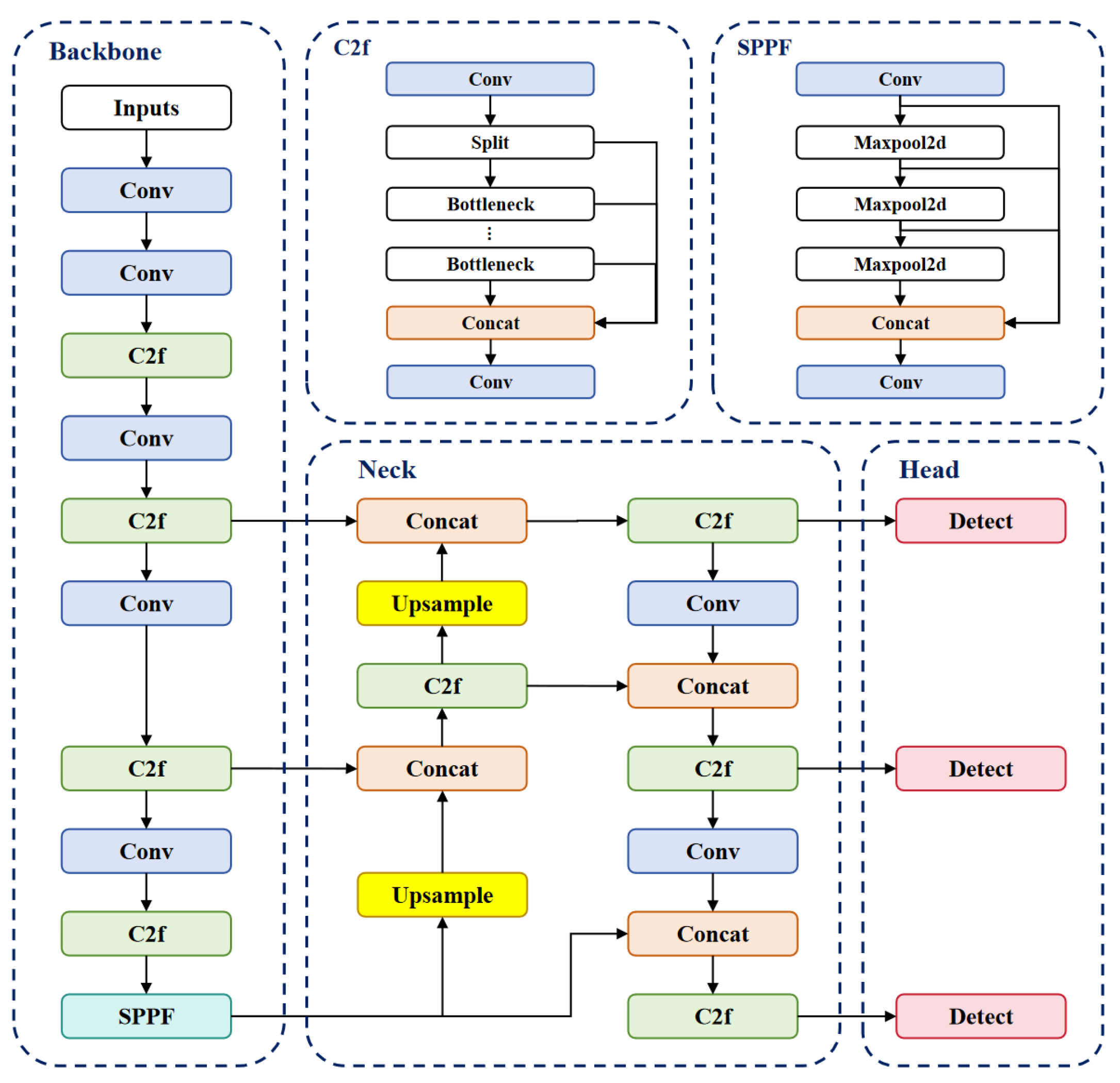
YOLOv8, an object detection model known for its accuracy and fast inference, consists of three key components: Backbone, Neck, and Head. The Backbone extracts features using convolutional and deconvolutional layers, with residual connections and bottleneck structures to optimize network size and performance. It uses the C2f module, which has fewer parameters and better feature extraction than YOLOv5’s C3 module [26]. The Neck module enhances image representation by merging features from different stages of the Backbone, including an SPPF module, a PAA module, and two PAN modules. The Head module handles object identification and classification, with a detection head made up of convolutional and deconvolutional layers using global average pooling to produce the classification results. The network’s structure is illustrated in Figure 6.

Dataset acquisition is crucial for object detection. The intelligent detection system mainly identifies vehicles using a dataset obtained from the open-source UA-DETRAC. To enhance training accuracy, data augmentation techniques are essential. Initially, the training data undergo custom augmentation. Subsequently, the input data are enhanced with color jitter, random horizontal flipping, and random scaling by 10%.

The image, regarded as a collection of pixels, can be expressed as a matrix. YOLOv8 analyzes the input image, capturing its features through feature extraction technology. After calculations, the program identifies objects and provides their locations and labels. This process is realized by the trained weights, which are the core of the algorithm. These weights form the basis for image reasoning and target identification, equivalent to the criteria and standards used in the recognition process. 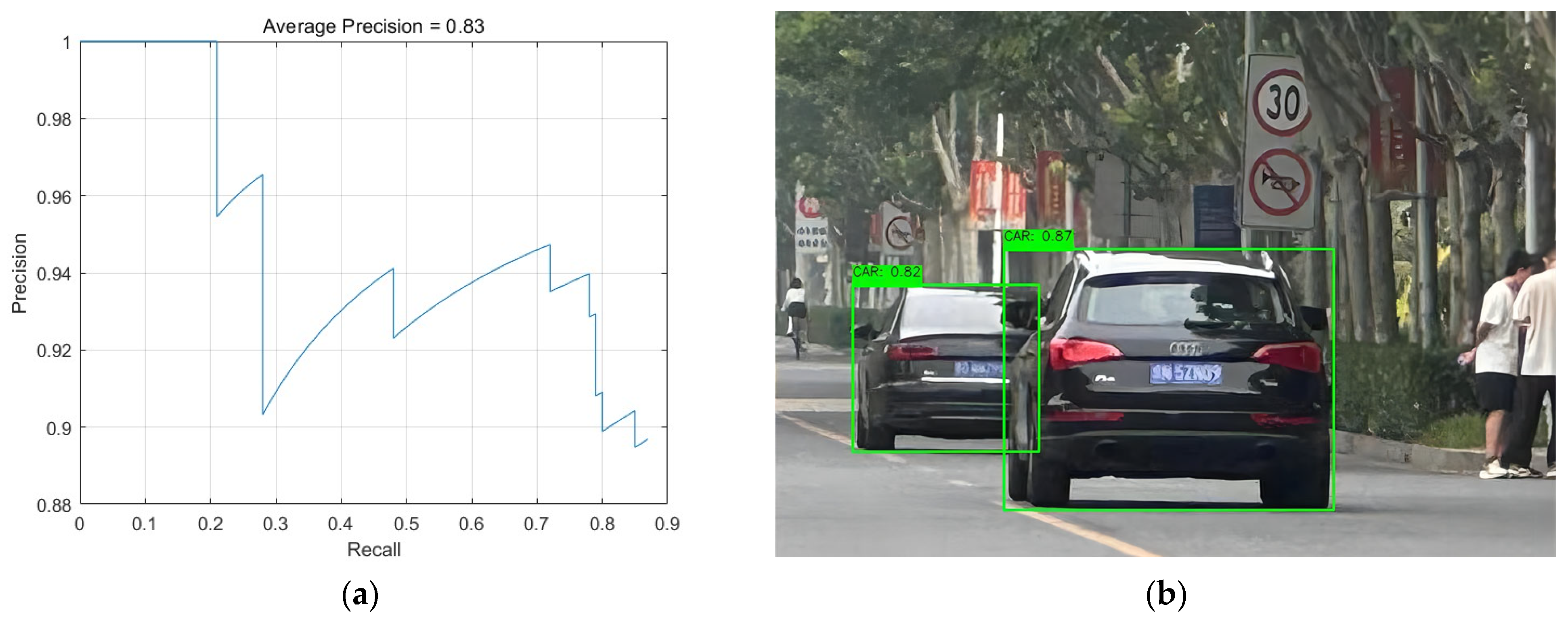Figure 7a illustrates the model’s performance in target monitoring in terms of accuracy and recall at various thresholds.

Assuming that there are only two types of targets to be classified, positive and negative, the following four metrics are used: (1) TP (true positive): the number of positive examples that are correctly identified as positive; (2) FP (false positive): the number of negative examples that are incorrectly identified as positive; (3) TN (true negative): the number of negative examples that are correctly identified as negative; (4) FN (false negative): the number of positive examples that are incorrectly identified as negative.

Precision measures the accuracy of model predictions, indicating the proportion of true positives within the predicted positives.

$$Precision={\displaystyle \frac{TP}{TP+FP}}$$

(3)

Recall indicates the proportion of actual positives correctly identified by the model, reflecting its comprehensiveness.

$$Recall={\displaystyle \frac{TP}{TP+FN}}$$

(4)

Average precision (AP), the area under the precision–recall curve, measures the model’s overall performance across all thresholds and is a key indicator of its effectiveness. A high AP value indicates that the model maintains high accuracy and recall across different thresholds, enhancing its application effectiveness.

To enhance the model’s cross-platform deployment capability, we convert the YOLOv8-trained weights into the versatile ONNX format. This conversion significantly improves the model’s compatibility and applicability across various platforms. We then deploy the model on the edge device, enabling the YOLOv8 target detection algorithm to operate effectively. The detection performance is depicted in Figure 7b.

3.2. Monocular Camera Rough Distance Measurement

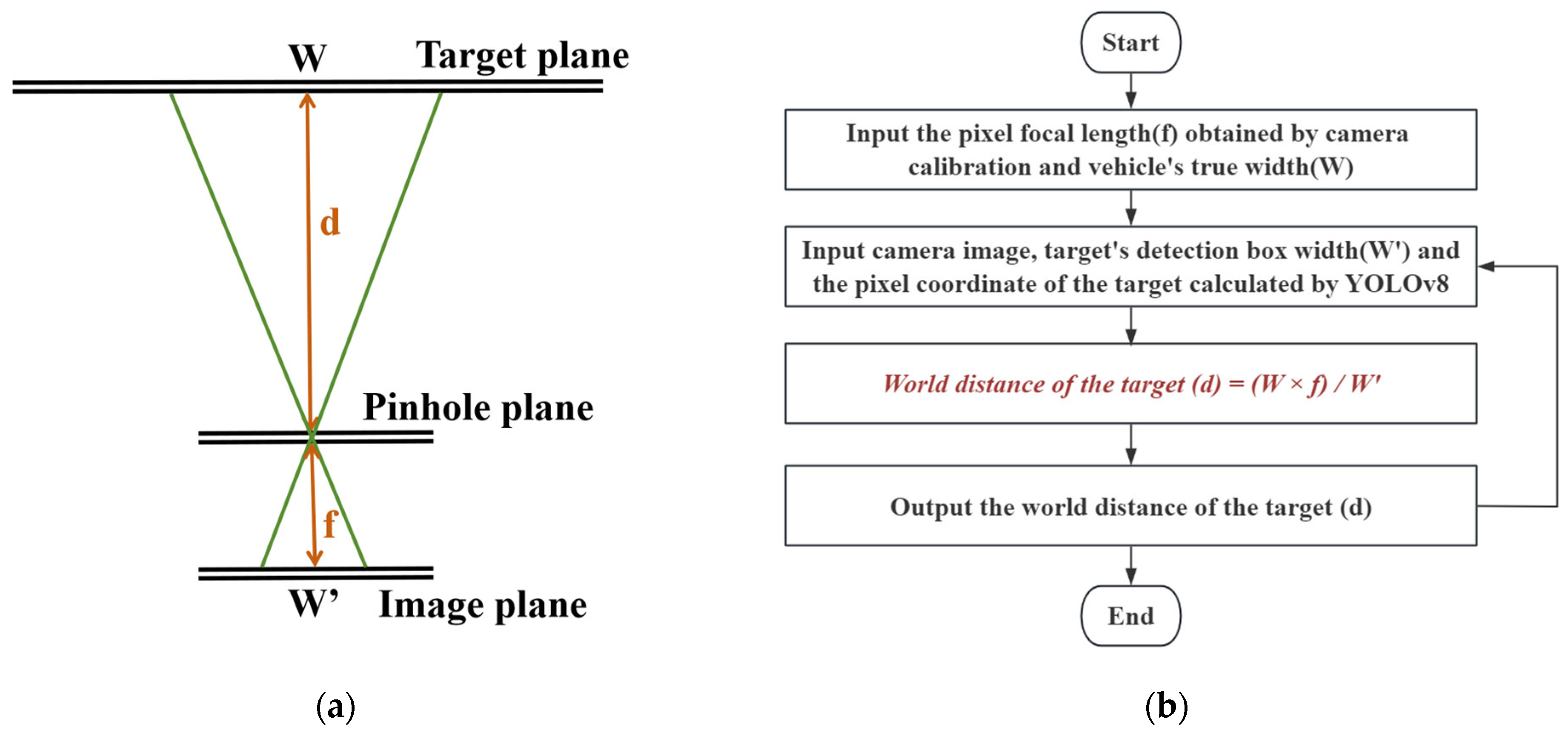
According to the principle of camera imaging, the size of the object in the camera image is proportional to its actual size and related to the focal length. Thus, a similar triangle method can be used for the monocular camera coarse distance measurement. W is the actual width of the object, W′ is the pixel width of the object on the imaging plane, d is the distance between the object and the camera lens, and f is the focal length of the camera. The proportional relationship between the object width and distance is derived from the similarity of triangles. Using this relationship, the distance between the object and the camera lens can be calculated as shown in Equation (5).

$$d={\displaystyle \frac{W\times f}{W^{\prime }}}$$

(5)

Firstly, the camera is calibrated to determine its pixel focal length. Subsequently, this focal length and the true width of the vehicle (W) are input into the system. The image is then imported, and the system is provided with the target detection box width (W′) calculated by YOLOv8, as well as the pixel coordinates of the target. Using these values, the target’s real-world distance is calculated using Equation (5). The final ranging result is then output. The schematic diagram and flow chart of the monocular ranging algorithm are shown in Figure 8.

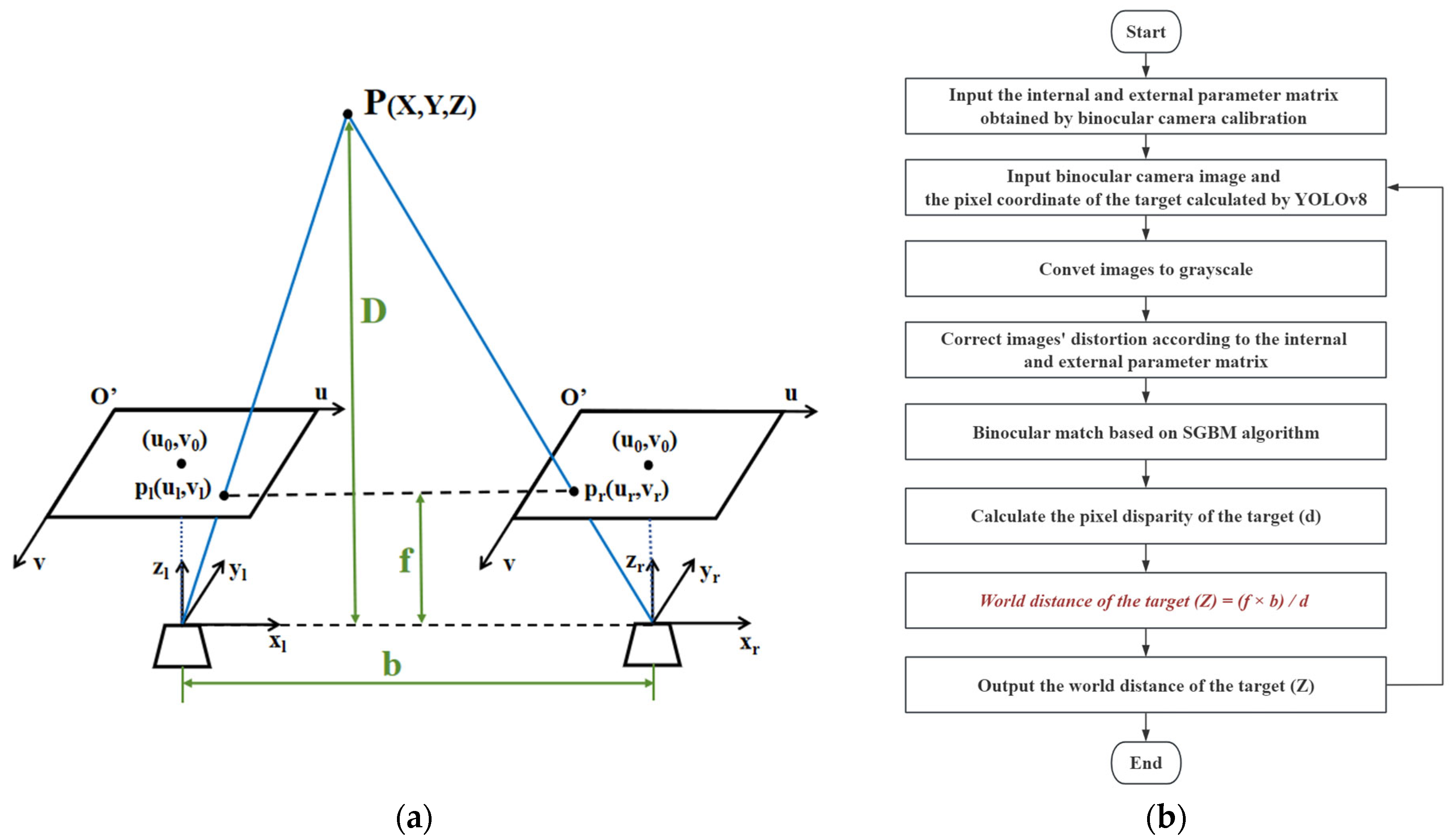
3.3. Binocular Camera Accurate Distance Measurement

A binocular camera consists of two cameras separated by a baseline distance, capturing the object in 2D images. The object’s distance is calculated by measuring the pixel disparities. The Bouguet polar line correction method is used to ensure that the imaging origin coordinates of the left and right camera views are consistent, the optical axes of the two cameras are parallel, the left and right imaging planes are coplanar, and the polar lines are aligned. Using the internal parameters, rotation, and translation matrices from camera calibration, the camera views are adjusted and aligned through rotation and translation.

By observing the object through a binocular lens and calculating the parallax d, combined with parameters such as the baseline distance b and angle of view of two cameras, the three-dimensional coordinates of the object can be calculated using the principle of triangulation, and then the distance D of the object can be calculated using Equation (6). (f is the focal length of the cameras; X, Y, and Z are the global coordinates of the object; and x_l, x_r, y_l, and y_r are the projection coordinates of the object in the left and right cameras.) The schematic diagram of the binocular ranging principle is shown in Figure 9a.

$${\displaystyle \frac{D}{f}}={\displaystyle \frac{X}{x_l}}={\displaystyle \frac{X-b}{x_r}}={\displaystyle \frac{Y}{y_l}}={\displaystyle \frac{Y}{y_r}},D={\displaystyle \frac{f\times b}{x_l-x_r}}={\displaystyle \frac{f\times b}{d}}$$

(6)

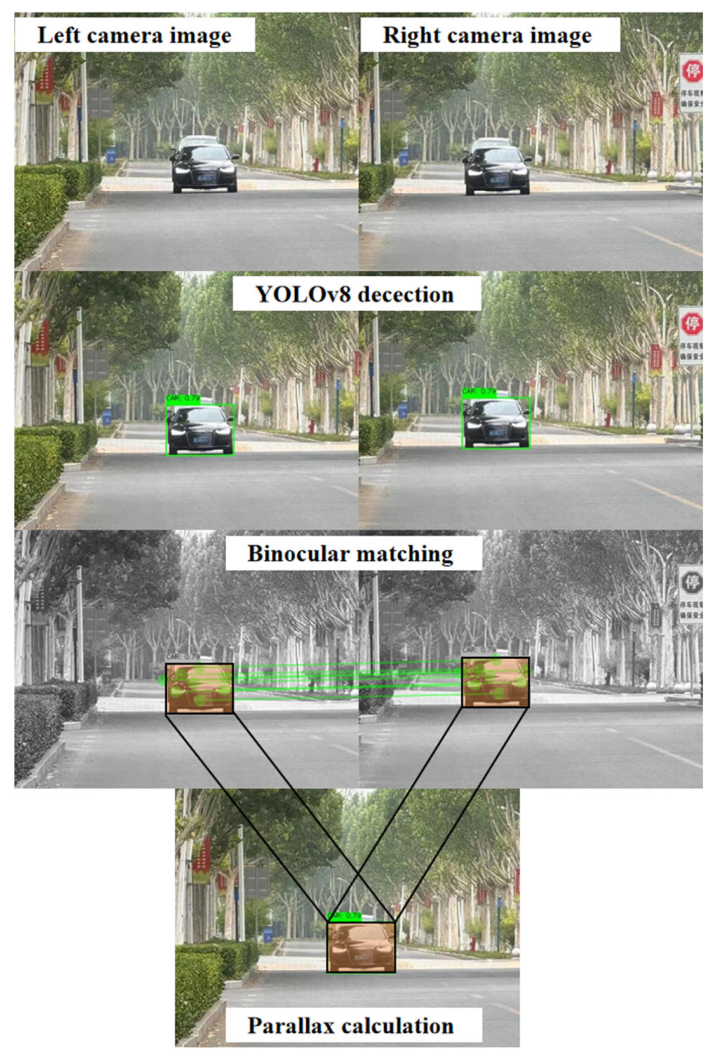
Initially, binocular camera calibration is conducted to derive the internal and external parameter matrices essential for rectifying the binocular camera system. Subsequently, the image captured by the binocular camera and the target’s bounding box pixel coordinates, as ascertained by the YOLOv8 algorithm, are input into the system. The image undergoes conversion to grayscale, and distortion is rectified utilizing the calibrated internal and external parameter matrices. Thereafter, the Semi-Global Block Matching (SGBM) algorithm is engaged to perform stereo matching, which ascertains just the pixel parallax at the target’s bounding boxes. Armed with these data, the target’s real-world distance is computed employing Equation (6). Finally, the calculated world distance of the target is output. The flow chart of the binocular ranging algorithm is shown in Figure 9b and Figure 10.

4. Results and Discussion

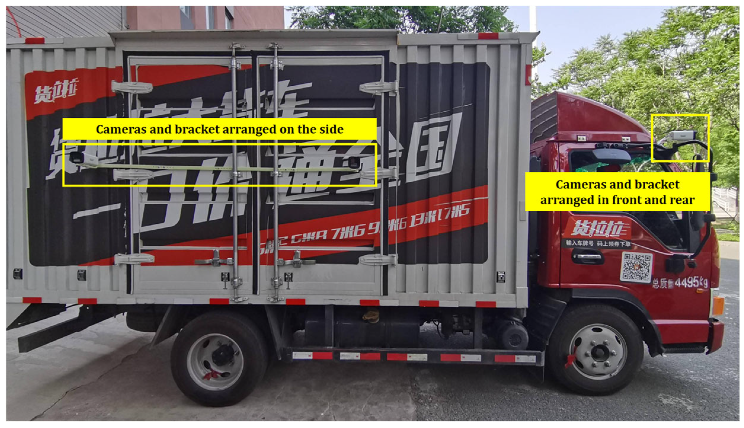
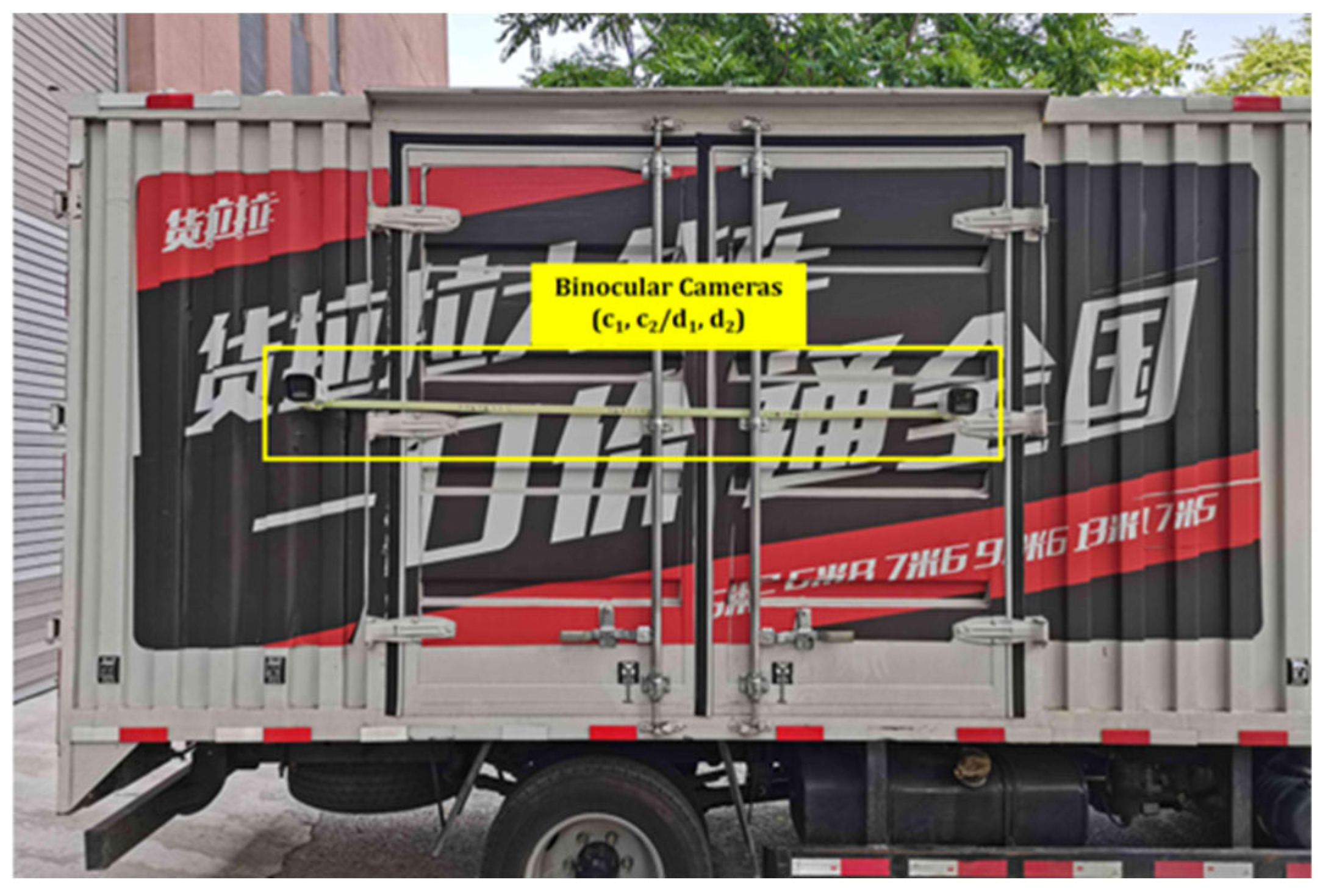
To verify the feasibility and scalability of the hardware and software solutions proposed in this system, as shown in Figure 11, an experiment was conducted on a transport vehicle measuring 6 m in length, 2.2 m in width, and 2.3 m in height. The IP cameras and camera layout utilized in the experiment are detailed in Table 2 and Table 3 of Section 2.1. The cameras, switches, and edge computing device are interconnected via network cables. The switches and edge computing device are powered by vehicle power supply. The configuration of the edge computing device [27] and the algorithmic environment of the system during the test are presented in

Table 5. Hardware and software configuration.

Edge Computing Device: TW-T506S		System’s Algorithmic Environment
Processor	NVIDIA Jetson NX	Package	Version
		colored logs	15.0.1
AI	21TOPS	flat buffers	24.3.25
		humanfriendly	10.0
CPU	6-core NVIDIA Carmel ARM® v8.2 64-bit CPU 6MB L2 + 4MB L3	mpmath	1.3.0
		numpy	1.24.4
GPU	384-core NVIDIA Volta™ GPU with 48 Tensor Cores	onnxruntime	1.17.3
		opencv-python	4.9.0.80
Memory	8 GB 128-bit LPDDR4x 51.2GB/s	packaging	24.0
		pillow	10.3.0
Storage	1× 16 GB eMMC 5.1 1× M.2 Key M NVMe 2280	pip	24.0
		protobuf	5.26.1
DL Accelerator	2× NVDLA Engines	pyreadline3	3.4.1
		setuptools	68.2.2
Video output	1× HDMI 2.0 @ 4Kp60	sympy	1.12
		wheel	0.41.2

.

To ensure the camera’s safety during the experiment and establish a fixed distance between the binocular cameras, an adjustable bracket, specifically designed for the binocular camera and fabricated using 3D printing technology with photosensitive resin material, was created. In this test, we bolted the bracket 2 m above the ground surface to the vehicle’s body. However, in actual transportation scenarios, the bracket’s fixed position should be carefully planned based on the shape and structure of the transport vehicle to further ensure the camera’s safety during the transportation of explosives.

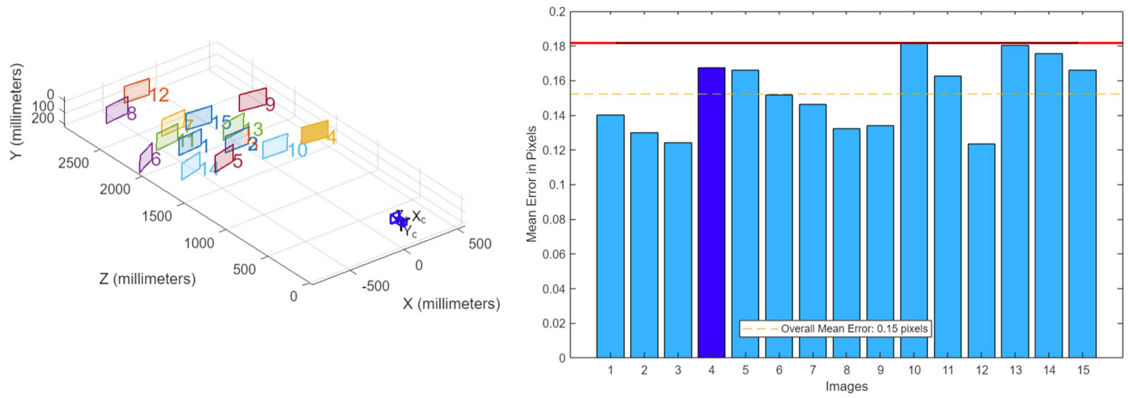
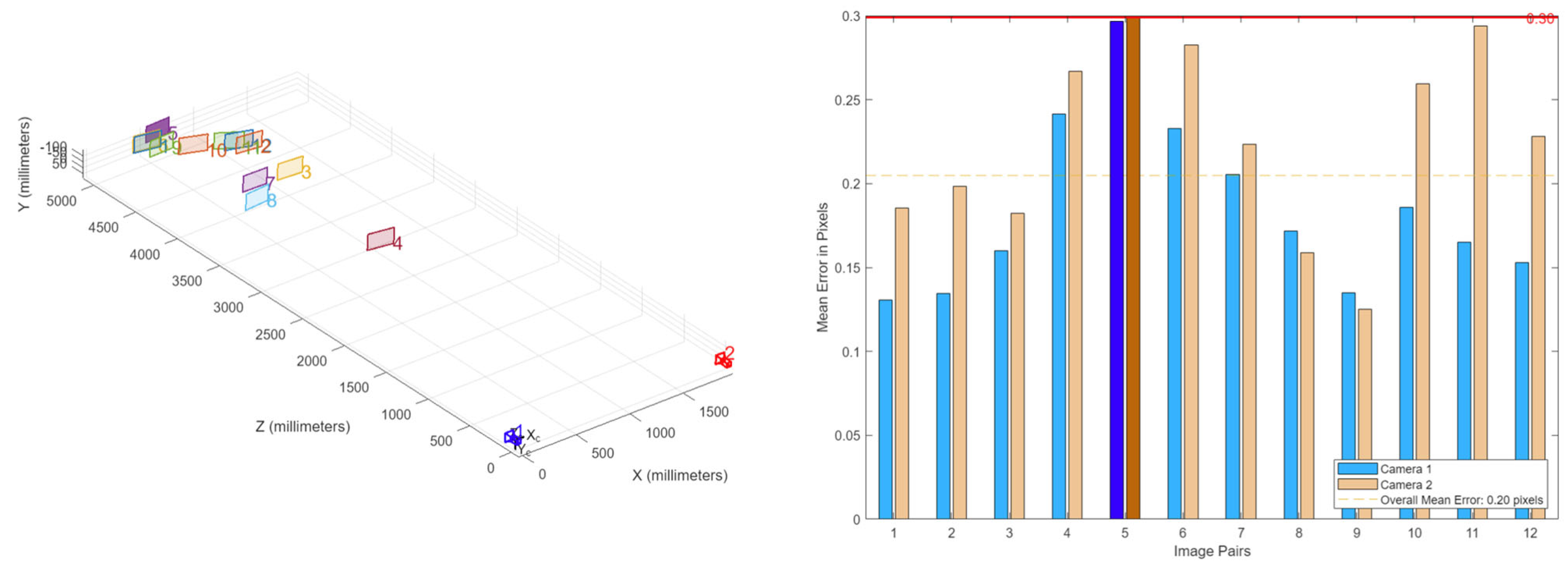
4.1. Monocular and Binocular Camera Calibrations

The checkerboard calibration method is used to calibrate the monocular camera and the binocular camera with a baseline distance of 2 m. The calibration board is a Zhang Zhengyou checkerboard with a grid side length of 28 mm and a black and white grid count of 10 × 7. The reprojection error is obtained by calibration, and the points with a large error are selected for elimination. Finally, the pixel focal length of the monocular camera and the internal and external parameter matrices of the binocular camera are calculated. As shown in Figure 12 and Figure 13, the reprojection errors of the monocular and binocular camera calibration meet the requirements.

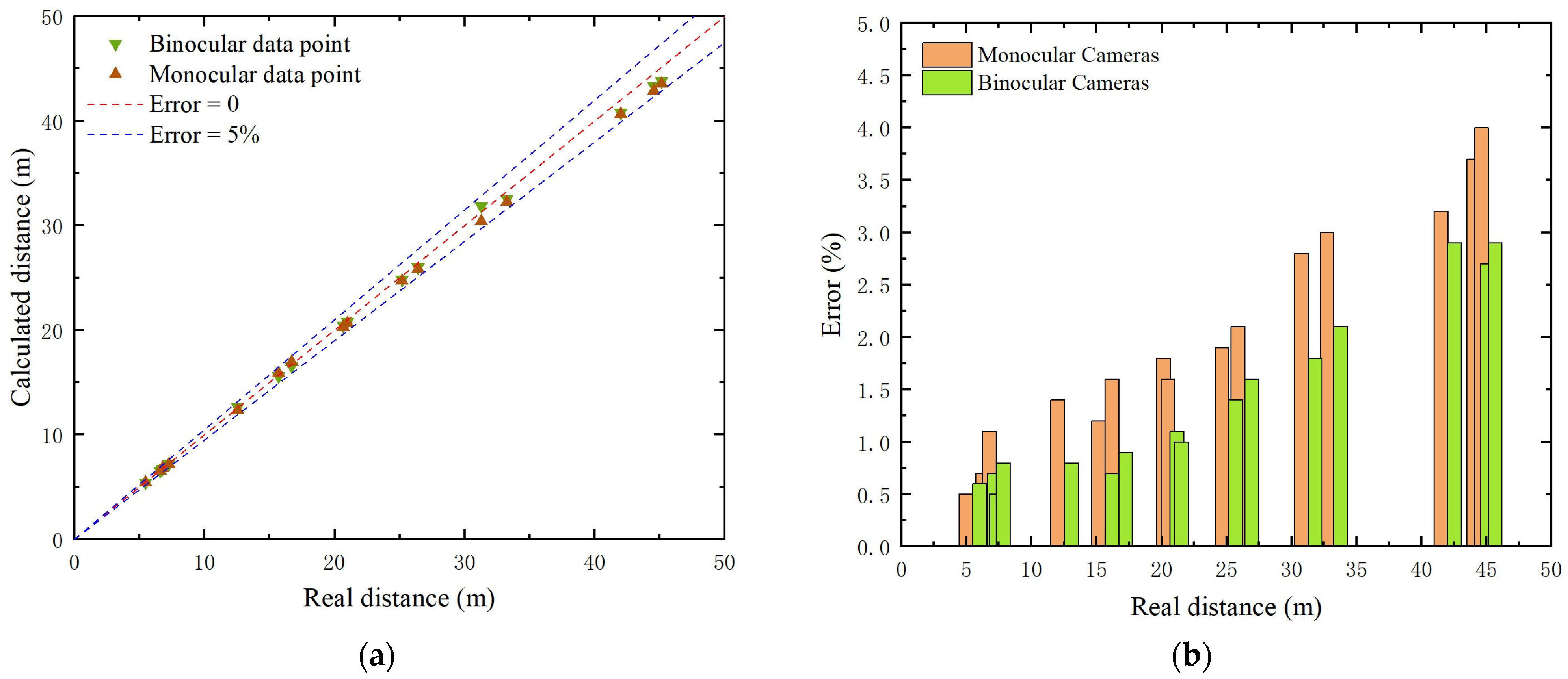
4.2. Front and Rear Distance Monitoring Test

With reference to the 50 m safe distance standard specified in Section 2.1, in the range of 50 m, we used the monocular cameras (A, B) and the binocular camera (a₁, a₂, b₁, b₂) to perform monocular and binocular ranging tests on 20 groups of different distances. The calculated distances (Cd) are recorded, and the maximum running time of the algorithm in the experiment is 0.13 s (the minimum FPS for image reasoning and calculation in the experiment is 7.7 f/s). The distance in the experiment is calculated by monocular and binocular ranging algorithms, while the real distance (Rd) is measured by the laser range finder. The test arrangement is shown in Figure 14. The error (E) calculation is based on Equation (7), and the results are shown in Figure 15.

$$E={\displaystyle \frac{|Cd-Rd|}{Rd}}\times 100\%$$

(7)

As shown in Figure 15, the measurement error of the front and rear distance of the system is controlled within 5% in the range of 50 m, which meets the requirements of error in actual driving. Compared with monocular ranging, binocular ranging shows higher accuracy. In addition, the accuracy of monocular and binocular ranging is proportional to the target distance.

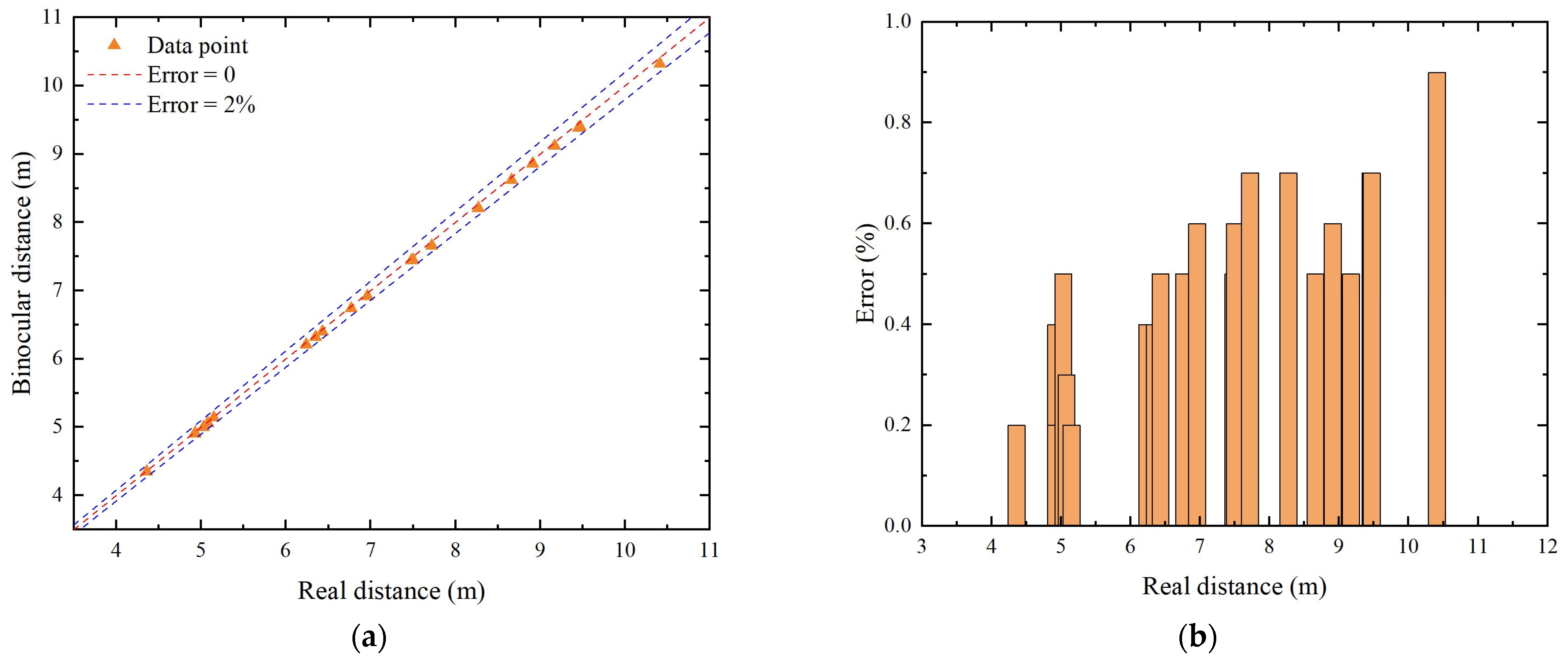
4.3. Surrounding Distance Monitoring Test

With reference to the 2 m safe surrounding distance standard specified in Section 2.1, in the range of 15 m, we used the binocular cameras (c1, c2, d1, d2) to perform binocular ranging tests on 20 groups of different distances. The same as in Section 4.2, the distance in the experiment is calculated by binocular ranging algorithms, while the real distance (Rd) is measured by the laser range finder. The test arrangement is shown in Figure 16. The results are shown in Figure 17.

As shown in Figure 17, the measurement error of the surrounding distance of the system is controlled within 2% in the range of 5 m, which meets the requirements of error in actual driving. And the accuracy of the binocular ranging is proportional to the target distance too.

4.4. FPS Comparative Analysis Test

The FPS (Frames Per Second) of an algorithm refers to the number of image frames that the algorithm can process within a unit of time. It is an important metric for measuring the real-time performance and efficiency of an algorithm. The higher the FPS, the better the real-time performance of the algorithm. The FPS can be calculated using Equation (8):

$$FPS={\displaystyle \frac{1}{Per-frameProcessingTime}}$$

(8)

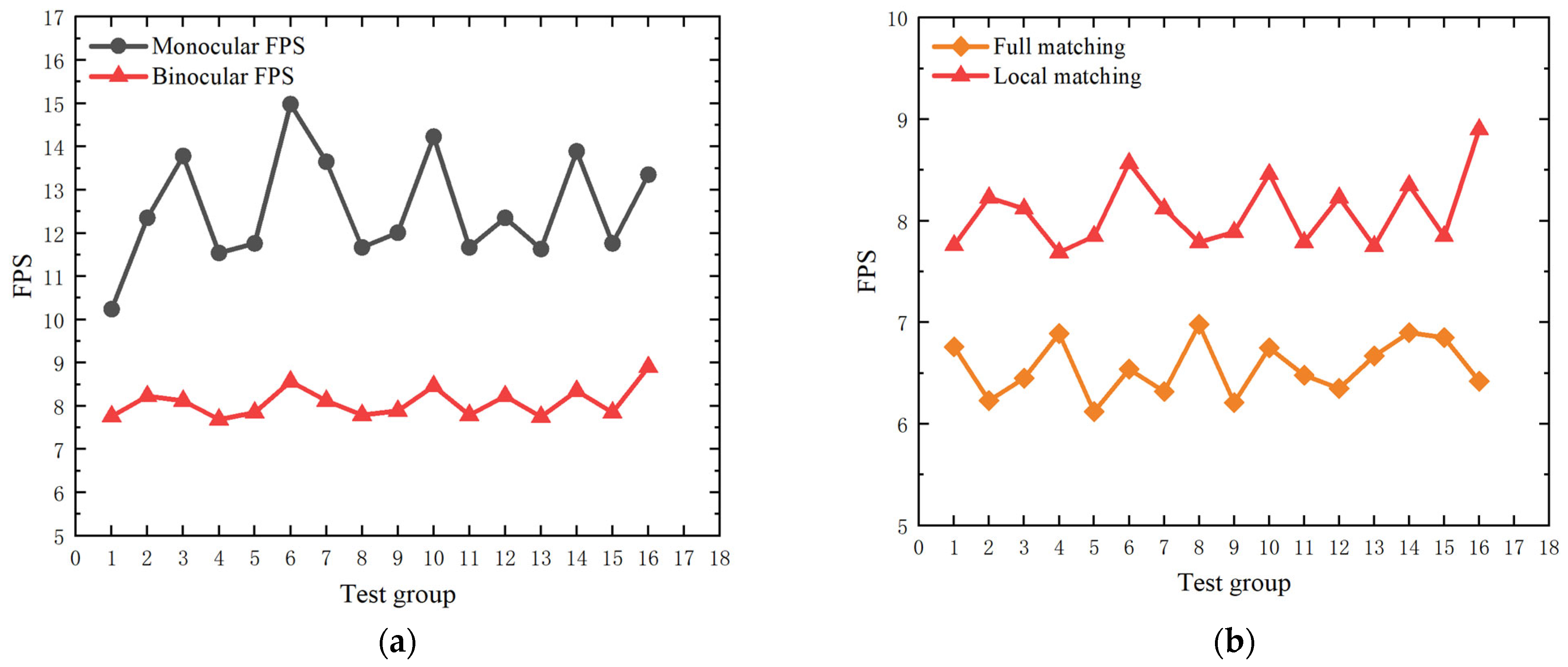
In order to verify the real-time performance of the system, we compared the monocular ranging method and binocular ranging method based on local matching used in the system with the binocular ranging method based on full image matching without optimization and conducted FPS tests on 16 groups of test data. The results are shown in Figure 18.

As shown in Figure 18, compared with the binocular ranging method based on local matching, the FPS of the monocular ranging method is improved by 55% on average; compared with the non-optimized binocular ranging method based on full matching, the FPS of the binocular ranging method based on local matching used in this system is improved by 23.5% on average. Therefore, the system has significant advantages in the real-time performance of early warning and ranging.

4.5. System Visual Display

In order to verify the feasibility of the system in practical application, we designed a front-end visual interface for the system. The design of the interface is shown in Figure 19. The interface displays the actual distance between the front and back of the vehicle and the distance between the surrounding objects in real time in a visual form on the corresponding position around the vehicle. If the detected distance falls below the preset safety threshold, the interface will display the value with a striking red warning sign to immediately attract the driver’s attention. Additionally, the driver can observe the vehicle’s surroundings in real time on the right side of the interface, enabling timely corresponding driving actions and effectively preventing potential risks. In order to ensure driving safety, an audible and visual alarm system will be developed in the future: early warning can be achieved through the linkage of in-vehicle lights and sounds, and when danger is detected, lights and voice prompts will be triggered synchronously so as to improve the driver’s response speed and reduce the risk of accidents [28].

5. Conclusions

This article proposes an intelligent monitoring system for the driving environment of explosives transport vehicles based on consumer-grade cameras. The system uses a consumer-grade IP camera to capture images of road conditions in real time and quickly transmits these images to edge computing devices. On the edge device, combined with deep learning and computer vision technology, target detection and ranging calculation are performed. Subsequently, the processed data are presented to the driver in a visual form so that the driver can grasp the traffic conditions and participate in the traffic operation. The system significantly improves driving safety and helps to effectively prevent traffic accidents.

(1)

A low-cost monitoring solution based on IP cameras and edge computing is proposed, filling the applicability gap of traditional high-cost systems in old transport vehicles. The system captures real-time data via IP cameras and processes them on edge devices, enabling efficient monitoring of the driving environment at a fraction of the cost of traditional systems.

(2)

The system integrates YOLOv8 for target detection with a hybrid ranging approach, combining the speed of monocular ranging and the precision of binocular ranging. This dual-mode strategy ensures rapid warnings for distant obstacles and accurate measurements in high-risk proximity zones, tailored to the unique demands of explosive transport.

(3)

A key innovation is the optimized binocular ranging algorithm, which performs stereo matching only within YOLOv8-detected bounding boxes. This optimization reduces processing latency by 23.5%, enabling real-time performance on low-cost edge devices while maintaining high accuracy.

(4)

Tests show that the system works well in real-world conditions. It keeps distance measurement errors below 5% within a 50 m range, meeting the safety needs of explosive transport. This proves that the system is reliable and robust for actual driving scenarios.

Research shortcomings and prospects: This study found that the current system, relying on consumer-grade cameras, is limited in performance under extreme lighting conditions. Additionally, its practical effectiveness in complex traffic scenarios such as rain, snow, and nighttime has not been fully validated. In future research, we will explore more advanced camera technologies to enhance system performance under extreme lighting conditions and further validate its application in complex traffic scenarios, aiming to provide more reliable outcomes for relevant research and practice.