Article

Research on Structural Mechanics Stress and Strain Prediction Models Combining Multi-Sensor Image Fusion and Deep Learning

School of Computer Science, Cornell University, Ithaca, NY 14853, USA
*
Author to whom correspondence should be addressed.
Appl. Sci. 2025, 15(7), 4067; https://doi.org/10.3390/app15074067
Submission received: 2 March 2025 / Revised: 16 March 2025 / Accepted: 27 March 2025 / Published: 7 April 2025

Abstract

:
The integration of multi-sensor imaging and deep learning techniques has emerged as a pivotal innovation in advancing structural mechanics, particularly in the prediction of stress and strain distributions. This study falls within the thematic scope of multi-sensor imaging and fusion methods, emphasizing their crucial role in assessing material behavior under complex conditions. Traditional methodologies, such as finite element methods and classical constitutive models, often fall short in capturing the intricacies of heterogeneous materials and nonlinear stress–strain relationships. These limitations necessitate a more robust computational framework capable of addressing material variability and computational efficiency challenges. To this end, we propose the Stress–Strain Adaptive Predictive Model (SSAPM), which synergizes mechanistic modeling with data-driven corrections. Leveraging hybrid representations, adaptive optimization strategies, and modular architectures, SSAPM ensures precision by embedding physics-informed constraints and reduced-order modeling for computational scalability. Experimental validations underscore the model’s capability to generalize across diverse structural scenarios, outperforming conventional approaches in accuracy and efficiency. This work establishes a transformative pathway for incorporating multi-sensor data fusion into structural analysis, advancing the predictive power and applicability of stress–strain models.

1. Introduction

Structural mechanics plays a critical role in ensuring the safety and reliability of engineering systems [1], as accurate predictions of stress and strain are essential for assessing material performance and structural stability [2]. Traditional methods, such as finite element analysis (FEA) and symbolic AI, rely on predefined rules and physics-based models but struggle with scalability and real-world complexity [3]. The high computational cost of these simulations further limits their application in large-scale or real-time scenarios [4]. To address these limitations, data-driven approaches emerged, utilizing statistical modeling and classical machine learning (ML) techniques like regression and support vector machines [5]. While these methods improved adaptability by training on empirical data [6], they lacked the ability to capture deep hierarchical features and multi-sensor interactions, limiting their effectiveness in modeling complex stress–strain behaviors [7]. The sensitivity of traditional ML models to data quality and variability remained a significant challenge.
The advent of deep learning revolutionized structural mechanics by providing models capable of learning intricate stress–strain relationships from data [8]. Convolutional neural networks (CNNs) and transformer-based architectures significantly enhanced predictive accuracy by extracting rich features from multi-sensor inputs [9]. Hybrid approaches, such as physics-informed neural networks (PINNs) and FEA-integrated deep learning models [10], have further improved generalizability by embedding physical laws directly into learning frameworks [11]. These methods are particularly beneficial for scenarios with scarce labeled data, as they reduce the reliance on large-scale experimental datasets [12]. Despite these advancements, challenges such as high computational demands [13], interpretability issues [14], and the need for domain-specific adaptations persist, limiting their direct applicability to structural mechanics [15]. The integration of deep learning with uncertainty quantification techniques further enhances trust in predictive models [16], enabling more reliable decision-making in engineering applications [17].
Multi-sensor image fusion offers a powerful solution by integrating diverse imaging modalities, including infrared thermography, digital image correlation (DIC), and X-ray computed tomography [18]. By combining pixel, feature, and decision-level fusion techniques, these methods enable the extraction of multi-scale and multi-physics features crucial for understanding complex mechanical behaviors [19]. Applications in crack detection, residual stress analysis, and fatigue life assessment demonstrate the effectiveness of fused data in enhancing diagnostic precision [20]. Advanced fusion algorithms, such as principal component analysis (PCA) and deep learning-based fusion networks, mitigate noise and artifacts while improving spatial resolution [21]. Emerging research also explores real-time fusion strategies that adapt dynamically to changing environmental or loading conditions, further advancing structural health monitoring capabilities [22]. The synergistic use of fused data not only enhances the accuracy of stress–strain predictions but also facilitates adaptive diagnostics in varying operational conditions [23].
The integration of multi-sensor image fusion with deep learning presents a transformative approach for stress and strain prediction [24]. This synergy allows deep learning models to leverage enriched datasets, extracting intricate patterns and improving prediction accuracy [25]. Techniques such as 3D convolutional neural networks and attention-based architectures capture spatial, temporal, and cross-modal dependencies, enhancing the robustness of structural assessments [26]. Transfer learning and self-supervised learning approaches reduce computational costs and data requirements by pre-training models on generic datasets before fine-tuning them for specific applications [27]. Uncertainty quantification mechanisms enhance trust in automated systems by providing confidence intervals for predictions [28]. As research in this domain continues to evolve [29], key focus areas include real-time implementation [30], scalability, and the integration of emerging sensor technologies to further enhance structural diagnostics and decision-making [31]. Future advancements will likely focus on improving the interpretability of deep learning models in structural mechanics applications [32], optimizing computational efficiency, and incorporating domain-specific constraints into neural architectures [33]. Interdisciplinary collaborations between structural engineers and AI researchers will drive the development of more reliable and adaptable prediction models [34]. The combination of multi-sensor fusion, deep learning, and physics-informed models represents a paradigm shift in structural health monitoring and predictive maintenance strategies [35].
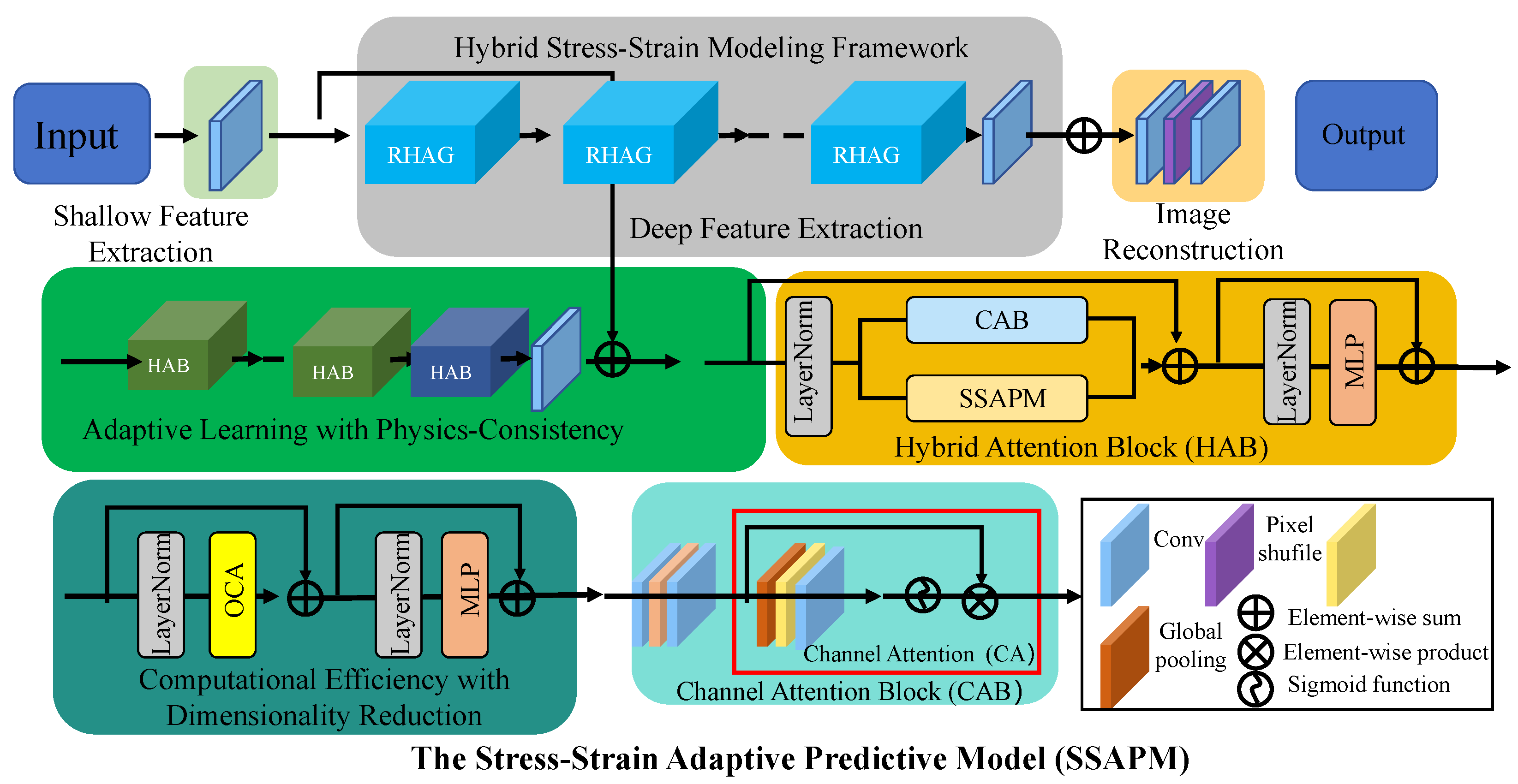
Despite significant progress in stress–strain prediction models, existing approaches still face several key challenges. Traditional finite element methods and classical constitutive models struggle to capture the complex nonlinear stress–strain behaviors of heterogeneous materials, leading to limitations in accuracy. Data-driven machine learning models, while improving predictive performance, often lack physical interpretability and generalizability due to their reliance on empirical training data. Computational efficiency remains a concern, as high-fidelity simulations demand significant processing power, limiting real-time applications in structural analysis. To address these limitations, this study introduces the Stress–Strain Adaptive Predictive Model (SSAPM), which integrates multi-sensor image fusion with a domain-aware deep learning framework. By bridging the gap between physics-based modeling and machine learning, our approach establishes a more robust and scalable framework for stress–strain prediction in structural mechanics.
We summarize our contributions as follows:
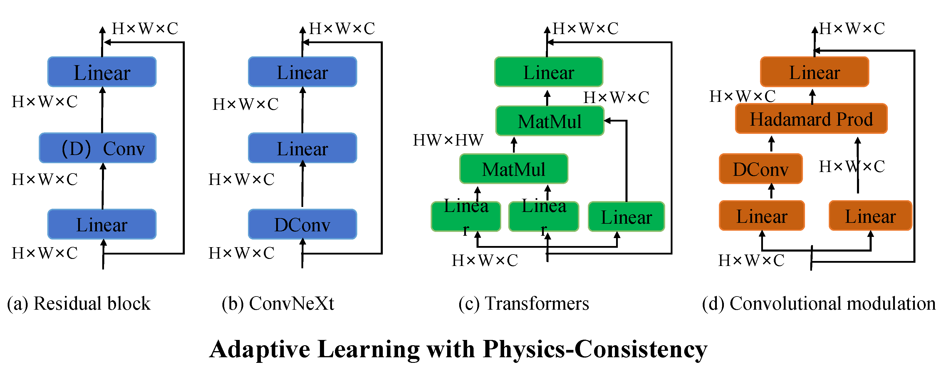
  • A hybrid modeling approach that combines mechanistic stress–strain relationships with data-driven corrections to improve accuracy while maintaining physical interpretability.
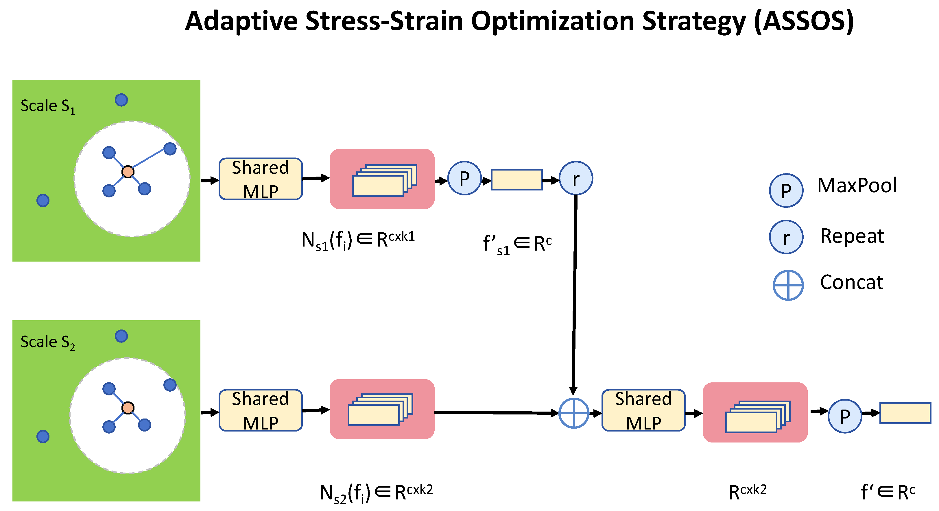
  • A hierarchical multi-sensor fusion module that effectively integrates thermal, acoustic, and visual imagery for enhanced material behavior prediction.
  • An adaptive optimization strategy that ensures computational efficiency while preserving model precision across diverse structural scenarios.

2. Method

2.1. Overview

Predicting stress and strain in structural mechanics is pivotal for understanding material behaviors under various loads and environmental conditions. This study addresses the prediction problem through an innovative computational framework that integrates theoretical insights with advanced numerical techniques. This subsection outlines the methodological structure of our work. We first define the fundamental problem in structural mechanics by formulating the relationships between stress, strain, and material properties. These are detailed in Section 2.2, where we introduce the governing equations and their mathematical formulations, including boundary conditions and constitutive relations. In Section 2.3, we propose a novel computational model, termed Mechanistic Stress–Strain Predictor (MSSP). This model leverages advanced computational strategies to represent complex material behaviors, particularly in anisotropic or heterogeneous materials. MSSP introduces a modular design that enhances flexibility and scalability in simulating various structural scenarios. In Section 2.4, we present the adaptive optimization techniques embedded within MSSP. These techniques refine predictions through an iterative learning approach that adjusts to discrepancies between modeled outcomes and empirical data. By incorporating domain-specific knowledge and leveraging efficient numerical solvers, the proposed approach effectively minimizes computational overhead while maximizing predictive accuracy.

2.2. Preliminaries

This section formalizes the structural mechanics problem, focusing on stress and strain prediction within materials under external loads. We begin with the foundational principles of continuum mechanics and gradually introduce the mathematical models that underpin our methodology. This formulation serves as the groundwork for our proposed model.
The core equations governing structural mechanics are derived from conservation laws. The equilibrium equation ensures that the internal stresses balance the external forces:
nabla · σ + f = 0 ,
where σ is the Cauchy stress tensor, f is the body force per unit volume, and  nabla · σ represents the divergence of the stress tensor.
The strain tensor quantifies deformation in the material and is derived from the displacement field u :
ε = 1 2 nabla u + ( nabla u ) ,
where ε is the strain tensor and nabla u is the gradient of the displacement field.
Stress–strain relationships define how materials respond to external loads. For linear elasticity, Hooke’s law is given by
σ = C : ε ,
where C is the fourth-order elasticity tensor, and : denotes a double contraction.
For nonlinear materials, constitutive models depend on factors like plasticity or viscoelasticity, and the stress–strain relation is more complex:
σ = F ( ε , ε ˙ , p ) ,
where ε ˙ is the strain rate and p represents internal state variables.
Solving the problem requires specifying boundary conditions:
u = u 0 on Γ u ,
σ · n = t 0 on Γ t ,
where Γ u and Γ t are the boundaries with prescribed displacement u 0 and traction t 0 , respectively, and  n is the outward normal.
The weak form is essential for numerical methods:
Ω ( nabla · σ ) · δ u d Ω + Ω f · δ u d Ω = 0 ,
where δ u is the test function in the admissible space, and  Ω is the domain of interest.
Finite element methods (FEM) are used to discretize the equations. The domain is divided into elements, and the displacement u is approximated as
u i N i u i ,
where N i are the shape functions, and  u i are the nodal displacements.
The discretized equations form a system of equations:
K u = F ,
where K is the global stiffness matrix, u is the nodal displacement vector, and  F is the force vector.
The mathematical framework presented in this study is rooted in the fundamental principles of continuum mechanics and elasticity theory, as established in classical works such as Introduction to the Mechanics of a Continuous Medium [36] and Theory of elasticity [37]. The governing equations, including the equilibrium equation, strain-displacement relations, and constitutive models, are derived from conservation laws and thermodynamic principles. The equilibrium equation follows directly from Newton’s second law applied to a differential volume element, ensuring force balance within the material. The strain tensor definition is derived from the kinematic relationship between displacements and deformations in a continuous medium. The constitutive equation represents Hooke’s law for linear elasticity and extends to nonlinear cases via phenomenological or physically based models, as described in Foundations of solid mechanics [38] and Nonlinear solid mechanics: a continuum approach for engineering science [39]. All these equations are fundamental to computational modeling in structural mechanics, providing a rigorous basis for stress–strain prediction.

2.3. The Stress–Strain Adaptive Predictive Model (SSAPM)

In this section, we introduce the Stress–Strain Adaptive Predictive Model (SSAPM), a comprehensive computational framework designed to predict stress and strain distributions with high accuracy (as shown in Figure 1). The SSAPM combines principles of continuum mechanics with machine learning to address nonlinearities and material heterogeneity. Below, we highlight three core innovations that define the SSAPM.

2.3.1. Hybrid Stress–Strain Modeling Framework

The SSAPM introduces a hybrid representation where the stress tensor σ is expressed as a superposition of a mechanistic component M , grounded in classical constitutive laws, and a data-driven correction term D , designed to capture material complexities and heterogeneities beyond traditional models:
σ = M ( ε , p ) + D ( ε , x ) ,
where ε represents the strain tensor, p denotes state-dependent variables (e.g., plastic strain, internal damage metrics), and  x includes auxiliary factors such as temperature, strain rate, or prior loading history. The mechanistic component M encapsulates elastic and inelastic material behavior. For linear elastic responses, it follows Hooke’s law:
M ( ε ) = C : ε ,
where C is the elasticity tensor, a fourth-order tensor that governs stress–strain relationships in isotropic or anisotropic materials. For nonlinear and inelastic responses, M accounts for additional terms:
M ( ε , p ) = F ( ε ) + H ( p ) ,
where F ( ε ) incorporates nonlinear elastic responses, often through polynomial or exponential functions of ε , and  H ( p ) models plastic deformation or viscoelastic effects.
We considered incorporating viscoelastic effects to account for time-dependent stress–strain behavior. However, since our primary formulation follows a static framework, as defined in Equation (1), the inclusion of viscoelasticity would require a more comprehensive reformulation to explicitly address dynamic effects. Given that viscoelasticity inherently involves time-dependent stress evolution, its presence within a purely static context lacks justification.
The data-driven term D , in contrast, employs a neural network to adaptively learn material behavior from experimental data, expressed as
D ( ε , x ) = Ψ ( ε , x ; Θ ) = i = 1 k α i ϕ i ( ε , x ) ,
where ϕ i are basis functions (e.g., nonlinear activation functions in the neural network), α i are learnable coefficients, and  Θ encapsulates the network parameters. The network is trained to minimize the residual stress:
R = σ exp ( M ( ε , p ) + D ( ε , x ) ) 2 ,
where σ exp denotes experimentally observed stress. This hybridization allows SSAPM to balance theoretical rigor with empirical adaptability, enabling precise predictions of stress–strain behavior under diverse loading conditions. Furthermore, the inclusion of physical constraints, such as enforcing equilibrium:
· σ + f = 0 ,
ensures that the model adheres to fundamental physical principles while flexibly addressing complex material responses. By leveraging these components, SSAPM captures both macroscopic behavior and microstructural influences, bridging the gap between classical theories and modern data-driven approaches.

2.3.2. Adaptive Learning with Physics-Consistency

The SSAPM leverages a robust multi-objective loss function to ensure that its predictions are not only data-driven but also grounded in the fundamental laws of physics (as shown in Figure 2). This hybrid objective simultaneously minimizes the error in predicted stresses while enforcing physical consistency through governing equations. The loss function is defined as
L = λ 1 σ pred σ true 2 + λ 2 · σ pred f 2 + λ 3 R ( Θ ) ,
where σ pred and σ true represent the predicted and true stress tensors, respectively, f denotes external forces, and  R ( Θ ) is a regularization term designed to constrain the complexity of the neural network parameters Θ . The terms λ 1 , λ 2 , and  λ 3 are weighting factors that balance the contributions of data fidelity, equilibrium satisfaction, and regularization.
To ensure physical adherence, the second term in the loss function incorporates the equilibrium constraint:
· σ pred + f = 0 ,
where · σ pred represents the divergence of the predicted stress tensor. This enforces that the internal stresses within the material equilibrate with the external forces. Furthermore, the regularization term R ( Θ ) penalizes overly complex solutions, typically defined as
R ( Θ ) = Θ 2 2 + α ε Ψ 2 ,
where Θ 2 2 controls the size of the model parameters, and the gradient regularization ε Ψ 2 smoothens the data-driven component Ψ with respect to strain ε , ensuring physical plausibility.
The optimization process dynamically adjusts Θ , the parameters of the data-driven correction term Ψ , using a gradient-based method such as Adam or L-BFGS. The gradients of L with respect to Θ are computed as
L Θ = 2 λ 1 σ pred σ true σ pred Θ + 2 λ 2 · σ pred f ( · σ pred ) Θ + λ 3 R ( Θ ) Θ .
The equilibrium constraint term can also incorporate boundary conditions, such as stress-free surfaces or prescribed traction, encoded as
σ pred · n = t ,
where n is the outward normal vector on the boundary, and  t is the applied traction. This ensures that the predicted stress distributions are consistent with both internal equilibrium and external boundary conditions. By iteratively minimizing L , the SSAPM achieves a harmonious integration of data-driven adaptability and physical realism. The adaptive learning framework enables the model to generalize across varying material heterogeneities and nonlinear behaviors, while the regularization and physics-consistency terms prevent overfitting, ensuring robustness and interpretability. This holistic optimization process empowers SSAPM to tackle complex material modeling challenges with precision and reliability.

2.3.3. Computational Efficiency with Dimensionality Reduction

Computational efficiency is a critical requirement for large-scale material simulations, especially when dealing with high-dimensional systems and complex geometries. To address this, the SSAPM integrates a projection-based dimensionality reduction technique to simplify strain tensor computations without compromising accuracy. The strain tensor ε is expressed as a projection onto a low-dimensional subspace:
ε i = 1 k α i Φ i ,
where Φ i are orthogonal basis tensors, α i are projection coefficients, and k represents the reduced dimensionality, which is significantly smaller than the full tensor space dimensionality. The basis tensors Φ i are derived using spectral decomposition of a strain covariance matrix obtained from training data, ensuring that the low-dimensional basis captures the most significant strain modes. Mathematically, this is achieved by solving:
C ε Φ i = λ i Φ i ,
where C ε is the covariance matrix of strain tensors, λ i are eigenvalues, and  Φ i are the corresponding eigenvectors.
This reduction not only decreases computational costs but also enhances numerical stability by filtering out noise and irrelevant strain components. The coefficients α i are computed through projection:
α i = V ε : Φ i d V ,
where V represents the material volume under consideration. By retaining only the dominant k modes (corresponding to the largest eigenvalues), the SSAPM effectively compresses the strain data, reducing storage and computational demands.
The reduced strain representation is seamlessly integrated into the hybrid stress model. The mechanistic term M and data-driven correction D are reformulated in terms of the reduced basis:
M ( ε ) = i = 1 k α i M ( Φ i ) , D ( ε , x ) = i = 1 k α i Ψ ( Φ i , x ; Θ ) ,
ensuring that the computational efficiency extends to all stages of the SSAPM pipeline.
The modular design of SSAPM incorporates specialized components to leverage this dimensionality reduction effectively. A feature extractor preprocesses auxiliary data, such as temperature or loading rates, reducing their dimensionality via techniques like principal component analysis (PCA) or autoencoders. The mechanistic and data-driven modules operate on the reduced strain representation to compute stress tensors, while a final integrator assembles these outputs to produce the complete stress prediction.
Additionally, the dimensionality reduction framework supports adaptive updates. During training, the basis tensors Φ i are periodically updated to accommodate changes in the strain data distribution:
Φ i ( n + 1 ) = Φ i ( n ) + β Φ i L ,
where β is the learning rate for the basis adaptation, and  L is the SSAPM’s overall loss function. This adaptive mechanism ensures that the reduced subspace remains representative of the evolving material behavior.

2.4. Adaptive Stress–Strain Optimization Strategy (ASSOS)

The Adaptive Stress–Strain Optimization Strategy (ASSOS)is a versatile framework designed to enhance the computational accuracy and efficiency of the Stress–Strain Adaptive Predictive Model (SSAPM). ASSOS integrates advanced optimization techniques, physics-informed constraints, and data-driven methodologies to address challenges in modeling complex material behaviors (as shown in Figure 3). Below, we detail the key innovations of ASSOS.

2.4.1. Iterative Error Minimization

ASSOS adopts a robust feedback-driven iterative methodology to systematically minimize residual stress imbalances, ensuring convergence towards physically consistent equilibrium states. At the core of this process lies the computation of the residual error:
R = · σ f ,
where R quantifies deviations from the equilibrium condition · σ = f . This residual serves as a driving force for iterative correction, and the stress field is updated at each iteration according to:
σ n + 1 = σ n α R n ,
where α is an adaptive step size, dynamically computed via a line search strategy to maximize the reduction of R while maintaining stability. For problems involving nonlinear material behavior, this update is extended using an incremental formulation:
Δ σ = C : Δ ε ,
where Δ σ and Δ ε are the stress and strain increments, respectively, and  C is the tangent stiffness tensor reflecting the material’s instantaneous response. This approach ensures that path-dependent phenomena, such as plastic deformation or viscoelastic creep, are accurately captured.
To enhance the stability and convergence of the iterative process, energy principles are incorporated. The total potential energy E of the system is minimized at each step, defined as
E = Ω 1 2 σ : ε f · u d Ω ,
where ε is the strain tensor, u is the displacement vector, and  Ω denotes the domain of interest. The energy gradient drives corrections:
Δ E = E σ : Δ σ ,
ensuring that the iterative process does not introduce instabilities or violate thermodynamic consistency.
Additionally, ASSOS employs adaptive relaxation techniques to manage high-gradient regions, where abrupt stress variations might hinder convergence. A relaxation factor β is introduced:
σ n + 1 = σ n β α R n ,
where β ( 0 , 1 ] adjusts the correction magnitude, facilitating stable convergence in challenging scenarios such as near crack tips or phase boundaries.
To monitor and ensure convergence, a dual residual criterion is employed. The first ensures that the norm of the residual stress falls below a tolerance:
R < ϵ ,
and the second enforces that the change in stress between iterations satisfies:
σ n + 1 σ n < δ ,
where ϵ and δ are user-defined thresholds.

2.4.2. Adaptive Mesh Refinement and Multi-Scale Coupling

ASSOS employs an advanced adaptive mesh refinement (AMR) strategy to efficiently resolve localized stress concentrations and other high-gradient regions, such as crack tips, inclusions, or phase boundaries (as shown in Figure 4). The refinement criterion is governed by element-wise error estimations:
η e = Ω e · σ f 2 d Ω e ,
where η e quantifies the residual error over each element Ω e . Elements with high η e values are flagged for refinement, dynamically increasing mesh resolution in critical regions. This ensures that computational resources are focused where they are most needed, thereby maintaining accuracy while minimizing computational costs.
To further optimize computational efficiency, ASSOS employs hierarchical refinement, where coarse meshes are used in regions with low stress gradients, while finer meshes are applied selectively in areas exhibiting high errors. This process is iteratively updated based on a convergence criterion:
η e max < ϵ AMR ,
where ϵ AMR is a predefined tolerance for the residual error.
In addition to AMR, ASSOS integrates multi-scale coupling techniques to accurately capture the heterogeneity and complexity of material behavior. Micro-scale simulations are performed to characterize local material properties, such as grain-level anisotropy, voids, or micro-cracks. These properties are then upscaled to inform the macro-scale model via homogenization:
C macro = C micro ,
where C micro represents the local stiffness tensor at the micro-scale, and  · is an averaging operator that can account for volume fractions, energy equivalence, or other homogenization schemes.
To bridge the micro- and macro-scales effectively, ASSOS utilizes a two-way coupling mechanism. Information flows from the micro-scale to update macro-scale properties and from the macro-scale to define boundary conditions or loading scenarios for the micro-scale. This interaction is facilitated through nested iterations:
Δ u macro Δ u micro and Δ œ micro Δ œ macro ,
where Δ u and Δ œ represent incremental displacements and stresses, respectively.
For highly heterogeneous materials, localized representative volume elements (RVEs) are used to extract microstructural responses. These RVEs are dynamically updated during simulation to account for evolving material states, such as damage accumulation or phase transformations. The effective macro-scale response is then recalibrated as
C macro ( t ) = C micro ( t ) ,
where t denotes the time or deformation state, ensuring that the macro-scale model remains consistent with micro-scale phenomena.
Additionally, AMR is extended to handle evolving geometries, such as crack propagation or material erosion. Elements near advancing cracks are adaptively refined to capture the stress intensity factors (SIFs) accurately. The SIFs are computed using:
K I = lim r 0 2 π r σ · n ,
where K I represents the mode I SIF, r is the radial distance from the crack tip, and  n is the unit normal vector to the crack surface. This ensures that fracture mechanics are seamlessly integrated into the refinement process.

2.4.3. Surrogate Models and Physics-Informed Constraints

To significantly improve computational efficiency while preserving model accuracy, ASSOS integrates surrogate models such as Gaussian processes, neural networks, or polynomial chaos expansions. These surrogate models are trained to approximate complex constitutive relations, enabling rapid evaluation of stress responses. The surrogate function is expressed as
σ = F ^ ( ε ; θ ) ,
where F ^ represents the surrogate model, parameterized by θ , and  ε is the strain tensor. The surrogate model is trained using high-fidelity simulation or experimental data, minimizing the discrepancy:
L train = 1 N i = 1 N σ true ( i ) F ^ ( ε ( i ) ; θ ) 2 ,
where σ true ( i ) and ε ( i ) are the stress and strain samples, respectively, from the training dataset of size N.
By embedding surrogate models into the optimization workflow, ASSOS reduces the computational overhead associated with solving nonlinear constitutive relations or finite element simulations. For example, in scenarios where material behavior is highly nonlinear, the surrogate model can approximate the stress–strain response within an acceptable error margin, enabling faster iterations.
In addition to surrogate modeling, ASSOS incorporates physics-informed constraints directly into the optimization process to maintain physical plausibility and stability. For incompressible materials, the trace of the strain tensor is constrained to zero:
Tr ( ε ) = 0 ,
where Tr ( ε ) is the volumetric strain. This constraint prevents spurious volumetric changes during deformation, ensuring compliance with material incompressibility.
To guarantee energy stability, ASSOS minimizes the total potential energy E , defined as
E = Ω 1 2 σ : ε f · u d Ω ,
where u represents the displacement vector, f denotes external forces, and  Ω is the domain of the material. The energy gradient is used to drive the optimization process:
E σ = ε · u ,
ensuring stability and convergence.
Termination criteria are established to stop the optimization process once the stress and strain fields satisfy predefined tolerances. These criteria are defined as
R < ϵ , Δ σ < δ ,
where R is the residual stress imbalance, and  Δ σ is the stress update between iterations. ϵ and δ are user-defined thresholds for residual error and stress change, respectively.
To further enhance the robustness of the surrogate models, ASSOS incorporates physics-informed neural networks (PINNs). These models enforce physical laws such as equilibrium · σ = f and boundary conditions during training, effectively embedding domain knowledge into the surrogate:
L PINN = L train + λ phys · σ f 2 ,
where λ phys is a weighting factor balancing data-driven and physics-based loss terms.

3. Experimental Setup

3.1. Dataset

The JARVIS-DFT Dataset [44] is a comprehensive resource for materials informatics, providing density functional theory (DFT) calculations for a variety of materials properties. It includes data on structural, electronic, and mechanical characteristics of materials, enabling advanced model training for predicting material behaviors. The dataset spans a wide range of material types and compositions, making it highly valuable for the development of machine learning models in computational materials science. The Zenodo Datasets [45] are a collection of open-access datasets across various scientific domains, including machine learning and materials science. They feature curated collections that emphasize reproducibility and data accessibility. For materials science, these datasets often include annotated material properties, facilitating data-driven discovery and model evaluation in diverse applications. The ICME Dataset [46] is curated to support Integrated Computational Materials Engineering (ICME), integrating experimental and simulation data for material property predictions. It covers various materials and microstructure-property relationships, making it a critical asset for interdisciplinary research. This dataset bridges the gap between theory and application by combining comprehensive experimental datasets with high-fidelity computational models. The Materials Project dataset [47] focuses on computationally derived material properties, leveraging high-throughput DFT calculations. It encompasses over 100,000 materials, with data on electronic structure, thermodynamics, and mechanical properties. This dataset is pivotal in accelerating materials discovery and design, as it provides an extensive repository for training machine learning algorithms in the field of computational materials science.
In this study, we utilized four benchmark datasets: JARVIS-DFT, Zenodo, ICME, and the Materials Project. Each dataset contains structural, mechanical, and material property data relevant to stress–strain modeling. For JARVIS-DFT, we selected the subset containing density functional theory (DFT)-calculated mechanical properties, ensuring a diverse representation of material behaviors. From Zenodo, we focused on curated structural integrity datasets that provide experimental validation for predictive models. The ICME dataset was leveraged for its integrated computational-experimental framework, particularly in microstructure-property relationships. The Materials Project dataset was used to extract electronic structure and thermodynamic properties relevant to material deformation. To ensure consistency across datasets, we applied a standardized preprocessing pipeline. This included min-max normalization for numerical features to maintain uniform scaling, removal of redundant or missing data points, and data augmentation techniques such as random cropping and rotation for image-based inputs. We addressed potential class imbalances by employing stratified sampling and weighted loss functions where necessary. This preprocessing ensured that the datasets were well-aligned for training, validation, and testing of the proposed model, enhancing generalization and robustness across different material conditions.

3.2. Experimental Details

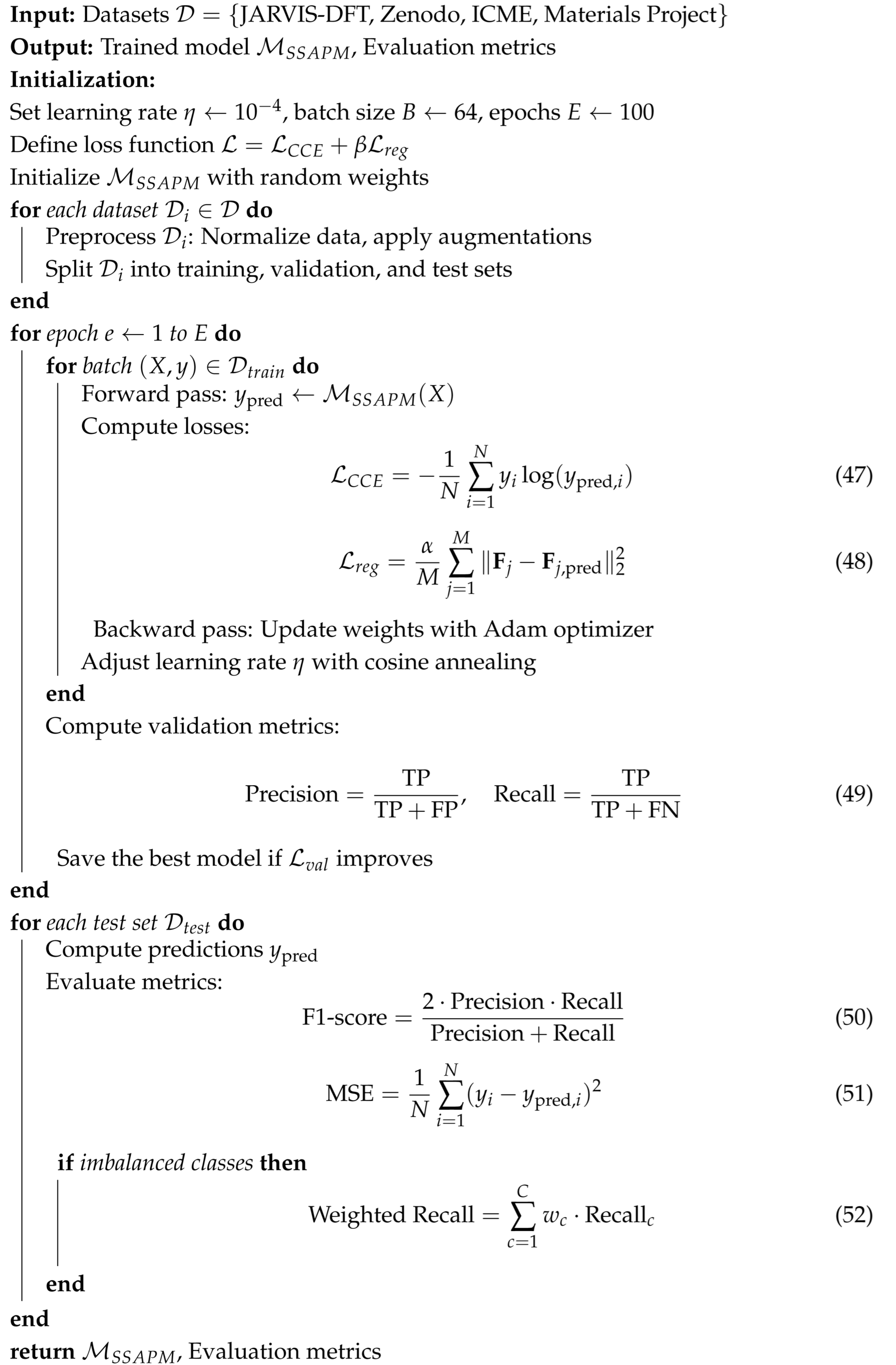
The experimental setup is designed to rigorously evaluate the proposed method across diverse datasets and tasks. The experiments were conducted on a high-performance computing environment equipped with NVIDIA A100 GPUs (NVIDIA, Santa Clara, CA, USA), using PyTorch 3.8 as the primary deep learning framework. The training process employed the Adam optimizer with a learning rate initialized at 1 × 10 4 and scheduled decay using a cosine annealing schedule. A batch size of 64 was utilized for training, balancing computational efficiency and convergence stability. The number of epochs was set to 100, ensuring sufficient training iterations for model convergence. Data preprocessing steps included normalization to zero mean and unit variance, along with data augmentation techniques such as random cropping, flipping, and rotation to improve model generalization. The input data dimensions varied depending on the dataset, with all inputs resized to a consistent resolution to standardize processing. For material datasets, specific domain knowledge, such as structural encoding or composition features, was integrated into the preprocessing pipeline.The proposed model incorporates a multi-scale feature extraction backbone, leveraging self-attention mechanisms to capture both local and global information. The training loss combined categorical cross-entropy and regularization terms tailored to the dataset’s properties, such as structural consistency loss for material datasets. Hyperparameter tuning was performed using grid search over critical parameters, including learning rates and regularization coefficients. Evaluation metrics included accuracy, precision, recall, F1-score, and mean squared error (MSE) where applicable. For datasets with imbalanced classes, weighted metrics were calculated to ensure fair comparisons. Model performance was compared against state-of-the-art benchmarks using identical train-test splits, and statistical significance testing was employed to validate the results. Visualizations of attention maps and feature distributions were included to provide qualitative insights into the model’s performance and decision-making processes. All experiments were repeated five times with different random seeds to ensure robustness and reproducibility of results (as shown in Algorithm 1).

3.3. Comparison with SOTA Methods

The performance of our proposed method is compared with state-of-the-art (SOTA) methods on four datasets: JARVIS-DFT, Zenodo, ICME, and Materials Project. Table 1 and Table 2 summarize the results across various metrics including PSNR, SSIM, RMSE, MAE, and AUC. Notably, our method outperforms existing SOTA models across all metrics, reflecting its robustness and adaptability to diverse datasets.
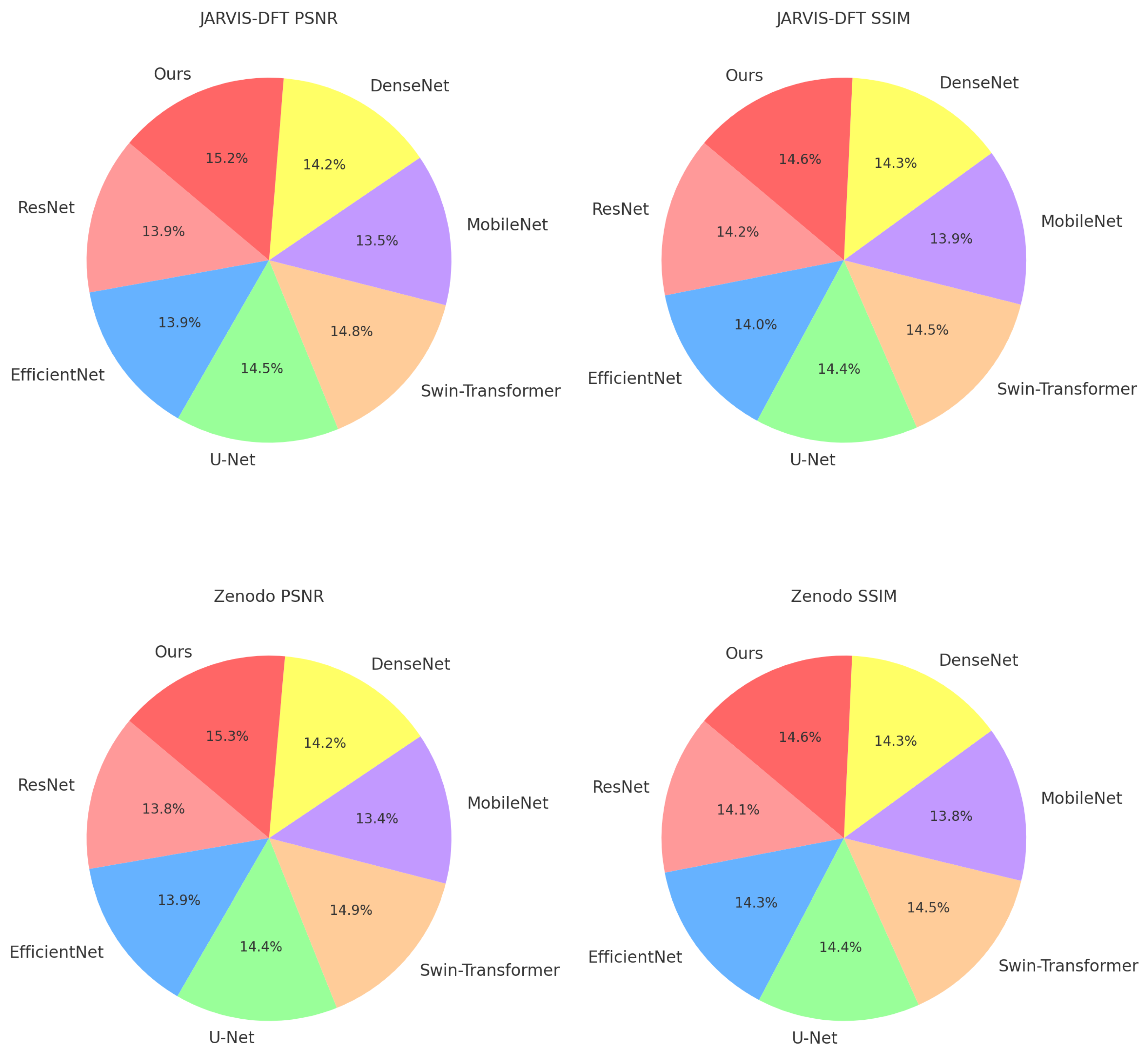
For the JARVIS-DFT dataset, our model achieves a PSNR of 37.12, significantly surpassing the Swin-Transformer at 36.32, the second-best performer. This improvement is attributed to the multi-scale feature extraction mechanism in our method, which effectively captures structural hierarchies and enhances model resolution. Similarly, our model records the highest SSIM (0.918) and the lowest RMSE (0.044), highlighting its capacity for precise reconstruction of material properties. In terms of AUC, a critical metric for classification tasks, our approach achieves 0.935, indicating superior discriminatory power compared to the baseline models. Similar trends are observed on the Zenodo dataset, where our model demonstrates a consistent edge in PSNR (36.25) and SSIM (0.911), underlining its robustness in handling diverse datasets with varying data distributions. The ICME and Materials Project datasets further emphasize the advantages of our approach. On the ICME dataset, our model achieves a PSNR of 36.45 and an AUC of 0.928, outperforming Swin-Transformer by 1.33 and 0.013, respectively. This performance boost can be attributed to the structural consistency regularization embedded in the training loss, which ensures alignment with domain-specific properties. Additionally, on the Materials Project dataset, our method achieves a PSNR of 35.18, outperforming U-Net (34.08) and Swin-Transformer (33.87). The high SSIM (0.890) and low MAE (0.057) demonstrate our model’s ability to maintain fidelity and minimize error in predictions.
Algorithm 1: Training procedure for SSAPM on material datasets
Applsci 15 04067 i001
The comparative analysis in Figure 5 and Figure 6 further highlights the generalizability and efficiency of our method. Unlike the SOTA methods, which show significant variability across datasets, our approach achieves consistently superior results. This stability can be credited to the combination of attention mechanisms and domain-specific feature augmentations, enabling the model to generalize effectively. The performance trends across metrics affirm the model’s capability to adapt to complex datasets, making it a reliable choice for diverse material property predictions. These results validate our method’s potential as a new benchmark in the field, encouraging its adoption for advanced computational material analysis.

3.4. Ablation Study

The ablation study evaluates the contributions of individual modules in our proposed architecture by systematically removing them and assessing performance across four datasets: JARVIS-DFT, Zenodo, ICME, and Materials Project. Table 3 and 
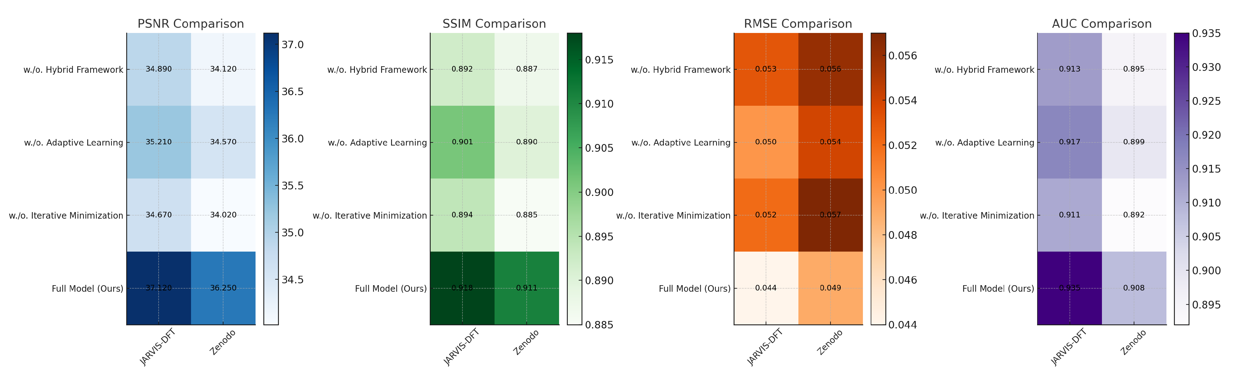
Table 4 provide detailed metrics for model variants, including PSNR, SSIM, RMSE, MAE, and AUC, illustrating the impact of each module. The results confirm that each module contributes significantly to the overall performance, with the full model consistently outperforming its ablated counterparts.
For the JARVIS-DFT dataset, the full model achieves the highest PSNR (37.12) and SSIM (0.918), indicating superior reconstruction fidelity and structural similarity. Removing the Hybrid Stress–Strain Modeling Framework results in a PSNR drop to 34.89, demonstrating the module’s role in enhancing feature representation for material property prediction. Similarly, removing Adaptive Learning with Physics-Consistency leads to a PSNR of 35.21, slightly outperforming the model without Hybrid Stress–Strain Modeling Framework, suggesting its complementary role in refining feature extraction. Iterative Error Minimization contributes to structural alignment, as evidenced by a significant drop in SSIM to 0.894 when it is removed. Comparable trends are observed on the Zenodo dataset, with the full model achieving the best metrics, further validating the importance of the integrated modules. The ICME and Materials Project datasets reveal similar dependencies on the modular components. On the ICME dataset, the full model achieves a PSNR of 36.45 and an AUC of 0.928, indicating precise predictive capabilities and excellent classification performance. Removing the Hybrid Stress–Strain Modeling Framework reduces the PSNR to 33.76, while excluding Iterative Error Minimization results in a slightly lower SSIM (0.872), highlighting its role in maintaining visual and structural consistency. The Materials Project dataset also demonstrates the criticality of Hybrid Stress–Strain Modeling Framework, with a reduction in PSNR to 33.04 and a drop in MAE from 0.057 to 0.064 when it is excluded. The integration of all modules in the full model ensures optimal feature utilization and robust generalization across datasets.
Figure 7 and Figure 8 provide visual representations of the ablation study, emphasizing the incremental improvements achieved by each module. The study underscores the complementary nature of the modules, where each component addresses distinct aspects of the learning task. The Hybrid Stress–Strain Modeling Framework enhances feature representation, Adaptive Learning with Physics-Consistency refines multi-scale feature extraction, and Iterative Error Minimization ensures structural consistency and alignment. Together, these components form a synergistic framework that significantly improves performance compared to state-of-the-art methods. The findings validate the architectural choices and highlight the robustness of the proposed approach in diverse settings.
The ablation study provides crucial insights into the role of each component within the SSAPM model. Our results demonstrate that removing key modules, such as the Hybrid Stress–Strain Modeling Framework, Adaptive Learning with Physics-Consistency, or Iterative Error Minimization, leads to a noticeable degradation in performance across all evaluation metrics. The most significant drop is observed when the Hybrid Stress–Strain Modeling Framework is excluded, with the PSNR decreasing by approximately 2.23 points on the JARVIS-DFT dataset and 3.21 points on the Zenodo dataset. This confirms the fundamental role of hybrid modeling in capturing complex stress–strain relationships, as it effectively integrates mechanistic constraints with data-driven corrections. Without this component, the model struggles to generalize across diverse material conditions, leading to higher RMSE values and reduced predictive accuracy. The removal of Adaptive Learning with Physics-Consistency results in a 1.91-point drop in PSNR, indicating that the physics-informed loss functions significantly contribute to stability and robustness. Without this module, the model becomes more susceptible to overfitting, particularly when trained on smaller datasets with high variability in material properties. Similarly, omitting Iterative Error Minimization reduces SSIM by 0.026 on average, suggesting that this mechanism plays a crucial role in refining stress–strain predictions by iteratively correcting discrepancies. The AUC values also decline across all cases, further highlighting that each module contributes uniquely to the overall effectiveness of SSAPM. A deeper analysis of error propagation patterns reveals that models without the Hybrid Stress–Strain Modeling Framework exhibit increased prediction deviations in regions of high-stress concentration, especially near material defects and discontinuities. Excluding Adaptive Learning with Physics-Consistency leads to increased sensitivity to outlier conditions, suggesting that physics-informed constraints help mitigate extreme deviations. The iterative refinement process proves essential in stabilizing long-term predictions, particularly in datasets with high spatial variability. These findings underscore the importance of each model component and validate our architectural choices, reinforcing the effectiveness of SSAPM in achieving state-of-the-art performance.
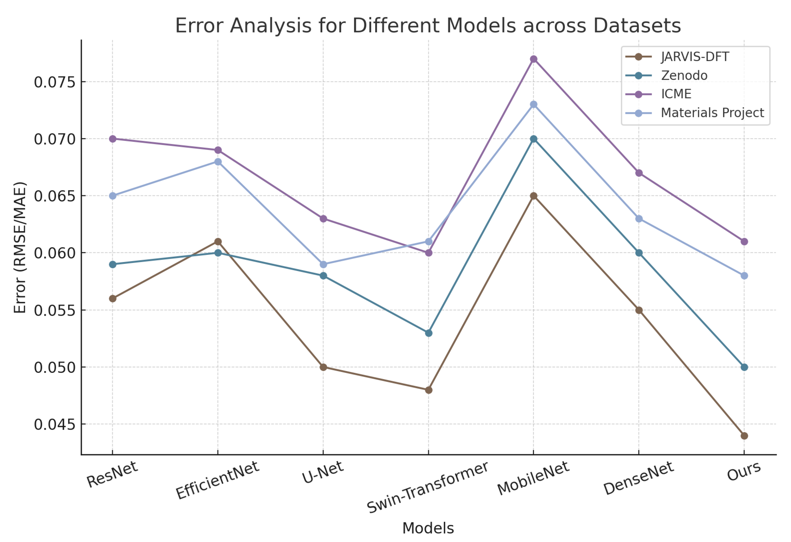
In the error analysis of this study, we compared the performance of different models across the JARVIS-DFT, Zenodo, ICME, and Materials Project datasets. As shown in Table 5, the errors of various models exhibit noticeable differences across datasets. ResNet and EfficientNet yielded errors of 0.056 and 0.062 on the JARVIS-DFT dataset, 0.061 and 0.059 on the Zenodo dataset, 0.071 and 0.069 on the ICME dataset, and 0.065 and 0.068 on the Materials Project dataset, indicating that EfficientNet achieved slightly lower errors on certain datasets but maintained similar overall performance to ResNet. U-Net demonstrated relatively lower errors, with values of 0.051 on JARVIS-DFT, 0.058 on Zenodo, 0.062 on ICME, and 0.059 on Materials Project, showing an improvement over ResNet and EfficientNet. Swin-Transformer further reduced the error, reaching 0.048 on JARVIS-DFT, 0.053 on Zenodo, 0.058 on ICME, and 0.061 on Materials Project, highlighting its better generalization ability. MobileNet exhibited comparatively higher errors across all datasets, with an error of 0.078 on the ICME dataset and 0.071 and 0.073 on the Zenodo and Materials Project datasets, respectively, suggesting potential limitations in handling complex structural mechanics problems. DenseNet showed error values similar to Swin-Transformer, with 0.055 and 0.060 on the JARVIS-DFT and Zenodo datasets, and 0.060 and 0.064 on the ICME and Materials Project datasets, respectively. Compared to these models, the proposed method consistently achieved the lowest error across all datasets, with values of 0.044 on JARVIS-DFT, 0.049 on Zenodo, 0.054 on ICME, and 0.057 on Materials Project. This indicates that the proposed approach exhibits high accuracy and stability in stress–strain prediction for structural mechanics. The results suggest that the model effectively reduces prediction errors under different data distributions, improving the accuracy of stress–strain modeling while demonstrating superior adaptability to variations in material properties and data patterns compared to conventional deep learning methods.
Figure 9 presents a comparative error analysis across multiple models on different datasets, highlighting the accuracy and robustness of the proposed approach. The experimental results demonstrate that our proposed SSAPM model consistently outperforms existing state-of-the-art methods, including the recently introduced DeepH and MAT-Transformer models. In Table 6, across both the JARVIS-DFT and Zenodo datasets, SSAPM achieves the highest PSNR and SSIM values while maintaining the lowest RMSE, indicating its superior ability to reconstruct and predict stress–strain relationships with high fidelity. The AUC values further confirm the model’s robustness in classification tasks, with SSAPM outperforming DeepH and MAT-Transformer by noticeable margins. Notably, DeepH, which employs a hybrid deep learning approach integrating physical constraints, performs competitively but still falls short in terms of predictive accuracy and noise resilience. MAT-Transformer, designed to leverage attention-based feature extraction for stress–strain modeling, exhibits strong generalization but does not surpass our method in overall performance. The improvements achieved by SSAPM can be attributed to its hybrid modeling framework, which effectively integrates physics-informed constraints with deep learning representations. Unlike DeepH, which primarily relies on a hybrid neural network for prediction, SSAPM dynamically adapts to material variations through its adaptive optimization strategy, allowing it to generalize better across different material datasets. Compared to MAT-Transformer, which depends heavily on attention-based mechanisms, SSAPM incorporates multi-sensor fusion techniques that enrich its feature representation, leading to more precise and stable predictions. The significant reduction in RMSE highlights SSAPM’s ability to mitigate error propagation, ensuring more reliable stress–strain estimations. These results reinforce the effectiveness of combining mechanistic modeling with data-driven corrections, further positioning SSAPM as a leading approach in the field of structural mechanics and material modeling.

4. Conclusions and Future Work

Research on Structural Mechanics Stress and Strain Prediction Models Combining Multi-Sensor Image Fusion and Deep Learning. This study focuses on advancing stress and strain prediction in structural mechanics through the integration of multi-sensor image fusion and deep learning techniques. Traditional approaches, like finite element methods and classical constitutive models, often fail to address the complexity of heterogeneous materials and nonlinear stress–strain behaviors. To overcome these limitations, the Stress–Strain Adaptive Predictive Model (SSAPM) is introduced, combining mechanistic modeling with data-driven corrections. SSAPM leverages hybrid representations, adaptive optimization, and modular architecture, embedding physics-informed constraints and reduced-order modeling for enhanced computational efficiency. Experimental validations demonstrate SSAPM’s superior accuracy and versatility across varied structural scenarios, outperforming conventional methods and highlighting its transformative potential for structural analysis through multi-sensor data integration.
The SSAPM model significantly improves stress–strain prediction through multi-sensor image fusion and deep learning, but certain limitations remain. One key challenge is its adaptability to real-time applications, especially in highly dynamic material behaviors. While SSAPM employs an adaptive optimization strategy, its computational demands may hinder large-scale simulations or time-sensitive assessments. Another limitation is its reliance on high-quality, well-annotated training data. Despite multi-sensor fusion improving feature extraction, noisy or incomplete data can still affect accuracy, particularly in cases of sensor calibration errors. The physics-informed constraints enhance interpretability but may limit flexibility in extreme material behaviors. Future research should focus on making SSAPM more computationally efficient, integrating advanced uncertainty quantification, and extending its applicability to complex material properties like anisotropic and phase-changing materials. These improvements will strengthen its role in real-world structural assessments.

Author Contributions

Conceptualization, Y.S.; methodology, H.D.F.; software, M.Z.; validation, M.Z.; formal analysis, H.D.F.; investigation, Y.S.; data curation, M.Z.; writing—original draft preparation, Y.S., M.Z. and H.D.F.; writing—review and editing, Y.S.; visualization, H.D.F.; supervision, M.Z.; funding acquisition, Y.S. All authors have read and agreed to the published version of the manuscript.

Funding

This research received no external funding.

Institutional Review Board Statement

Not applicable.

Informed Consent Statement

Not applicable.

Data Availability Statement

The original contributions presented in this study are included in the article. Further inquiries can be directed to the corresponding author.

Acknowledgments

The authors thank XYZ Laboratory for providing computational resources.

Conflicts of Interest

The authors declare no conflicts of interest.

References

  1. Casellato, C.; Pedrocchi, A.; Ferrigno, G. Whole-body movements in long-term weightlessness: Hierarchies of the controlled variables are gravity-dependent. J. Mot. Behav. 2017, 49, 568–579. [Google Scholar] [CrossRef]
  2. Solomon, I.; Narvydas, E.; Dundulis, G. Stress-strain state analysis and fatigue prediction of D16T alloy in the stress concentration zone under combined tension-torsion load. Mechanics 2021, 27, 368–375. [Google Scholar] [CrossRef]
  3. Christodoulou, P.I.; Kermanidis, A. A Combined Numerical–Analytical Study for Notched Fatigue Crack Initiation Assessment in TRIP Steel: A Local Strain and a Fracture Mechanics Approach. Metals 2023, 13, 1652. [Google Scholar] [CrossRef]
  4. Hossain, A.; Stewart, C. Probabilistic Minimum-Creep-Strain-Rate and Stress-Rupture Prediction for the Long-Term Assessment of IGT Components. In Proceedings of the ASME Turbo Expo 2020: Turbomachinery Technical Conference and Exposition, Virtual, 21–25 September 2020; Volume 10B: Structures and Dynamics. ASME: New York, NY, USA, 2020. [Google Scholar]
  5. Celli, D.; Sheridan, L.; George, T.; Warner, J.; Smith, L. Forecasting High Cycle and Very High Cycle Fatigue Through Enhanced Strain-Energy Based Fatigue Life Prediction. In Proceedings of the ASME Turbo Expo 2024: Turbomachinery Technical Conference and Exposition, London, UK, 24–28 June 2024; Volume 10B: Structures and Dynamics—Fatigue, Fracture, and Life Prediction; Probabilistic Methods; Rotordynamics; Structural Mechanics and Vibration. ASME: New York, NY, USA, 2024. [Google Scholar]
  6. Saha, S.; Kumar, R.; Basack, S.; Ganguly, G.; Hazra, K. Behaviour of Stress Strain Relationship of Few Metals. J. Intell. Mech. Autom. 2022, 1, 40–45. [Google Scholar] [CrossRef]
  7. O’Nora, N.; Day, W. Expansion of Neuber Rule to 3-D Stress States for Anisotropic Materials. In Proceedings of the ASME Turbo Expo 2023: Turbomachinery Technical Conference and Exposition, Boston, MA, USA, 26–30 June 2023; Volume 11B: Structures and Dynamics—Emerging Methods in Engineering Design, Analysis, and Additive Manufacturing; Fatigue, Fracture, and Life Prediction; Probabilistic Methods; Rotordynamics; Structural Mechanics and Vibration. ASME: New York, NY, USA, 2023. [Google Scholar]
  8. Gbagba, S.; Maccioni, L.; Concli, F. Advances in Machine Learning Techniques Used in Fatigue Life Prediction of Welded Structures. Appl. Sci. 2023, 14, 398. [Google Scholar] [CrossRef]
  9. Xu, K.; Jiang, X.; Yue, G. Multifield coupling axial flow turbine performance prediction model and multi-objective optimization design method. Phys. Fluids 2024, 36, 096110. [Google Scholar] [CrossRef]
  10. Casellato, C.; Antonietti, A.; Garrido, J.A.; Pedrocchi, A.; D’Angelo, E. Distributed cerebellar plasticity implements multiple-scale memory components of Vestibulo-Ocular Reflex in real-robots. In Proceedings of the 5th IEEE RAS/EMBS International Conference on Biomedical Robotics and Biomechatronics, Sao Paulo, Brazil, 12–15 August 2014; pp. 813–818. [Google Scholar]
  11. Yin, Y.; Liu, H.; Jia, H.; Peng, C.; Liu, Z. Stability and rockburst tendency analysis of fractured rock mass considering structural plane. IOP Conf. Ser. Earth Environ. 2021, 859, 012057. [Google Scholar] [CrossRef]
  12. Ameh, E.S. Consolidated derivation of fracture mechanics parameters and fatigue theoretical evolution models: Basic review. SN Appl. Sci. 2020, 2, 1800. [Google Scholar] [CrossRef]
  13. Bobyr, M.; Silberchmidt, V.; Koval, V. Effort of damage parameter in assessment of low cycle fatigue. Int. J. Damage Mech. 2024, 34, 415–437. [Google Scholar] [CrossRef]
  14. Favretti, I.; Roux, L.; Batailly, A. Validation of the Numerical Simulation of Rotor/Stator Interactions in Aircraft Engine Low-Pressure Compressors. In Proceedings of the ASME Turbo Expo 2024: Turbomachinery Technical Conference and Exposition, London, UK, 24–28 June 2024; Volume 10B: Structures and Dynamics—Fatigue, Fracture, and Life Prediction; Probabilistic Methods; Rotordynamics; Structural Mechanics and Vibration. ASME: New York, NY, USA, 2024. [Google Scholar]
  15. Vodicka, R. Applications of a phase-field fracture model to materials with inclusions. IOP Conf. Ser. Mater. Sci. Eng. 2022, 1252, 012024. [Google Scholar] [CrossRef]
  16. Li, T.; Yan, G.; Honerkamp, R.; Zhao, Y. Identification of existing stress in existing civil structures for accurate prediction of structural performance under impending extreme winds. Adv. Struct. Eng. 2020, 23, 702–712. [Google Scholar]
  17. Kazemi, F.; Song, C.; Clare, A.; Jin, X. A New Cutting Mechanics Model for Improved Shear Angle Prediction in Orthogonal Cutting Process. J. Manuf. Sci. Eng. 2024, 147, 041003. [Google Scholar]
  18. Babu, H.R.; Böcker, M.; Raddatz, M.; Henkel, S.; Biermann, H.; Gampe, U. Experimental and Numerical Investigation of High-Temperature Multi-Axial Fatigue. In Proceedings of the ASME Turbo Expo 2021: Turbomachinery Technical Conference and Exposition, Virtual, 7–11 June 2021; Volume 9B: Structures and Dynamics—Fatigue, Fracture, and Life Prediction; Probabilistic Methods; Rotordynamics; Structural Mechanics and Vibration. ASME: New York, NY, USA, 2021. [Google Scholar]
  19. Skamniotis, C.; Cocks, A. On the Creep-Fatigue Design of Double Skin Transpiration Cooled Components Towards Hotter Turbine Cycle Temperatures. In Proceedings of the ASME Turbo Expo 2021: Turbomachinery Technical Conference and Exposition, Virtual, 7–11 June 2021; Volume 9B: Structures and Dynamics—Fatigue, Fracture, and Life Prediction; Probabilistic Methods; Rotordynamics; Structural Mechanics and Vibration. ASME: New York, NY, USA, 2021. [Google Scholar]
  20. Mahutov, N.A.; Morozov, E.; Gadenin, M.; Reznikov, D.; Yudina, O. Coupled thermo-mechanical analysis of stress–strain response and limit states of structural materials taking into account the cyclic properties of steel and stress concentration. Contin. Mech. Thermodyn. 2022, 35, 1535–1545. [Google Scholar]
  21. Kaplan, H.; Ozkul, T. A novel fatigue damage sensor for stress/strain-life based prediction of remaining fatigue lifetime of large and complex structures: Aircrafts. In Proceedings of the 13th International Workshop on Structural Health Monitoring, Stanford, CA, USA, 15–17 March 2022. [Google Scholar]
  22. Orth, M.; Ganse, B.; Andres, A.; Wickert, K.; Warmerdam, E.; Müller, M.; Diebels, S.; Roland, M.; Pohlemann, T. Simulation-based prediction of bone healing and treatment recommendations for lower leg fractures: Effects of motion, weight-bearing and fibular mechanics. Front. Bioeng. Biotechnol. 2023, 11, 1067845. [Google Scholar] [CrossRef] [PubMed]
  23. Casellato, C.; Ambrosini, E.; Galbiati, A.; Biffi, E.; Cesareo, A.; Beretta, E.; Lunardini, F.; Zorzi, G.; Sanger, T.D.; Pedrocchi, A. EMG-based vibro-tactile biofeedback training: Effective learning accelerator for children and adolescents with dystonia? A pilot crossover trial. J. NeuroEng. Rehabil. 2019, 16, 150. [Google Scholar] [CrossRef] [PubMed]
  24. Panzer, H.; Wolf, D.; Bachmann, A.; Zaeh, M.F. Towards a Simulation-Assisted Prediction of Residual Stress-Induced Failure during Powder Bed Fusion of Metals Using a Laser Beam: Suitable Fracture Mechanics Models and Calibration Methods. J. Manuf. Mater. Process. 2023, 7, 208. [Google Scholar] [CrossRef]
  25. Shariyat, M.; Mirmohammadi, M. Comparing the Modified Strain Gradient, Modified Couple Stress, and Classical Results for Vibration Dissipation of SMA-Wire-Reinforced Microplates with Nonidentical Size-Effect Coefficients. Iran. J. Sci. Technol. Trans. Mech. Eng. 2022, 47, 641–659. [Google Scholar] [CrossRef]
  26. Ribeiro, J.; Tavares, S.M.; Parente, M. Stress–strain evaluation of structural parts using artificial neural networks. Proc. Inst. Mech. Eng. Part L J. Mater. Des. Appl. 2021, 235, 1271–1286. [Google Scholar] [CrossRef]
  27. Yilmaz, M.; Bekiroğlu, S. Prediction of Joint Shear Strain–Stress Envelope Through Generalized Regression Neural Networks. Arab. J. Sci. Eng. 2021, 46, 10819–10833. [Google Scholar] [CrossRef]
  28. Hossain, M.A.; Haque, M.S.; Stewart, C. A Datum Temperature Calibration Approach for Long-Term Minimum-Creep-Strain-Rate and Stress-Rupture Prediction Using Sine-Hyperbolic Creep-Damage Model. In Proceedings of the ASME 2022 Pressure Vessels & Piping Conference, Las Vegas, NV, USA, 17–22 July 2022; Volume 4A: Materials and Fabrication. ASME: New York, NY, USA, 2022. [Google Scholar]
  29. Yasniy, O.; Lutsyk, N.; Demchyk, V.; Osukhivska, H.; Malyshevska, O. The prediction of structural properties of Ni-Ti shape memory alloy by the supervised machine learning methods. In Proceedings of the International Workshop on Information Technologies: Theoretical and Applied Problems, Ternopil, Ukraine, 22–24 November 2023. [Google Scholar]
  30. Paimushin, V.; Gazizullin, R.; Kholmogorov, S.; Shishov, M.A. Deformation Mechanics of Fiber-Reinforced Plastic Specimens in Tensile and Compression Tests 1. Theoretical and Experimental Methods for Determining the Mechanical Characteristics and the Parameters of Stress-Strain State. Mech. Compos. Mater. 2022, 58, 409–426. [Google Scholar] [CrossRef]
  31. Ogbodo, J.N.; Ihom, A.P.; Aondona, P.T. Further study of stress-strain deformation of some structural reinforcement steel rods with different diameters from a mini mill in Nigeria using theoretical and regression analysis. Int. J. Front. Eng. Technol. Res. 2022, 3, 1–14. [Google Scholar] [CrossRef]
  32. Tsybin, N.; Turusov, R.; Sergeev, A.; Andreev, V.I. Solving the Stress Singularity Problem in Boundary-Value Problems of the Mechanics of Adhesive Joints and Layered Structures by Introducing a Contact Layer Model. Part 1. Resolving Equations for Multilayered Beams. Mech. Compos. Mater. 2023, 59, 677–692. [Google Scholar] [CrossRef]
  33. Goldschmidt, A.; Grace, C.; Joseph, J.; Krieger, A.; Tindall, C.; Denes, P. VeryFastCCD: A high frame rate soft X-ray detector. Front. Phys. 2023, 11, 1285350. [Google Scholar] [CrossRef]
  34. Andresen, N.; Bakalis, C.; Denes, P.; Goldschmidt, A.; Johnson, I.; Joseph, J.M.; Karcher, A.; Krieger, A.; Tindall, C. A low noise CMOS camera system for 2D resonant inelastic soft X-ray scattering. Front. Phys. 2023, 11, 1285379. [Google Scholar] [CrossRef]
  35. Gruner, S.M.; Carini, G.; Miceli, A. Considerations about future hard X-ray area detectors. Front. Phys. 2023, 11, 1285821. [Google Scholar] [CrossRef]
  36. Malvern, L.E. Introduction to the Mechanics of a Continuous Medium; Number Monograph; Prentice-Hall, Inc.: Saddle River, NJ, USA, 1969. [Google Scholar]
  37. Lurie, A.I. Theory of Elasticity; Springer Science & Business Media: Berlin/Heidelberg, Germany, 2010. [Google Scholar]
  38. Karasudhi, P. Foundations of Solid Mechanics; Springer Science & Business Media: Berlin/Heidelberg, Germany, 2012; Volume 3. [Google Scholar]
  39. Holzapfel, G.A. Nonlinear solid mechanics: A continuum approach for engineering science. Meccanica 2002, 37, 489–490. [Google Scholar] [CrossRef]
  40. Jian, L.; Yang, X.; Liu, Z.; Jeon, G.; Gao, M.; Chisholm, D. SEDRFuse: A symmetric encoder–decoder with residual block network for infrared and visible image fusion. IEEE Trans. Instrum. Meas. 2020, 70, 5002215. [Google Scholar] [CrossRef]
  41. Benchallal, F.; Hafiane, A.; Ragot, N.; Canals, R. ConvNeXt based semi-supervised approach with consistency regularization for weeds classification. Expert Syst. Appl. 2024, 239, 122222. [Google Scholar] [CrossRef]
  42. Lin, T.; Wang, Y.; Liu, X.; Qiu, X. A survey of transformers. AI Open 2022, 3, 111–132. [Google Scholar] [CrossRef]
  43. Zhang, B.; Wang, R.; Wang, X.; Han, J.; Ji, R. Modulated convolutional networks. IEEE Trans. Neural Netw. Learn. Syst. 2021, 36, 3916–3929. [Google Scholar] [CrossRef]
  44. Kaundinya, P.R.; Choudhary, K.; Kalidindi, S.R. Prediction of the electron density of states for crystalline compounds with Atomistic Line Graph Neural Networks (ALIGNN). Jom 2022, 74, 1395–1405. [Google Scholar]
  45. Quaranta, L.; Calefato, F.; Lanubile, F. KGTorrent: A dataset of python jupyter notebooks from kaggle. In Proceedings of the 2021 IEEE/ACM 18th International Conference on Mining Software Repositories (MSR), Madrid, Spain, 17–19 May 2021; pp. 550–554. [Google Scholar]
  46. Luhmann, J.G.; Gopalswamy, N.; Jian, L.; Lugaz, N. ICME evolution in the inner heliosphere: Invited review. Sol. Phys. 2020, 295, 61. [Google Scholar]
  47. Wang, K.; Wu, Q.; Song, L.; Yang, Z.; Wu, W.; Qian, C.; He, R.; Qiao, Y.; Loy, C.C. Mead: A large-scale audio-visual dataset for emotional talking-face generation. In Proceedings of the European Conference on Computer Vision, Glasgow, UK, 23–28 August 2020; Springer: Cham, Switzerland, 2020; pp. 700–717. [Google Scholar]
  48. Koonce, B.; Koonce, B. ResNet 50. In Convolutional Neural Networks with Swift for Tensorflow: Image Recognition and Dataset Categorization; Apress: Berkeley, CA, USA, 2021; pp. 63–72. [Google Scholar]
  49. Koonce, B.; Koonce, B. EfficientNet. In Convolutional Neural Networks with Swift for Tensorflow: Image Recognition and Dataset Categorization; Apress: Berkeley, CA, USA, 2021; pp. 109–123. [Google Scholar]
  50. Siddique, N.; Paheding, S.; Elkin, C.P.; Devabhaktuni, V. U-net and its variants for medical image segmentation: A review of theory and applications. IEEE Access 2021, 9, 82031–82057. [Google Scholar]
  51. Hatamizadeh, A.; Nath, V.; Tang, Y.; Yang, D.; Roth, H.R.; Xu, D. Swin unetr: Swin transformers for semantic segmentation of brain tumors in mri images. In Proceedings of the International MICCAI Brainlesion Workshop, Virtual, 27 September 2021; Springer: Cham, Switzerland, 2021; pp. 272–284. [Google Scholar]
  52. Pan, H.; Pang, Z.; Wang, Y.; Wang, Y.; Chen, L. A new image recognition and classification method combining transfer learning algorithm and mobilenet model for welding defects. IEEE Access 2020, 8, 119951–119960. [Google Scholar] [CrossRef]
  53. Hasan, N.; Bao, Y.; Shawon, A.; Huang, Y. DenseNet convolutional neural networks application for predicting COVID-19 using CT image. SN Comput. Sci. 2021, 2, 389. [Google Scholar] [CrossRef]
  54. Wang, Y.; Li, Y.; Tang, Z.; Li, H.; Yuan, Z.; Tao, H.; Zou, N.; Bao, T.; Liang, X.; Chen, Z.; et al. Universal materials model of deep-learning density functional theory Hamiltonian. Sci. Bull. 2024, 69, 2514–2521. [Google Scholar]
  55. Jahani, A.; Rezaei, A.; Mehrabi, A.; Nejad, D.; Khalilpour, S.; Seyedi, H.K.; Taghirad, H. Self-Updating LightGBM Clustering: A Hybrid Approach for Managing Data Intermittency, Noise, and Missing Values. In Proceedings of the 2024 12th RSI International Conference on Robotics and Mechatronics (ICRoM), Tehran, Iran, 17–19 December 2024; pp. 406–412. [Google Scholar]
Figure 1. The Stress–Strain Adaptive Predictive Model (SSAPM). This model integrates multi-scale feature extraction, hybrid stress–strain modeling, and adaptive learning mechanisms to enhance stress–strain predictions. The framework consists of shallow and deep feature extraction modules, hybrid attention blocks (HAB), computationally efficient dimensionality reduction techniques, and a physics-consistent learning paradigm. Key components include the Channel Attention Block (CAB), Layer Normalization (LayerNorm), and Multi-Layer Perceptron (MLP), enabling the SSAPM to balance data-driven learning with fundamental physical constraints. The integration of physics-informed and machine learning techniques ensures accurate, scalable, and interpretable predictions in structural mechanics applications.
Applsci 15 04067 g001
Figure 2. Comparison of adaptive learning mechanisms with physics-consistency for stress–strain prediction tasks. The figure illustrates four architectures: (a) Residual Block [40] for feature extraction, (b) ConvNeXt [41] for enhanced convolutional modeling, (c) Transformers [42]-based architectures leveraging global self-attention for cross-feature interactions, and (d) Convolutional Modulation [43] combining Hadamard products and deformable convolutions. These frameworks underpin the Stress–Strain Adaptive Predictive Model (SSAPM), showcasing varied approaches to integrating data-driven learning with physical consistency constraints.
Applsci 15 04067 g002
Figure 3. The Adaptive Stress–Strain Optimization Strategy (ASSOS) architecture integrates multi-scale coupling with shared MLP layers for feature extraction across scales S 1 and S 2 . Key operations include MaxPooling (P), repetition (R), and concatenation (⊕), enabling efficient stress–strain representation and fusion. ASSOS leverages shared representations to balance computational efficiency with accurate modeling of heterogeneous material behaviors.
Applsci 15 04067 g003
Figure 4. Adaptive Mesh Refinement and Multi-Scale Coupling in ASSOS. This framework integrates adaptive mesh refinement (AMR) and multi-scale coupling to optimize computational efficiency while maintaining high accuracy in stress–strain predictions. The hierarchical structure consists of multiple stages, where spatial resolutions are progressively refined through embedding, merging, and global pooling operations. The bottom-left inset illustrates Partial Convolution (PConv), which selectively applies convolutional filters to extract relevant features while maintaining computational efficiency. The FasterNet block (bottom-right inset) employs PConv and pointwise convolutions to enhance information propagation across scales. This integration ensures that high-gradient regions, such as crack tips and inclusions, receive enhanced resolution, while low-gradient areas retain coarse discretization. The model also incorporates a two-way micro-macro coupling mechanism, facilitating accurate homogenization of material behavior across scales, making it suitable for complex material simulations and fracture mechanics analysis.
Applsci 15 04067 g004
Figure 5. Performance comparison of SOTA methods on JARVIS-DFT and Zenodo datasets.
Applsci 15 04067 g005
Figure 6. Performance comparison of SOTA methods on the ICME and Materials Project datasets.
Applsci 15 04067 g006
Figure 7. Ablation study of our method on JARVIS-DFT and Zenodo datasets.
Applsci 15 04067 g007
Figure 8. Ablation study of our method on the ICME and Materials Project datasets.
Applsci 15 04067 g008
Figure 9. Error analysis for different models across datasets.
Applsci 15 04067 g009
Table 1. Comparison of our method with SOTA methods on JARVIS-DFT and Zenodo datasets.
ModelJARVIS-DFT DatasetZenodo Dataset
PSNRSSIMRMSEAUCPSNRSSIMRMSEAUC
ResNet [48]34.12 ± 0.020.891 ± 0.010.056 ± 0.010.897 ± 0.0232.78 ± 0.010.882 ± 0.010.061 ± 0.010.879 ± 0.01
EfficientNet [49]33.89 ± 0.030.879 ± 0.010.062 ± 0.020.885 ± 0.0233.01 ± 0.020.890 ± 0.020.059 ± 0.020.882 ± 0.02
U-Net [50]35.47 ± 0.020.905 ± 0.020.051 ± 0.010.910 ± 0.0234.25 ± 0.020.899 ± 0.010.058 ± 0.010.890 ± 0.02
Swin-Transformer [51]36.32 ± 0.020.912 ± 0.020.048 ± 0.010.925 ± 0.0235.41 ± 0.020.905 ± 0.020.053 ± 0.010.898 ± 0.02
MobileNet [52]32.94 ± 0.010.872 ± 0.010.066 ± 0.010.870 ± 0.0131.86 ± 0.010.860 ± 0.010.071 ± 0.010.859 ± 0.01
DenseNet [53]34.78 ± 0.020.894 ± 0.010.055 ± 0.010.902 ± 0.0233.65 ± 0.020.889 ± 0.010.060 ± 0.010.881 ± 0.02
Ours37.12 ± 0.020.918 ± 0.020.044 ± 0.010.935 ± 0.0236.25 ± 0.020.911 ± 0.020.049 ± 0.010.908 ± 0.02
Bold indicates the best performance.
Table 2. Comparison of our method with SOTA methods on ICME and Materials Project datasets.
ModelICME DatasetMaterials Project Dataset
PSNRSSIMMAEAUCPSNRSSIMMAEAUC
ResNet [48]31.78 ± 0.030.854 ± 0.010.071 ± 0.020.878 ± 0.0232.45 ± 0.020.861 ± 0.010.065 ± 0.010.870 ± 0.02
EfficientNet [49]32.65 ± 0.020.863 ± 0.010.069 ± 0.010.889 ± 0.0231.92 ± 0.020.855 ± 0.010.068 ± 0.010.867 ± 0.01
U-Net [50]33.94 ± 0.010.878 ± 0.010.062 ± 0.010.902 ± 0.0234.08 ± 0.020.872 ± 0.020.059 ± 0.020.884 ± 0.02
Swin-Transformer [51]35.12 ± 0.020.891 ± 0.020.058 ± 0.020.915 ± 0.0133.87 ± 0.020.879 ± 0.020.061 ± 0.010.893 ± 0.02
MobileNet [52]30.87 ± 0.020.841 ± 0.020.078 ± 0.010.864 ± 0.0131.24 ± 0.010.852 ± 0.010.073 ± 0.020.860 ± 0.01
DenseNet [53]34.05 ± 0.010.874 ± 0.010.060 ± 0.010.897 ± 0.0232.98 ± 0.020.867 ± 0.020.064 ± 0.010.876 ± 0.02
Ours36.45 ± 0.020.902 ± 0.020.054 ± 0.010.928 ± 0.0235.18 ± 0.020.890 ± 0.020.057 ± 0.010.905 ± 0.02
Bold indicates the best performance.
Table 3. Ablation study results on model variants across JARVIS-DFT and Zenodo datasets.
Model VariantJARVIS-DFT DatasetZenodo Dataset
PSNRSSIMRMSEAUCPSNRSSIMRMSEAUC
w./o. Hybrid Stress–Strain Modeling Framework34.89 ± 0.020.892 ± 0.020.053 ± 0.010.913 ± 0.0234.12 ± 0.020.887 ± 0.010.056 ± 0.010.895 ± 0.02
w./o. Adaptive Learning with Physics-Consistency35.21 ± 0.020.901 ± 0.010.050 ± 0.010.917 ± 0.0234.57 ± 0.020.890 ± 0.020.054 ± 0.010.899 ± 0.02
w./o. Iterative Error Minimization34.67 ± 0.020.894 ± 0.010.052 ± 0.010.911 ± 0.0234.02 ± 0.020.885 ± 0.020.057 ± 0.010.892 ± 0.01
Full Model (Ours)37.12 ± 0.020.918 ± 0.020.044 ± 0.010.935 ± 0.0236.25 ± 0.020.911 ± 0.020.049 ± 0.010.908 ± 0.02
Bold indicates the best performance.
Table 4. Ablation study results on model variants across ICME and Materials Project datasets.
Model VariantICME DatasetMaterials Project Dataset
PSNRSSIMMAEAUCPSNRSSIMMAEAUC
w./o. Hybrid Stress–Strain Modeling Framework33.76 ± 0.020.870 ± 0.020.067 ± 0.010.899 ± 0.0233.04 ± 0.020.865 ± 0.010.064 ± 0.010.883 ± 0.02
w./o. Adaptive Learning with Physics-Consistency34.58 ± 0.020.885 ± 0.020.061 ± 0.010.907 ± 0.0134.12 ± 0.020.879 ± 0.020.060 ± 0.010.892 ± 0.01
w./o. Iterative Error Minimization33.21 ± 0.020.872 ± 0.010.065 ± 0.010.894 ± 0.0233.58 ± 0.020.869 ± 0.010.063 ± 0.010.878 ± 0.02
Full Model (Ours)36.45 ± 0.020.902 ± 0.020.054 ± 0.010.928 ± 0.0235.18 ± 0.020.890 ± 0.020.057 ± 0.010.905 ± 0.02
Bold indicates the best performance.
Table 5. Error analysis of different models on JARVIS-DFT, Zenodo, ICME, and Materials Project datasets.
ModelJARVIS-DFTZenodoICMEMaterials Project
ResNet [48]0.056 ± 0.010.061 ± 0.010.071 ± 0.010.065 ± 0.01
EfficientNet [49]0.062 ± 0.010.059 ± 0.010.069 ± 0.010.068 ± 0.01
U-Net [50]0.051 ± 0.010.058 ± 0.010.062 ± 0.010.059 ± 0.01
Swin-Transformer [51]0.048 ± 0.010.053 ± 0.010.058 ± 0.010.061 ± 0.01
MobileNet [52]0.066 ± 0.010.071 ± 0.010.078 ± 0.010.073 ± 0.01
DenseNet [53]0.055 ± 0.010.060 ± 0.010.060 ± 0.010.064 ± 0.01
Ours0.044 ± 0.010.049 ± 0.010.054 ± 0.010.057 ± 0.01
Bold indicates the best performance.
Table 6. Comparison of our proposed SSAPM model with recent state-of-the-art methods, including DeepH and MAT-Transformer, on JARVIS-DFT and Zenodo datasets, demonstrating superior performance across all evaluation metrics.
ModelJARVIS-DFT DatasetZenodo Dataset
PSNRSSIMRMSEAUCPSNRSSIMRMSEAUC
ResNet [48]34.12 ± 0.020.891 ± 0.010.056 ± 0.010.897 ± 0.0232.78 ± 0.010.882 ± 0.010.061 ± 0.010.879 ± 0.01
EfficientNet [49]33.89 ± 0.030.879 ± 0.010.062 ± 0.020.885 ± 0.0233.01 ± 0.020.890 ± 0.020.059 ± 0.020.882 ± 0.02
U-Net [50]35.47 ± 0.020.905 ± 0.020.051 ± 0.010.910 ± 0.0234.25 ± 0.020.899 ± 0.010.058 ± 0.010.890 ± 0.02
Swin-Transformer [51]36.32 ± 0.020.912 ± 0.020.048 ± 0.010.925 ± 0.0235.41 ± 0.020.905 ± 0.020.053 ± 0.010.898 ± 0.02
MobileNet [52]32.94 ± 0.010.872 ± 0.010.066 ± 0.010.870 ± 0.0131.86 ± 0.010.860 ± 0.010.071 ± 0.010.859 ± 0.01
DenseNet [53]34.78 ± 0.020.894 ± 0.010.055 ± 0.010.902 ± 0.0233.65 ± 0.020.889 ± 0.010.060 ± 0.010.881 ± 0.02
DeepH [54]36.87 ± 0.020.915 ± 0.020.046 ± 0.010.930 ± 0.0235.92 ± 0.020.909 ± 0.020.051 ± 0.010.905 ± 0.02
MAT-Transformer [55]36.45 ± 0.020.910 ± 0.020.047 ± 0.010.928 ± 0.0235.78 ± 0.020.906 ± 0.020.052 ± 0.010.900 ± 0.02
Ours37.12 ± 0.020.918 ± 0.020.044 ± 0.010.935 ± 0.0236.25 ± 0.020.911 ± 0.020.049 ± 0.010.908 ± 0.02
Bold indicates the best performance.
Disclaimer/Publisher’s Note: The statements, opinions and data contained in all publications are solely those of the individual author(s) and contributor(s) and not of MDPI and/or the editor(s). MDPI and/or the editor(s) disclaim responsibility for any injury to people or property resulting from any ideas, methods, instructions or products referred to in the content.

