Evaluation of the Acoustic Noise Inside the Main Steam Line of a BWR/5 Nuclear Reactor

Abstract

The pressure fluctuation and the acoustic power generated inside the main steam line (MSL) of a BWR nuclear power plant were estimated. For this purpose, a model with a scale of 1:8 (branch–main steam line ratio) was considered. A methodology with a low computational cost was proposed in this case. It is based on the fluid–structure interaction (one-way type), using computational fluid dynamics, the finite element method, and MATLAB R2023a code. It was possible to obtain the acoustic response generated inside the MSL for different operating conditions using these three tools. These results were used to develop a prediction model with a scale of 1:8. It was validated with experimental data. The frequency of the first mode of acoustic resonance was close to 195 Hz and the peak pressure was between 1590 Pa and 1568 Pa for the experimental and numerical models, respectively. For this case, the conditions were the original license thermal operating. Finally, the predictions of the results for the pressure in conditions of extended power uprate (110% and 120%) were 1890 Pa and 2240 Pa, respectively.

1. Introduction

Acoustic loads, which are generated within the main steam lines (MSL) of a BWR/5 nuclear power plant (NPP), represent a major problem in the nuclear industry. They affect the structural integrity of the steam dryer and the safety valve relief [1,2,3,4]. These loads are magnified when the plant is subjected to an extended power rate (EPU) [1,2,3,4,5]. This means that the plant will operate with higher loads. Acoustic loads have generated cracking in the steam dryer and loose parts. Consequently, the safety of the NPP is compromised [6,7,8,9,10,11]. For this reason, the Nuclear Regulatory Commission of the United States (NRC) has issued a series of mandatory regulations for the evaluation of this physical phenomenon [12].

The acoustic noise generated inside of the MSL has been studied by [1,2,3,4,5,6,7,8,9,10,11]. It originated in the main steam lines. The effects of this phenomenon have compromised the safety of nuclear installations because the steam dryer vibrates under resonance conditions. Consequently, its structural integrity is degraded [13,14].

The objective is to propose a methodology for obtaining the acoustic resonance frequency and the pressure fluctuation inside the standpipe, with a low computational cost. In this way, an approximate description of the mechanism of the acoustic resonance has been established. For this purpose, a numerical model in 3-D was used with a scale of 1:8, and a computer program was developed in MATLAB R2023a to obtain the acoustic resonance frequency. These results were compared with those obtained experimentally in a nuclear power plant.

2. Theory

2.1. Thick-Walled Cylinder

In a long thick-walled cylinder under internal pressure, the hoop, radial, and axial stresses at any radius r on the tube wall (Figure 1) are given in the following Equations (1)–(3).

$${\sigma }_{\theta }={\displaystyle \frac{r_i^2}{\left(r_0^2-r_i^2\right)}}{p}_i\left[1+{\displaystyle \frac{r_0^2}{r^2}}\right]$$

(1)

$${\sigma }_r={\displaystyle \frac{r_i^2}{\left(r_0^2-r_i^2\right)}}{p}_i\left[1-{\displaystyle \frac{r_0^2}{r^2}}\right]$$

(2)

where r_i is the inner radius of the pipe, r₀ is the outside radius of the pipe and the internal pressure is p_i. The outside pressure is assumed to be zero. The axial stress on the tube wall due to pressure is given in Equation (3).

$${\sigma }_a={\displaystyle \frac{r_i^2}{\left(r_0^2-r_i^2\right)}}{p}_i$$

(3)

The axial stress will develop in any section of the pipe and maintain the balance in the axial direction. The strain ε_m is measured from the outside radius of the pipe in the hoop direction, and E is Young’s modulus of the material of the pipe at the operating temperature. Such strain is obtained from the stresses in the following relationship:

$$E{\epsilon }_m={\sigma }_{\theta }-{v\sigma }_r-v{\sigma }_a$$

(4)

In Equation (4), the effect of Poisson (ν) was considered. For the outside diameter of the pipe, σ_r = 0; with this idea in mind, Equations (1) and (3) are substituted in Equation (4).

$$E{\epsilon }_m={\displaystyle \frac{r_i^2\left[\left(1+\frac{r_0^2}{r^2}\right)-v\right]p_i}{\left(r_0^2-r_i^2\right)}}$$

(5)

If the last equation is simplified so that r = r₀ and clearing p_i, then Equation (5) becomes Equation (6).

Therefore, the pressure fluctuating in the pipe is related to the hoop strain.

$$p_i={\displaystyle \frac{\left(r_0^2-r_i^2\right)}{r_i^2(2-v)}}E\ast {\epsilon }_m$$

(6)

2.2. Model (k-(e))

Due to the complexity of the turbulence of a fluid, a sophisticated model to explain this phenomenon would be too computationally costly. However, the k-epsilon model is widely used because it converges fast and is stable [15]. This model is integrated into ANSYS FLUENT 2024R1 and was initially proposed by W.P. Jones and B.K. Launder [16,17,18]. It is based on the solution of two transport equations, k(e), where k is the kinetic energy of turbulence and (e) refers to the turbulent dissipation rate. The solution is shown below in Equation (7)

$$\begin{gathered} {\displaystyle \frac{\partial \left(\rho k\right)}{\partial t}}+{\displaystyle \frac{\partial \left(\rho {\mu }_{i}k\right)}{\partial x_i}}={\displaystyle \frac{\partial }{\partial x_i}}\left[\left(\mu +{\displaystyle \frac{{\mu }_t}{{\sigma }_k}}\right){\displaystyle \frac{\partial k}{\partial x_i}}\right]+{\mu }_t\left({\displaystyle \frac{\partial u_i}{\partial u_j}}+{\displaystyle \frac{\partial u_j}{\partial u_i}}\right){\displaystyle \frac{\partial u_i}{\partial u_j}}-\rho \epsilon \\ {\displaystyle \frac{\partial \left(\rho \epsilon \right)}{\partial t}}+\rho u_k{\displaystyle \frac{\partial k}{\partial x_k}}={\displaystyle \frac{\partial }{\partial x_k}}\left[\left(\mu +{\displaystyle \frac{{\mu }_t}{{\sigma }_{\epsilon }}}\right){\displaystyle \frac{\partial \epsilon }{\partial x_k}}\right]+{\displaystyle \frac{C_1\epsilon }{k}}{\mu }_t{\displaystyle \frac{\partial u_i}{\partial u_j}}\left({\displaystyle \frac{\partial u_i}{\partial u_j}}+{\displaystyle \frac{u_j}{u_i}}\right)-C_2\rho {\displaystyle \frac{{\epsilon }^2}{k}} \end{gathered}$$

(7)

where µ_t is the viscosity of turbulence and can be expressed as Equation (8)

$${\mu }_t={\displaystyle \frac{C_{\mu }\rho k^2}{\epsilon }}$$

(8)

The constants C₁, C₂, C_µ, σ_k, and σ_ε are 1.44, 1.92, 0.09, 1.0, and 1.3, respectively [18]. The simulation performed considered the fluid to be incompressible, isothermal, and in a steady state.

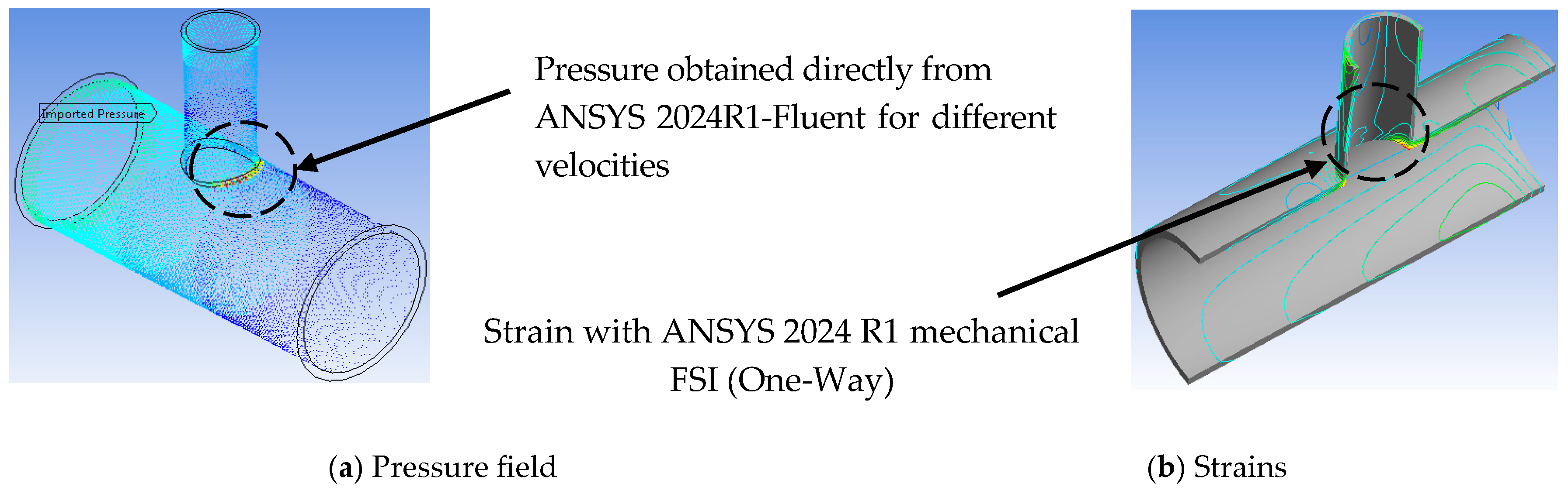
2.3. Model FSI (One-Way)

One of the most common coupled systems is the fluid–structure interaction (FSI). In this case, a dynamic phenomenon is developed. It is related to structural mechanics and fluid mechanics, and it cannot be solved independently. Due to coupling, there are forces at the interfaces of both systems [19]. In other words, the structure is deformed by the action of the flow of the fluid. It generates stresses and the structure could vibrate at its natural frequency. The velocity of the fluid is equalized at the interface. The domain of the flow is deformed at the same velocity as that of the structure. The solution to these systems (FSI) could be obtained in one-way or two-ways. The coupling is significant if the motion of a fluid flow affects a solid structure. However, the reaction of the solid in a liquid is insignificant, and vice versa [19,20].

Figure 2 shows the flow diagram of the one-way coupling analysis. The fluid flow was initially calculated until the convergence criterion was satisfied. Then, the resultant forces at the interface of the fluid and structure were estimated. The structural dynamic calculations were performed until the second convergence criterion was satisfied.

2.4. Quarter Wave Resonator

The acoustic loads were generated at the intersection of the main steam line and the safety relief valve standpipe (L) due to the interaction of the turbulent flow and the acoustic modes characteristic of this type of geometry (Figure 3).

In a closed-end tube (Figure 3), the pressure waves had a node at the open end. Under these restrictions, the boundary condition for a closed-end equals Equation (9).

$${\left[{\displaystyle \frac{{\partial P}_{man}}{\partial x}}\right]}_{closed}=0$$

(9)

The modes of vibration “n” can be calculated with the Equations (10) and (11).

$$L={\displaystyle \frac{(2n-1)}{4}}(\lambda )$$

(10)

$$f_n={\displaystyle \frac{C}{4\left(L+L_e\right)}}(2n-1)$$

(11)

where λ, is the wavelength, C is the speed of sound (it depends on the medium in which it propagates), L is the tube length, L_e = 0.425d, and n are the vibration modes (1, 2, 3, 4, 5…). Equation (11) combines theoretical models and the results of the experimental programs [21,22].

3. Materials and Methods

3.1. Experimental Method

The acoustic resonance phenomenon was obtained indirectly with the strains on a segment of the MSL of a BWR plant. It was instrumented with strain gages, as shown schematically in Figure 4. The rectangular strain gage rosettes were located at the end of such an MSL segment. The SRV was between the two points of measurement. All the information was collected with a system of acquisition data SI-VersaDAS^TM. Strain gages for high-temperature evaluations were used (HBWAH by Hitec Products, Mumbai, India). Sensor calibration and measurement uncertainty were performed based on the methodology accepted by the NRC [3,4,5,6,7,8,9,10,11,12]. They were connected under a half-bridge arrangement to minimize the effect of bending on the steam lines. In this way, the transient hoop strains were recorded [23,24]. Its transient condition was caused by the pressure fluctuating in the pipe. The frequency spectrum was obtained from the MATLAB R2023a code. Pressure was a comparison variable in this paper [24,25,26].

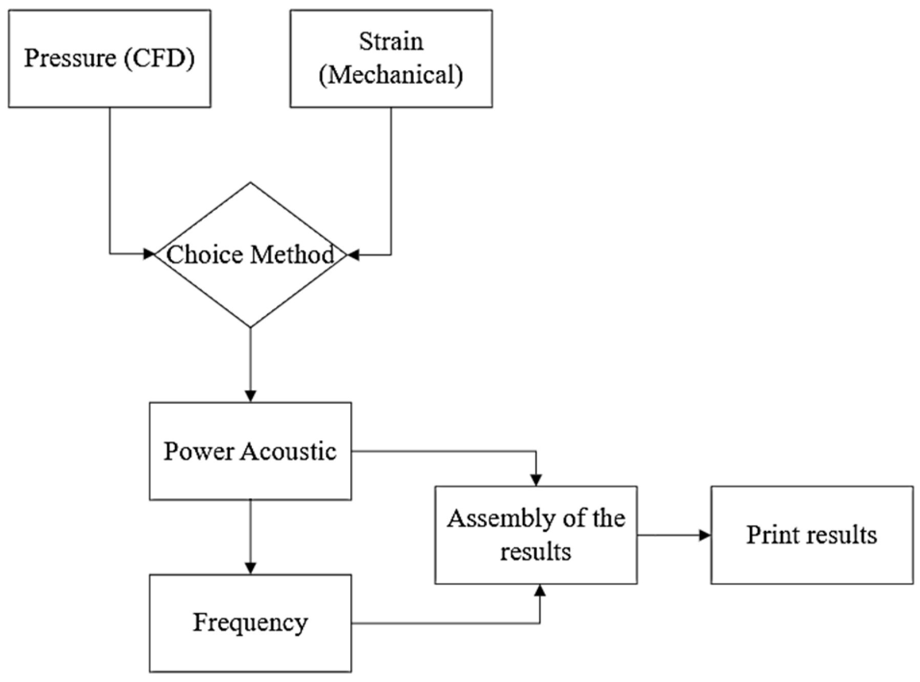
3.2. Computational Method

The acoustic analysis was conducted with the ANSYS 2024 R1 academic research program. The acoustic loads and frequencies were obtained with CFD in conjunction with the FSI one-way model and the equations of the quarter wave resonator tube, as seen in Equation (11). They were implemented using MATLAB R2023a code. The methodology followed in this research is shown in the flowchart in Figure 5.

Table 1. Geometrical dimensions of the model.

Pipe length (Lt)	88.90 mm.	Diameter branch (db)	12.10 mm.
Branch length (Lb)	138.12 mm.	Pipe thickness (et)	6.54 mm.
Diameter main pipe (dt)	28.47 mm.	Branch thickness (eb)	3.17 mm.

shows the dimensions of the geometric model used in this paper. The scale that was used was 1:8 of the original dimensions. The advantage of the proposed numerical model is its low computational cost due to the use of a steady-state numerical model. The fluctuations of the pressure, which will be transformed into acoustic noise independently, can be obtained using the strains in Equations (5) and (6) [19,26].

In the development of the 3D model, the boundary conditions for a steady-state analysis considered the velocity, turbulence, and continuity equations. Furthermore, the fluid was considered incomprehensible and under isothermal conditions. The velocity at the inlet was constant. The inlet and outlet gage pressure were set to zero. The turbulence intensity was calculated based on the hydraulic’s diameter.

The strains were obtained with a model (FSI one-way) using ANSYS 2024 R1 Mechanical. These results were compared with those obtained with the theory of thick-walled cylinders. Finally, the amplitudes and resonance frequencies were obtained with MATLAB R2023a code, using the model of the quarter-wave resonator and the numerical results of the finite element analysis. Figure 5 summarizes the methodology used in this paper. The mathematical formulation of the conditional Navier–Stokes equations of the finite volume method is shown in Equation (12), where ρ is the density, ϕ is a specific numerical property, Γ is the diffusion coefficient, S is the gross generation of the variable ϕ per unit volume, and, finally, ∇ which is the nabla operator. The Eulerian method was used because the fluid was analyzed from a fixed perspective in space. This allows for the use of simple stationary meshes that do not need to adapt to the structure deformations as it occurs in the unidirectional fluid–structure interaction.

$$\begin{gathered} {\displaystyle \frac{\partial }{\partial t}}{\int }_V^{.}\rho \varphi dV+{\oint }_A^{.}\rho \varphi dV·dA={\oint }_A^{.}{\Gamma }_{\varphi }\mathsf{\nabla }\varphi dV·dA+{\int }_V^{.}{S}_{\varphi }dV \\ \mathrm{Transient} \hspace{1em}\hspace{1em}\mathrm{Convective} \hspace{1em}\hspace{1em}\mathrm{Diffusive} \hspace{1em}\hspace{1em}\mathrm{Source} \end{gathered}$$

(12)

Figure 6 shows the flowchart of the MATLAB R2023a code. There were two methods used for the evaluation of the acoustic noise. The first one used the strains obtained in the FSI numerical simulation or the strains obtained experimentally in Equations (6), (11) and (13). The second method considered the pressures obtained by the CFD and Equations (11) and (13). The power acoustic was obtained in the lateral branch, where $P_a$ is the acoustic power (W), $I$ is the sound intensity (W/m²), $A$ is the sound propagation area in the lateral branch (m²), $P_{\mathrm{rms}}^2$ is the effective sound pressure (Pa), $\rho$ is the density of the fluid (kg/m³), $c$ is the velocity of the depropagation of sound within the fluid (m/s²) and $P_{\mathrm{ref}}$ is the reference acoustic power (watts).

$$P_a=I\cdot A\hspace{1em}\hspace{1em}I={\displaystyle \frac{P_{\mathrm{rms}}^2}{\rho c}}\hspace{1em}\hspace{1em}{L}_W=10{\mathrm{l}\mathrm{o}\mathrm{g}}_{10}\left({\displaystyle \frac{P_a}{P_{\mathrm{ref}}}}\right)$$

(13)

Regarding the boundary conditions of the CFD analysis, the model (k-e) was used with a standard wall function.

Table 2. Input flow velocities considered in the CFD analysis.

Velocity (100%)	47 m/s	Velocity (130%)	61.1 m/s
Velocity (110%)	51.7 m/s	Velocity (150%)	70.5 m/s
Velocity (120%)	56.4 m/s	Velocity (170%)	79.9 m/s

shows the velocities considered in this paper. The Strouhal number was considered based on Equation (14) [1]. S_t is defined in terms of the inner diameter branch of the stub pipe (d), the flow velocity of the main pipe (U), and the resonance frequency of the system (f_n). The steam velocity in the operation conditions of the original licensed thermal power is 47 m/s.

$$S_t=f_n{\displaystyle \frac{d}{U}}$$

(14)

In the final step, the strains were evaluated. The loading conditions (pressure) were imported directly from the CFD solution. Pressure was applied to the inner walls. They are shown in red in Figure 7. Furthermore, both ends of the pipe (blue color) were fixed.

The number of elements for mechanical analysis was 80,000 Solid-186. This is a higher-order 3-D 20-node solid element that exhibits quadratic displacement behavior (Figure 7a). The boundary conditions are shown in Figure 7b.

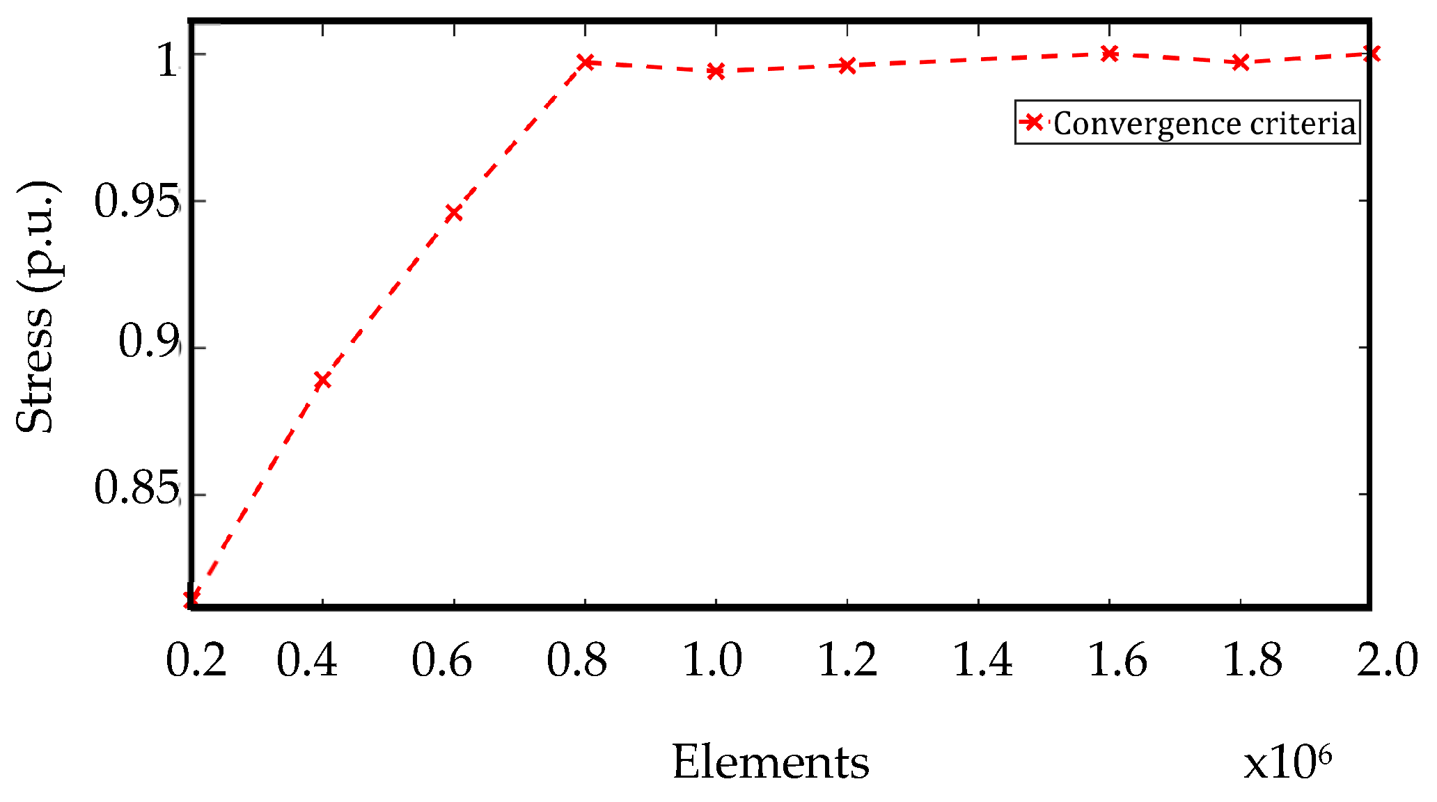
3.3. Convergence Criteria

The parameters considered in the CFD simulation were the velocity, continuity, and k-e turbulence equations. The continuity and turbulence equations converged with residuals of 1 × 10⁻³, while the convergence of the velocity equations was lower than 1 × 10⁻⁶. A convergence analysis of the mechanical evaluation was performed. The variable considered was the von Mises stress. It was normalized based on the highest stress. Figure 8 summarizes the convergence test. A mesh with 0.8 × 10⁶ elements or more is adequate.

4. Results

4.1. Estimation Experimental (Scale 1:1)

The pressure fluctuation was determined following an estimated measurement that would be made on the main steam lines of a nuclear power plant type BWR/5 (Figure 4). They are shown in Figure 9 for a controlled power uprate and stepwise of (85, 90, 95, and 100) % of the original power. The material of the MSLs is carbon steel (SA 155 KCF 70). It is equivalent to SA516 Grade 70, which is a carbon steel pipe with 0.28% carbon. Young’s modulus of a carbon pipe with 0.28% carbon at 260 °C and 315 °C is 188 MPa and 184 MPa, respectively. Therefore, Young’s modulus can be linearly interpolated as 186 MPa at 280 °C.

An estimate of the average behavior of the acoustic loads in the four branches (MSL-A, MSL-B, and MSL MSL-C-D) of a BWR/5 is shown in Figure 10. The pressure increased from 429 Pa at 85% of the original operation power to 1590 Pa. The last one is when the reactor is operated at 100% of the nominal operation.

A clean signal was obtained using the MATLAB R2023a code without considering the electrical noise (60, 120, 180, 240 Hz) and the noise caused by the jet pump (149 Hz). The acoustic loads, due to the interaction between a SRV and the MSL (Figure 11), were determined. The resonance frequency was close to 195 Hz.

4.2. Numerical Results (Scale 1:8)

The internal pressure (Figure 12a) was evaluated initially with the computational fluid dynamic code. The peak values (maximum pressure fluctuations) were located at the intersection between the closed-side branch and the main steam line (MSL). When pressure fluctuations increase due to higher fluid velocity, vortex shedding may occur due to high localized turbulence. This can cause a coupling in the acoustic modes of the pipeline and the hydrodynamic modes producing excessive vibration. It propagates through the pipeline. The structural elements are loaded dynamically, and fractures are initiated [1,2,4,10,13].

The velocity field is shown in Figure 12b. The velocity inside the branch was close to zero. Therefore, there was a significant pressure difference in the main line. This dynamic condition created a significant fluctuating condition, which generated the propagation of acoustic noise.

Six cases were studied. The first one was considered as the baseline (100%). In the other five cases, the velocity increased to 110%, 120%, 130%, 150%, and 170%. In the next step, the strains were obtained with the FSI (one-way) model. The pressure field was imported directly from the domain of computational fluid dynamics (Figure 13a) to the finite element model (Figure 13b).

Finally, the acoustic load and the resonant frequency of the first vibration’s acoustic mode were obtained with the algorithm developed in MATLAB R2023a. For this purpose, the equations of the quarter wave resonator tube were considered. Figure 14 shows the pressures calculated around the mark line (Figure 12a and Figure 13a) for the six cases considered (100, 110, 120, 130, 150, and 170%). The range of pressure was between 196 Pa to 553 Pa.

The acoustic power (Figure 15) was obtained with the MATLAB R2023acode (Figure 6), which was the result of the finite element evaluation. In normal conditions (100%), it was 97 dB. In the following cases, it increased to 114 dB for the conditions of 170%.

4.3. Comparison of the Results (Scale 1:1)

Based on the numerical results obtained previously (scale 1:8), the experimental and numerical results of the model with a scale of 1:1 were compared. The results are shown in Figure 16.

In the same way, a comparison of the frequency spectrum between the numerical and experimental results was carried out. These results are shown in Figure 17. The pressure increased at the resonant frequency. Transient effects, such as vortex shedding and coupling between hydrodynamic and acoustic modes, were not considered. However, these results are important because they allow for estimating substantial increases in fluctuating pressure and resonant frequency. Furthermore, the numerical results are consistent with those obtained experimentally.

The frequency of the first mode of acoustic resonance was 195 Hz, and the peak values were 1590 Pa and 1568 Pa for the experimental and numerical evaluation, respectively. The relative error was 1.38%. The difference between the numerical and experimental results was generated by the simplifications considered in the numerical model. The roughness of the pipe walls, steady flow, and noise contribution from other sources, among other causes, were not considered.

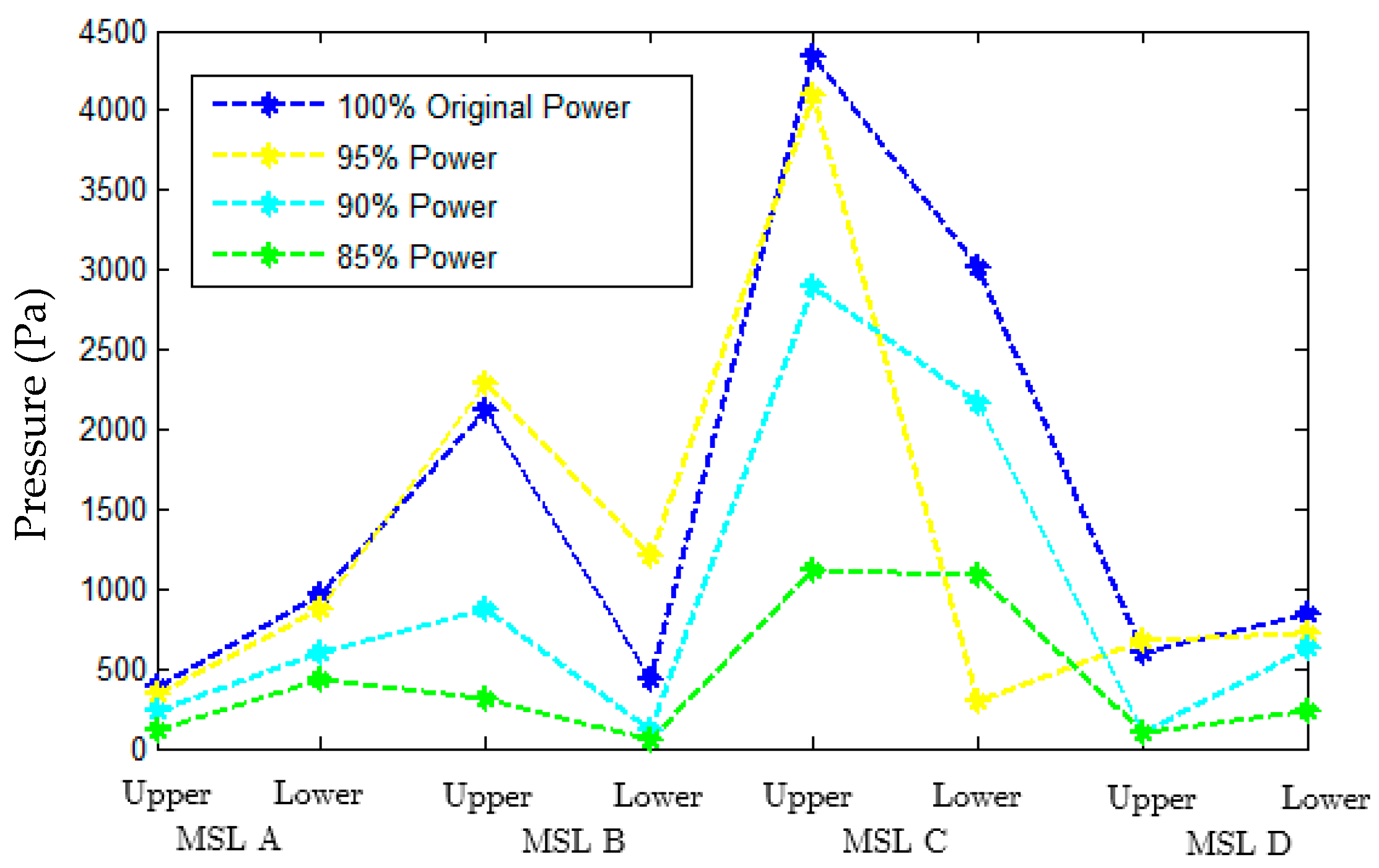
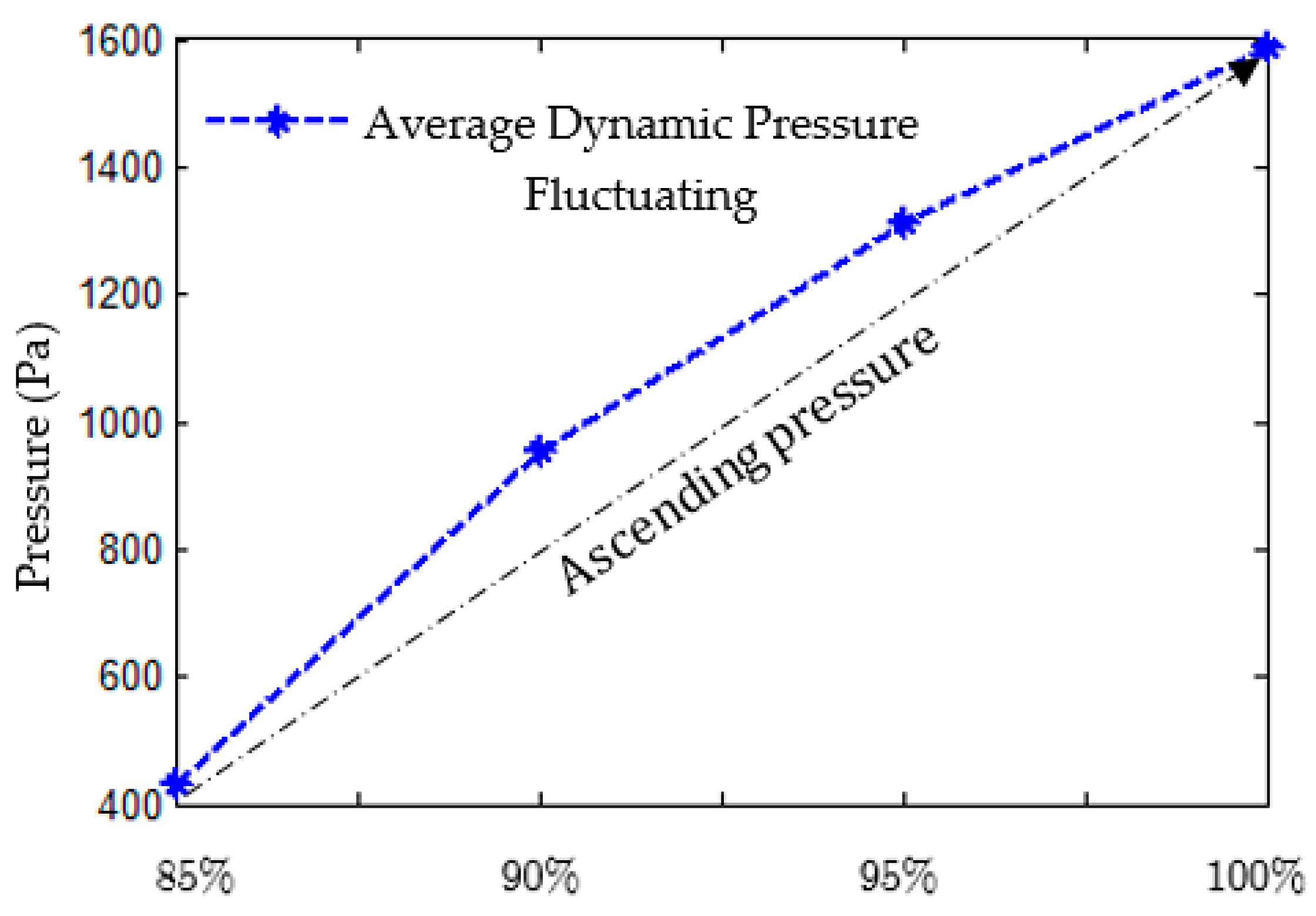
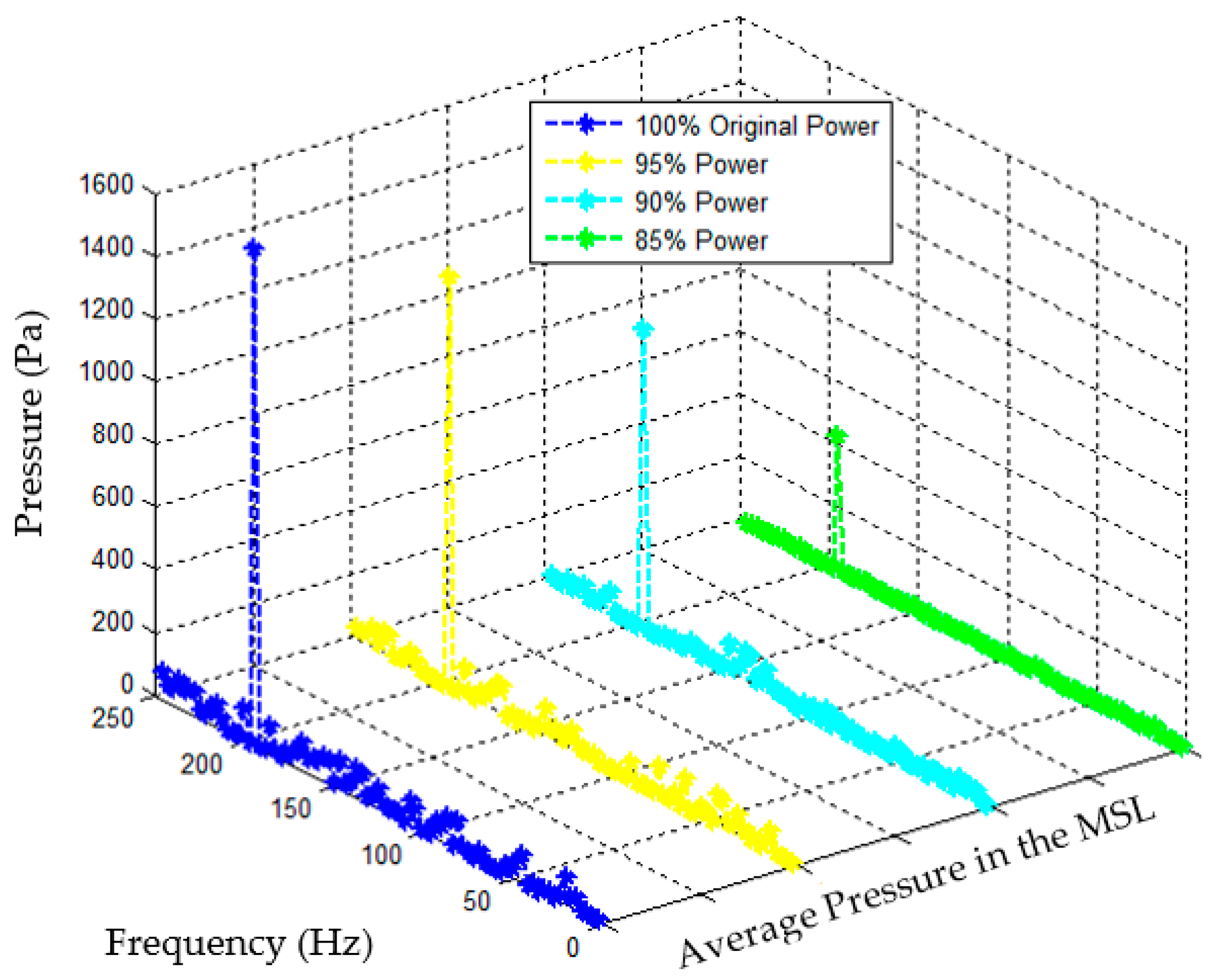
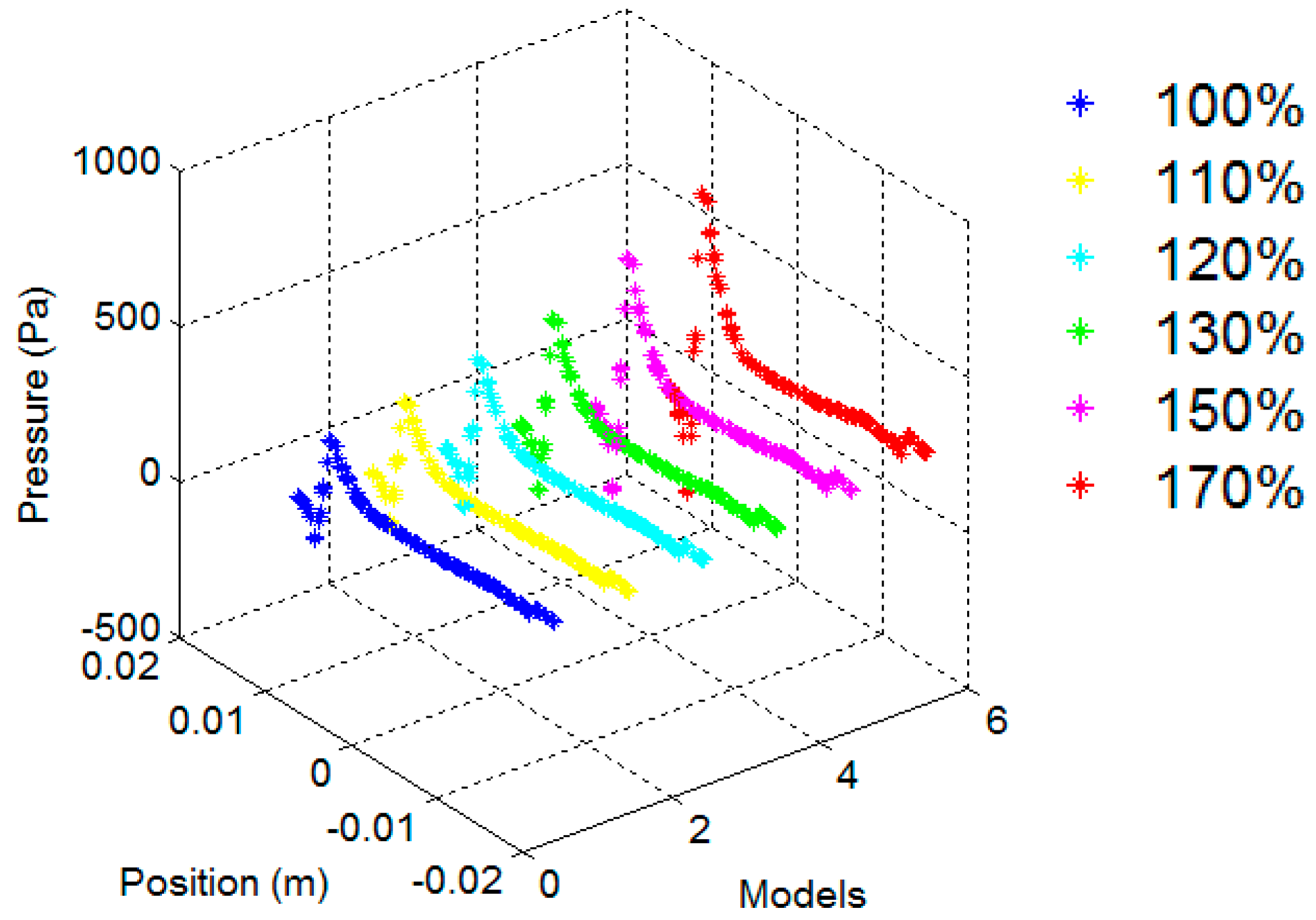
4.4. Prediction of the Power Uprate Condition (Scale 1:1)

The results obtained in the proposed methodology converge with the experimental evaluation (Figure 16 and Figure 17). Such a methodology is useful in estimating the acoustic power uprate loads and the resonant frequency. Figure 18 shows that the peak values obtained were 1570, 1890, and 2240 Pa, when the operating conditions were 100, 110 and 120%, respectively.

4.5. Prediction of the Power Uprate Condition (Scale 1:8)

The peak acoustic power calculated for the first natural frequency (1560 Hz), and for the different velocities considered, are compared in Figure 19. The acoustic power increased 4.8 times when the operating conditions increased by 120% (Figure 15). This is in line with the results presented in [6,7,8,9,10,11], where similar conditions (around 100–120%) were evaluated. The acoustic noise increased between 4 to 6 times approximately when the relation between the MSL and its branch was within a scale of 1:1 [2,6].

4.6. Discussion of the Results

The results obtained using the proposed methodology converge with the theoretical, numerical, and experimental results reported in the open literature [1,2,3,4,5,6]. This methodology is useful as an initial estimate of the acoustic loads and the resonant frequency. The different models are compared in

Table 3. Different models for the prediction of the resonant frequency.

Features and Limitations of Numerical Models	CAA Computational Aeroacoustics	Acoustic Analogy (LES and FWH)	Harmonic and Modal Analysis	Broadband Noise Modeling	FSI Coupling [This Work]
Computation cost	Too high	High	Moderate	Low	Low
Solution	Transient	Transient	Steady state	Steady state	Steady state
Accuracy	Excellent	Best	Good	Limited	Good

[6,25]. The main advantage of the proposed methodology is its low requirement for computing resources [6,18,19,25,26].

To obtain dynamic similarity, the Strouhal number was kept constant between the real model and the scale model (Table 2). This parameter ranges between 0.23 and 0.4, depending on the velocity considered in the evaluation. A low Strouhal number could indicate that the system is less susceptible to being in a resonant frequency (S_t = 0.23). On the other hand, higher Strouhal numbers would shift the analyzed system to a higher frequency. In some nuclear power plants, the acoustic resonances have been reported with the Strouhal numbers at around 0.33 (

Table 4. Strouhal numbers.

Fn1:1 (Hz)	Fn1:8 (Hz)	U (m/s)	d1:1 (m)	d1:8 (m)	St
195	1560	47.0	0.0968	0.0121	0.40
		51.7			0.36
		56.4			0.33
		61.1			0.30
		70.5			0.26
		79.9			0.23

). It corresponds to an oscillation frequency in an extended power uprate and generates significant vibrations in piping and associated components [1,2,4,5,6,10].

It is important to develop numerical models that predict the acoustic noise in the piping systems of nuclear facilities. In these cases, the computational cost can be a limiting factor. For this reason, the aim is to simplify the problem. Therefore, reliable results can be obtained before implementing a more comprehensive model that covers all the scales of turbulence and fluctuations over a wide range of frequencies. For the analysis considered in this paper, the acoustic resonance was at 1560 Hz and the acoustic power range was between 97 dB and 114 dB, when the ratio between the branch and mainline was 1:8.

When a system is in acoustic resonance, the amplitude of the acoustic waves increases considerably, generating very high-pressure peaks at specific points, as shown in Figure 11, Figure 17, and Figure 18. Damping is essential to avoid severe structural damage. Effective damping can be achieved by adding Helmholtz resonators, acoustic silencers, perforated elements, or damping chambers.

5. Conclusions

The method proposed in this paper shows a simple and quick way to obtain the magnitudes of the acoustic loads and their resonant frequencies. It can be used as a first approximation before employing transient models, such as DES, SAS, LES, or two-way fluid–structure interactions.

The methodology implemented in this paper showed that reliable results can be obtained at a low computational cost. The acoustic loads and resonance frequencies increased as these parameters approached the system’s critical velocity.

The analysis was carried out for one branch in which an SRV is located. However, the main steam line has four SRVs. For this reason, it is important to determine the contribution of the acoustic power from the other four SRVs.

The conditions of each nuclear plant are similar. However, there are small differences in geometry, temperature, pressure, and velocity. They can influence the resonance mechanism and affect the structural integrity of nuclear plants. For this reason, the Nuclear Regulatory Commission of the United States has issued a series of numerical and experimental tests implemented on scale models.

References

1. Morita, R.; Takahashi, S.; Okuyama, K.; Inada, F.; Ogawa, Y.; Yoshikawa, K. Evaluation of acoustic and flow induced vibration of the BWR main steam lines and dryer. J. Nucl. Sci. Technol. 2012, 48, 759–776. [Google Scholar] [CrossRef]
2. DeBoo, G.; Ramsden, K.; Gesior, R.; Strub, B. Identification of Quad Cities main steam line acoustic source and vibration reduction. In Proceedings of the Pressure Vessels and Piping Conference, San Antonio, TX, USA, 22–26 July 2007; Volume 4, pp. 485–491. [Google Scholar] [CrossRef]
3. Núñez, A.; Prieto, A.; Espinosa, G. Current status of steam dryer performance under power uprate in Boiling Water Reactors. Ann. Nucl. Energy 2014, 72, 447–454. [Google Scholar] [CrossRef]
4. Basavaraju, C.; Manoly, K.A.; Murphy, M.C.; Jessup, W.T. BWR Steam Dryer Issues and Lessons Learned Related to Flow-Induced Vibration. In Proceedings of the ASME Pressure Vessels and Piping Conference, Paris, France, 14–18 July 2013; Volume 3. [Google Scholar] [CrossRef]
5. Le Moigne, Y.; Andren, A.; Greis, I.; Kornfeldt, H.; Sundlof, P.; Sjunnesson, J.; Karlsson, A.K. BWR Steam Dryer for Extended Power Uprate. Nucl. Eng. Des. 2008, 238, 2106–2114. [Google Scholar] [CrossRef]
6. Ocampo, A.; Hernández, L.H.; Ruiz, P.; Moreno, N.; Urriolagoitia, G.M.; Beltrán, J.A.; Urriolagoitia, G.; Fernández, D. Simulation of the Acoustic Loads Generated in the Intersection of a Main Steam Line and its Safety Relief Valve Branch of a BWR Plant under Extended Power Uprate Conditions. Defect Diffus. Forum 2015, 362, 190–199. [Google Scholar] [CrossRef]
7. Hambric, S.A.; Ziada, S.; Morante, R.J. Overview of Boiling Water Reactor Steam Dryer Alternating Stress Assessment Procedures. ASME J. Nucl. Rad. Sci. 2018, 4, 021002. [Google Scholar] [CrossRef]
8. Tamura, A.; Okuyama, K.; Takahashi, S.; Ohtsuka, M. Development of numerical analysis method of flow-acoustic resonance in stub pipes of safety relief valves. J. Nucl. Sci. Technol. 2012, 49, 793–803. [Google Scholar] [CrossRef]
9. Au-Yang, M.K. Flow-Induced Vibration: Guidelines for Design, Diagnosis and Troubleshooting of Common Power Plant Components. ASME J. Press. Vessel. Technol. 1985, 107, 326–334. [Google Scholar] [CrossRef]
10. Hambric, S.A.; Mulcahy, T.M.; Shah, V.N.; Scarbrough, T.; Wu, C. Flow Induced Vibration Effects on Nuclear Power Plant Components Due to Main Steam Line Valve Singing. In Proceedings of the Ninth NRC/ASME Symposium on Valves, Pumps and Inservice Testing, NRC NUREG CP-0152, Washington, DC, USA, 17–19 July 2006; Volume 6. Available online: https://www.nrc.gov/docs/ml0727/ml072700042.pdf (accessed on 1 February 2023).
11. Espinosa-Paredes, G.; Prieto-Guerrero, A.; Núñez-Carrera, A.; Vázquez-Rodríguez, A.; Centeno-Pérez, J.; Espinosa-Martínez, E.-G.; Quezada-García, S.; Cázares-Ramírez, R. Signal analysis of acoustic and flow-induced vibrations of BWR main steam line. Nucl. Eng. Des. 2016, 301, 189–203. [Google Scholar] [CrossRef]
12. U.S. Nuclear Regulatory Commission. Comprehensive Vibration Assessment Program for Reactor Internals during Preoperational and Initial Startup Testing 3, Regulatory Guide 1.20, Rev.4. 2017. Available online: https://www.nrc.gov/docs/ML1605/ML16056A338.pdf (accessed on 1 February 2023).
13. NRC. 2002. Failure of Steam Dryer Cover Plate After a Recent Power Uprate. U.S. Nuclear Regulatory Commission. Washington, DC, NRC Information Notice 2002-26. Available online: https://www.nrc.gov/docs/ML0225/ML022530291.pdf (accessed on 1 February 2023).
14. NRC. 2013. Programs for Monitoring Boiling-Water Reactor Steam Dryer Integrity. U.S. Nuclear Regulatory Commission, Washington, DC, NRC Information Notice 2013-10, ADAMS Accession No. ML13003A049. Available online: https://www.nrc.gov/docs/ML1300/ML13003A049.pdf (accessed on 1 February 2023).
15. Brazhenko, V.; Cai, J.-C.; Fang, Y. Utilizing a Transparent Model of a Semi-Direct Acting Water Solenoid Valve to Visualize Diaphragm Displacement and Apply Resulting Data for CFD Analysis. Water 2024, 16, 3385. [Google Scholar] [CrossRef]
16. Jones, W.P.; Launder, B.E. The Prediction of Laminarization with a Two-Equation Model of Turbulence. J. Heat Mass Transf. 1972, 15, 301–308. [Google Scholar] [CrossRef]
17. Blazek, J. Turbulence Modelling. In Computational Fluid Dynamics: Principles and Applications; Elsevier: Amsterdam, The Netherlands, 2005; Volume 7, pp. 227–270. [Google Scholar] [CrossRef]
18. ANSYS Fluent User’s Guide, Chapter 15. 2024. Modelling Turbulence, R2, 2061-2161. Available online: https://ansyshelp.ansys.com (accessed on 1 March 2024).
19. Benra, F.K.; Dohmen, H.J.; Pei, J.; Schuster, S.; Wan, B. A comparison of one-way and two-way coupling methods for numerical analysis of fluid structure interactions. J. Appl. Math. 2011, 2011, 853560. [Google Scholar] [CrossRef]
20. Chen, S.S. Guidelines for the Instability Flow Velocity of Tube Arrays in Cross-flow. J. Press. Sound Vib. 1984, 93, 439–455. [Google Scholar] [CrossRef]
21. Ziada, S.; Shine, S. Strouhal Numbers of Flow-Excited Acoustic Resonance of Closed Side Branches. J. Fluids Struct. 1999, 13, 127–142. [Google Scholar] [CrossRef]
22. Ziada, S.; Lafon, P. Flow-Excited Acoustic Resonance Excitation Mechanism, Design Guidelines, and Counter Measures. Appl. Mech. 2014, 66, 010802. [Google Scholar] [CrossRef]
23. Szasz, G.; Fujikawa, K.K.; Ananth, R. Dynamic Pressure Data Acquisition Via Strain Gage Measurements. In Proceedings of the ASME International Design Engineering Technical Conferences and Computers and Information in Engineering Conference, Long Beach, CA, USA, 24–28 September 2005; Volume 1, pp. 1263–1269. [Google Scholar] [CrossRef]
24. Szasz, G.; Fujikawa, K.K.; DeBoo, G. Assessment of Steam Line Dynamic Pressures Using External Strain Gage Measurement. In Proceedings of the ASME 2006 Pressure Vessels and Piping/ICPVT-11, Vancouver, BC, Canada, 23–27 July 2006; Volume 3, pp. 761–765. [Google Scholar] [CrossRef]
25. Coloniusa, T.; Lele, S.K. Computational aeroacoustics: Progress on nonlinear problems of sound generation. Prog. Aerosp. Sci. 2004, 40, 345–416. [Google Scholar] [CrossRef]
26. ANSYS Fluent User’s Guide, Chapter 23.2024. Predicting Aerodynamically Generated Noise, R2, 2659–2701. Available online: https://ansyshelp.ansys.com (accessed on 1 March 2024).
Figure 1. Stresses generated on the cylinder wall (t).
Applsci 15 03974 g001
Figure 2. Flow diagram of the one-way solution.
Applsci 15 03974 g002
Figure 3. Fundamental frequency f0 of a semi-closed tube.
Applsci 15 03974 g003
Figure 4. Instrumentation on the main steam line.
Applsci 15 03974 g004
Figure 5. Flowchart of the methodology.
Applsci 15 03974 g005
Figure 6. Flowchart of the MATLAB R2023acode.
Applsci 15 03974 g006
Figure 7. Mesh and boundary conditions.
Applsci 15 03974 g007
Figure 8. Mesh independence.
Applsci 15 03974 g008
Figure 9. Pressure measurements of the MSLs.
Applsci 15 03974 g009
Figure 10. Pressure average measurements of the interior of the MSL.
Applsci 15 03974 g010
Figure 11. Pressure average measurement over the interior surface of the MSL.
Applsci 15 03974 g011
Figure 12. Pressure and velocity fields obtained with a CFD code.
Applsci 15 03974 g012
Figure 13. Numerical imported pressure directly from the CFD.
Applsci 15 03974 g013
Figure 14. Pressure evaluated around the stress concentration point.
Applsci 15 03974 g014
Figure 15. Numerical acoustic load generated with the MATLAB R2023a code.
Applsci 15 03974 g015
Figure 16. The prediction and comparison of the results for an output power of 100% (scale 1:1).
Applsci 15 03974 g016
Figure 17. Comparison of the acoustic load for power output at 100% of the conditions of operation.
Applsci 15 03974 g017
Figure 18. Numerical prediction of the power uprate condition.
Applsci 15 03974 g018
Figure 19. Numerical acoustic power evaluated with a scale of 1:8.
Applsci 15 03974 g019