Abstract
Arid and semi-arid environments are characterized by highly variable and unpredictable rainfall patterns, which significantly affect the structure and function of natural ecosystems. Understanding the interconnected relationship between climate variability, forage availability, and livestock dynamics in these regions is crucial to ensure sustainable management. This study provides novel insights into the effects of rainfall variability on natural forage resources and livestock populations in Botswana. In this arid region, traditional livestock farming remains a key economic and food security pillar. By employing a mathematical model based on plant–herbivore interactions, this article quantitatively evaluates the impact of changes in rainfall timing and intensity on forage biomass and, subsequently, livestock populations. A robust analysis of critical threshold values for ecosystem sustainability is possible when real-world climate data are incorporated. This study examines the effects of harvesting and rainfall variability on livestock dynamics across different locations in Botswana. Delayed rainfall leads to a sharp decline in livestock, while Sehitlwa sees biomass loss without a notable reduction in herd size. In Kgagodi, for example, livestock numbers decline by 37% without harvesting, but they remain stable with controlled harvesting. Conversely, Letlhakeng experiences a 6% increase in livestock numbers despite delayed rainfall, which results in a biomass decline. Both Mabutsane and Letlhakeng maintain stable livestock numbers. The findings confirm that early and intense rainfall enhances livestock productivity, while delayed or reduced rainfall leads to population decline, aligning with observed trends in historical data. Additionally, the study underscores the potential of adaptive livestock harvesting strategies as a viable approach to mitigating climate-related risks in grazing systems. As this work integrates theoretical modeling with empirical climate data, it contributes to understanding arid land dynamics, providing a predictive method for assessing ecosystem responses to climate variability. These insights are invaluable for policymakers, conservationists, and local farmers seeking sustainable livestock management practices in the face of changing climatic conditions.
1. Introduction
Livestock, which refers to domesticated animals raised for various purposes, is a global resource for both developing and industrialized societies [1,2,3]. They provide multiple benefits that include food, clothing, fuel, nutrient cycling for soils, income, and employment [4,5]. Due to their great benefit, they become the largest users of land and biomass globally [6]. They occupy one-third of the global ice-free terrestrial land surface [6]. This is because producing feed crops and grazing pastures for livestock requires substantial amounts of land. On the other hand, the demand for agricultural products (plant and livestock-based) is expected to increase with the expected increase of the world population to 9.7 billion in 2050 and 10.9 billion in 2100 [7]. In other words, in the 21st century, agriculture will have to scale up to feed a human population that is expected to increase by 30% in 2050 [7]. However, this cannot happen at the expense of animal welfare, an increase in the environmental footprint, or even at a higher cost, which would limit market access for developing countries. Therefore, it is imperative to optimize the whole food chain to overcome these challenges.
In arid and semi-arid regions like Botswana, livestock production is central to rural livelihoods [8], with cattle, goats, and sheep serving as the primary sources of income and food security. The productivity of these livestock populations is deeply tied to the availability of natural forage [9], such as grasses and shrubs, which in turn are directly influenced by rainfall patterns [10,11]. In Botswana, where rainfall is highly variable [12], both in timing and intensity, even slight deviations in rainfall patterns can lead to periods of forage scarcity, negatively affecting livestock health, reproduction, and overall population dynamics [11,12]. Traditional farmers in Botswana, who rely heavily on rainfall as an indicator of forage availability, are particularly vulnerable to these changes.
Unlike modern scientific methods that incorporate factors such as soil moisture to predict forage growth and livestock harvest [13], traditional livestock farmers [14] base their decision-making primarily on their understanding of rainfall patterns and duration [8,15]. While valuable for its historical and practical basis, this reliance on rainfall observation may leave these communities less equipped to handle the growing uncertainties brought about by climate variability. As rainfall becomes increasingly unpredictable due to climate change [16,17], there is a pressing need to understand better how these changes impact natural forage availability so that traditional farmers can enhance their livestock management practices.
Changes in rainfall intensity and timing have a direct impact on the availability of forage, which subsequently influences livestock productivity and the long-term sustainability of rangelands. Understanding these interactions is crucial for developing adaptive management strategies that improve livestock resilience amid changing climatic conditions. Several studies have examined the relationship between rainfall and forage production [17,18,19,20]. For example, Giridhar et al. [21] found that, in the coming decades, crops and forage plants will be increasingly affected by rising temperatures, elevated carbon dioxide, and wildly fluctuating water availability due to changing precipitation patterns. Similarly, Cain et al. [22] reported that forage conditions (quantity and quality) in arid and semi-arid regions are influenced by unpredictable spatial and temporal patterns in rainfall.
Research further illustrates how fluctuations in rainfall directly affect livestock productivity [10,11,19,21,23,24]. For example, Baumgard et al. [23] indicated that years of low rainfall correlate with decreased weight gain of livestock and higher mortality rates. In contrast, Kgosikoma and Batisani [10] and Kassa et al. [17] emphasize that practices such as supplementation, mobility, and harvesting, respectively, can mitigate these effects by optimizing forage use during both wet and dry seasons.
Previous studies also examined the relationship between soil moisture and forage availability in Botswana [13,17]. However, this approach may not fully align with the practices and realities of traditional livestock farmers. These farmers primarily rely on their intuition and historical knowledge of rainfall patterns and duration to manage their livestock rather than scientific indicators such as soil moisture levels. Additionally, traditional farmers in Botswana often lack access to advanced climate data or technologies [17], and their management decisions are based more on observations of rainfall than on an understanding of how water infiltrates and is stored in the soil.
While some of the studies reviewed link rainfall to forage biomass and livestock productivity, they often lack an integrated quantitative approach that considers both the intensity and timing of rainfall events in shaping forage production and livestock dynamics. The existing mathematical models for plant–animal interaction have limitations, as they fail to capture the effect of rainfall variability (both in the timing and intensity) on livestock production. However, this issue can significantly impact agricultural planning and the livelihood of traditional farmers, more especially in arid and semi-arid environments. This study employs a mathematical model to assess how variations in rainfall influence natural forage availability and livestock populations over time. By incorporating spatial and temporal rainfall variability, the model provides insights into optimal grazing and livestock management strategies for climate adaptation.
This manuscript is structured into four sections, not counting the references. In Section 2, we briefly describe the materials and methods: the study area and the formulation and analysis of the mathematical model. Section 3 presents the findings derived from numerical simulations, followed by an in-depth discussion of these results. The manuscript concludes with a set of recommendations outlined in Section 4.
2. Materials and Methods
2.1. Study Area
Botswana (18–27° S; 20–29° E) is a large semi-arid country with a small population of about 2,379,000 [25], and it covers an area of approximately 581,730 square kilometers [26]. Botswana is landlocked by Namibia to the west and north (the Caprivi Strip), Zambia and Zimbabwe to the north–west, and South Africa to the south–east and south.
According to the Center for Applied Research of Botswana [27], the country has a mean altitude of 3300 feet (1000 m) and is primarily comprised of a sand-filled basin with gently undulating plains that rise to highlands in neighboring countries. The highest point is 4888 feet (1490 m) in the hills north of Lobatse in southeastern Botswana, while the lowest point is 2170 feet (660 m) at the country’s easternmost point in the Limpopo Valley. Rainfall in the country is generally low, ranging from 250 mm per annum in the southwest to an annual mean of 650 mm in the northern regions.
The country is divided into four main environmental regions, as shown in Figure 1. The hardveld region features rocky hill ranges and areas with shallow sand cover in eastern Botswana. The sandveld region consists of deep Kalahari sand found in the western part of the country. Additionally, there are the Mopane savanna and wetlands regions.
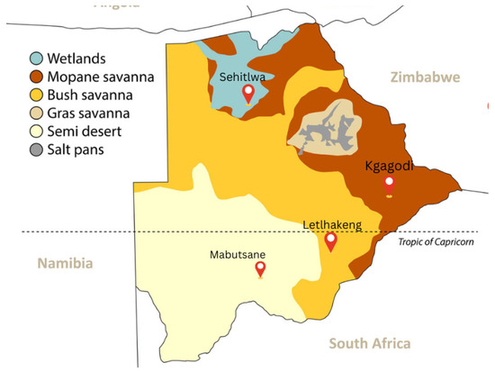
Figure 1.
Sites location on a map of Botswana with different environmental vegetation taken from [26].
Most of the agricultural production in Botswana is from livestock agriculture [28], with traditional livestock-keeping activities dominating commercial production, covering approximately 60 percent of the country’s land [29]. However, this traditional animal production system is based on a rain-fed agricultural setting, which faces significant challenges due to a lack of moisture.
For our study, we selected four locations: Mabutsane, Sehitlwa, Letlhakeng, and Kgagodi, each situated in distinct vegetative regions, as shown in Figure 1. These areas represent different soil types and different types of vegetation. Mabutsane represents the semi-desert region (sandveld), Kgagodi exemplifies the Mopane savanna area (hardveld), Letlhakeng lies in a transitional zone between hardveld and sandveld, and Sehitlwa is characterized as a swamp or wetland area.
2.2. Model Formulation and Description
To formulate a mathematical model for the interaction between plants and livestock in the given spatial area, we used the classical predator–prey structure as a base model with logistic growth dynamics for plant biomass. By employing the process-based modeling approach, the plant growth rate is assumed to depend on the seasonal effects of the environment as well as the actual precipitation.
In this section, we proceed to the construction of a mathematical model for the plant–livestock interaction dynamics in order to estimate the potential livestock production in Botswana supported by natural forage in climate variation. The basic mathematical system we consider is the classical Lotka–Volterra type model in the version presented by Asfaw et al. [9,16,30]. We assume that the following hypothesis holds for our model.
- Livestock depend on the availability of food to reproduce. Their nutrients are mostly found on natural forage if they are not given supplementary feeds [31].
- There is a relationship between seasonal variation of rainfall and plant growth. There is a significant season-to-season variability in rainfall amount and distribution [32]. Within the semi-arid forests, there may be little seasonal rhythm in the growth and development of vegetation as a whole. Summer, spring, and autumn are seasons experiencing rainfall; particularly, the summer season is known for extreme rainfall and is well distributed in most parts of the country [12]. A season varies from three to four months. More vegetative growth starts around spring, and flourishing occurs mid-spring up to autumn. In winter, there is no vegetation growth because of no rainfall and extreme cold temperature variation.
Assume that the state variables for the model system are given by the plant biomass represented by P and the livestock density represented by L. Then, using the above assumptions, the dynamics of the system at any time can be written as:
where the values , and d are positive constants, with K representing the environmental carrying capacity for plant biomass, c is the conversion rate of the consumed plant into livestock, is the off-take rate, and d is the mean natural death rate for livestock. We take these parameters as constant because the effect of rainfall in them is very insignificant to the level that it can be ignored. is the rainfall-dependent plant growth rate, and is the functional response of consumption of plants by livestock through grazing and browsing.
Now we give descriptions of important parameters used in the model and their assumptions.
- A constant per-capita death rate of livestock (d):, It is assumed in this study that the mean death rate of livestock is constant as used in [33]. However, some authors [9,16] consider a non-constant or plant-dependent death rate with the assumption that livestock die off exponentially in the absence of plants. If livestock eat more, they will be less likely to die from starvation or from the consequences of weakness brought by hunger.
- Harvest rate, : This is considered a constant, and it represents the human interference in the system by removing livestock from the system at a constant rate. It is the removal of animals through consumption and/or selling.
- Functional response function, : This is the intake rate of the livestock as a function of plant biomass. It is also associated with the reproduction rate of livestock as a function of plant biomass. In this work, we consider the Holling type II function, , as described in [9,16].
- Plant growth rate function, : The amount and distribution of rainfall have a strong impact on the development of plants. A certain minimal amount of moisture is needed to activate seed germination and reproduction. That is, they become abundantly green and grow during the rainy season, and they die out or do not grow during droughts. The rate or amount in which rain is received at a time could be too much or too low for the environment. Too much water injures plants, compacts soils, and leads to soil erosion [34]. Root loss occurs when excess water reduces oxygen in the soil. Extreme summer rain can leach nitrogen out of the soil. Excessive rainfall is not necessarily useful or desirable at all times. Some of it is unavoidably wasted, while some may cause destruction [34]. If the average rainfall is much lower than the ‘ideal’ amount needed, it could lead to the dying of plants and grasses [35]. Most grasses in Botswana are seasonal; that is, they grow in summer during the rainy season and become dry and die out during the winter season when rainfall reduces or is not at all.Therefore, in this paper, we consider rainfall to be a factor that affects plant growth rate. The plant growth in this study refers to the increase in plant biomass that is edible by the livestock, and we represent this information by the model below for :where A is a given constant, and is the value that takes the effects of soil type and soil texture on the growth rate. represents daily rainfall data, is the mean of rainfall data, represents the standard deviation from while . We also assume that is -periodic, with days (or 1 year).
- Sinusoidal response term: The term represents the rate of plant growth at the beginning of the spring season. Plants are structurally smart and can sense their environments changing, and those changes signal them to start to grow again. For example, when plants experience a number of warm days, they are prompted to start growing again. Buds begin to appear on trees. Glucose that was produced during photosynthesis and stored in the roots will provide plants with energy and food for budding. The delay of rain will make plants finish stored glucose and begin to die [36].
- Soil structure, : This term represents the physical characteristics of soil in reducing the growth of plants. According to Passioura [37], roots grow most rapidly in very friable soil, but their uptake of water and nutrients may be limited by inadequate contact with the solid and liquid phases of the soil.
With the above modifications, the model system that we study, therefore, takes the following form:
where the plant growth rate function (3) is included in the system to obtain a non-autonomous ordinary differential equations.
2.3. Mathematical Analysis
It is biologically relevant to assume that all parameters in Model system (4) are positive since they represent rates. Regarding the growth rate function , we assume that in is a positively -periodic continuous function. This assumption is a natural way to introduce seasonality in these types of models. Given a continuous -periodic function . We use notation and for maximum and minimum rainfall, respectively, represented by
That is, our -periodic function cannot be negative, and the maximum cannot be infinity. According to Botswana Environmental statistics [25], the maximum amount of rainfall in Botswana is around 650 mm per year. Therefore, we bound the rainfall amount so that it will not exceed the maximum amount. We assume that the parameters A and satisfy .
2.3.1. Well-Posedness of Model
Model (4) is a nonlinear system of non-autonomous differential equations. We rely on the numerical methods to obtain a solution. We want to determine whether the solution remains bounded for all values of t. Boundedness means the value of does not become infinitely large or negative as t varies.
Equation (3) is a linear first-order non-autonomous differential equation, which can be written as
where and , with initial conditions , .
If we solve (5) using an integration factor, then our unique solution becomes
Since and , the integral in (6) implies
Then we obtain
Thus, we have the following two lemmas.
Lemma 1.
Equation (5) is a linear dynamical system in the following compact interval, which exhibits an attractive nature
Lemma 2.
Equation (3) admits a unique non-negative ω-periodic solution , which is globally attractive in and is given by
Once Equation (3) is separately solved, as explained above, we incorporate its solution where appropriate in the remaining equations of the model (4). Since is globally attractive in , the system (4) is asymptotically equivalent to the following non-autonomous differential equation system:
such that and . For all state variables and , we should ensure that for all positive times, these state variables must be non-negative for each solution of the system starting with and . This is equivalent to saying that the positive quadrant is positively invariant. We denote by the non-negative quadrant and by the positive quadrant.
Lemma 3.
(Positivity). All solutions of system (9), starting in , remain positive.
Proof.
From the first equation of system (9), we obtain
From the second equation of the system (4), and using (10), we obtain
If then and . That is, if there is no plant, the livestock population will be extinct. If , then for all , and then the plant population obeys the logistic growth rate law for . Clearly, exponential functions are always positive. Therefore, if and , we have the whole dynamics ranging within the first quadrant, that is, and . This is obvious from the system (4) using the Cauchy–Lipschitz theorem (can be found in Theorem 2.2 in [38] or Theorem 2.1 in [39]), as the P- and the L- are orbits; the positive quadrant is positively invariant. □
We can also verify the outcomes of Lemma 3 through numerical techniques. Figure 2 illustrates the phase portrait diagram of model system (9) using the parameter values listed in Table 1, along with initial population values of and .
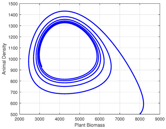
Figure 2.
Phase portrait of model system (9).

Table 1.
Initial values of the variables and parameter values used for simulations.
The depicted graph in Figure 2 reveals a stable limit cycle within the system. It indicates that regardless of the initial point within the trapping region, the system ultimately converges to a solution on this orbit and is always positive.
2.3.2. Boundedness
Lemma 4.
For model system (4), let with . Let . Then, for any positive , we have and .
Proof.
The proof of Lemma 4 closely resembles that of Lemma 2.2 in [9], where a similar argument is presented. Notably, modifications to the growth rate function do not alter the essence of the proof. □
Theorem 1.
The set on which the system (4) is defined, is positively invariant, where and
Proof.
From the first equation of the model system (4), it is clear that if then . Moreover, from the second equation when and , we have . Therefore, we can conclude that the trajectory of the solution of the system is directed inward on the boundary points of the positive quadrant, that is, on the set . Hence, the conclusion of the theorem follows immediately from Lemma 1 and 3 above. □
The above permanence of the system verifies that, for the model system (4), with the given non-negative initial conditions, there exists a -periodic solution to it that remains in the domain for all , and the solution is globally attractive. Thus, the system is mathematically and biologically well posed.
2.3.3. Coexistence Solution and Livestock-Free Solution
When the livestock population is always positive, that is, , from Equation (4) the term
represents the average rate of emergence of livestock and is an increasing function of P. Similarly, the term represents the rate of removal of livestock. If , then the rate of livestock mortality will always be higher than its emergence. Hence, the livestock population eventually will decay to extinction. Therefore, for the non-extinction of livestock, we must always have a condition that
Thus, define to be a threshold function value for the system.
Since is periodic, the solution of (4) also becomes periodic and continuous, and there exist and such that , where and are solutions of Equation (9) corresponding to and , which are constant values. Therefore, the livestock emergence rates in each case are related as . On the other hand, Equation (12) becomes
using the solution of (9), and we can find a critical threshold value that ensures the stability of coexistence. Considering the provided estimates, our focus will be on examining both the upper and lower bounds of . We start with the upper system which, using the fact that, for all , . Then, the upper bound reproduction ratio is obtained as follows:
Our next step is to determine the lower bound for the threshold, which is obtained by using the fact that, for all , . Then, we define
It should be noted that the interesting qualitative results obtained in this section are due to the estimates of the complex threshold value. In this regard, the time-average basic reproduction number, , of the non-autonomous system (9) can be obtained by setting the time-dependent -periodic function to its time average within the period , as
In doing this, we have
Hence, we have the following theorem.
Theorem 2.
The livestock basic reproduction number of system (4) is bounded from below by and from above by . That is .
The reproduction ratio in Theorem 2 can be illustrated graphically, showing that each of our four site areas exhibits distinct basic reproduction ratio values due to variations in rainfall across these locations (Figure 3). The analysis of livestock population growth rates as described by the threshold value, , in these four site areas from 2020 to 2023 reveals a concerning downward trend (Figure 3), with critical periods observed around day 250 and day 650, which correspond to September 2020 and September 2021, respectively. During these times, values approached 1, indicating a heightened risk of livestock population decline that is potentially linked to seasonal rainfall patterns [40]. This observation aligns with findings by Puoetsile et al. [41], who documented similar declines in livestock data trends in the region. Forecasts made using Neural Network Autoregression (NNAR) models, as presented by Puoetsile et al. [41], and supported by historical data [42], confirmed the persistence of this decline. The uniformity of this trend across all studied areas highlights an urgent need for further investigation into contributing factors, such as forage availability and environmental stressors, to develop adaptive strategies for sustaining livestock populations.
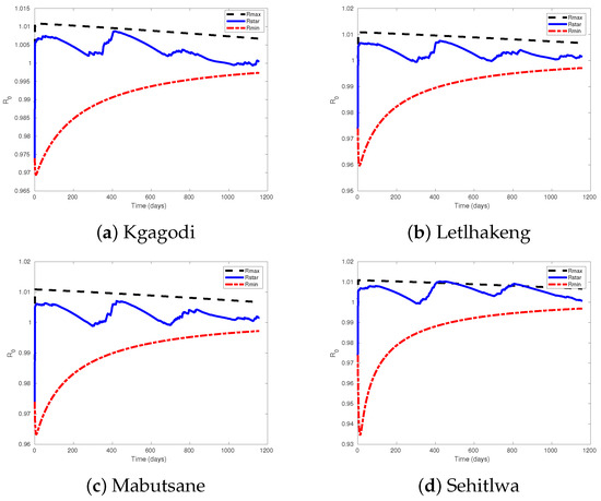
Figure 3.
Figure showing the lower bound and upper bound of reproduction ratio with the value of averaged reproduction ratio.
Theorem 3.
Suppose the model system (4) is given with a positive initial plant population . If , then as time goes on, the livestock population decays to zero, whereas the plant population grows to the carrying capacity K of the environment.
Proof.
Let us bound the values of from above. To do this, we bound the livestock birth rate from above. Since the maximum livestock emergence rate is , to bound this from above for , we have bounded above by a function , which when has the property that as Hence, for any such that for . Using Lemma 3, we have the relation
Moreover, from Lemma 3 and [43], we have for , implying that for all . Then, we can observe that
Hence, for , we may choose small enough such that is a negative constant, say (where ). Then, we have for where for , and is a solution of . Since L satisfies positivity and is bounded above, then is a non-negative and finite. Hence as , which implies that as , since for .
Finally, we shall show that as . We choose any Then there exists such that for . Now, choose such that ; since as , there exists such that for . Using this and also positivity, we have , for . Then from (9), we have . We also know that is bounded and positive. Then for where and is a solution for . Since by definition , then , so that by solving explicitly for we have which solves to for some constant . Now, as , since , we have or
In particular, for for some . But by our choice for , we have . So that . Hence for . Combining our observations and letting , we see that for . Thus as , as required. □
Theorem 3 states that when the birth rate of livestock is lower than the mortality rate, the number of livestock dying surpasses the number of newborns. Consequently, in the long term, this circumstance leads to the growth of the plant population up to the maximum capacity of the environment, while the livestock population eventually faces extinction.
The threshold condition establishes a relationship between the parameters of the model system and the minimum and maximum values achievable by the variables within the varying quantities. Simply put, it delineates the range of resources available and subsequently determines the minimum and maximum number of possible livestock that the system can sustain, facilitating the coexistence of both the plant and livestock populations without risking extinction. To uphold this equilibrium, we have the option to either introduce more livestock or reduce their numbers (via harvesting) within the system.
Note that , so that . The threshold value, , helps us to specify the non-extinction condition for the livestock population and hence can be considered as the effective reproduction number of the livestock population. That means to guarantee coexistence of both populations, we need this ratio to be always greater than unity, that is, .
Theorem 4.
Suppose that . For , , if where is a positive constant then as .
Proof.
Suppose . Then, since , let us define as a very small positive number, to be a sufficiently large number such that , and also let .
Then, . Let us choose so that . When using the equation for and Lemma 3, we have
which implies that
Now for , and because of the choice of , we have ; using our choice of , we obtain
Hence,
Moreover, using the equation for and Lemma 3 since , and , , we have
Then, using Equation (19) we obtain
But then for . Hence, . Again from the definition of , we can clearly see that
Hence This implies that the livestock population will not go to extinction, that is, for □
Theorem 4 tells us that coexistence is possible in our system, but it does not tell us what happens to the size of the population as time goes on. The answer to this is found in Theorem 3.3 from [9]. This can also be represented by simulation, as shown in Figure 4. This figure delineates the range of resources (forage) available and subsequently determines the minimum and maximum number of livestock that the system can sustain, facilitating the coexistence of both the plant and livestock populations without risking extinction. This is referred to as a stable limit cycle. To uphold this equilibrium, we have the option to either introduce more livestock or reduce their numbers (via harvesting) within the system.
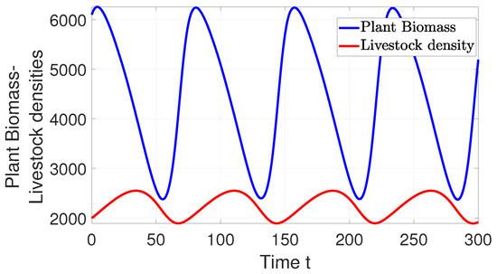
Figure 4.
Figure showing stable limit cycle of both plants and livestock population when parameter values remain constant.
3. Numerical Simulations and Discussion
3.1. Parameter Values
In this section, we presented parameter values used for simulations, time series of the model dynamics simulations for plant and livestock populations, sensitivity analysis, and simulations for the spatial distribution of possible plant and livestock production.
The plant’s growth rate, , is determined by multiple factors, including the quantity of rainfall and soil properties such as texture, structure, and type. Rainfall data, denoted as , exhibits -periodicity, and the time series data were retrieved from satellite observations. It’s essential to note that the estimation is derived from a single point assumed to be representative of the entire grid cell within a given region.
Despite various scientific methods used for soil classification [44,45], scientists commonly employ terms such as sandy, clay, and loam to characterize soil, primarily focusing on its texture. Soil texture is determined by the sizes of mineral particles it contains. The proportion of these particle sizes influences the volume of pore space within the soil, affecting its capacity to retain air and water. Finer soil particles tend to compact more when moist, resulting in the stickiness often associated with clay soils. On the contrary, sandy soils, composed of larger particles, tend to drain water rapidly, hindering healthy plant growth and typically containing fewer nutrients. However, they are easier to cultivate. To address these distinctions, we aim to select a value for the variable that approximates nearly 0 for clay soils while approaching 1 for loam soils.
The assumptions we took for the rest of the parameters are summarized in Table 1.
3.1.1. Effects of Change in Rainfall Intensity in Botswana
This study examines the effects of rainfall patterns in Botswana, with a focus on four distinct types of vegetation cover, shown in (Figure 1). Our analysis involves varying the intensity of rainfall data collected from 2008 to 2023.
It should be noted that an increase in the intensity of rainfall generally benefits both plant and livestock populations in a plant–livestock ecosystem. For plants, the additional rainwater availability enhances growth in biomass production and reproductive success, leading to a higher plant population density. This abundance of plant resources, in turn, provides livestock with more food, improving their survival rates, health, and reproductive success. An increase in rainfall intensity also makes water available for livestock to drink. Consequently, the livestock population is likely to increase in number due to the ample food supply and water available. In such a case, farmers are able to have more harvest from their animals. In contrast, a reduction in rainfall intensity results in detrimental effects on the ecosystem. Decreased rainfall diminishes soil moisture and groundwater, leading to stunted plant growth and forage scarcity. These conditions can significantly impair livestock populations by limiting both their food and drinking water availability, ultimately compromising their health and reproductive potential. Through this investigation, we aim to contribute to a comprehensive understanding of how fluctuations in rainfall patterns impact the intricate balance of the plant–livestock ecosystem in Botswana.
Figure 5 reveals a clear relationship between rainfall intensity, livestock population, and plant biomass. When rainfall intensity is decreased on average by , the total number of livestock in the region remains mostly below 2000. During this scenario, there are only six instances where plant biomass drops below 2000 units. These occurrences coincide with periods where livestock units hover around 2000, indicating a balance between the availability of forage and livestock population under reduced rainfall. Figure 5 also shows that when rainfall intensity is increased by 10% on average, we observe a significant rise in livestock units, which exceeds 2000 for the majority of the time. However, around the 3000-day mark, the livestock population temporarily dips below 2000 units. This suggests that the increase in rainfall supports higher livestock populations, although it may not sustain them uniformly over time. In Kgagodi, Figure 6 demonstrates the dynamics of the livestock-plant system, revealing a distinct limit cycle that captures the interdependence between plant biomass and livestock populations. This pattern is consistent throughout Figure 6, with the exception of a disruption observed around day 5000. When rainfall intensity is increased by 10%, we observe a noticeable growth in livestock populations in Kgagodi (Figure 6b). The increase in rainfall enhances plant biomass availability, allowing livestock to sustain higher population levels. This result underscores the critical role of rainfall intensity in determining the carrying capacity of the ecosystem.
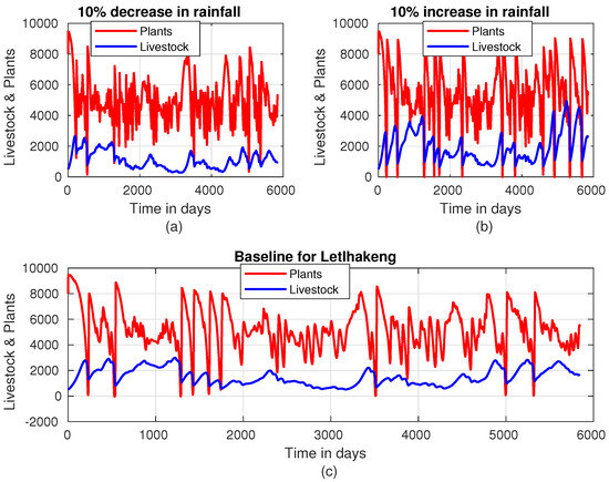
Figure 5.
Plant–livestock population dynamics in Letlhakeng when rainfall intensity is (a) decreased by 10%, (b) increased by 10%, and (c) at baseline.
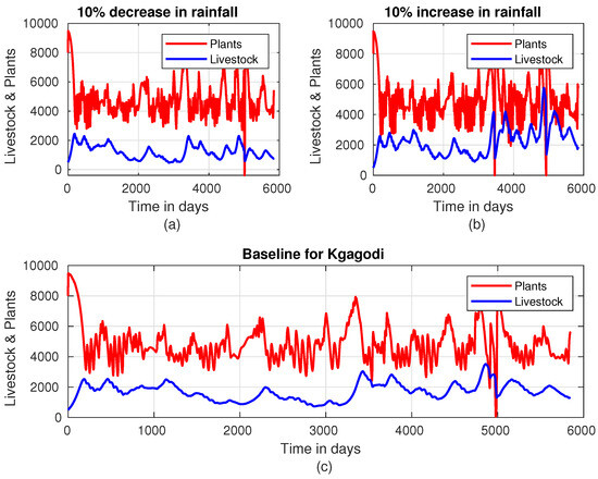
Figure 6.
Plant–livestock population dynamics in Kgagodi when rainfall intensity is (a) decreased by 10%, (b) increased by 10%, and (c) at baseline.
In Sehitlwa Figure 7, the livestock population exhibits a general downward trend starting just after 1000 days, a pattern observed regardless of whether rainfall intensity is increased or decreased. This indicates that other factors, such as competition for resources or natural population dynamics, may contribute to this decline over time.
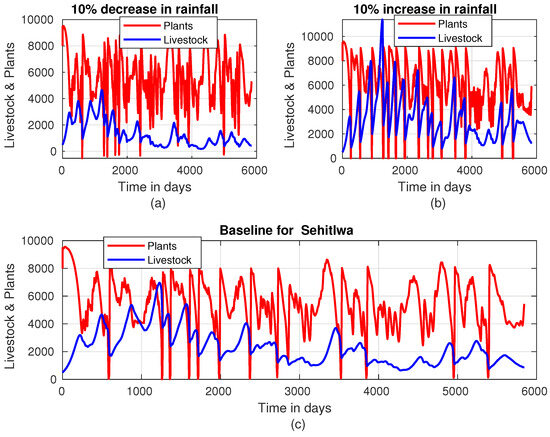
Figure 7.
Plant–livestock population dynamics in Sehitlwa when rainfall intensity is (a) decreased by 10%, (b) increased by 10%, and (c) at baseline.
As depicted in Figure 7, an increase in rainfall intensity by 10% correlates with a significant rise in the average livestock population, approaching a mean of approximately 4000 units of animals. This growth highlights the beneficial impact of enhanced rainfall on both forage availability and livestock productivity. Additionally, vegetation thrives under increased rainfall intensity, supporting the livestock population and providing farmers with ample opportunities for sustainable harvesting. Despite the challenges associated with being situated in a designated red zone area, as noted by [8], farmers still keep livestock in high numbers. The combination of a favorable rainy season and the inflow of water into the Okavango Delta from Angola plays a critical role in maintaining elevated livestock populations in this region, as illustrated in Figure 7, as compared with other areas in the country. Despite the effects of wild animals and floods that usually come around June and August, the land recovers or re-germinates quickly up to its carrying capacity. In Mabutsane, livestock population dynamics are strongly influenced by rainfall intensity (Figure 8). When rainfall intensity decreases, as shown in Figure 8a, livestock numbers predominantly remain below 2000 units. This highlights the region’s vulnerability to reduced rainfall, as lower precipitation directly impacts vegetation growth, thereby limiting the forage available to sustain larger herds.
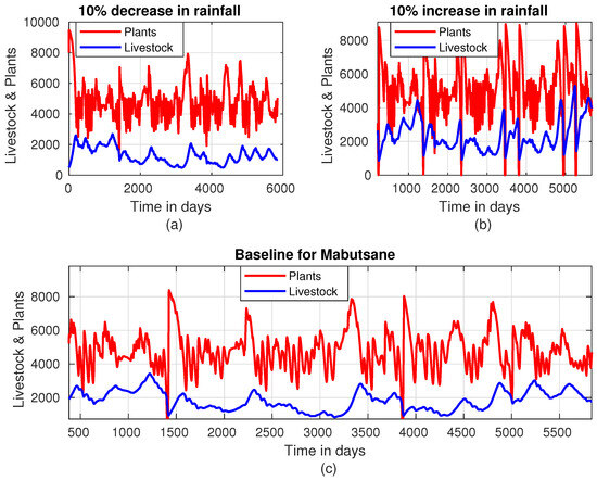
Figure 8.
Plant–livestock population dynamics in Mabutsane when rainfall intensity is (a) decreased by 10%, (b) increased by 10%, and (c) at baseline.
Conversely, as illustrated in Figure 8b, when rainfall intensity is increased by 10%, the livestock population grows significantly, reaching over 4000 units in the later years of the 15-year study period. This increase demonstrates how enhanced rainfall positively impacts forage availability, supporting larger livestock numbers over time. The gradual rise in livestock numbers with increased rainfall also indicates that the ecosystem in Mabutsane has a strong capacity to adapt and expand its carrying capacity under favorable conditions.
3.1.2. Effects of Rainfall Timing in Different Regions of Botswana
In semi-arid areas like Botswana, the rainfall timing significantly affects both plants (forage) and livestock. Timing affects the overall output or harvest of livestock and land vegetation. When considering rainfall timing, it is important to note that the total duration of the rainy season is assumed to remain unchanged in both scenarios (late onset and early onset of the rainy season). For the late onset of the rainy season, seeds may not germinate on time, and existing plants may experience stunted growth or die because of delayed rainfall or a prolonged dry environment [46,47]. This delay in rainfall will lead to a reduction in biomass production, resulting in less food and water available for livestock. These effects on livestock may cause weight loss, decreased milk production, and increased susceptibility to diseases (see [10] and references therein). Additionally, the reduction in forage availability can disturb reproductive cycles, delay breeding, and reduce birth rates. Moreover, when rainfall occurs later than anticipated, specifically 30 days beyond the expected onset, it adversely affects grass growth, leading to stunted growth and reduced biomass, which ultimately results in a temporary shortage of forage. During such periods of delayed rainfall, farmers can start to rely on stored feed or reduce herd sizes to match the available resources [10,48]. This is shown in Figure 9a by a drop in livestock number at day 200. This shows that while some cattle may die, some farmers will start to reduce the number of their livestock to match the available feed. Additionally, others have to start livestock mobility [10], hence reducing the number of livestock. Figure 9 shows that after some time, rain will come, which makes grasses grow again, hence improving reproduction success and leading to higher birth rates and healthier offspring. Consequently, the number of livestock starts to grow again.
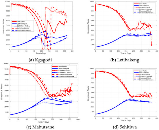
Figure 9.
Figure showing effect of rainfall timing in (a) Kgagodi, (b) Letlhakeng, (c) Mabutsane, and (d) Sehitlwa. The rainfall time is when the rain comes at the expected time; the case is when rain is delayed by 30 days, and lastly, when the rain comes 30 days early.
On the other hand, when rainfall arrives 30 days earlier than expected, the dry period between the previous and current wet seasons will be short, thereby allowing the plant biomass to recover early. This early rainfall also replenishes soil moisture, supporting the growth of deep-rooted plants and making them more resilient to drought stress later in the season. Additionally, the quality of forage is often enhanced, leading to better livestock health, weight gain, and productivity. When rainfall comes early, it reduces the risk of water stress and allows grasses to establish themselves with adequate moisture, providing consistent, high-quality forage for livestock. As a result, livestock benefit from improved nutrition, leading to better overall health, weight gain, and milk production. At the same time, farmers can reduce the need for supplemental feeding, saving costs and resources.
The effects of both delay and early onset of rainfall, as described above, are shown in Figure 9 for each of the four data points and are compared with the baseline value. As observed in Figure 9a,c, there is a significant effect on the livestock population when rain comes early or is delayed as compared with Figure 9b,d. In Figure 9a,c, when rain comes early, the density of livestock reacts well with it, which means their density increases. However, unless it is well managed, this will result in overgrazing in the area, and the livestock population will eventually decrease significantly. That means the advantage will be lost, as can be observed in Figure 9a. On the other hand, when the onset of rainfall is delayed, livestock will not have enough food, which ends up leading to a decrease in the livestock population.
3.1.3. Effect of Harvest Rate ()
In this section, we examine the effect of varying livestock harvest (takeoff) rates in a model where all other parameters are kept constant. Our goal is to understand how the onset of rainfall affects livestock, enabling us to encourage farmers to harvest their livestock strategically to avoid losses due to food shortages, water shortages, and diseases, which are heavily influenced by the timing of rainfall. We analyze how delays or early onset of rainfall impact plant biomass, the primary food source for livestock. This analysis aims to help farmers minimize losses from drought or overgrazing, which are prevalent issues caused by unpredictable rainfall patterns. Such variability in rainfall often results in farmers losing a significant portion of their livestock.
In our model, we assume a threshold of 2000 units of livestock across four regions. When livestock numbers reach or exceed this threshold, farmers are advised to start changing their harvesting strategy. We use a base harvest rate of , suggesting that in a km grid with 500 animals, farmers should harvest at least 32 cattle equivalent livestock over ten years. We maintain consistent initial numbers of livestock and biomass across all four regions while testing various harvest rates: , , , and .
Analyzing the results presented in Figure 10, we observe the effect of an increasing harvest rate when rainfall occurs at the anticipated time, typically at the onset of the spring season in Botswana. Notably, the regions of Sehitlwa, Letlhakeng, and Mabutsane show similar trends in biomass retention. However, Kgagodi’s pattern differs significantly due to lower rainfall levels recorded in 2020, which adversely impact vegetation growth and, thus, livestock sustainability. In Kgagodi, without a harvest rate adjustment, plant biomass is severely affected, especially between days 200 and 250. However, increasing the harvest rate in this region mitigates plant depletion, indicating that by reducing livestock numbers, the remaining animals can be supported by the region’s available resources.
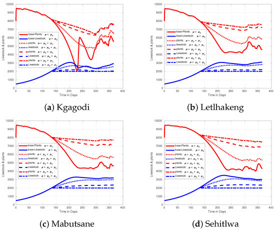
Figure 10.
Figure showing effect of increasing harvest rate when there is no variations in rainfall pattern.
In Kgagodi, where the timing of rainfall has no significant effect, the maximum livestock capacity is around 3000 units. This capacity can only be maintained for a limited duration; if livestock numbers are not carefully managed, there will be a rapid decline. In contrast, other regions are capable of sustaining more than 3000 units for extended periods. Increasing the harvest rate aligns Kgagodi’s biomass patterns more closely with the other regions, indicating that reducing livestock numbers brings them to a sustainable level for the area. This adjustment reduces plant depletion and overgrazing, allowing vegetation to recover and stabilize.
During the late onset of the rainy season, as depicted in Figure 11, livestock in Kgagodi barely reach the 3000-mark, and without harvesting, numbers may drop below 1000. In other regions, livestock levels remain more stable due to sufficient food and water, even with late rains. Increasing the harvest rate in Kgagodi reduces livestock loss, and at a maximum rate of , the region can sustain livestock without significant losses. For the early onset of the rainy period, as shown in, Figure 12, livestock numbers rise to 3000 or more across all regions. In Kgagodi, this increase in livestock population causes severe depletion of plant biomass. Without intervention, livestock could face significant mortality due to food and water shortages, especially during the mid-year. By increasing the harvest rate, fewer livestock remain, thereby reducing the strain on resources and preventing overgrazing. If the harvest rate is not adjusted, Kgagodi could experience losses of up to 1000 animals, resulting in a reduction in over 2000 livestock compared with other regions.
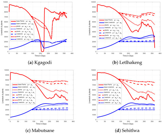
Figure 11.
Figure showing effect of increasing harvest rate when rainfall comes later than expected in different regions of Botswana.
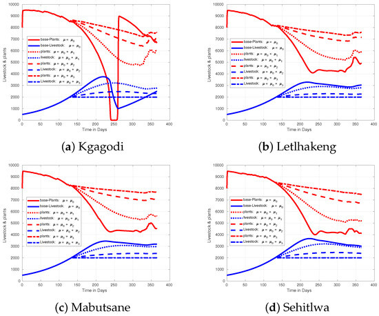
Figure 12.
Figure showing effect of increasing harvest rate when rainfall comes early than expected in different regions of Botswana.
Upon analyzing the plots for Kgagodi in Figure 10, Figure 11 and Figure 12, we observe that the Kgagodi area is particularly sensitive to variations in rainfall timing, with both scenarios showing biomass depletion, especially during mid-year. This depletion strongly impacts livestock, especially when rains are delayed. Increasing the harvest rate here could help stabilize the livestock population by preventing overgrazing during this critical period. Conversely, early rainfall allows for a more consistent supply of biomass, thus better supporting livestock health and productivity. These regions may not require a harvest rate as high as in Kgagodi for livestock management since plant biomass remains more abundant and is able to sustain livestock. However, monitoring is essential to ensure livestock numbers do not exceed the ecosystem’s carrying capacity.
4. Conclusions
This study is primarily motivated by the observed effects of climate variability, with a particular focus on the impact of erratic rainfall patterns on livestock production in Botswana. By estimating relevant model parameters from literature and calculating others using online data, the research demonstrates how fluctuating rainfall directly affects livestock populations. Botswana’s diverse vegetation is classified into four major areas, as shown in Figure 1, with data points Kgagodi, Sehitlwa, Mabutsane, and Letlhakeng, which provides a detailed context for understanding these effects.
The study presents a mathematical model based on a non-autonomous ordinary differential equation that includes a periodic equation for plant growth rates. The model uses rainfall data from Climate Engine (http://ClimateEngine.org, accessed on 15 February 2025) across four distinct study sites to estimate plant growth rates. The model is analyzed for positivity and boundedness. An average reproduction ratio, value, based on the average livestock ratio, for the coexistence of plant and livestock populations was established, and a trapping region was identified. The general pattern of the livestock basic reproduction number is observed to decrease through time. This decrease could be due to some environmental and climatic variations in the region, serving as an important signal to policymakers.
The model’s sensitivity to changes in key parameters such as harvest rate, rainfall intensity (increase or decrease), and the timing of rainfall (early or late onset) was explored. Sensitivity analysis revealed that early rainfall positively impacts livestock production across all regions, as does increased rainfall intensity. Furthermore, adjusting the harvest rate in response to changes in the rainfall pattern significantly enhances livestock management and mitigates overgrazing, demonstrating its importance in maintaining sustainable plant–livestock dynamics.
Numerical simulations underscore that the adverse effects of climatic variations on livestock production can be mitigated by optimizing livestock harvest rates. Increasing the harvest rate reduces livestock numbers, allowing plant biomass to recover and sustain the ecosystem whenever necessary. For example, the analysis of livestock dynamics across different locations highlights the impact of harvesting and rainfall variability on herd numbers. In Kgagodi, without harvesting, livestock numbers decline by approximately 37% due to feed shortages, while moderate harvesting () reduces this loss to 17%. With significant harvesting (), livestock numbers remain stable at their peak levels. In Sehitlwa, biomass declines without harvesting, but livestock numbers show minimal reduction. When rainfall is delayed, Kgagodi experiences a sharper decline (over 55%), with numbers briefly dropping below 1000 before recovering. Letlhakeng, in contrast, sees a 6% increase in livestock when rainfall is delayed, leading to a sharp decrease in biomass, which can be stabilized by harvesting. Mabutsane and Letlhakeng generally maintain their peak numbers with minimal variation. The study shows that in these regions, the growth rate of plants, which serves as the primary food source for livestock, is significantly impacted by inconsistent rainfall. This, in turn, affects the availability of drinking water, resulting in compounding the challenges faced by livestock.
The results align well with observed field data, confirming the physical soundness and applicability of the model. These findings are particularly beneficial for traditional farmers in Botswana, whose livelihoods largely depend on livestock production and who often lack access to advanced climate data or technologies for managing weather variability. The model demonstrates how erratic rainfall patterns, whether characterized by early onset or increased intensity, can enhance plant biomass and, consequently, livestock production. Conversely, delayed rainfall and reduced intensity pose challenges that require strategic management.
Our findings underscore the pressing necessity for the development and implementation of adaptive strategies aimed at mitigating the adverse effects of climate variability on plant–livestock systems in Botswana. It is imperative that policymakers integrate these strategies into agricultural policies, with a focus on promoting sustainable livestock management and environmental conservation. Future research should concentrate on enhancing models that predict livestock production based on rainfall patterns and on investigating the effectiveness of adaptive strategies in diverse regional and contextual settings. While this study is primarily focused on Botswana, its findings possess broader implications, providing valuable insights that can contribute to global efforts to ensure food security and facilitate sustainable agricultural practices in the context of ongoing climate change.
This study also highlights the vital role of adaptable harvest rates in the sustainable management of livestock, particularly in regions such as Kgagodi, where limited rainfall constrains vegetation growth. By adjusting harvest rate practices in accordance with prevailing environmental conditions, we aim to assist farmers in sustaining healthier livestock populations while minimizing the risk of detrimental overgrazing.
Author Contributions
Conceptualization, T.S.N., S.M.K. and G.M.T.; Methodology, S.M.K.; Software, S.M.K.; Formal analysis, T.S.N.; Investigation, T.S.N. and S.M.K.; Resources, S.M.K., M.K. and G.M.T.; Data curation, T.S.N. and S.M.K.; Writing—original draft, T.S.N.; Writing—review & editing, S.M.K., M.K. and G.M.T.; Supervision, S.M.K., M.K. and G.M.T.; Project administration, G.M.T.; Funding acquisition, G.M.T. All authors have read and agreed to the published version of the manuscript.
Funding
This research was funded by O.R. Tambo Africa Research Chairs Initiative as supported by the Botswana International University of Science and Technology, the Ministry of Tertiary Education, Science and Technology; the National Research Foundation of South Africa (NRF); the Department of Science and Innovation of South Africa (DSI); the International Development Research Centre of Canada (IDRC); and the Oliver and Adelaide Tambo Foundation (OATF), with grant number: (UID)136696.
Institutional Review Board Statement
Not applicable.
Informed Consent Statement
Not applicable.
Data Availability Statement
The original contributions presented in the study are included in the article, further inquiries can be directed to the corresponding author.
Conflicts of Interest
The authors declare no conflicts of interest.
References
- Schiess-Meier, M.; Ramsauer, S.; Gabanapelo, T.; König, B. Livestock predation—Insights from problem animal control registers in Botswana. J. Wildl. Manag. 2007, 71, 1267–1274. [Google Scholar] [CrossRef]
- Schlink, A.; Nguyen, M.; Viljoen, G. Water requirements for livestock production: A global perspective. Rev. Sci. Tech. 2010, 29, 603–619. [Google Scholar] [PubMed]
- Seré, C.; Steinfeld, H.; Groenewold, J. World Livestock Production Systems; Food and Agriculture Organization of the United Nations: Rome, Italy, 1996. [Google Scholar]
- Miranda-de la Lama, G.C.; Mattiello, S. The importance of social behaviour for goat welfare in livestock farming. Small Rumin. Res. 2010, 90, 1–10. [Google Scholar]
- Neethirajan, S.; Kemp, B. Digital livestock farming. Sens. Bio Sens. Res. 2021, 32, 100408. [Google Scholar]
- Steinfeld, H. Livestock’s Long Shadow: Environmental Issues and Options; Food & Agriculture Organization: Rome, Italy, 2006. [Google Scholar]
- FAO, Unesco. Global Agriculture Towards 2050. High Level Expert Forum Issues Paper; Food and Agriculture Organization of the United Nations: Rome, Italy, 2009. [Google Scholar]
- Darkoh, M.B.; Mbaiwa, J.E. Globalisation and the livestock industry in Botswana. Singap. J. Trop. Geogr. 2002, 23, 149–166. [Google Scholar]
- Asfaw, M.D.; Kassa, S.M.; Lungu, E.M. Co-existence thresholds in the dynamics of the plant–herbivore interaction with Allee effect and harvest. Int. J. Biomath. 2018, 11, 1850057. [Google Scholar]
- Kgosikoma, O.E. Effects of Climate Variability on Livestock Population Dynamics and Community Drought Management in Kgalagadi, Botswana. Ph.D. Thesis, Norwegian University of Life Sciences, Ås, Norway, 2006. [Google Scholar]
- Moreki, J.; Tsopito, C. Effect of climate change on dairy production in Botswana and its suitable mitigation strategies. Online J. Anim. Feed. Res. 2013, 3, 216–221. [Google Scholar]
- Batisani, N.; Yarnal, B. Rainfall variability and trends in semi-arid Botswana: Implications for climate change adaptation policy. Appl. Geogr. 2010, 30, 483–489. [Google Scholar]
- Ejigu, A.A.; Asfaw, M.D.; Kassa, S.M. Estimating the spatial distribution of possible livestock production level using a mathematical model and the SMAP soil moisture data: The case of Botswana. Commun. Math. Biol. Neurosci. 2022, 2022, 124. [Google Scholar]
- Troiano, C.; Buglione, M.; Petrelli, S.; Belardinelli, S.; De Natale, A.; Svenning, J.C.; Fulgione, D. Traditional free-ranging livestock farming as a management strategy for biological and cultural landscape diversity: A case from the southern apennines. Land 2021, 10, 957. [Google Scholar] [CrossRef]
- Behnke, R.H., Jr. Cattle accumulation and the commercialization of the traditional livestock industry in Botswana. Agric. Syst. 1987, 24, 1–29. [Google Scholar]
- Asfaw, M.D.; Kassa, S.M.; Lungu, E.M.; Bewket, W. Effects of temperature and rainfall in plant–herbivore interactions at different altitude. Ecol. Model. 2019, 406, 50–59. [Google Scholar]
- Kassa, S.M.; Asfaw, M.D.; Ejigu, A.A.; Tsidu, G.M. Modeling natural forage dependent livestock production in arid and semi-arid regions: Analysis of seasonal soil moisture variability and environmental factors. Model. Earth Syst. Environ. 2024, 10, 3645–3663. [Google Scholar]
- Godde, C.M.; Boone, R.B.; Ash, A.J.; Waha, K.; Sloat, L.L.; Thornton, P.K.; Herrero, M. Global rangeland production systems and livelihoods at threat under climate change and variability. Environ. Res. Lett. 2020, 15, 044021. [Google Scholar]
- Kebede, D. Impact of climate change on livestock productive and reproductive performance. Livest. Res. Rural. Dev. 2016, 28, 227. [Google Scholar]
- Sloat, L.L.; Gerber, J.S.; Samberg, L.H.; Smith, W.K.; Herrero, M.; Ferreira, L.G.; Godde, C.M.; West, P.C. Increasing importance of precipitation variability on global livestock grazing lands. Nat. Clim. Change 2018, 8, 214–218. [Google Scholar]
- Giridhar, K.; Samireddypalle, A. Impact of climate change on forage availability for livestock. In Climate Change Impact on Livestock: Adaptation and Mitigation; Springer: New Delhi, India, 2015; pp. 97–112. [Google Scholar]
- Cain, J.W.; Gedir, J.V.; Marshal, J.P.; Krausman, P.R.; Allen, J.D.; Duff, G.C.; Jansen, B.D.; Morgart, J.R. Extreme precipitation variability, forage quality and large herbivore diet selection in arid environments. Oikos 2017, 126, 1459–1471. [Google Scholar]
- Baumgard, L.H.; Rhoads, R.P.; Rhoads, M.L.; Gabler, N.K.; Ross, J.W.; Keating, A.F.; Boddicker, R.L.; Lenka, S.; Sejian, V. Impact of climate change on livestock production. Environ. Stress Amelior. Livest. Prod. 2012, 15, 413–468. [Google Scholar]
- Bekele, S. Impacts of climate change on livestock production: A review. J. Nat. Sci. Res. 2017, 7, 53–59. [Google Scholar]
- Wikipedia Contributors. Statistics Botswana—Wikipedia, The Free Encyclopedia. 2023. Available online: https://en.wikipedia.org/w/index.php?title=Statistics_Botswana&oldid=1151523833 (accessed on 12 June 2023).
- Wikipedia Contributors. Geography of Botswana—Wikipedia, The Free Encyclopedia. 2022. Available online: https://en.wikipedia.org/w/index.php?title=Geography_of_Botswana&oldid=1126000541 (accessed on 12 June 2023).
- Centre for Applied Research. Botswana Country Report ICRISAT-ILRI Project Priorities for Future Research on Crop-Livestock Systems; Final Report December 2005; Government of Botswana: Gaborone, Botswana, 2005.
- Vossen, P. Rainfall and agricultural production in Botswana. Afr. Focus 1990, 6, 141–155. [Google Scholar]
- Barnes, J.I.; Cannon, J.; Macgregor, J. Livestock production economics on communal land in Botswana: Effects of tenure, scale and subsidies. Dev. S. Afr. 2008, 25, 327–345. [Google Scholar]
- Asfaw, M.D.; Kassa, S.M.; Lungu, E.M. Stochastic plant-herbivore interaction model with Allee effect. J. Math. Biol. 2019, 79, 2183–2209. [Google Scholar]
- Bindari, Y.R.; Shrestha, S.; Shrestha, N.; Gaire, T.N. Effects of nutrition on reproduction—A review. Adv. Appl. Sci. Res 2013, 4, 421–429. [Google Scholar]
- Kumar Guntu, R.; Agarwal, A. Investigation of Precipitation Variability and Extremes Using Information Theory. Environ. Sci. Proc. 2020, 4, 14. [Google Scholar] [CrossRef]
- Abrams, P.A.; Ginzburg, L.R. The nature of predation: Prey dependent, ratio dependent or neither? Trends Ecol. Evol. 2000, 15, 337–341. [Google Scholar]
- Sakio, H. Effects of flooding on growth of seedlings of woody riparian species. J. For. Res. 2005, 10, 341–346. [Google Scholar]
- Kneebone, W.; Kopec, D.; Mancino, C. Water requirements and irrigation. Turfgrass 1992, 32, 441–472. [Google Scholar]
- Cho, L.H.; Pasriga, R.; Yoon, J.; Jeon, J.S.; An, G. Roles of sugars in controlling flowering time. J. Plant Biol. 2018, 61, 121–130. [Google Scholar]
- Passioura, J. Soil structure and plant growth. Soil Res. 1991, 29, 717–728. [Google Scholar] [CrossRef]
- Teschl, G. Ordinary Differential Equations and Dynamical Systems; American Mathematical Soc.: Providence, RI, USA, 2012; Volume 140. [Google Scholar]
- Smith, H.L. Monotone Dynamical Systems: An Introduction to the Theory of Competitive and Cooperative Systems: An Introduction to the Theory of Competitive and Cooperative Systems; American Mathematical Soc.: Providence, RI, USA, 1995. [Google Scholar]
- Mberego, S. Temporal patterns of precipitation and vegetation variability over Botswana during extreme dry and wet rainfall seasons. Int. J. Climatol. 2017, 37, 2947–2960. [Google Scholar]
- Puoetsile, A.; Lekgari, M.; Kassa, S.; Tsidu, G.M. Optimized Parameter Estimation and Integrating Neural Network Forecasting of Dynamic Plant-Livestock Model For Early Warning in Agro-Environment Control Systems. Stat. Optim. Inf. Comput. 2024, 12, 1460–1475. [Google Scholar] [CrossRef]
- Botswana, S. Annual Agricultural Survey Report 2019; Traditional Sector; Statistics Botswana: Gaborone, Botswana, 2020. [Google Scholar]
- Terry, A.J. Predator–prey models with component Allee effect for predator reproduction. J. Math. Biol. 2015, 71, 1325–1352. [Google Scholar] [CrossRef] [PubMed]
- Cline, M.G. Basic principles of soil classification. Soil Sci. 1949, 67, 81–92. [Google Scholar] [CrossRef]
- Hempel, J.; Michéli, E.; Owens, P.; McBratney, A. Universal soil classification system report from the International Union of Soil Sciences Working Group. Soil Horizons 2013, 54, 1–6. [Google Scholar] [CrossRef]
- Mphale, K.; Dash, S.; Adedoyin, A.; Panda, S. Rainfall regime changes and trends in Botswana Kalahari Transect’s late summer precipitation. Theor. Appl. Climatol. 2014, 116, 75–91. [Google Scholar] [CrossRef]
- Veenendaal, E.; Ernst, W.; Modise, G. Effect of seasonal rainfall pattern on seedling emergence and establishment of grasses in a savanna in south-eastern Botswana. J. Arid Environ. 1996, 32, 305–317. [Google Scholar] [CrossRef]
- Kenabatho, P.; Montshiwa, M. Integrated water resources management as a tool for drought planning and management in Botswana: A diagnostic approach. Int. J. Sustain. Dev. Plan. 2006, 1, 61–75. [Google Scholar] [CrossRef]
Disclaimer/Publisher’s Note: The statements, opinions and data contained in all publications are solely those of the individual author(s) and contributor(s) and not of MDPI and/or the editor(s). MDPI and/or the editor(s) disclaim responsibility for any injury to people or property resulting from any ideas, methods, instructions or products referred to in the content. |
© 2025 by the authors. Licensee MDPI, Basel, Switzerland. This article is an open access article distributed under the terms and conditions of the Creative Commons Attribution (CC BY) license (https://creativecommons.org/licenses/by/4.0/).