A Unified Denoising Framework for Restoring the LiDAR Point Cloud Geometry of Reflective Targets

Abstract

LiDAR point clouds of reflective targets often contain significant noise, which severely impacts the feature extraction accuracy and performance of object detection algorithms. These challenges present substantial obstacles to point cloud processing and its applications. In this paper, we propose a Unified Denoising Framework (UDF) aimed at removing noise and restoring the geometry of reflective targets. The proposed method consists of three steps: veiling effect denoising using an improved pass-through filter, range anomalies correction through M-estimator Sample Consensus (MSAC) plane fitting and ray projection, and blooming effect denoising based on an adaptive error ellipse. The parameters of the error ellipse are automatically determined using the divergence angle of the laser beam, blooming factors, and the normal vector along the boundary of the point cloud. The proposed method was validated on a self-constructed traffic sign point cloud dataset. The experimental results showed that the method achieved a mean square error (MSE) of 0.15 cm², a mean city-block distance (MCD) of 0.05 cm, and relative height and width errors of 1.92% and 1.91%, respectively. Compared to five representative algorithms, the proposed method demonstrated superior performance in both denoising accuracy and the restoration of target geometric features.

1. Introduction

In recent years, Light Detection and Ranging (LiDAR) technology has undergone rapid development and become a hotspot in both academic research and industrial applications. By emitting pulsed laser beams, LiDAR can quickly capture the three-dimensional spatial information and intensity of surrounding environments. LiDAR demonstrates remarkable advantages under complex scenarios, adverse weather conditions, and varying lighting environments. Consequently, it has been widely used in various applications, such as autonomous driving [1,2,3,4], digital twin city modeling [5,6,7], agricultural monitoring [8,9,10], and forestry surveying [11,12,13].

However, LiDAR systems encounter several critical challenges due to the divergence of the laser beam and the presence of reflective targets (e.g., traffic signs) in complex environments. First, when the laser scans the edges of targets, the signal received by the detector is a mixture of laser echo signals from both the target and the object behind it. This causes the LiDAR system to inaccurately estimate the distance between them, resulting in noise points known as the veiling effect [14]. Second, reflective targets can induce abnormal range measurements, introducing range-anomalous points and reducing feature points on the target surface. Third, the blooming effect [15,16] generates scattered points around the target, leading to distortions in the geometric shape and dimensions of the target. These challenges significantly degrade the performance of object detection and classification algorithms in autonomous driving applications. Consequently, it is still a critical and challenging task to develop effective point cloud denoising algorithms to restore the geometry of reflective targets.

To address these issues, various point cloud denoising methods have been proposed [17,18], which can be categorized into traditional methods [19,20,21,22,23,24,25,26,27,28,29,30,31,32] and deep learning-based methods [33,34,35,36,37,38]. Traditional point cloud denoising methods can further be categorized into filter-based and optimization-based methods.

Filter-based methods [19,20,21,22,23,24,25,26,27,28,29] generally assume that noise is present in high-frequency components and employ filters that function on point positions or normal vectors. The pass-through filter is a simple and effective algorithm in the PCL (Point Cloud Library) [19]; it removes values that are either inside or outside a specified range along a specific dimension (e.g., X, Y, Z coordinates or intensity attribute). Miknis [20,21] improved the computational efficiency of the pass-through filter by optimizing the vector access logic. The statistical filter leverages statistical analysis to remove outliers that are far from their neighbors based on the relative distances between each point and its neighboring points. This method is particularly effective for point clouds with substantial noise or a high presence of outliers. Nurunnabi [22] developed two robust statistical methods for detecting outliers in 3D point cloud data: one leveraging robust z-scores and the other utilizing a robust Mahalanobis distance approach. By incorporating local neighborhood information, the two methods effectively identify both clustered and uniformly distributed outliers. Carrilho [23] introduced an adaptive approach that utilizes point cloud cell subdivision. Rather than generating a single histogram for the entire dataset, the proposed method applies filtering to smaller segments, where variations in ground elevation can be disregarded. The bilateral filter is a technique inspired by the bilateral filter used in image processing, designed to smooth data while preserving edges and geometric features. The method operates by weighting the influence of neighboring points based on both their spatial proximity and feature similarity, such as intensity or surface normal vectors. Fleishman [24] proposed a fast and effective anisotropic mesh denoising algorithm that filters mesh vertices along the normal direction using local neighborhoods. Inspired by the success of bilateral filtering in image denoising, the method extends its principles to 3D meshes, addressing the unique challenges of transitioning from 2D images to 3D manifolds. Digne [25] developed a method that adapts the bilateral filter from grayscale images to 3D meshes, denoising points by considering both spatial proximity and normal direction. This approach achieves effective noise reduction while preserving sharp edges. Wen [26] conducted experimental evaluations of the effectiveness of the point cloud bilateral filtering algorithm in automatic driving scenes. The radius filter identifies and removes outliers in a point cloud by evaluating the number of neighboring points within a specified radius, retaining points only if their neighborhood density meets a predefined threshold. Duan [27] introduced a noise-reduction approach to filtering point clouds, utilizing an adaptive radius outlier removal filter that incorporates principal component analysis. Szutor [28] developed an algorithm inspired by the ROL (Radius Outlier Filter), designed to detect outliers in large-scale point clouds with a non-exponential time complexity. Luo [29] proposed a multibeam point cloud denoising method that combines radius filtering for edge noise removal with density clustering to restore mistakenly filtered terrain points. However, filter-based denoising algorithms are limited by their reliance on predefined parameters and assumptions, making it challenging to balance noise reduction and feature preservation in complex or diverse point cloud datasets.

Optimization-based denoising methods [30,31,32] address the problem by formulating it as an optimization task. The goal is to produce a denoised point cloud that closely aligns with the input data while satisfying constraints derived from prior knowledge of the underlying geometry and noise distribution. However, achieving satisfactory results using these methods often requires careful parameter tuning, especially for complex point cloud structures.

Deep learning-based methods can be classified into supervised [33,34,35] and unsupervised approaches [36,37,38], depending on the availability of labeled data during model training. Deep learning-based techniques eliminate these limitations by learning features directly from the data. Rakotosaona [34] presented a data-driven approach to denoising unordered point clouds, building on the PCPNet framework. The method removes outliers and computes correction vectors to align noisy points with clean surfaces. Luo [38] proposed an algorithm that builds a model to predict a score for each point, representing its significance and helping to differentiate between noise and valid data. Through iterative processing of the initial point cloud, low-score points (noise) are gradually eliminated, while high-score points are preserved. However, supervised approaches typically require large labeled datasets, which are often difficult to obtain. In contrast, unsupervised methods face challenges such as reliance on assumptions about noise characteristics and a limited ability to generalize across diverse LiDAR point cloud datasets.

To remove noise points while preserving features, we developed a Unified Denoising Framework (UDF) for restoring the geometry of reflective targets. The UDF consists of three modules: a veiling effect denoising module, a range anomalies correction module, and a blooming effect denoising module. The performance of the UDF was quantitatively evaluated using a self-constructed traffic sign point cloud dataset. Compared with some traditional and deep learning-based denoising algorithms, the results demonstrated that the proposed framework achieved significant advantages in both denoising performance and geometric feature restoration.

Our contribution in this paper can be summarized in the following three aspects:

(1)

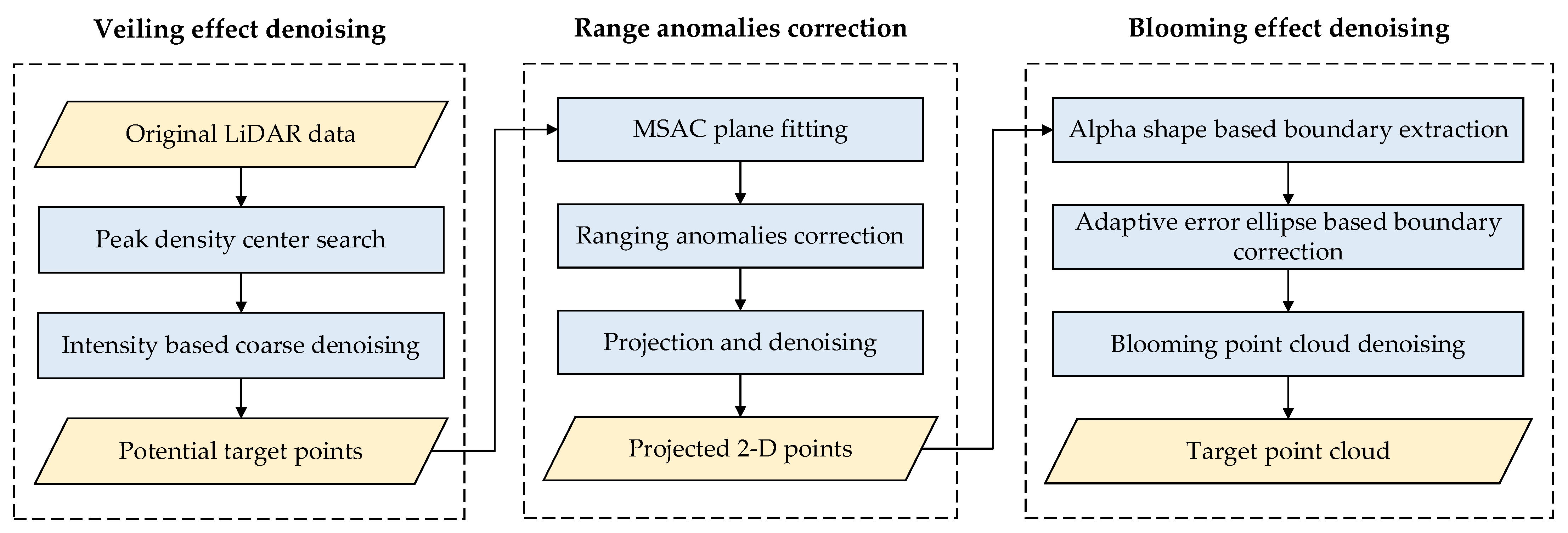
Unlike existing denoising algorithms that typically address only one type of noise, our method is capable of effectively tackling the veiling effect, range anomalies, and blooming effect within a unified framework, offering a comprehensive solution to the challenges encountered in complex scenarios.

(2)

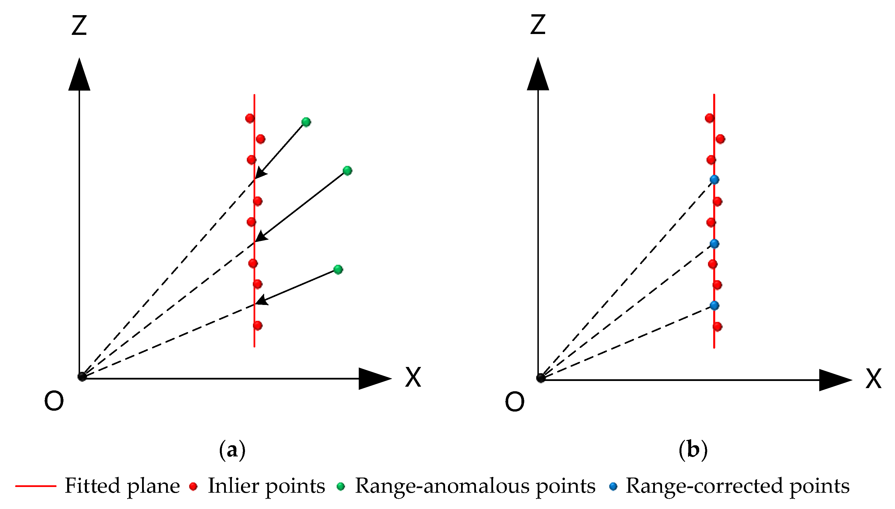
By integrating the MSAC-based plane fitting algorithm with a ray-projection approach, the range-anomalous points are corrected back to the fitted plane. Compared with denoising algorithms based on spatial statistical strategies, which tend to treat these points as noise and remove them, our method recovers these points to the target’s surface, resulting in a denser and more complete point cloud representation.

(3)

To the best of our knowledge, our method is the first to utilize the spatial energy distribution of Gaussian laser beams to eliminate noise points caused by the blooming effect. An adaptive error ellipse is used to refine the boundary of the blooming point cloud. The parameters of the error ellipse are adaptively determined based on the divergence angle of the laser beam, the target distance, and the normal vector along the boundary. With simple adjustments to the algorithm’s parameters, it can be applied to various LiDAR models with different divergence angles.

The rest of this paper is organized as follows: Section 2 provides a detailed introduction to the dataset and the proposed denoising framework. Section 3 presents the experiments and results, including experimental setup, evaluation metrics, and experimental results. Section 4 discusses the proposed algorithm, and the conclusions are summarized in Section 5.

2. Materials and Methods

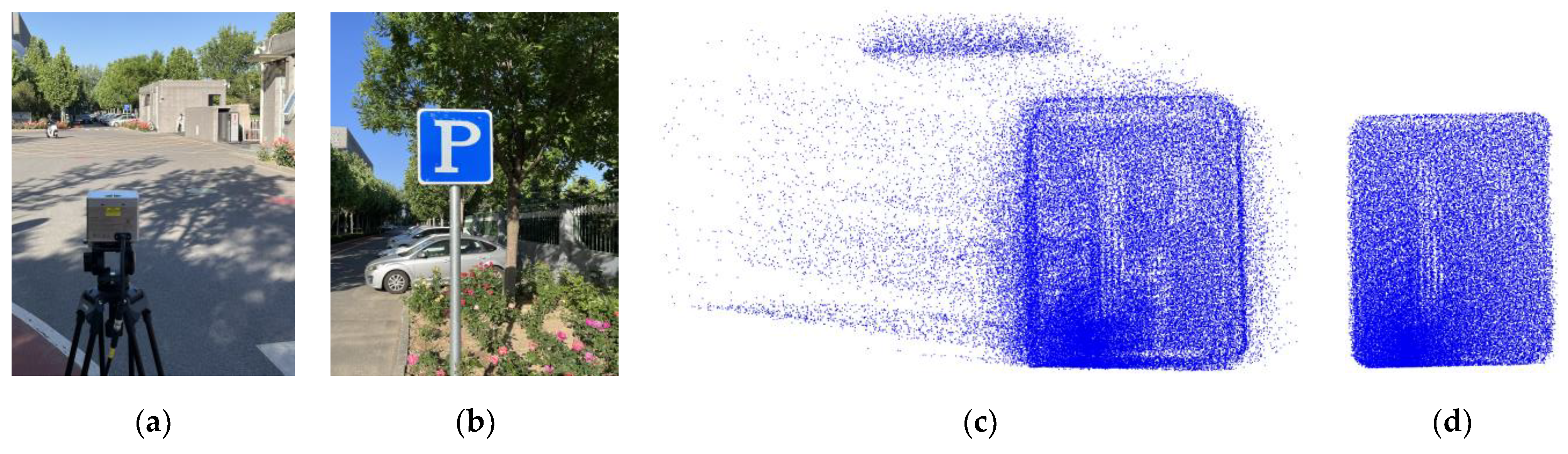
2.1. Dataset

The dataset used in this study was collected using the DJI Livox (Shenzhen, China) Tele-15 LiDAR sensor, which operates at a laser wavelength of 905 nm, with a range precision (1σ @ 20 m) of 2 cm and a laser beam divergence half-angle of 0.12° (vertical) × 0.02° (horizontal). The reflective target used for data acquisition was a square traffic sign with dimensions of 0.6 m × 0.6 m. Due to the non-repetitive scanning characteristics of the Tele15 sensor, the point cloud density varied across different positions within the sensor’s scanning area. To better simulate the diversity of data encountered in autonomous driving scenarios, we considered several factors during data collection, including variations in lighting conditions, target distance, laser incidence angle, and point cloud density at different target locations. Data were collected at 14 distinct distances under varying lighting conditions. During data acquisition at each distance, the LiDAR sensor was mounted on a tripod, and its orientation was adjusted to change both the position of the target within the sensor’s field of view and the laser incidence angle on the target surface. At each distance, 90 samples were acquired, resulting in 1260 samples in total in the dataset.

The data acquisition scenario and point cloud are shown in Figure 1. The ground-truth point cloud of the target in each sample was obtained through manual editing and programmatic processing, incorporating prior knowledge of the target’s geometric shape and dimensions.

2.2. Methods

The proposed method uses a unified framework to remove noise points of reflective targets. The workflow consists of three main parts, as illustrated in Figure 2. First, original LiDAR data are preprocessed to remove points caused by the veiling effect, which are usually with a low intensity, thereby identifying potential target points. The intensity threshold is determined by locating the peak probability density center. Second, the MSAC algorithm is applied to extract a plane and classify points as inliers and outliers. Subsequently, noise points with range anomalies are corrected back to the target’s surface, followed by the projection of the point cloud onto the YOZ plane and the removal of isolated noise points. Third, boundary extraction is performed using the alpha shape algorithm, followed by point-wise boundary correction based on an adaptive error ellipse to refine the boundary. The parameters of the error ellipse are automatically adjusted according to the target’s distance and the normal vector along the original boundary. Finally, noise points caused by the blooming effect are removed using both the original and the newly refined boundaries, ensuring an accurate restoration of the geometry of the target.

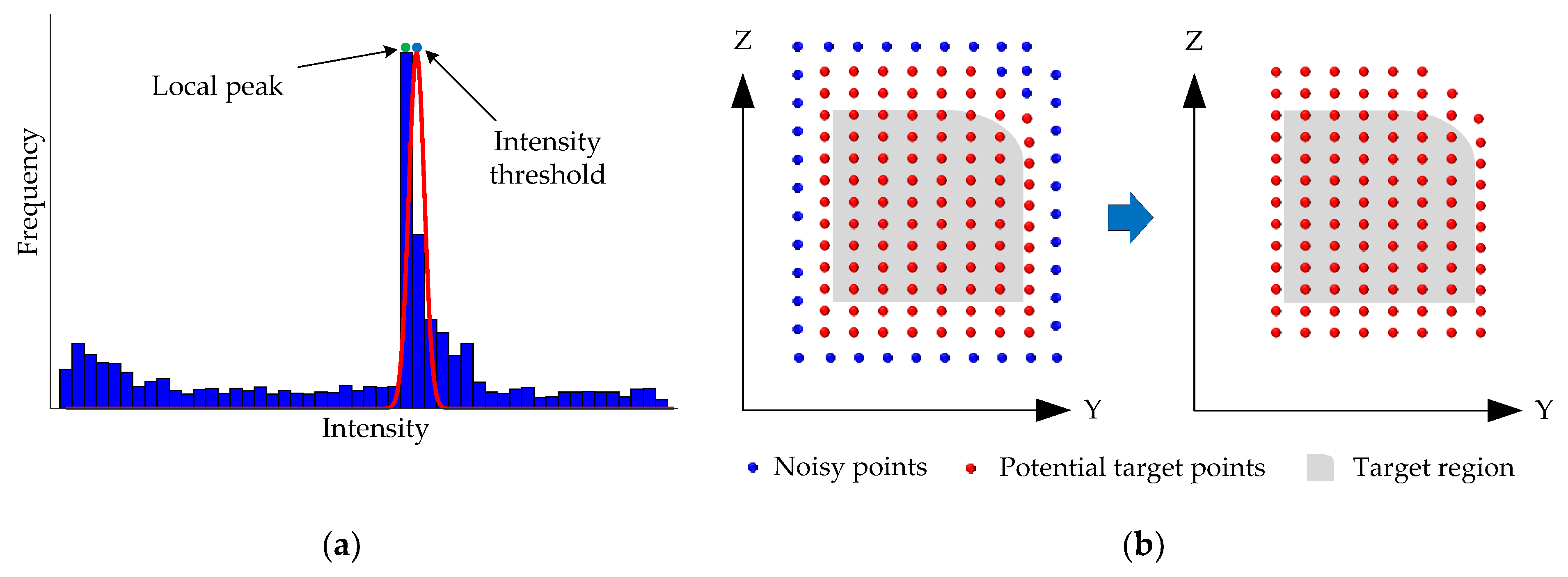
2.2.1. Veiling Effect Denoising

The original LiDAR point cloud data contain a large number of noise points induced by the veiling effect, which are usually located near the edges of the target. These noise points share a common characteristic of a relatively low reflectivity intensity. To remove these noise points, we employ an improved intensity-based pass-through filtering algorithm, as illustrated in Figure 3.

The intensity threshold for the pass-through filter is determined by searching for the center of the peak probability density. First, the intensity of all points is statistically analyzed. Then, a local peak detection algorithm [39] is applied to identify the local peaks in the histogram, and the peak with the highest intensity is selected. Subsequently, Gaussian fitting [40] is performed on the data within the neighborhood of this peak to determine the center point of the local distribution. Finally, the intensity of the center point is used as the threshold to remove all points with an intensity below this value, leaving the remaining points as potential target points.

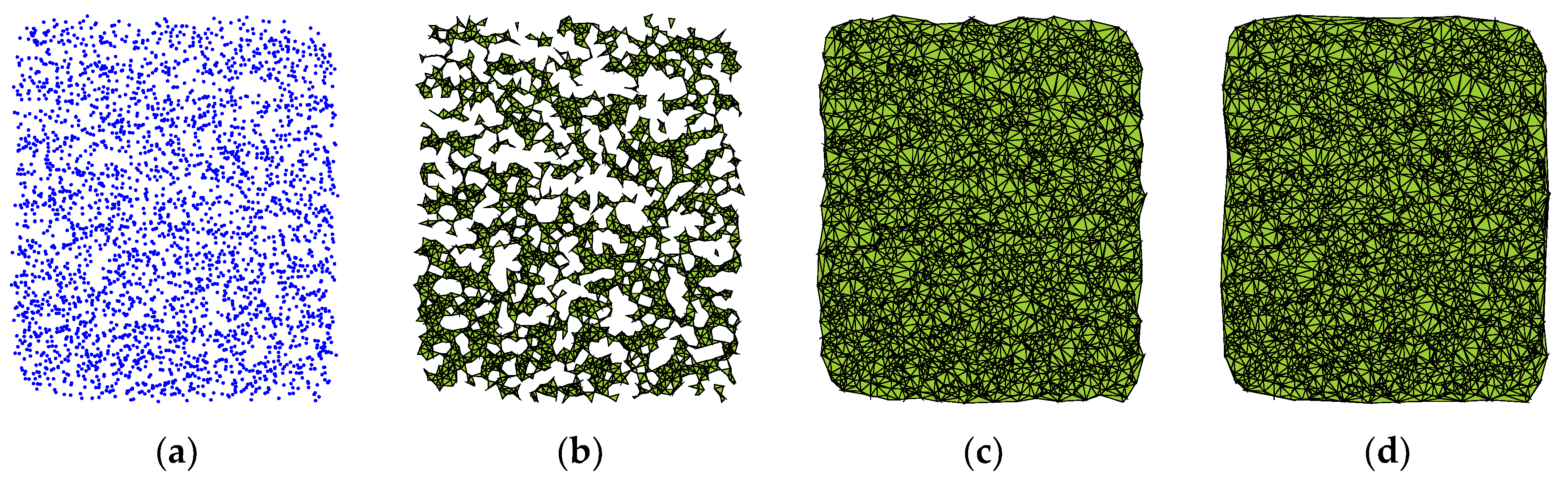
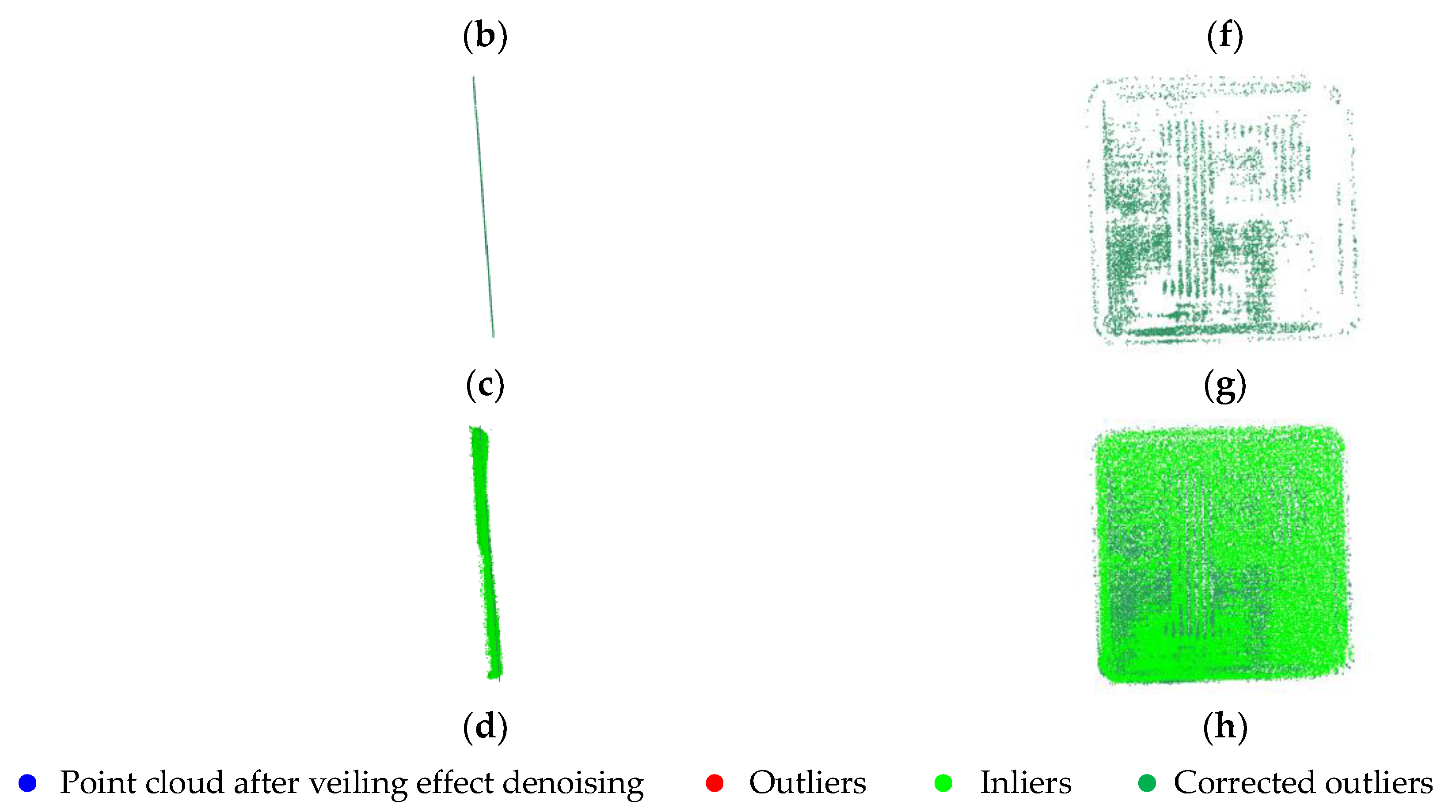
2.2.2. Range Anomalies Correction

Random sample consensus (RANSAC) [41] identifies inlier data and fits a model by searching for the minimum cost under the given model and distance threshold. A point is classified as an inlier with a weight of zero if its distance to the model is less than the threshold; otherwise, it is classified as an outlier. Since all inliers have a weight of zero, the algorithm selects the optimal model with the maximum number of inliers and the smallest total weight. However, when the threshold is set too large, especially for datasets containing distinct outliers, it may result in a significant increase in fitting errors.

MSAC [42] is an improved variant of the RANSAC algorithm designed to reduce the algorithm’s sensitivity to the selection of the distance threshold T. The modified cost function is shown in Equation (1). When the distance e from a point to the model is less than the threshold T, the point is classified as an inlier and assigned a weight of e. Otherwise, the point is classified as an outlier and assigned a weight of T.

$${\mathsf{\rho }}_2(e^2)=\left\{\begin{array}{cc}{e}^2\hfill & e^2<T^2\hfill \\ T^2\hfill & e^2\ge T^2\hfill \end{array}\right.$$

(1)

Due to the signal saturation and distortion of the pulsed laser echo when measuring the surface of reflective targets, measurement errors cause a shift in the distance along the direction of laser emission. This results in the loss of certain surface features of the target. Therefore, although the spatial distribution characteristics of outliers are similar to those of noise points caused by the veiling effect, their intensity values are nearly identical to those of the point cloud on the surface of the reflective target. Based on the principles of range anomalies described above, the outliers are processed as follows: first, the laser emission vector is obtained by connecting the origin of the LiDAR coordinate system to the range-anomalous point; then, the intersection of this vector with the plane fitted by MSAC is calculated. The intersection point (Equation (2)) represents the corrected position of the outlier. The illustration of the range-anomalous points’ correction is shown in Figure 4; the procedure of the algorithm is presented in Algorithm 1.

$$\left\{\begin{array}{c}{x}_0\prime =-{\displaystyle \frac{d_0}{a_0{x}_0+b_0{y}_0+c_0{z}_0}}\cdot x_0\\ y_0\prime =-{\displaystyle \frac{d_0}{a_0{x}_0+b_0{y}_0+c_0{z}_0}}\cdot y_0\\ z_0\prime =-{\displaystyle \frac{d_0}{a_0{x}_0+b_0{y}_0+c_0{z}_0}}\cdot z_0\end{array}\right.$$

(2)

where $(x_0,y_0,z_0)$ and $(x_0\prime ,y_0\prime ,z_0\prime )$ represent the coordinates of the range-anomalous point and the range-corrected point, respectively. The parameters a₀, b₀, c₀, and d₀ are the coefficients of the plane equation $a_{0}x+b_{0}y+c_{0}z+d_0=0$.

Algorithm 1: The range anomalies correction algorithm

Input: Potential target points $P$ and the maximum distance from an inlier point to the plane $d_{\max }$ Output: Projected 2D points $Q$ (1)  Fit a plane to $P$ using the MSAC algorithm to obtain the plane equation. (2)  Classify points as inliers $P_{in}$$\mathrm{and} \mathrm{outliers} P_{out}$ (3)  $\mathbf{if} P_{out}$ is not empty then (4)     $\mathbf{for} \mathrm{each} \mathrm{point} P_i\in P_{out}$ do (5)        Define the origin of the LiDAR coordinate system as O (0, 0, 0) (6)        $\mathrm{Compute} \mathrm{the} \mathrm{vector} \mathrm{of} \overrightarrow{O{P}_i}$ (7)        $\mathrm{Compute} \mathrm{intersection} P_i\prime$$\mathrm{of} \overrightarrow{O{P}_i}$ with the plane a0x + b0y + c0z + d0 = 0 (8)        $\mathrm{Update} P_i$$\mathrm{with} P_i\prime$ (9)     end for (10)  end if (11)  $\mathrm{Combine} \mathrm{inliers} \mathrm{and} \mathrm{corrected} \mathrm{outliers} \mathrm{and} \mathrm{get} P\prime$ (12)  $\mathrm{Project} \mathrm{all} \mathrm{points} \mathrm{in} P\prime$ onto the YOZ plane and remove isolated noise points (13)  return $Q$

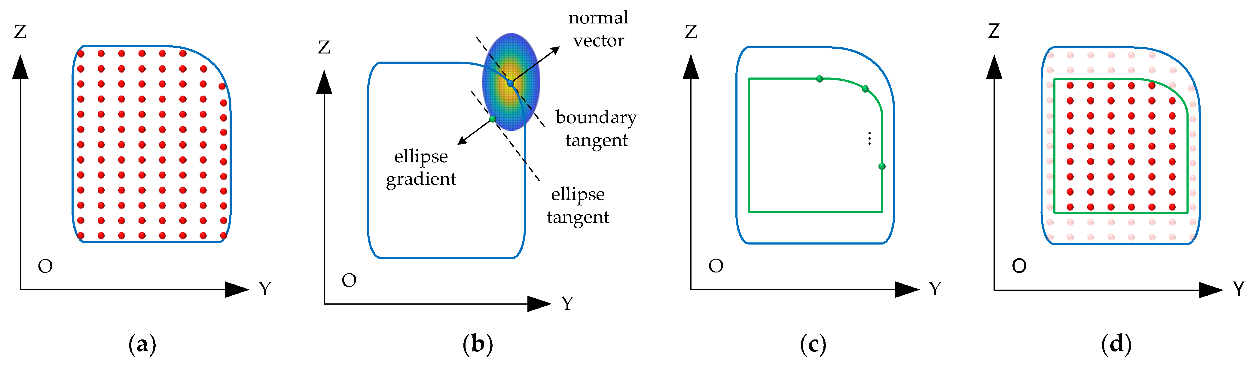
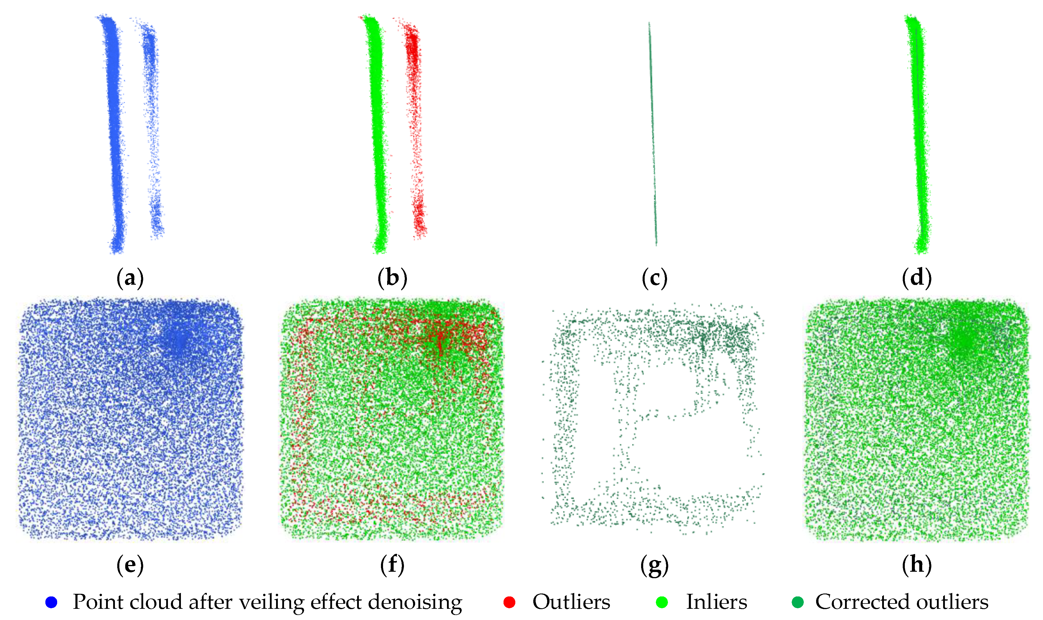
2.2.3. Blooming Effect Denoising

The workflow of the blooming effect denoising algorithm is illustrated in Figure 5, and the detailed procedure is outlined in Algorithm 2. For the point cloud projected onto the YOZ plane after correcting range anomalies, the denoising process involves the following steps:

• Boundary extraction: Use the alpha shape algorithm to extract the boundary of the point cloud, obtaining boundary segments and boundary points.
• Error ellipse construction: Construct an error ellipse centered at each boundary point. The length of the semi-major and semi-minor axes of the ellipse (Equation (3)) are determined based on the LiDAR beam divergence angle (${\theta }_V$ and ${\theta }_H$), target distance ($L$), and blooming factors (${\lambda }_V$ and ${\lambda }_H$). The blooming factors can be estimated through a simple experiment: collect point cloud data of a target with known dimensions at a specific distance and compare the size of the point cloud with the actual size of the target to estimate the factors. In the equation, the subscripts $V$ and $H$ represent vertical and horizontal, respectively.

  $$\left\{\begin{array}{c}a=L\cdot \tan ({\theta }_V)\cdot {\lambda }_V\\ b=L\cdot \tan ({\theta }_H)\cdot {\lambda }_H\end{array}\right.$$

  (3)
• Normal vector calculation: For each boundary point, compute the normal vectors of its adjacent left and right boundary segments. The normalized sum of these two vectors is used as the normal vector (Equation (4)) of the boundary point.

  $$\overrightarrow{\mathit{v}}=(v_y,v_z)$$

  (4)
• Boundary point correction: Draw the tangent and the normal vector at each boundary point. Adjust the tangent along the direction of the normal vector until it is tangential to the error ellipse. The point of tangency is regarded as the corrected boundary point $(y_t,z_t)$. The gradient unit vector of the ellipse at this point is $\overrightarrow{\mathit{G}}$ (Equation (5)). Let $\overrightarrow{\mathit{v}}=\overrightarrow{\mathit{G}}$; then, the absolute value of the slope of the line connecting this point to the center of the ellipse can be obtained (Equation (6)). The absolute value of the boundary point coordinate offset is shown in Equation (7).

  $$\overrightarrow{\mathit{G}}=({\displaystyle \frac{2y_t}{b^2}},{\displaystyle \frac{2z_t}{a^2}})$$

  (5)

  $$k=\left|{\displaystyle \frac{v_z}{v_y}}\right|\cdot {\displaystyle \frac{a^2}{b^2}}$$

  (6)

  $$\left\{\begin{array}{c}\left|\Delta y\right|={\displaystyle \frac{ab}{\sqrt{a^2+b^2{k}^2}}}\\ \left|\Delta z\right|={\displaystyle \frac{kab}{\sqrt{a^2+b^2{k}^2}}}\end{array}\right.$$

  (7)
• Noise removal: Traverse all boundary points of the original point cloud to generate a new refined boundary. Points located between the original boundary and the corrected boundary are identified as noise and are removed.

In this study, the alpha shape algorithm [43] was used to extract the boundary of the point cloud. The basic idea of alpha shape is to describe the shape of a point set by adjusting the parameter $\mathsf{\alpha }$, which serves as a generalization of the convex hull. Alpha shape utilizes Delaunay triangulation to construct the geometric structure of the points and uses $\mathsf{\alpha }$ to control the level of detail in the shape. When α is large, the result approximates the convex hull; when α is small, it captures more detailed local features. As illustrated in Figure 6, when the alpha radius is small, the algorithm can capture fine and complex local details, but the extracted boundary contours tend to be complex and fragmented. As the alpha radius increases, the extracted boundary contours gradually become smoother.

As the target distance increases, the point cloud becomes sparser. To address this, we adopt the average point spacing of the point cloud projected onto the YOZ plane as the alpha radius, ensuring adaptability for boundary extraction across targets at varying distances.

Algorithm 2: The boundary correction algorithm based on adaptive error ellipse

Input: Projected 2D points $Q$ and alpha radius ${\mathsf{\alpha }}_r$ Output: Target points $T$ (1)  Extract the boundary of point cloud $Q$ using alpha shape with alpha radius ${\mathsf{\alpha }}_r$ (2)  Obtain the facets $F$ (each facet represents an edge segment in a 2D plane) and the corresponding boundary points $B$ (each facet contains two boundary points) (3)  Initialize the normal vector for each boundary point with zero values (4)  for each facet $f_i\in F$ do (5)      Compute the normal vector $\overrightarrow{{\mathit{n}}_{\mathit{i}}}$ for the facet $fi$ using its two endpoints $b_i$ and $b_j$ (6)      Normalize $\overrightarrow{{\mathit{n}}_{\mathit{i}}}$ to make it a unit vector (7)      Accumulate $\overrightarrow{{\mathit{n}}_{\mathit{i}}}$ to the normal of the two endpoints $b_i$ and $b_j$ (8)  end for (9)  Initialize the corrected boundary points with $B$ (10)  for each boundary point $b_i\in B$ do (11)     Compute the unit normal vector $\overrightarrow{{\mathit{v}}_{\mathit{i}}}$ for the point $b_i$ (12)     Compute the distance L from $b_i$ to the origin of the LiDAR coordinate system (13)     Define the adaptive error ellipse centered at $b_i$; calculate the semi-major axis a and semi-minor axis b of the ellipse (14)     Calculate the absolute value of the slope k between the original boundary point and the corrected boundary point $b_i\prime$ (15)     Calculate the corrected boundary point coordinate $b_i\prime$ based on the adaptive ellipse parameters (16)  end for (17)  Connect all points $b_i\prime$ to form the new boundary (18)  for each point $q\in Q$ do (19)     if $q$ is located between the original and the corrected boundaries, then (20)        Mark $q$ as an inflated point and remove it (21)     else if $q$ is located inside the corrected boundary, then (22)        Mark $q$ as a target point and retain it (23)  end if (24)  return $T$

3. Experiments and Results

3.1. Experimental Setup

The proposed algorithm was implemented in MATLAB R2022b, and the experiments were performed on a desktop computer equipped with an Intel(R) Core(TM) i7-12700H CPU @2.30 GHz and 64 GB of RAM (Lenovo, Beijing, China). A suite of minimal bounding objects available on the MATLAB Community File Exchange was employed to compute minimal bounding geometries, including circles, rectangles, triangles, and spheres. The Inspector module of PolyWorks Metrology Suite was utilized for the visualization of point cloud data.

3.2. Evaluation Metrics

To evaluate the denoising performance of the proposed algorithm, we employed four metrics derived from the confusion matrix of the denoising results (see

Table 1. Confusion matrix for the LiDAR point cloud denoising results.

		Denoised Data
		Target Points	Noise Points
Ground-Truth	Target points	TP	FN
	Noise points	FP	TN

Note: TP, TN, FP, and FN refer to True Positive, True Negative, False Positive, and False Negative, respectively, representing the correctly and incorrectly classified targets and noise points.

), which have been commonly applied in previous studies [44]. These metrics include the type I error (T.I), type II error (T.II), total error (T.E.), and kappa coefficient (κ). The type I error (Equation (8)) represents the percentage of target points incorrectly classified as noise points, while the type II error (Equation (9)) reflects the proportion of noise points mistakenly classified as target points. The total error (Equation (10)) quantifies the overall proportion of misclassified points. Meanwhile, the kappa coefficient (Equation (11)) provides an alternative metric for accessing overall classification accuracy by accounting for chance agreement and quantifying the improvement in classification accuracy over a random classification.

$$Type I error={\displaystyle \frac{FN}{TP+FN}}$$

(8)

$$Type II error={\displaystyle \frac{FP}{FP+TN}}$$

(9)

$$Total error={\displaystyle \frac{FN+FP}{S}}$$

(10)

$$Kappa coefficient={\displaystyle \frac{p_0-p_e}{1-p_e}}$$

(11)

where $S=TP+FN+FP+TN$, $p_0={\displaystyle \frac{TP+TN}{S}}$, $p_e={\displaystyle \frac{(TP+FN)(TP+FP)+(FP+TN)(FN+TN)}{S^2}}$.

Additionally, to evaluate the performance of the proposed algorithm in restoring the geometric features of reflective targets, four metrics were introduced: mean square error (MSE), mean city-block distance (MCD), relative height error (R.H), and relative width error (R.W). These metrics are designed to evaluate the geometric fidelity of the point cloud, with a focus on spatial accuracy and dimensional consistency [45].

Suppose the ground-truth point cloud and the restored point cloud are $P={\left\{{\mathit{p}}_i\right\}}_{i=1}^{N_1}$, $Q={\left\{{\mathit{q}}_i\right\}}_{i=1}^{N_2}$, where ${\mathit{p}}_i,{\mathit{q}}_i\in {ℝ}^3$. It should be noted that $N_1$ and $N_2$ are not necessarily equal. First, we calculate the average squared Euclidean distance from each ground-truth point to its closest restored point and vice versa: from each restored point to its closest ground-truth point. The final MSE value (Equation (12)) is derived by averaging these two measures, providing a quantitative measure of the discrepancy between the ground-truth points and the restored points. The MCD (Equation (13)) is calculated in a similar manner to the MSE, but it employs the $l_1$ norm in place of the $l_2$ norm.

$$MSE={\displaystyle \frac{1}{2}}\left({\displaystyle \frac{{\displaystyle \sum _{{\mathit{p}}_i\in P}\underset{{\mathit{q}}_j\in Q}{\min }}{‖{\mathit{p}}_i-{\mathit{q}}_j‖}_2^2}{N_1}}+{\displaystyle \frac{{\displaystyle \sum _{{\mathit{q}}_i\in Q}\underset{{\mathit{p}}_j\in P}{\min }}{‖{\mathit{q}}_i-{\mathit{p}}_j‖}_2^2}{N_2}}\right)$$

(12)

$$MCD={\displaystyle \frac{1}{2}}\left({\displaystyle \frac{{\displaystyle \sum _{{\mathit{p}}_i\in P}\underset{{\mathit{q}}_j\in Q}{\min }}\left|{\mathit{p}}_i-{\mathit{q}}_j\right|}{N_1}}+{\displaystyle \frac{{\displaystyle \sum _{{\mathit{q}}_i\in Q}\underset{{\mathit{p}}_j\in P}{\min }}\left|{\mathit{q}}_i-{\mathit{p}}_j\right|}{N_2}}\right)$$

(13)

The actual height (H) and width (W) of the target are first measured using a ruler. Subsequently, the height (h) and width (w) of the restored point cloud are calculated. The relative error (Equations (14) and (15)) is defined as the ratio of the absolute difference between the calculated and actual values to the actual values.

$$relative height error={\displaystyle \frac{\left|H-h\right|}{H}}$$

(14)

$$relative width error={\displaystyle \frac{\left|W-w\right|}{W}}$$

(15)

where $H$ and $W$ refer to the height and width of targets in the denoised point cloud, while $h$ and $w$ denote the actual height and width of the target.

3.3. Experimental Results

To evaluate the algorithm’s performance, we randomly selected one sample from each of the 14 distances in the dataset. The denoising results of the UDF for 14 samples are summarized in

Table 2. Performance evaluations of the UDF on the self-constructed dataset.

Sample	T.I (%)	T.II (%)	T.E (%)	Kappa (%)	MSE (cm2)	MCD (cm)	R.H (%)	R.W (%)
Sample 1	2.59	2.10	2.47	93.32	0.02	0.05	0.40	3.12
Sample 2	0.06	5.74	2.22	95.24	0.03	0.06	1.25	2.78
Sample 3	0.01	4.53	1.85	96.14	0.02	0.02	1.53	2.01
Sample 4	0.01	3.73	1.64	96.66	0.02	0.02	1.40	1.57
Sample 5	0.41	3.20	1.73	96.52	0.03	0.02	1.65	2.47
Sample 6	0.42	3.33	1.87	96.26	0.06	0.03	2.29	0.16
Sample 7	0.42	3.91	2.29	95.40	0.07	0.04	3.19	2.08
Sample 8	0.43	0.42	0.42	99.15	0.02	0.01	0.12	0.52
Sample 9	0.44	5.54	3.51	92.78	0.17	0.07	5.00	4.05
Sample 10	0.01	1.27	0.79	98.33	0.06	0.02	0.69	1.25
Sample 11	1.05	2.76	2.16	95.32	0.17	0.06	2.86	2.35
Sample 12	2.76	0.85	1.50	96.65	0.11	0.05	1.42	0.85
Sample 13	4.56	2.89	3.45	92.29	0.12	0.04	0.42	2.03
Sample 14	6.94	1.60	3.40	92.32	1.18	0.23	4.60	1.51
Avg.	1.44	2.99	2.09	95.46	0.15	0.05	1.92	1.91
Max.	6.94	5.74	3.51	99.15	1.18	0.23	5.00	4.05
Min.	0.01	0.42	0.42	92.29	0.02	0.01	0.12	0.16
Std.	2.01	1.58	0.89	2.05	0.29	0.05	1.46	1.01

. The algorithm achieved an overall average total error of 2.09% and a kappa coefficient of 95.46%, with standard deviations of 0.89% and 2.05%, respectively. These results demonstrate the algorithm’s robust performance and high classification accuracy across targets at varying distances and orientations.

For the MSE and MCD metrics, the average values across all samples were 0.15 cm² and 0.05 cm, respectively. Notably, Sample 14 exhibited the highest MSE and MCD values, likely due to its longer distance, which resulted in a sparser point cloud. This sparsity appears to have negatively impacted the accuracy of target boundary extraction during the blooming effect denoising step. The average relative height error and relative width error across all samples were approximately 1.9%. For a target with dimensions of 60 cm in height and width, this corresponds to absolute errors in height and width not exceeding 2 cm.

To compare the proposed framework with previous point cloud denoising approaches, we selected five representative methods from recent years, including four traditional denoising algorithms and one deep learning-based algorithm. Some algorithms adjust the spatial positions of the original point cloud during the denoising process, making it difficult to calculate total error and kappa coefficient. Therefore, we selected MSE, MCD, relative height error, and relative width error as metrics to evaluate the feature preservation and recovery capabilities of the algorithms.

The results for MSE and MCD are presented in

Table 3. MSE comparison among algorithms (cm²).

Sample	Rusu [19]	Nurunnabi [22]	Digne [25]	Rakotosaona [34]	Duan [27]	Ours
Sample 1	238.28	2.00	223.48	238.34	1.52	0.02
Sample 2	5.77	2.30	10.01	5.87	2.02	0.03
Sample 3	0.73	0.37	9.77	0.73	0.73	0.02
Sample 4	1.18	0.63	10.15	1.18	1.13	0.02
Sample 5	1.74	1.03	9.72	1.74	1.56	0.03
Sample 6	2.68	1.40	10.26	2.68	2.47	0.06
Sample 7	3.62	2.32	9.86	3.62	3.30	0.07
Sample 8	5.17	3.02	10.57	5.17	4.68	0.02
Sample 9	6.81	4.44	9.49	6.81	5.65	0.17
Sample 10	10.88	6.43	12.41	10.88	9.05	0.06
Sample 11	12.45	6.35	11.33	12.45	8.58	0.17
Sample 12	18.57	13.44	14.52	18.57	16.17	0.11
Sample 13	16.67	8.74	13.52	16.67	12.08	0.12
Sample 14	24.81	13.09	19.46	24.81	19.94	1.18
Avg.	24.95	4.68	26.75	24.97	6.35	0.15
Max.	238.28	13.44	223.48	238.34	19.94	1.18
Min.	0.73	0.37	9.49	0.73	0.73	0.02
Std.	59.58	4.23	54.63	59.60	5.84	0.29

Note: The bolded numbers represent the lowest MSE values for each sample.

and

Table 4. MCD comparison among algorithms (cm).

Sample	Rusu [19]	Nurunnabi [22]	Digne [25]	Rakotosaona [34]	Duan [27]	Ours
Sample 1	3.16	0.16	5.21	3.24	0.13	0.05
Sample 2	0.70	0.34	1.86	0.89	0.43	0.06
Sample 3	0.21	0.14	1.77	0.21	0.40	0.02
Sample 4	0.28	0.20	1.85	0.28	0.49	0.02
Sample 5	0.36	0.27	1.80	0.37	0.54	0.02
Sample 6	0.48	0.34	1.93	0.48	0.75	0.03
Sample 7	0.59	0.47	1.88	0.59	0.87	0.04
Sample 8	0.74	0.55	2.04	0.74	1.01	0.01
Sample 9	0.89	0.72	1.81	0.89	1.09	0.07
Sample 10	1.18	0.87	2.27	1.18	1.51	0.02
Sample 11	1.26	0.85	2.21	1.26	1.37	0.06
Sample 12	1.63	1.34	2.48	1.63	1.96	0.05
Sample 13	1.49	1.02	2.46	1.49	1.67	0.04
Sample 14	1.85	1.20	3.21	1.85	2.17	0.23
Avg.	1.06	0.61	2.34	1.08	1.03	0.05
Max.	3.16	1.34	5.21	3.24	2.17	0.23
Min.	0.21	0.14	1.77	0.21	0.13	0.01
Std.	0.77	0.38	0.88	0.78	0.61	0.05

Note: The bolded numbers represent the lowest MCD values for each sample.

. As shown, the UDF achieved the highest accuracy across all samples, which is primarily due to its precise recovery of range-anomalous points and its effective denoising of the blooming effect. In contrast, other algorithms, which treat range-anomalous points as noise and are less effective at denoising the blooming effect, exhibited higher MSE and MCD values.

The evaluation results for relative height error and relative width error are presented in

Table 5. Relative height error comparison among algorithms (%).

Sample	Original Data	Rusu [19]	Nurunnabi [22]	Digne [25]	Rakotosaona [34]	Duan [27]	Ours
Sample 1	42.27	36.48	4.86	9.39	35.80	3.56	0.40
Sample 2	62.33	12.45	12.20	24.74	12.59	10.93	1.25
Sample 3	57.17	19.38	13.27	20.83	19.38	14.95	1.53
Sample 4	44.81	23.11	15.92	17.95	23.11	18.48	1.40
Sample 5	52.69	26.96	21.18	15.24	26.96	23.52	1.65
Sample 6	62.18	31.55	20.54	12.27	31.55	25.16	2.29
Sample 7	67.77	36.34	26.09	7.81	36.34	29.85	3.19
Sample 8	72.40	36.75	28.11	6.84	36.75	31.80	0.12
Sample 9	80.68	45.61	34.79	1.76	45.61	41.01	5.00
Sample 10	95.34	50.70	38.55	2.34	50.70	41.41	0.69
Sample 11	104.93	55.87	37.16	5.06	55.87	43.54	2.86
Sample 12	111.04	56.32	47.61	8.27	56.33	47.40	1.42
Sample 13	121.50	61.85	41.53	9.33	61.83	48.91	0.42
Sample 14	123.16	62.42	46.23	16.19	62.42	47.99	4.60
Avg.	78.45	39.70	27.72	11.29	39.66	30.61	1.92
Max.	123.16	62.42	47.61	24.74	62.42	48.91	5.00
Min.	42.27	12.45	4.86	1.76	12.59	3.56	0.12
Std.	26.91	15.56	13.08	6.63	15.55	14.40	1.46

Note: The bolded numbers represent the lowest relative height errors for each sample.

and

Table 6. Relative width error comparison among algorithms (%).

Sample	Original Data	Rusu [19]	Nurunnabi [22]	Digne [25]	Rakotosaona [34]	Duan [27]	Ours
Sample 1	50.03	6.37	2.66	34.27	6.24	2.06	3.12
Sample 2	45.79	3.78	3.45	33.48	3.88	2.27	2.78
Sample 3	40.87	4.06	1.35	34.41	4.06	1.99	2.01
Sample 4	42.38	4.08	0.63	35.62	4.07	1.63	1.57
Sample 5	42.78	5.28	0.06	35.93	5.29	2.42	2.47
Sample 6	45.50	3.56	2.05	36.81	3.56	0.49	0.16
Sample 7	50.65	5.84	0.91	36.51	5.83	1.06	2.08
Sample 8	52.64	5.00	3.78	37.68	5.00	1.80	0.52
Sample 9	54.91	8.73	0.55	37.44	8.72	3.06	4.05
Sample 10	58.98	7.08	2.05	37.82	7.08	3.70	1.25
Sample 11	64.87	8.60	0.15	38.52	8.60	6.07	2.35
Sample 12	74.53	6.60	0.11	40.93	6.61	1.94	0.85
Sample 13	74.67	10.39	1.60	39.87	10.39	6.61	2.03
Sample 14	80.59	9.44	0.02	39.79	9.44	1.39	1.51
Avg.	55.66	6.34	1.38	37.08	6.34	2.61	1.91
Max.	80.59	10.39	3.78	40.93	10.39	6.61	4.05
Min.	40.87	3.56	0.02	33.48	3.56	0.49	0.16
Std.	12.71	2.16	1.22	2.15	2.15	1.70	1.01

Note: The bolded numbers represent the lowest relative width errors for each sample.

. The UDF achieved the lowest relative height error in nearly all samples. Although the improvement in relative width error was less pronounced, its standard deviation was the smallest among all methods at 1.01%. This can be attributed to the elliptical shape of the Tele-15 laser beam, which had a vertical divergence angle of 0.12° and a horizontal divergence angle of 0.02°. These characteristics cause more significant distortions in the height direction compared to the width direction.

4. Discussion

To qualitatively evaluate the performance of the veiling effect denoising module, two samples from the dataset were selected. A comparison of the results using the pass-through filter with a constant-intensity threshold and our modified strategy is presented in Figure 7.

It can be observed that the geometric features of the target in the original point cloud are noticeably distorted, particularly in the vertical direction. For the first selected data sample, the results of both algorithms show no significant differences. However, for another sample at a longer distance, the constant-threshold method removes part of the edge of the target’s point cloud, resulting in substantial feature loss. In contrast, our improved method is adaptable to targets at different distances, effectively removing noise points caused by the veiling effect while preserving the target’s features.

To qualitatively analyze the performance of the range anomalies’ correction module, two representative samples were selected in the dataset. The results for the two samples are shown in Figure 8 and Figure 9. It can be observed that a large number of outliers caused by range anomalies are corrected to the target surface. The corrected outliers fill the sparse regions in the inliers, especially the area where the letter “P” is located on the traffic sign.

For reflective targets, the distortion of target features caused by the blooming effect is more pronounced compared to the veiling effect and range anomalies. To visually compare the denoising performance of different algorithms, we selected Sample 12 as a representative example from the dataset, as the target is located at a relatively great distance, resulting in a more pronounced target distortion. The blooming factors were determined through a simple experiment in which data were collected from a reflective target with known dimensions. The difference in height and width between the blooming point cloud and the actual target corresponds to the major and minor axes of the error ellipse, respectively. The blooming factors were then calculated using Equation (3). Specifically, the values of ${\lambda }_V$ and ${\lambda }_H$ were 0.615 and 0.415, respectively. Figure 10 illustrates the original point cloud, the ground truth, and the denoising results of different algorithms. It can be observed that the shape and size of the denoised point cloud obtained by our proposed method align most closely with the ground truth. In contrast, the results of other algorithms exhibit noticeable distortions, particularly in the height dimension, where the size of the denoised point cloud remains larger than the actual dimensions of the target.

5. Conclusions

In this study, we addressed the critical challenge of denoising LiDAR point clouds of reflective targets, which often suffer from severe noise and distortions. To this end, we propose a Unified Denoising Framework (UDF), which is capable of tackling the veiling effect, range anomalies, and blooming effect. The experimental results indicated that the UDF achieved an MSE of 0.15 cm², an MCD of 0.05 cm, and relative errors in height and width of 1.92% and 1.91%, respectively. In comparison to five representative algorithms, the UDF exhibited notable improvements in both denoising performance and the restoration of target geometric features. The UDF provides a robust solution for enhancing the quality of LiDAR point clouds in applications where accurate target geometry is essential, such as autonomous driving and infrastructure mapping. By restoring the geometric features of the target, this method can significantly improve downstream tasks, including feature extraction and object detection.

However, the UDF has some limitations. The current method is primarily designed for reflective planar targets, and improvements may be required for when it is applied to non-planar or small targets. Future research could focus on enhancing the algorithm to address these challenges and explore adaptive parameter optimization techniques.

Additionally, environmental factors such as humidity, fog, rain, temperature fluctuations, and air quality (e.g., dust) may also influence LiDAR measurements by affecting laser beam propagation and target reflectivity. Investigating the impact of these conditions on the blooming effect and the performance of LiDAR-based perception systems could further improve the robustness of the proposed method in real-world applications.

References

1. Li, Y.; Ibanez-Guzman, J. Lidar for Autonomous Driving: The Principles, Challenges, and Trends for Automotive Lidar and Perception Systems. IEEE Signal Process. Mag. 2020, 37, 50–61. [Google Scholar] [CrossRef]
2. Feng, D.; Haase-Schütz, C.; Rosenbaum, L.; Hertlein, H.; Gläser, C.; Timm, F.; Wiesbeck, W.; Dietmayer, K. Deep Multi-Modal Object Detection and Semantic Segmentation for Autonomous Driving: Datasets, Methods, and Challenges. IEEE Trans. Intell. Transp. Syst. 2021, 22, 1341–1360. [Google Scholar] [CrossRef]
3. Li, Y.; Ma, L.; Zhong, Z.; Liu, F.; Chapman, M.A.; Cao, D.; Li, J. Deep Learning for LiDAR Point Clouds in Autonomous Driving: A Review. IEEE Trans. Neural Netw. Learn. Syst. 2021, 32, 3412–3432. [Google Scholar] [CrossRef] [PubMed]
4. Jin, X.; Yang, H.; He, X.; Liu, G.; Yan, Z.; Wang, Q. Robust LiDAR-Based Vehicle Detection for On-Road Autonomous Driving. Remote Sens. 2023, 15, 3160. [Google Scholar] [CrossRef]
5. Xue, F.; Lu, W.; Chen, Z.; Webster, C.J. From LiDAR point cloud towards digital twin city: Clustering city objects based on Gestalt principles. ISPRS J. Photogramm. Remote Sens. 2020, 167, 418–431. [Google Scholar] [CrossRef]
6. Kulawiak, M. A Cost-Effective Method for Reconstructing City-Building 3D Models from Sparse Lidar Point Clouds. Remote Sens. 2022, 14, 1278. [Google Scholar] [CrossRef]
7. Franzini, M.; Casella, V.M.; Monti, B. Assessment of Leica CityMapper-2 LiDAR Data within Milan’s Digital Twin Project. Remote Sens. 2023, 15, 5263. [Google Scholar] [CrossRef]
8. Borowiec, N.; Marmol, U. Using LiDAR System as a Data Source for Agricultural Land Boundaries. Remote Sens. 2022, 14, 1048. [Google Scholar] [CrossRef]
9. Debnath, S.; Paul, M.; Debnath, T. Applications of LiDAR in Agriculture and Future Research Directions. J. Imaging 2023, 9, 57. [Google Scholar] [CrossRef]
10. Karim, M.R.; Reza, M.N.; Jin, H.; Haque, M.A.; Lee, K.-H.; Sung, J.; Chung, S.-O. Application of LiDAR Sensors for Crop and Working Environment Recognition in Agriculture: A Review. Remote Sens. 2024, 16, 4623. [Google Scholar] [CrossRef]
11. Dassot, M.; Constant, T.; Fournier, M. The use of terrestrial LiDAR technology in forest science: Application fields, benefits and challenges. Ann. For. Sci. 2011, 68, 959–974. [Google Scholar] [CrossRef]
12. Li, W.; Guo, Q.; Jakubowski, M.K.; Kelly, M. A new method for segmenting individual trees from the lidar point cloud. Photogramm. Eng. Remote Sens. 2012, 78, 75–84. [Google Scholar]
13. Fassnacht, F.E.; White, J.C.; Wulder, M.A.; Næsset, E. Remote sensing in forestry: Current challenges, considerations and directions. For. Int. J. For. Res. 2023, 97, 11–37. [Google Scholar] [CrossRef]
14. Yang, D.; Liu, Y.; Chen, Q.; Chen, M.; Zhan, S.; Cheung, N.-k.; Chan, H.-Y.; Wang, Z.; Li, W.J. Development of the high angular resolution 360° LiDAR based on scanning MEMS mirror. Sci. Rep. 2023, 13, 1540. [Google Scholar] [CrossRef]
15. Cheong, S.; Ha, J. LiDAR Blooming Artifacts Estimation Method Induced by Retro-Reflectance with Synthetic Data Modeling and Deep Learning. In Proceedings of the 2024 IEEE International Conference on Consumer Electronics-Asia (ICCE-Asia), Danang, Vietnam, 3–6 November 2024; pp. 1–4. [Google Scholar]
16. Uttarkabat, S.; Appukuttan, S.; Gupta, K.; Nayak, S.; Palo, P. BloomNet: Perception of Blooming Effect in ADAS using Synthetic LiDAR Point Cloud Data. In Proceedings of the 2024 IEEE Intelligent Vehicles Symposium (IV), Jeju Island, Republic of Korea, 2–5 June 2024; pp. 1886–1892. [Google Scholar]
17. Han, X.-F.; Jin, J.S.; Wang, M.-J.; Jiang, W.; Gao, L.; Xiao, L. A review of algorithms for filtering the 3D point cloud. Signal Process. Image Commun. 2017, 57, 103–112. [Google Scholar] [CrossRef]
18. Zhou, L.; Sun, G.; Li, Y.; Li, W.; Su, Z. Point cloud denoising review: From classical to deep learning-based approaches. Graph. Models 2022, 121, 101140. [Google Scholar] [CrossRef]
19. Rusu, R.B.; Cousins, S. 3D is here: Point Cloud Library (PCL). In Proceedings of the 2011 IEEE International Conference on Robotics and Automation, Shanghai, China, 9–13 May 2011; pp. 1–4. [Google Scholar]
20. Miknis, M.; Davies, R.; Plassmann, P.; Ware, A. Near real-time point cloud processing using the PCL. In Proceedings of the 2015 International Conference on Systems, Signals and Image Processing (IWSSIP), London, UK, 10–12 September 2015; pp. 153–156. [Google Scholar]
21. Miknis, M.; Davies, R.; Plassmann, P.; Ware, A. Efficient point cloud pre-processing using the point cloud library. Int. J. Image Process. 2016, 10, 63–72. [Google Scholar]
22. Nurunnabi, A.; West, G.; Belton, D. Outlier detection and robust normal-curvature estimation in mobile laser scanning 3D point cloud data. Pattern Recognit. 2015, 48, 1404–1419. [Google Scholar] [CrossRef]
23. Carrilho, A.C.; Galo, M.; Santos, R.C. Statistical Outlier Detection Method For Airborne Lidar Data. Int. Arch. Photogramm. Remote Sens. Spat. Inf. Sci. 2018, 42, 87–92. [Google Scholar] [CrossRef]
24. Fleishman, S.; Drori, I.; Cohen-Or, D. Bilateral mesh denoising. In Proceedings of the ACM SIGGRAPH 2003 Papers, San Diego, CA, USA, 27–31 July 2003; pp. 950–953. [Google Scholar]
25. Digne, J.; de Franchis, C. The Bilateral Filter for Point Clouds. Image Process. Line 2017, 7, 278–287. [Google Scholar] [CrossRef]
26. Guoqiang, W.; Hongxia, Z.; Zhiwei, G.; Wei, S.; Dagong, J. Bilateral filter denoising of Lidar point cloud data in automatic driving scene. Infrared Phys. Technol. 2023, 131, 104724. [Google Scholar] [CrossRef]
27. Duan, Y.; Yang, C.; Li, H. Low-complexity adaptive radius outlier removal filter based on PCA forlidar point cloud denoising. Appl. Opt. 2021, 60, E1–E7. [Google Scholar] [CrossRef] [PubMed]
28. Szutor, P.; Zichar, M. Fast Radius Outlier Filter Variant for Large Point Clouds. Data 2023, 8, 149. [Google Scholar] [CrossRef]
29. Luo, Y.; Shi, S.; Zhang, K. Multibeam Point Cloud Denoising Method Based on Modified Radius Filter. In Proceedings of the 4th International Conference on Geology, Mapping and Remote Sensing (ICGMRS 2023), Wuhan, China, 23 January 2024; pp. 98–103. [Google Scholar]
30. Fleishman, S.; Cohen-Or, D.; Silva, C.T. Robust moving least-squares fitting with sharp features. ACM Trans. Graph. 2005, 24, 544–552. [Google Scholar] [CrossRef]
31. Preiner, R.; Mattausch, O.; Arikan, M.; Pajarola, R.; Wimmer, M. Continuous projection for fast L1 reconstruction. ACM Trans. Graph. 2014, 33, 1–13. [Google Scholar] [CrossRef]
32. Xu, Z.; Foi, A. Anisotropic Denoising of 3D Point Clouds by Aggregation of Multiple Surface-Adaptive Estimates. IEEE Trans. Vis. Comput. Graph. 2021, 27, 2851–2868. [Google Scholar] [CrossRef]
33. Yu, L.; Li, X.; Fu, C.-W.; Cohen-Or, D.; Heng, P.-A. Ec-net: An edge-aware point set consolidation network. In Proceedings of the European conference on computer vision (ECCV), Munich, Germany, 8–14 September 2018; pp. 386–402. [Google Scholar]
34. Rakotosaona, M.-J.; La Barbera, V.; Guerrero, P.; Mitra, N.J.; Ovsjanikov, M. PointCleanNet: Learning to Denoise and Remove Outliers from Dense Point Clouds. Comput. Graph. Forum 2020, 39, 185–203. [Google Scholar] [CrossRef]
35. Pistilli, F.; Fracastoro, G.; Valsesia, D.; Magli, E. Learning Robust Graph-Convolutional Representations for Point Cloud Denoising. IEEE J. Sel. Top. Signal Process. 2021, 15, 402–414. [Google Scholar] [CrossRef]
36. Chen, S.; Duan, C.; Yang, Y.; Li, D.; Feng, C.; Tian, D. Deep Unsupervised Learning of 3D Point Clouds via Graph Topology Inference and Filtering. IEEE Trans. Image Process. 2020, 29, 3183–3198. [Google Scholar] [CrossRef]
37. Luo, S.; Hu, W. Differentiable Manifold Reconstruction for Point Cloud Denoising. In Proceedings of the 28th ACM International Conference on Multimedia, Seattle, WA, USA, 12–16 October 2020; pp. 1330–1338. [Google Scholar]
38. Luo, S.; Hu, W. Score-Based Point Cloud Denoising. In Proceedings of the 2021 IEEE/CVF International Conference on Computer Vision (ICCV), Montreal, BC, Canada, 10–17 October 2021; pp. 4563–4572. [Google Scholar]
39. Sezan, M.I. A peak detection algorithm and its application to histogram-based image data reduction. Comput. Vis. Graph. Image Process. 1990, 49, 36–51. [Google Scholar] [CrossRef]
40. Guo, H. A Simple Algorithm for Fitting a Gaussian Function [DSP Tips and Tricks]. IEEE Signal Process. Mag. 2011, 28, 134–137. [Google Scholar] [CrossRef]
41. Schnabel, R.; Wahl, R.; Klein, R. Efficient RANSAC for Point-Cloud Shape Detection. Comput. Graph. Forum 2007, 26, 214–226. [Google Scholar] [CrossRef]
42. Torr, P.H.S.; Zisserman, A. MLESAC: A New Robust Estimator with Application to Estimating Image Geometry. Comput. Vis. Image Underst. 2000, 78, 138–156. [Google Scholar] [CrossRef]
43. Edelsbrunner, H.; Kirkpatrick, D.; Seidel, R. On the shape of a set of points in the plane. IEEE Trans. Inf. Theory 1983, 29, 551–559. [Google Scholar] [CrossRef]
44. Congalton, R.G. A review of assessing the accuracy of classifications of remotely sensed data. Remote Sens. Environ. 1991, 37, 35–46. [Google Scholar] [CrossRef]
45. Zeng, J.; Cheung, G.; Ng, M.; Pang, J.; Yang, C. 3D Point Cloud Denoising Using Graph Laplacian Regularization of a Low Dimensional Manifold Model. IEEE Trans. Image Process. 2020, 29, 3474–3489. [Google Scholar] [CrossRef]
Figure 1. LiDAR data acquisition scenario and the point cloud: (a) Livox Tele-15 LiDAR sensor mounted on a tripod; (b) roadside traffic sign; (c) original point cloud at a specific distance with significant noise points due to the veiling effect, range anomalies, and blooming effect; (d) ground truth at the same distance as (c); note: (c,d) are displayed from an oblique perspective at the same scale.
Applsci 15 03904 g001
Figure 2. Workflow of UDF for denoising LiDAR point cloud of reflective target.
Applsci 15 03904 g002
Figure 3. Illustration of veiling effect denoising: (a) center of peak probability density of the original LiDAR point cloud intensity; (b) coarse denoising to remove low-intensity noise points and extract potential target points. Note: The area of the point cloud after coarse denoising from the X-axis perspective is still larger than the actual target region, indicating that the blooming effect has not been eliminated.
Applsci 15 03904 g003
Figure 4. Illustration of range-anomalous points’ correction: (a) original points with range anomalies; (b) points with corrected ranges and coordinates. Note: The fitted plane in the figure is presented from a perspective parallel to the plane.
Applsci 15 03904 g004
Figure 5. Illustration of blooming effect denoising: (a) boundary extraction of the original point cloud using alpha shape; (b) error ellipse construction and boundary point correction; (c) point-wise correction to obtain the new boundary; (d) blooming effect denoising and target points’ extraction based on the original and corrected boundaries. The blue line represents the “Original boundary”, with blue dots marking the corresponding “Original boundary points”. The green line represents the “Corrected boundary”, with green dots marking the “Corrected boundary points”. The red dots represent the “Point cloud before blooming effect removal”. In (d), the semi-transparent red dots located between the blue and green lines represent the “Noise points caused by the blooming effect”. O is defined as the origin of the LiDAR coordinate system, consistent with its representation in Figure 4. Additionally, the definition of point O can be found in line (5) of the pseudocode table in Algorithm 1.
Applsci 15 03904 g005
Figure 6. Illustration of boundary extraction based on alpha shape: (a) the original point cloud of the target; (bd) the alpha shapes of the point cloud; the alpha radius is set to 0.01, 0.05, and 0.5, respectively.
Applsci 15 03904 g006
Figure 7. Comparison of pass-through filtering using a constant-intensity threshold and a peak probability density center-based threshold: (a,d) original point cloud of the reflective target at two different distances; (b,e) filtering results using a constant-intensity threshold at the corresponding distances of (a,d); (c,f) filtering results using the peak probability density center of the point cloud intensity at the corresponding distances of (a,d). Note: all point clouds are displayed from the front perspective at the same scale.
Applsci 15 03904 g007
Figure 8. Results of range anomalies’ correction for Sample 1: (a,e) point cloud after the veiling effect denoising from the side and front perspectives; (b,f) inliers and outliers classified by the MSAC plane fitting; (c,g) corrected outliers; (d,h) the combination of inliers and the corrected outliers. Note: (ad) are shown from the side perspective, (eh) are shown from the front perspective, and all point clouds are displayed at the same scale.
Applsci 15 03904 g008aApplsci 15 03904 g008b
Figure 9. Results of range anomalies’ correction for Sample 2: (a,e) point cloud after the veiling effect denoising; (b,f) inliers and outliers classified by the MSAC plane fitting; (c,g) corrected outliers; (d,h) the combination of inliers and the corrected outliers. Note: (ad) are shown from the side perspective, (eh) are shown from the front perspective, and all point clouds are displayed at the same scale.
Applsci 15 03904 g009
Figure 10. Comparison of blooming effect denoising results using different algorithms for Sample 12: (a): original point cloud; (b) ground truth; (cg) results of algorithms from References [19,22,25,27,34] respectively; (h) result of the proposed framework. Note: All point clouds are shown from the front perspective at the same scale.
Applsci 15 03904 g010