Abstract
The conventional unidirectional coupling method, which separates the flow field from the solid, is generally used for calculations to study the wind-induced response of overhead transmission wires in complex micro-terrain conditions. This study constructed a calculation method for the strong bidirectional coupling of vibrations in canyon terrain based on the bidirectional coupling theory and analyzed the vibration characteristics of a transmission wire under step and pulse wind speed conditions. The simulation results show that the wire’s displacement trend was basically the same and the oscillation period was the same under different step wind speed conditions. The influence of the pulse width on the wire displacement was periodic under pulse wind speed conditions, and the pulse amplitude affected the displacement amplitude.
1. Introduction
Many mountains in China have complex terrains. The generation of local gales is closely related to micro-terrains. A micro-terrain area refers to a locally narrow range in a large topographic area [1]. When natural wind flows through mountainous terrain, the wind is blocked by the mountains and, therefore, flows around the sides of the mountains and the summits. Thus, the airflow has an accelerating effect. When the designs of transmission lines do not fully consider the complex wind field caused by local terrain, the transmission lines will swing under the wind force and the wind will exceed the limit load, leading to wire breakage [2,3]. Unreasonable wire spacing arrangement can also lead to wind deviation tripping. Some high-altitude mountainous areas in China have dangerous terrains, inconvenient transportation, and a lack of operation and maintenance personnel. Once an accident occurs, it is difficult and costly to solve the problem [4]. Therefore, it is necessary to determine the carrying capacity of transmission lines under different wind loads by combining the local natural climatic conditions and the analysis of the wind field in micro-terrains.
Most studies on the wind vibration response of transmission lines in mountainous terrain only consider the effect of wind force on the wires, unilaterally impose wind load on the wires, and ignore the multiple fluid–structure coupling effects between the wires and the wind during motion [5,6,7]. The design norms of wind load for overhead transmission lines differ in China and abroad, and considering different landforms is relatively simple. The accuracy and long-term applicability of the design norms for the wind prevention of transmission lines in China remain to be discussed [8]. The above factors cause a large deviation in the wind load on wires between the simulation calculation and the actual situation. Moreover, the calculation results of the wind vibration response of the wires are inaccurate, which reduces the load design standards of the transmission lines in the terrain. This is not conducive to the safe operation of the wires.
Chinese and foreign scholars have conducted few studies on the wind deflection characteristics of transmission lines in mountainous terrain. Most studies have focused on the boundary layer wind field in plain terrain or the wind vibration response of long-span overhead transmission lines [9,10,11,12]. The authors of [13,14,15] used DEM to extract terrain elevation data to build a structured grid of the terrain to study the wind field. However, studies on wind fields in typical terrains are lacking. Lou et al. [16] used CFD numerical simulation to study the three-dimensional average wind field and fluctuating wind field characteristics of typical single-mountain and double-mountain canyon terrains and compared the mountain terrain wind field parameters obtained using wind tunnel tests. The time domain method was used to study the influence of mountain wind field characteristics on the wind deflection response of transmission lines. The disadvantage was that the type of wind speed used in the study was relatively simple. The authors of [17] established coupled and uncoupled dynamic finite element models of a transmission tower line system composed of two towers, three spans of wires, and ground wires and modified the average wind profile of the windward slope, crosswind slope, and leeward slope. The wind load of the transmission line system was calculated according to the modified profile. However, only a single hill was used in the mountain model, which had a relatively simple topography. Eduardo et al. [18] proposed a failure risk assessment method for transmission towers in a hurricane environment and studied the damage degree of the transmission tower system caused by downwind loads at different wind speeds and incidence angles. However, Eduardo used the comprehensive wind field in a large area, and the specific wind field in the micro-terrain was not studied. Yang et al. [19] proposed a procedure using a mass-conserving diagnostic model that incorporates a detailed map of local topography to improve predictions of wind direction. The authors of [20,21] established coupled dynamic finite element models of a transmission tower line system and the equivalent acceleration of fluctuating wind was simulated. However, studies on wind speed diversity are lacking. Dikshit et al. [22] analyzed the cascading failures of towers due to extreme straight-line winds and obtained fragility curves that describe the probability of structural failure for both intact and failed adjacent towers.
In this study, we focused on the typical canyon terrain and complex and variable wind fields to obtain the vibration law of transmission wires under the influence of certain conditions. The purpose of this study is to prevent the wind deviation tripping of wires caused by too close wire spacing. This law can be used to carry out the safe construction and layout of transmission wires. Furthermore, this law can be combined with wind-monitoring devices to form a safety early warning system for transmission wires.
2. Fluid–Structure Interaction Numerical Analysis Method
When air passes over a transmission line, the wire shifts under the action of the air. This displacement of the wire changes the surrounding air flow field. It is necessary to establish two kinds of governing equations in the numerical simulation of this kind of problem to obtain the interaction between the deformed solid structure or the moving solid structure and the surrounding fluid or the internal fluid. There are three types of calculation methods for fluid–solid interactions: In the unidirectional coupling method, the fluid–solid interaction is separated, and only the effect of the flow field on the solid is considered. The flow field force is applied to the solid as the boundary or constraint condition to calculate the solid deformation. This method is simple and consumes low computing resources. Meanwhile, the weak bidirectional coupling method [23] can reflect the interaction between the fluid and elastic solid well, whereas the strong bidirectional coupling method calculates the force interaction and fluid–solid boundary deformation at each iteration step in the unsteady calculation. This method is more accurate but has a high cost in terms of computing resources.
In this study, the strong bidirectional fluid–structure coupling calculation method was adopted. The specific process is shown in Figure 1.
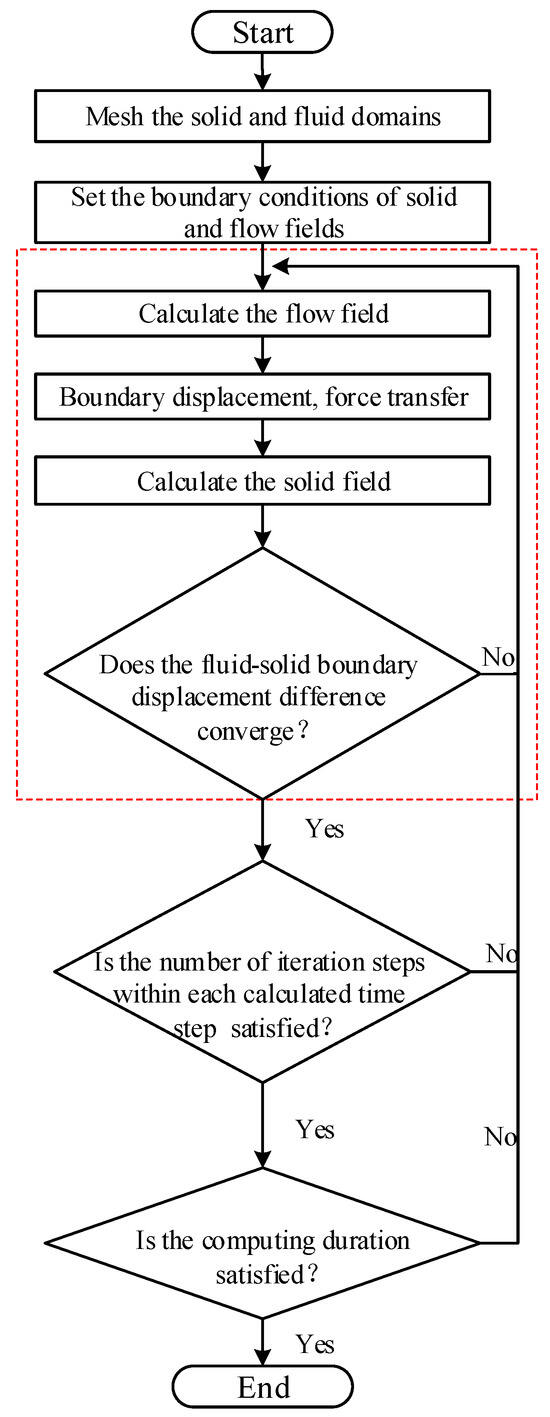
Figure 1.
Calculation flow of fluid–structure interaction.
2.1. Governing Equation of Fluid
The conservation law can be described using the governing equation, where the equation of the conservation of mass is
The equation of the conservation of momentum is
where the subscript is the gas, is the time, is the volume force vector, is the fluid density, is the Laplace operator, is the fluid velocity vector, and is the shear force tensor, which can be expressed as
where is the fluid pressure, is the dynamic viscosity, is the identity matrix, and is the velocity stress tensor, which can be expressed as
2.2. Governing Equation of Solid
The conservation equation of a solid can be derived from Newton’s Second Law of Motion (Force and Acceleration):
where the subscript is the solid, is the density of the solid, is the local acceleration vector in the solid domain, is Cauchy’s stress tensor, and is the volume vector.
2.3. Governing Equation of Energy
The energy conservation equation means that the rate of change of energy in the microelement is equal to the net heat flow into the microelement, the work performed by the volume force and the surface force on the microelement, and the energy conservation equation is
where is the density of the fluid, is the internal energy, is the velocity component, is the temperature, and is the viscous stress tensor.
2.4. Equation of Fluid–Structure Interaction
The fluid–structure interaction must follow the most basic principle of conservation. Therefore, at the fluid–structure interaction interface, the conservation of fluid stress and solid stress (), displacement (), heat flow (), temperature (), and other variables should be met, satisfying the following equations:
3. Numerical Simulation of Mountainous Terrain and Wire
3.1. Model of Mountainous Terrain and Wire
Transmission lines in mountainous terrain are inevitably set up in valleys. An acceleration effect occurs when the wind field passes through the front mountain. The obstruction of the back mountain further complicates the change in the wind field, which has a greater impact on the transmission lines. In this study, an approximately round hammer mountain was selected, and the wire was located between the two mountains. The three-dimensional model of the mountainous terrain and the wire’s route direction are shown in Figure 2, where the direction of the incoming wind is perpendicular to the wire, L is the wire length (L = 60 m), D is the bottom diameter of the mountain (D = 40 m), H is the mountain height (H = 27.5 m), and d is the distance between the bottoms of the two mountains (d = 20 m). The wire is 20 m above the ground.
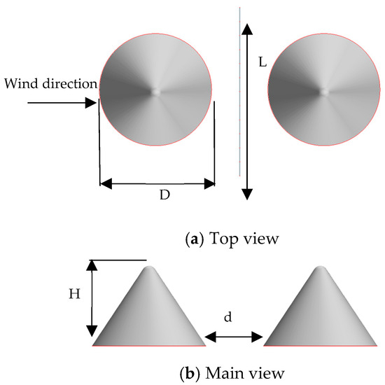
Figure 2.
The three-dimensional model of the mountainous terrain and the wire.
When creating the initial state of the wire, the initial strain and elastic modulus were assigned to the wire, and the load and constraint were applied to obtain the arc sag shape of the wire that met the equilibrium state. The fixed points on both sides of the wire were 20 m high from the ground. The detailed wire parameters are shown in Table 1.

Table 1.
Wire parameters.
3.2. Computing Domain and Grid Division
In this study, the finite element simulation software STAR-CCM+ (2206 Build 17.04.007) [24] was used to establish the numerical simulation model of the traverse in the canyon terrain and perform the fluid–structure interaction calculation. Set the fluid model as Standard Air, the density as 1.29 Kg/m3, and the dynamic viscosity as 1.855 × 10⁻⁵ Pa·s. The calculation domain model and grid division are shown in Figure 3. The overall height of the computing domain was 50 m, the width was 150 m, and the length was 240 m. The fluid region mesh used the cut volume mesh cell generator and the prismatic layer mesh generator. The base mesh size was set to 1 m, the minimum surface size was set to 0.005 m, the maximum mesh cell size was set to 2 m, the number of prismatic layers was set to three, and the total thickness of the prismatic layer was set to 0.01 m.
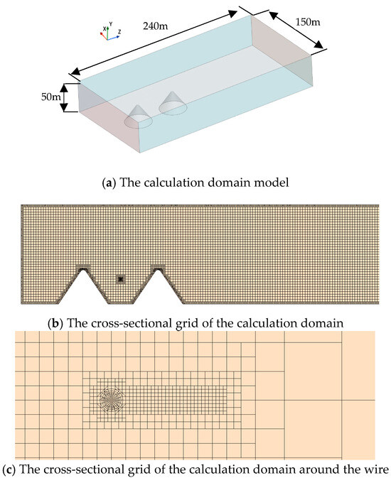
Figure 3.
The calculation domain model and grid division.
The mesh of wire was divided by the block grid of the source surface, using the patch mesh dividing the end face of wire into 85 parts, and the layer number was 120. The grid was locally encrypted in the area around the wire to meet the accuracy of the fluid–structure interaction simulation. The grid division and local amplification of the wire are shown in Figure 4. There were 3.11 million grid cells in the fluid domain, among which there were 10,200 grid cells of wire.
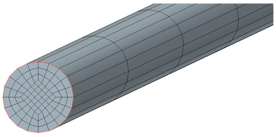
Figure 4.
The grid division of the wire.
3.3. Boundary Conditions and Solutions
The inlet was set as free flow, the wind speed was given via the user function, and the outlet was set as free flow. The side of the flow field was set as a symmetric plane, the bottom surface of the flow field was set as a wall with a non-slip condition, and the top surface of the flow field was set as a wall with a slip condition. The wire surface was set as the fluid–structure interaction interface, which was used to transmit wind pressure and show the structural deformation. The unsteady state was used for the flow field calculation and analysis, the time step was taken as 0.0025 s, and the k-ε turbulence model was used.
3.4. Model Condition
Two inlet wind speeds, the step wind speed (Table 2) and pulse wind speed (Table 3), were set to obtain the vibration characteristics of the transmission lines under different wind field transients. The step wind speed applied to the speed at the inlet, where the speed’s initial value was 2 m/s, and it started to rise at 0.1 s and then stayed the same after reaching the maximum at 1.1 s. Four working conditions were set in total. Under the pulse wind speed condition, the velocity’s initial value was 2 m/s; it started to rise at 0.03 s and reached the maximum at 0.53 s. The maximum velocity was maintained to 1.03 s, and then it decreased to 1.53 s and returned to the initial velocity of 2 m/s, which remained unchanged. Three conditions were set in total.
Table 2.
Step wind speed conditions.
Table 3.
Pulse wind speed conditions.
4. Verification of Accuracy
In order to verify the accuracy of the numerical calculation method used, the problem studied in [25] was selected for calculation and comparison. The wire used in [25] was an ACSR-type wire, with a total outer diameter of 28.62 mm, weight of 1621 kg/km, and rated strength of 131.9 KN. All parameters are similar to those used in this study, so the experimental data in [25] are suitable for verification and comparison with this study. We studied the wind vibration response of a single wire under flat terrain for a uniform flow field. The calculation domain model grid division is shown in Figure 5. The inlet was set as exponent wind speed. Figure 6 shows the comparison between the simulation results of conductor displacement and those in [25]. Under the action of the uniform flow field, the results in this paper agreed well with those in the reference. The accuracy of the numerical calculation method in this paper was verified.
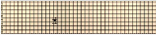
Figure 5.
The cross-sectional grid of the calculation domain.
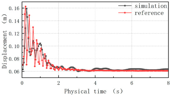
Figure 6.
Comparison of displacement time–history curves.
5. Wind Vibration Characteristics of Wire Under Steady-State Constant Wind Speed Input
A constant wind speed of 20 m/s at the inlet was set for steady state calculation. The flat terrain model was taken as the original condition. The influence of distance between the wire and mountain and mountain size on wind vibration characteristics of the wire are studied.
5.1. Conditions of Different Distances Between Wire and Mountain
The model where a single mountain is located in front of the wire was set and the calculation domain model grid division is shown in Figure 7. The mountain size and position remained the same and the wire position was moved. The working conditions, that the distances between the wire and mountain are 20 m, 30 m, 40 m, and 50 m, were set. The time–history curves of the z-displacement and y-displacement of the midpoint of the wire are shown in Figure 8. Different conditions are expressed in terms of their distances. In the figure legend, the distance is shown as “D”. This can be seen in Figure 8.
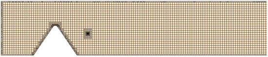
Figure 7.
The cross-sectional grid of the calculation domain.
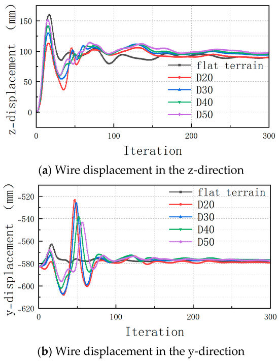
Figure 8.
Time–history curves of displacement.
- (1)
- The distance between the conductor and the mountain mainly affected the vibration of the conductor in the initial stage and it had little effect on the position of the wire’s final stable state. The stable position of the wire at different distances was similar to that of the wire at flat terrain;
- (2)
- The influence of distance on the amplitude of wire vibration displacement was different in different directions. The mountain barrier reduced the lateral force on the wire and the maximum peak value of vibration in the z-direction. The closer the wire was to the mountain, the smaller the maximum peak value of vibration was. The flow past effect caused by the mountain increased the lift force on the wire and the maximum peak value of vibration in the y-direction. The closer the wire was to the mountain, the greater the maximum peak value of vibration was.
5.2. Conditions of Different Mountain Sizes
The model where a single mountain is located in front of the wire was set. The position of the wire and the mountain remained the same. The size of the mountain changed according to the same proportion between the height and the bottom diameter. The conditions of the mountain bottom diameter were set at 30 m, 40 m, 50 m, and 60 m. The time–history curves of the z-displacement and y-displacement of the midpoint of the wire are shown in Figure 9. Different conditions are expressed in terms of their diameters of mountain. In the figure legend, the distance is shown as “DM”. The discussion of different mountain sizes can be converted into the discussion of the proportion of the blocking length of the mountain to the wire total length. After calculation, the blocking ratios of the above conditions were 1.5%, 18.2%, 34.8%, and 51.5%. This can be seen in Figure 9.
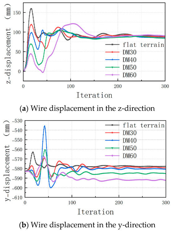
Figure 9.
Time–history curves of displacement.
- (1)
- The displacement of the wire in the z-direction was greatly affected by the blocking ratio in the initial vibration stage. The suppressant effect of the mountain on the wire vibration displacement in the z-direction increased with the increase in the blocking ratio. The final stable state of the wire had little relation with the blocking ratio of the mountain and the stable position of the wire was close to that of the flat terrain;
- (2)
- The vibration peak value of the wire in the y-direction increased first and then decreased with the increase in the blocking ratio. According to the curve in the figure, it can be judged that there will be the maximum peak when the blocking ratio is around 20%. The larger the mountain barrier ratio was, the greater the vertical force in the negative y-direction was on the wire and the lower the final stable position of the wire in the y-direction.
5.3. Condition of Canyon Terrain
The canyon terrain model with the wire located in the middle of two mountains was set, which was the same as the model shown in Figure 3. The time–history curves of the z-displacement and y-displacement of the midpoint of the wire are shown in Figure 10. The figure shows that compared with flat terrain, the displacements of the wire in all directions were similar to that of the single-mountain model. The mountain suppressed the peak vibration in the z-direction and increased the peak vibration in the y-direction.
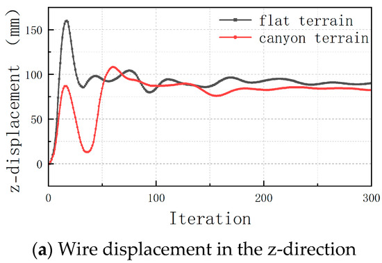
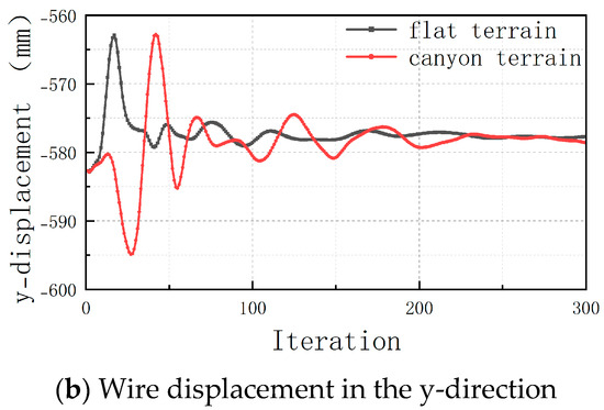
Figure 10.
Time–history curves of displacement.
In summary, the simulation results of the steady-state constant wind speed show that when the transmission line is set up in the mountains and canyon terrain, more emphasis should be placed on avoiding the interference risk of the wire swinging in the vertical direction.
6. Wind Vibration Characteristics of Wire Under Step Wind Speed Input
6.1. Wind Vibration Mechanism of Wire Under Step Wind Speed Input
Figure 11 shows the time–history curves of the inlet wind speed, the pre-line wind speed, the lateral force of the wire, the displacement of the wire in the z-direction, the lift force of the wire, and the displacement of the wire in the y-direction under step condition 2. Figure 12 shows the pressure cloud image around the wire in the central section at different times under condition 2. We selected the time when the wind field started to affect the wire and the time when the wind speed tended to be stable, at which time the pressure changed obviously. This can be seen in Figure 11 and Figure 12.
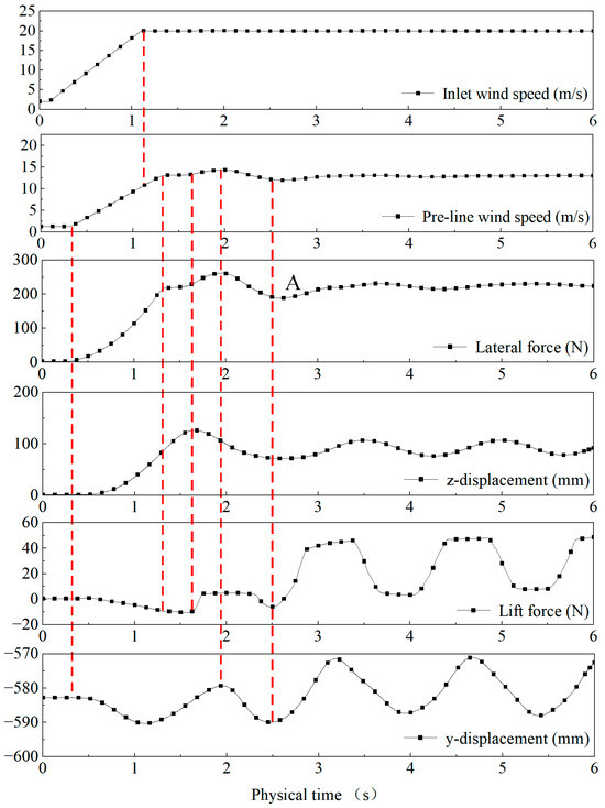
Figure 11.
Time–history curves of wind speed, stress, and wire displacement.
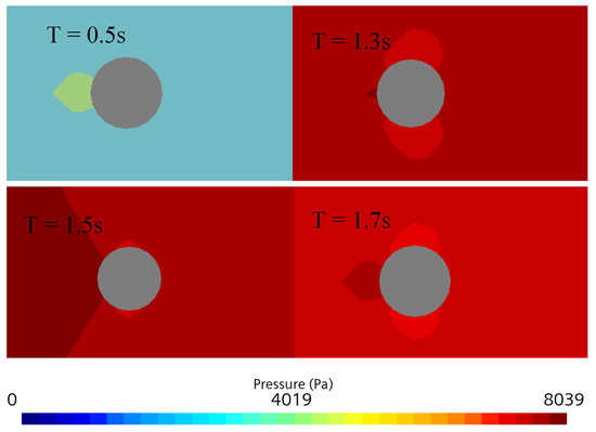
Figure 12.
Pressure around the wire.
- (1)
- The change in air velocity in front of the wire was basically the same as that in the incoming flow. However, affected by the mountain, the peak wind speed around the wire decreased by approximately 40%, and there were obvious local fluctuations;
- (2)
- Lift force and lateral force were generated when the air traversed the wire, and the amplitude of the lateral force was much larger than that of the lift force;
- (3)
- The variation in the lateral force was consistent with the variation in the air velocity in front of the wire. The wire swung under the action of the lateral force;
- (4)
- The lateral force, lift force, y-displacement, and z-displacement entered a periodic decay process and finally re-stabilized after undergoing a transition process under the excitation of the step incoming flow. This transition process ended at the first minimum extreme point of the lateral force (point A in the figure).
6.2. Influence of Different Step Amplitudes
The wind speed change diagram, the lateral force change diagram of the wire, and the time–history curves of the z-displacement and y-displacement of the midpoint of the wire under conditions 1, 2, 3, and 4 are shown in Figure 13. Different conditions are expressed in terms of their accelerations. In the figure legend, the acceleration is shown as “A”. The figure shows that the change trend of the z-direction displacement of the wire was closely related to the lateral force on the wire. Both figures show the wire underwent attenuation oscillation after the wind speed reached stability and eventually reached a stable value. The z-displacement of the wire was analyzed as the step response in the control system. The oscillation attenuation process of the wire was similar to the underdamped step response process of a typical second-order system, with a damping ratio of 0 < ζ < 1. The time domain performance indicators of the control system, calculated from the resulting data for each condition, are shown in Table 4. In the control system, tp is the peak time, and c(tp) is the maximum deviation.
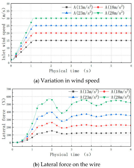
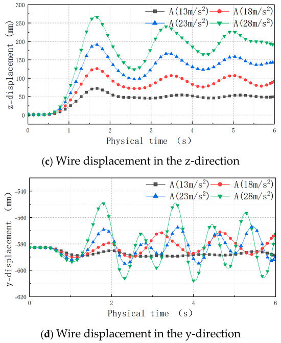
Figure 13.
Time–history curves of wind speed, lateral force, and displacement.
Table 4.
Time domain performance index of each condition (z-direction).
Figure 14 shows the curve of the maximum deviation with the wind speed and the fitted linear trend line. The figure shows that the maximum deviation in the z-direction presented a linear change with the increase in the wind speed. The change equation is
where is the maximum deviation, and is the wind speed.
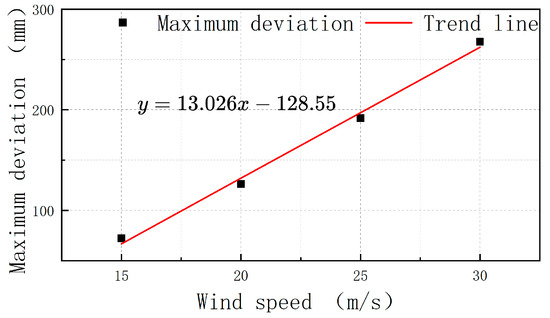
Figure 14.
Change curve and trend line.
Based on the z-direction displacement of the wire, the time required for the wire under each working condition to reach a ±5% error of oscillation within the steady-state value could be obtained, where the adjustment time ts (Δ = 0.05) was successively 6.1 s, 6.4 s, 6 s, and 6.3 s, and the average value was 6.2 s. The variance value of each datum was 0.025, and the degree of data dispersion was small. Therefore, this average value was suitable as the expected value of the adjustment time of each step condition. The peak time of the conductor displacement was close, the overshoot of the conductor displacement was approximately 38.5% (±3%), the oscillation adjustment time was similar, and the displacement oscillation trend was similar. The oscillation period was 1.75 s, 1.82 s, 1.77 s, and 1.74 s in turn, and the average value was 1.77 s. The variance value of each datum was 0.003, and the degree of data dispersion was small. Therefore, this average value was suitable for the expected value of the oscillation period of each step condition. Therefore, the wind vibration response of the wire was mainly determined by its own material characteristics.
The y-displacement diagram of the wire shows that the oscillation amplitude of the conductor in the y-direction increased with the increases in the stable wind speed, and the y-direction oscillation amplitude was smaller than that in the z-direction under every condition.
7. Wind Vibration Characteristics of Wire Under Pulse Wind Speed Input
7.1. Wind Vibration Mechanism of Wire Under Pulse Wind Speed Input
Figure 15 shows the time–history curves of the inlet wind speed, the pre-line wind speed, the lateral force on the wire, the displacement of the wire in the z-direction, the lift force on the wire, and the displacement of the wire in the y-direction under step condition 5. Figure 16 shows the pressure cloud image around the wire in the central section at different times under condition 5. We selected the time of each phase of the change in the pulse wind equally, as seen in Figure 15 and Figure 16.
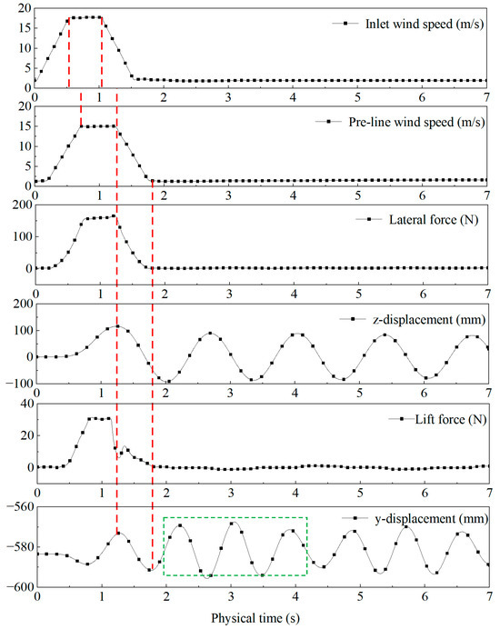
Figure 15.
Time–history curves of wind speed, stress, and wire displacement.
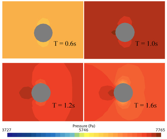
Figure 16.
Pressure around the wire.
- (1)
- Both the lateral force and the z-displacement increased with the rise in the pulse wind and reached the maximum value when the pulse wind started to fall;
- (2)
- After the pulse wind disturbance, the lateral force quickly returned to the pre-disturbance value because the pressure on both sides of the wire was basically equal;
- (3)
- After the pulse wind disturbance, the z-displacement presented periodic fluctuation, and the amplitude gradually decreased;
- (4)
- The lift force increased under the pulse disturbance. However, the vertical direction (y)-displacement continued to fall during this period, which was caused by the combined force of gravity, wire tension, lift, and lateral forces still having a vertical downward component;
- (5)
- A further analysis showed that after the pulse wind disturbance, the y-displacement oscillations underwent a decay process with a group of three wave peaks (the green dashed line in the figure) as the period. The oscillation period of three wave peaks was formed in the y-direction mainly because the positive and negative displacements in the y-direction were not synchronized with those in the z-direction. The positive and negative displacements in the y-direction were opposite to those in the z-direction during the first two wave peaks, and the positive and negative displacements in the third wave peak were the same as those in the z-direction.
Under the pulse wind speed, the midpoint of the wire with the maximum displacement was selected for monitoring. Figure 17 shows the displacement trajectory of the midpoint of the wire under the wind speed of condition 5. The x-direction was perpendicular to the plane of the coordinate axis, and the point corresponding to 0 on the axis in the z-direction was the starting point of the displacement of the midpoint of the wire. The figure shows that the wire swung in the shape of the number “8”. The swing trajectory gradually moved closer to the middle as the swing process progressed, and the stroke trajectory of each cycle gradually decreased. It was predicted that the wire would eventually reach a stable equilibrium state.
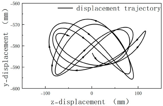
Figure 17.
The midpoint displacement trajectory of the wire.
7.2. Influence of Different Pulse Speed Widths
Figure 18 shows a comparison of the change curves of the pre-line wind speed and midpoint displacement of the wire in the z-direction and y-direction under conditions 5, 6, and 7, respectively. The different conditions are expressed in terms of the speed widths. In the figure legend, the width is shown as “W”.
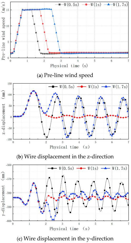
Figure 18.
Time–history curves of pre-line wind speed and displacement.
The figure shows that the influence of turbulence with different pulse widths on the y-direction and z-direction oscillation of the wire was significant. The specific analysis is detailed as follows:
- (1)
- The y-direction displacement under condition 6 was different from that under conditions 5 and 7. After the end of the pulse disturbance, the fluctuation amplitude of the z-direction displacement under condition 6 was much smaller than that under working conditions 5 and 7. That is, the amplitude of the z-direction displacement under condition 6 was significantly larger when the z-direction and lateral force or pulse wind drop were consistent (such as under conditions 5 and 7) than when they were inconsistent (such as under condition 6). Hence, when the pulse wind dropped, the lateral force suppressing the z-direction swing reduced the wind vibration of the wire;
- (2)
- After the end of the pulse disturbance, the amplitude of the y-direction displacement fluctuation under conditions 6 and 7 was much smaller than that under condition 5, which was due to the combined effect of the lateral force and lift force. Moreover, the amplitude of the y-direction oscillation was smaller than that in the z-direction;
- (3)
- Comparing conditions 5 and 7, if the difference in the two pulse widths was an integer multiple of the inherent oscillation period of the wire, then the z-direction oscillation characteristics of the wire were consistent after the pulse disturbance was over;
- (4)
- Comparing conditions 5 and 6, if the difference between the two pulse widths was half of the inherent oscillation period of the wire, then the z-direction oscillation amplitude of the wire was severely suppressed after the pulse disturbance ended.
7.3. Influence of Different Pulse Speed Amplitudes
Figure 19 shows a comparison of the change curves of the pre-line wind speed and the midpoint displacement of the wire in the z-direction and y-direction under conditions 5, 8, and 9, respectively. The different conditions are expressed in terms of their accelerations. In the legend of the figure, acceleration is shown as “A”.
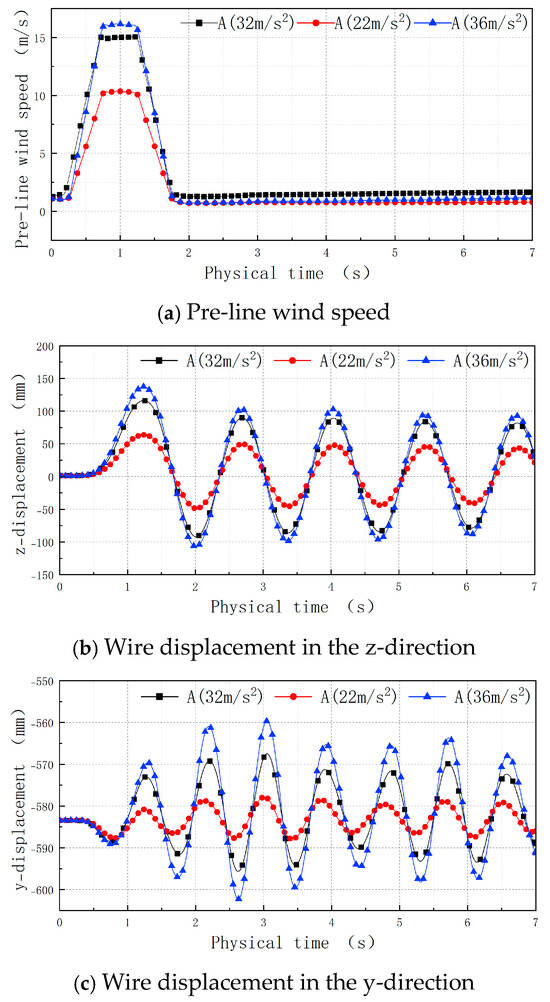
Figure 19.
Time–history curves of pre-line wind speed and displacement.
The maximum wind speeds under conditions 5, 8, and 9 were 18 m/s, 13 m/s, and 20 m/s, respectively. The times of acceleration and deceleration and the maximum wind speed duration of the three conditions were the same. The figure shows that the displacement change situation in the z-direction of the three conditions was the same. After the end of the pulse wind speed, the oscillation attenuation with a single wave peak was carried out in one period, and the change period was the same. The oscillation amplitude increased with the increase in the wind speed amplitude under the different conditions. The displacement change situation in the y-direction of the three conditions was also the same. After the end of the pulse wind speed, the oscillation attenuation was carried out with three peaks as a period, and the oscillation amplitude increased with the increase in the wind speed amplitude under the different working conditions. The maximum swing change amplitude under the three conditions in the z-direction and y-direction is shown in Table 5. The maximum swing amplitude in the y-direction and z-direction increased with the increase in the pulse wind amplitude, but it did so non-linearly.
Table 5.
Maximum amplitude of swing variation.
This analysis demonstrates that the overall law of displacement did not change only when the pulse wind speed amplitude was different, and the main change occurred in the oscillation amplitude.
8. Conclusions
In this study, the distribution characteristics of the wind field and the wind vibration response of the wire under the condition of pulse wind and step wind in the terrain of the double-mountain canyon were examined using numerical simulation software and the strong bidirectional coupling calculation method. The influence of wind field variation on the wind vibration response of the wire was analyzed based on three aspects: the cross-sectional wind field pressure, the wire displacement, and the stress variation. The main conclusions are as follows:
- (1)
- When the wind field reached the wire location after passing through the mountain, the wind speed decreased to a certain extent, and the windward side of the wire always bore the greatest pressure during the whole process of wind speed change. When the wind speed flowing through the wire became uniform, the pressure on the upper part of the wire was the same as that on the lower part of the wire, and the wire depended on inertia and gravity to oscillate;
- (2)
- Under the steady-state constant wind speed, the distance between the conductor and the mountain had little effect on the position of the wire’s final stable state. The mountain size had little effect on the position of the wire’s final stable state in the z-direction and reduced the height in the y-direction. The mountain suppressed the peak vibration in the z-direction and increased the peak vibration in the y-direction;
- (3)
- Under different step wind speed conditions, the displacement change trend of the wire in the inlet wind direction was the same and had a similar oscillation period. Finally, the wire entered a stable state after the same oscillation number. Therefore, the wind vibration response law of the wire was mainly determined by its own material characteristics;
- (4)
- Under the pulse wind speed condition, if the wind speed dropped and the wire swing in the z-direction was inconsistent, the swing amplitude in the z-direction was inhibited. If the difference in the pulse width between the two conditions was an integer multiple of the inherent oscillation period of the wire, the z-direction oscillation characteristics of the wire were consistent after the end of the pulse disturbance. If the difference in the pulse width between the two conditions was half of the inherent oscillation period of the wire, the z-direction swing amplitude of the wire was greatly reduced. The amplitude of the pulse wind did not affect the wire’s oscillation period, and the wire’s oscillation amplitude increased with the increases in the pulse wind amplitude.
According to the wind vibration characteristics of the transmission wires, the wire spacing of some transmission part can be reasonably determined to avoid wind deviation tripping due to the close wire spacing.
There is an important problem to be further studied, which is the problem of breakage of transmission wires under the ice condition by the impact of a wind field. In rainy and snowy weather, the transmission wires will freeze due to low temperature and moisture. In this case, the wire is prone to be overloaded which leads to wire breakage. We will discuss this issue in a future study.
Author Contributions
Conceptualization, J.C. and C.Z.; methodology, C.Z.; software, C.Z.; validation, J.C.; formal analysis, J.C.; investigation, J.C.; resources, J.C.; data curation, J.C.; writing—original draft preparation, J.C.; writing—review and editing, C.Z.; visualization, J.C.; supervision, C.Z.; project administration, C.Z.; funding acquisition, C.Z. All authors have read and agreed to the published version of the manuscript.
Funding
This research was funded by National Natural Science Foundation of China grant number 11762010. And The APC was funded by National Natural Science Foundation of China grant number 11762010.
Institutional Review Board Statement
Not applicable.
Informed Consent Statement
Not applicable.
Data Availability Statement
The original contributions presented in this study are included in the article. Further inquiries can be directed to the corresponding author.
Conflicts of Interest
The authors declare no conflict of interest.
References
- Zhu, Y.K.; Liu, F.J.; Jiang, Z. Micro terrain and microclimate transmission lines of electricity fault analysis and protection measures. Inn. Mong. Electr. Power 2014, 32, 11–14. (In Chinese) [Google Scholar]
- Du, Z.Q.; Xu, Y.H.; Chen, H.; Liu, W.F.; Ma, Y.L.; Chang, B. Study on analysis and prevention methods of wind damage fault in micro terrain region of overhead transmission line. Electrotech. Electr. 2017, 12, 42–45. (In Chinese) [Google Scholar]
- Di, Y.L.; Cai, Z.L.; Li, L.; Yi, Y.S. Analysis of wind characteristics of wide range transmission line galloping in Bohai Rim. Power Syst. Clean Energy 2021, 37, 121–129. (In Chinese) [Google Scholar]
- Zhou, Z.; Zhang, Z.K.; Zhao, Z.G.; Feng, T.; Li, C.; Li, Y.N. Monitoring of wind deflection angle of suspension insulator string for power lines based on optical fiber sensing. J. Electron. Meas. Instrum. 2020, 34, 81–87. (In Chinese) [Google Scholar]
- Wu, F.P.; Xu, Z.; Liu, Z.G.; Song, Y.; Yang, J. Research on wind-induced vibration of flexible catenary under canyon terrain wind. J. China Railw. Soc. 2021, 43, 47–61. (In Chinese) [Google Scholar]
- Wang, D.H.; Han, S.H.; Huang, G.Q.; Yang, Q.S.; Sun, Q.G.; Yang, J.Y. Parametric analysis for dynamic response of transmission lines under tornado. High Volt. Eng. 2022, 48, 3871–3881. (In Chinese) [Google Scholar]
- Huang, S.J.; He, C.; Huang, T.; Wang, C.Y.; Jiang, L.Q.; Cao, M.G. Study of wind deflection response of sealing network caused by coupled high-speed train slipstream. Zhejiang Electr. Power 2021, 40, 29–37. (In Chinese) [Google Scholar]
- Wang, W.; Zhang, Y.L.; Zhang, D.H.; Wang, D.H.; He, Y.X.; Xiang, Y. Comparative analysis on wind load specifications in China and abroad overhead transmission line. South. Power Syst. Technol. 2023, 17, 117–127, 144. (In Chinese) [Google Scholar]
- Hung, P.V.; Yamaguchi, H.; Isozaki, M.; Gull, J.H. Large amplitude vibrations of long-span transmission lines with bundled conductors in gusty wind. J. Wind Eng. Ind. Aerodyn. 2014, 126, 48–59. [Google Scholar] [CrossRef]
- Lin, W.E.; Savory, E.; McIntyre, R.P.; Vandelaar, C.S.; King, J.P.C. The response of an overhead electrical power transmission line to two types of wind forcing. J. Wind Eng. Ind. Aerodyn. 2012, 100, 58–69. [Google Scholar] [CrossRef]
- Wang, F.; Wang, Y.; Zhou, R.; Chen, C. Experiments on aeolian vibration of large span overhead transmission lines. J. Chongqing Univ. 2018, 41, 42–50. (In Chinese) [Google Scholar]
- Azzi, Z.; Elawady, A.; Irwin, P.; Chowdhury, A.G.; Shdid, C.A. Aeroelastic modeling to investigate the wind-induced response of a multi-span transmission lines system. Wind Struct. 2022, 34, 231–257. [Google Scholar]
- Luo, X.Y.; Nie, M.; Xie, W.P.; Xiao, K. Numerical simulations of wind flow over complex terrain where transmission lines locate. Sci. Technol. Eng. 2019, 19, 172–176. (In Chinese) [Google Scholar]
- Liu, M.L.; Lv, H.K.; Luo, K.; Wang, M.J.; Fan, J.R.; Chi, W. Wind induced response numerical simulation of a transmission tower-line system in real mountainous terrain. J. Vib. Shock 2020, 39, 232–239. (In Chinese) [Google Scholar]
- Deng, Y.; Jiang, X.L.; Wang, H.X.; Yang, Y.; Virk, M.S.; Liao, Y.; Wu, J.G.; Zhao, M.G. Multimodal analysis of saddle micro-terrain prone to wind disasters on overhead transmission lines. Electr. Power Syst. Res. 2024, 229, 110143. [Google Scholar]
- Lou, W.J.; Wu, D.G.; Liu, M.M.; Zhang, L.G.; Bian, R. Properties of mountainous terrain wind field and their influence on wind-induced swing of transmission lines. China Civ. Eng. J. 2018, 51, 46–55, 77. (In Chinese) [Google Scholar]
- Zhong, W.J.; Yao, J.F.; Tu, Z.B.; Xu, H.W. Wind induced coupling effects of transmission tower-line system at microtopography. J. Phys. Conf. Ser. 2023, 2592, 012093. [Google Scholar] [CrossRef]
- Reinoso, E.; Nino, M.; Berny, E.; Inzunza, I. Wind Risk Assessment of Electric Power Lines due to Hurricane Hazard. Nat. Hazards Rev. 2020, 21, 04020010. [Google Scholar]
- Yang, S.; Chouinard, L.E.; Langlois, S. Hourly wind data for aeolian vibration analysis of overhead transmission line conductors. J. Wind Eng. Ind. Aerodyn. 2022, 230, 105184. [Google Scholar]
- Wu, C.; Yang, X.H.; Zhang, B.; Liu, Z.H.; Zhao, Y. Dynamic Response of a Cat Head Type Transmission Tower-line System under Strong Wind. J. Phys. Conf. Ser. 2021, 1986, 012098. [Google Scholar] [CrossRef]
- Kim, J.W.; Sohn, J.H. Galloping Simulation of the Power Transmission Line under the Fluctuating Wind. Int. J. Precis. Eng. Manuf. 2018, 19, 1393–1398. [Google Scholar]
- Dikshit, S.; Dobson, I.; Alipour, A. Cascading structural failures of towers in an electric power transmission line due to straight line winds. Reliab. Eng. Syst. Saf. 2024, 250, 110304. [Google Scholar]
- Chen, B.; Liu, R.G.; Xie, G.H. Numerical Simulation and Test on Wind-induced Transient Dynamic Response of CFRP Cable. China J. Highw. Transp. 2015, 28, 54–61. (In Chinese) [Google Scholar]
- Jin, Y.; Chen, X. Using STAR-CCM+ Software in Aerodynamic Performance of Bogies under Crosswind Conditions. EAI Endorsed Trans. Energy Web 2024, 11, 1–12. [Google Scholar]
- Riera, J.D.; Oliveira, T.T. Wind-structure interaction in conductor bundles in transmission lines. Struct. Infrastruct. Eng. 2010, 6, 435–446. [Google Scholar]
Disclaimer/Publisher’s Note: The statements, opinions and data contained in all publications are solely those of the individual author(s) and contributor(s) and not of MDPI and/or the editor(s). MDPI and/or the editor(s) disclaim responsibility for any injury to people or property resulting from any ideas, methods, instructions or products referred to in the content. |
© 2025 by the authors. Licensee MDPI, Basel, Switzerland. This article is an open access article distributed under the terms and conditions of the Creative Commons Attribution (CC BY) license (https://creativecommons.org/licenses/by/4.0/).