
DualCascadeTSF-MobileNetV2: A Lightweight Violence Behavior Recognition Model


Abstract
1. Introduction
- 1.
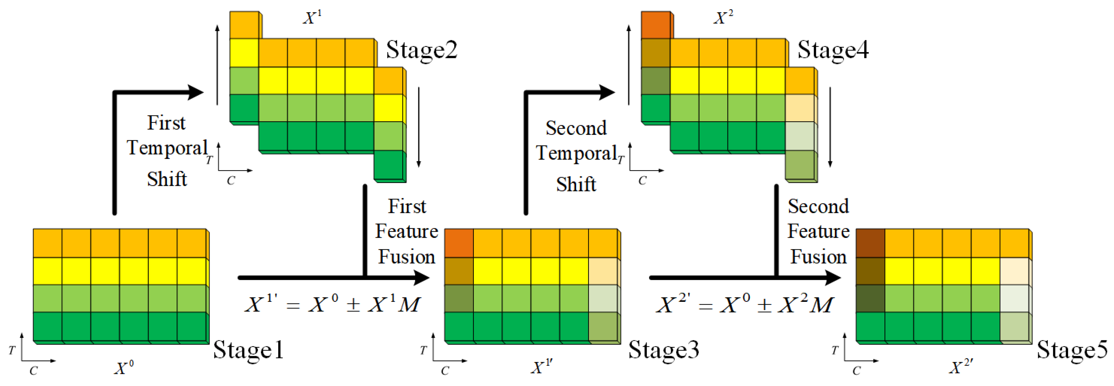
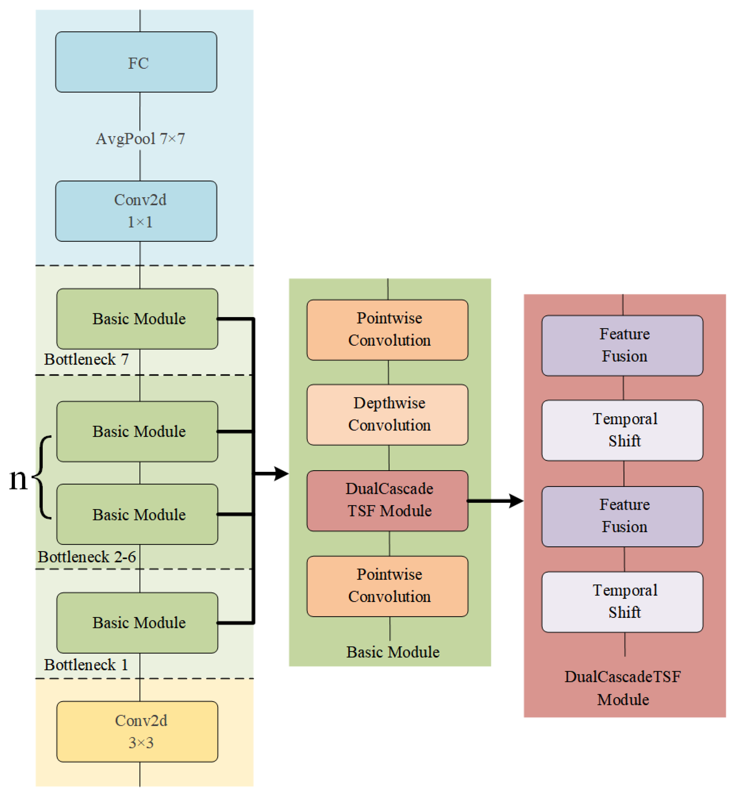
- Improved TSM based on previous studies and designed the Dual Cascade Temporal Shift and Fusion (DualCascadeTSF) module. This module cascades two temporal shift modules and enhances the model’s ability to extract long-term temporal information by adding feature fusion [2] after each temporal shift. It improves the robustness and accuracy of the model without increasing additional parameters.
- 2.
- Combined the DualCascadeTSF module with the MobileNetV2. This not only improves the accuracy of MobileNetV2, but also makes it have fewer parameters and a faster operation speed compared to other classic models, making it more suitable for deployment on edge devices.
2. Related Work
2.1. Research on Lightweight Models
2.2. TSM and Two-Cascade TSM
2.3. MobileNetV2
3. Methods
3.1. Conception
3.2. DualCascadeTSF Module
3.3. DualCascadeTSF-MobileNetV2
4. Experiments
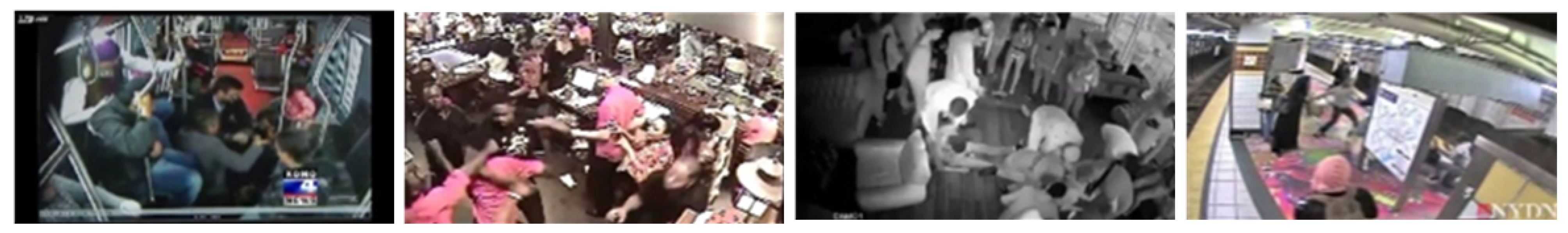
4.1. Datasets
4.2. Parameter Settings
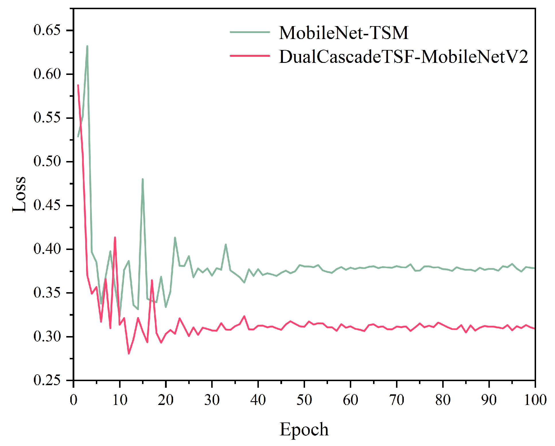
4.3. Results
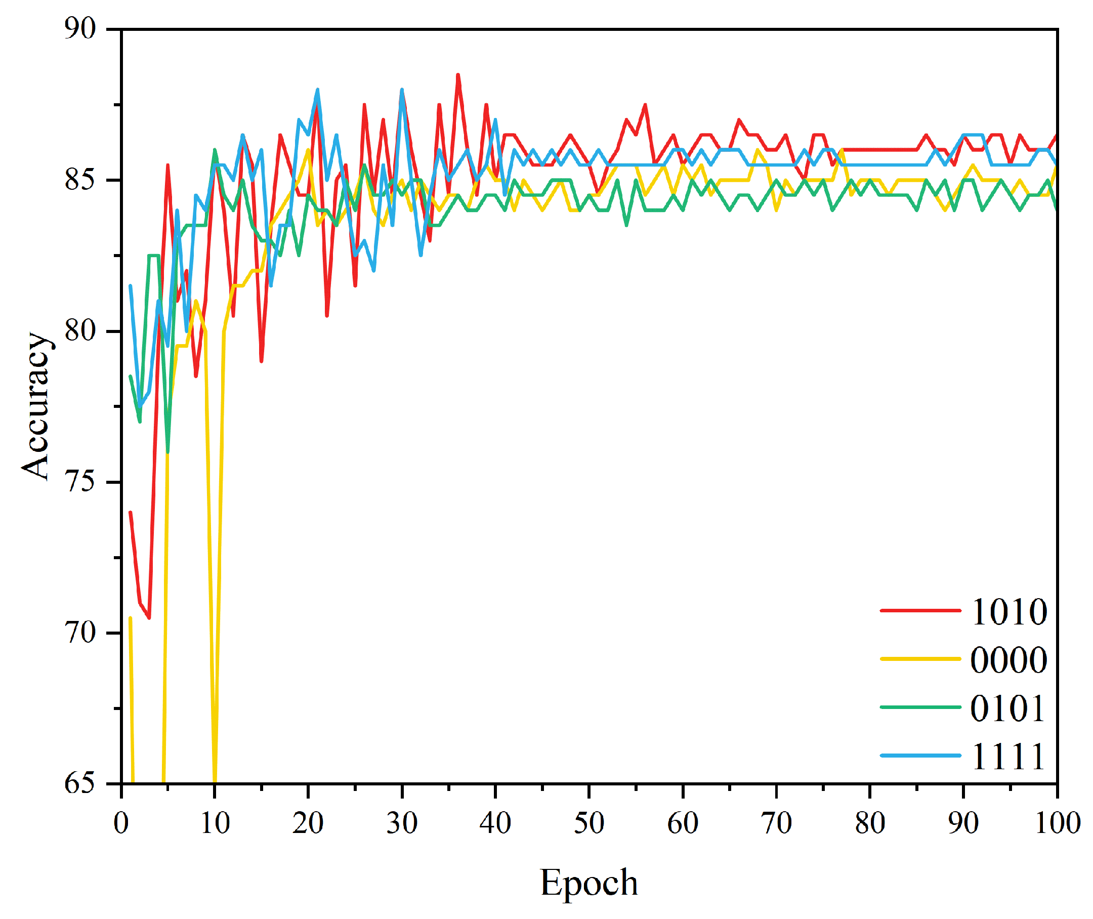
4.3.1. Ablation Experiments of Different Feature Fusion Methods
4.3.2. Ablation Study on Different Structures
4.3.3. Comparative Experiments with Classic Models
5. Discussion
6. Conclusions
Author Contributions
Funding
Institutional Review Board Statement
Informed Consent Statement
Data Availability Statement
Conflicts of Interest
Abbreviations
| DualCascadeTSF | Dual Cascade Temporal Shift and Fusion module |
| TSM | temporal shift module |
References
- Lin, J.; Gan, C.; Han, S. TSM: Temporal Shift Module for Efficient Video Understanding. In Proceedings of the 2019 IEEE/CVF International Conference on Computer Vision (ICCV), Seoul, Republic of Korea, 27 October–5 November 2019. [Google Scholar]
- Lian, Z.; Yin, Y.; Lu, J.; Xu, Q.; Zhi, M.; Hu, W.; Duan, W. A Survey: Feature Fusion Method for Object Detection Field. In Advanced Intelligent Computing Technology and Applications; Springer Nature: Singapore, 2024. [Google Scholar]
- Liu, Z.; Li, J.; Shen, Z.; Huang, G.; Yan, S.; Zhang, C. Learning Efficient Convolutional Networks through Network Slimming. In Proceedings of the 2017 IEEE International Conference on Computer Vision (ICCV), Venice, Italy, 22–29 October 2017. [Google Scholar]
- Li, H.; Kadav, A.; Durdanovic, I.; Samet, H.; Graf, M.P. Pruning Filters for Efficient ConvNets. arXiv 2016, arXiv:1608.08710. [Google Scholar]
- Sanh, V.; Wolf, T.; Rush, A.M. Movement Pruning: Adaptive Sparsity by Fine-Tuning. arXiv 2020, arXiv:2005.07683. [Google Scholar]
- Howard, A.G.; Zhu, M.; Chen, B.; Kalenichenko, D.; Wang, W.; Wey, T.; Andreetto, M.; Adam, H. MobileNets: Efficient Convolutional Neural Networks for Mobile Vision Applications. arXiv 2017, arXiv:1704.04861. [Google Scholar]
- Sandler, M.; Howard, A.; Zhu, M.; Zhmoginov, A.; Chen, L.-C. MobileNetV2: Inverted Residuals and Linear Bottlenecks. In Proceedings of the 2018 IEEE/CVF Conference on Computer Vision and Pattern Recognition, Salt Lake City, UT, USA, 18–23 June 2018. [Google Scholar]
- Zhang, X.; Zhou, X.; Lin, M.; Sun, J. ShuffleNet: An Extremely Efficient Convolutional Neural Network for Mobile Devices. In Proceedings of the 2018 IEEE/CVF Conference on Computer Vision and Pattern Recognition, Salt Lake City, UT, USA, 18–23 June 2018. [Google Scholar]
- Iandola, F.N.; Han, S.; Moskewicz, M.W.; Ashraf, K.; Dally, W.J.; Keutzer, K. SqueezeNet: AlexNet-level accuracy with 50x fewer parameters and <0.5MB model size. arXiv 2016, arXiv:1602.07360. [Google Scholar]
- Howard, A.; Sandler, M.; Chen, B.; Wang, W.; Chen, L.-C.; Tan, M.; Chu, G.; Vasudevan, V.; Zhu, Y.; Pang, R.; et al. Searching for MobileNetV3. In Proceedings of the 2019 IEEE/CVF International Conference on Computer Vision (ICCV), Seoul, Republic of Korea, 27 October–2 November 2019. [Google Scholar]
- Tan, M.; Le, Q.V. EfficientNet: Rethinking Model Scaling for Convolutional Neural Networks. In Proceedings of the 36th International Conference on Machine Learning, Long Beach, CA, USA, 10–15 June 2019; Volume 2. [Google Scholar]
- Wang, X.; Xiang, T.; Zhang, C.; Song, Y.; Liu, D.; Huang, H.; Cai, W. BiX-NAS: Searching Efficient Bi-directional Architecture for Medical Image Segmentation. In Medical Image Computing and Computer Assisted Intervention–MICCAI 2021, Proceedings of the 24th International Conference, Strasbourg, France, 27 September–1 October 2021, Proceedings, Part I 24; Springer International Publishing: Cham, Switzerland, 2021; pp. 229–238. [Google Scholar]
- Yan, B.; Peng, H.; Wu, K.; Wang, D.; Fu, J.; Lu, H. LightTrack: Finding Lightweight Neural Networks for Object Tracking via One-Shot Architecture Search. In Proceedings of the 2021 IEEE/CVF Conference on Computer Vision and Pattern Recognition (CVPR), Nashville, TN, USA, 20–25 June 2021. [Google Scholar]
- Cai, H.; Gan, C.; Han, S. Once for All: Train One Network and Specialize it for Efficient Deployment. arXiv 2019, arXiv:1908.09791. [Google Scholar]
- Liang, Q.; Li, Y.; Chen, B.; Yang, K. Violence behavior recognition of two-cascade temporal shift module with attention mechanism. J. Electron. Imaging 2021, 30, 43009. [Google Scholar] [CrossRef]
- Gholami, A.; Kwon, K.; Wu, B.; Tai, Z.; Yue, X.; Jin, P.; Zhao, S.; Keutzer, K. SqueezeNext: Hardware-Aware Neural Network Design. In Proceedings of the 2018 IEEE/CVF Conference on Computer Vision and Pattern Recognition Workshops (CVPRW), Salt Lake City, UT, USA, 18–22 June 2018. [Google Scholar]
- Wu, B.; Wan, A.; Yue, X.; Keutzer, K. Shift: A Zero FLOP, Zero Parameter Alternative to Spatial Convolutions. In Proceedings of the IEEE Computer Society Conference on Computer Vision and Pattern Recognition, Salt Lake City, UT, USA, 18–22 June 2018; pp. 9127–9135. [Google Scholar]
- Qin, D.; Leichner, C.; Delakis, M.; Fornoni, M.; Luo, S.; Yang, F.; Wang, W.; Banbury, C.; Ye, C.; Akin, B.; et al. MobileNetV4: Universal Models for the Mobile Ecosystem. In Computer Vision—ECCV 2024, Proceedings of the 18th European Conference, Milan, Italy, 29 September–4 October 2024, Proceedings, Part XL; Springer: Cham, Switzerland, 2024. [Google Scholar]
- Tan, M.; Le, Q.V. EfficientNetV2: Smaller Models and Faster Training. In Proceedings of the 38th International Conference on Machine Learning, Baltimore, MD, USA, 17–23 July 2022. [Google Scholar]
- Wang, A.; Chen, H.; Lin, Z.; Han, J.; Ding, G. Rep ViT: Revisiting Mobile CNN From ViT Perspective. In Proceedings of the 2024 IEEE/CVF Conference on Computer Vision and Pattern Recognition (CVPR), Seattle, WA, USA, 16–22 June 2024. [Google Scholar]
- Han, K.; Wang, Y.; Tian, Q.; Guo, J.; Xu, C.; Xu, C. GhostNet: More Features From Cheap Operations. In Proceedings of the 2020 IEEE/CVF Conference on Computer Vision and Pattern Recognition (CVPR), Seattle, WA, USA, 14–19 June 2020. [Google Scholar]
- Tang, Y.; Han, K.; Guo, J. GhostNetV2: Enhance Cheap Operation with Long-Range Attention. In Proceedings of the Advances in Neural Information Processing Systems 35 (NeurIPS 2022), New Orleans, LA, USA, 28 November–9 December 2022. [Google Scholar]
- Han, K.; Wang, Y.; Xu, C.; Guo, J.; Xu, C.; Wu, E.; Tian, Q. GhostNets on Heterogeneous Devices via Cheap Operations. Int. J. Comput. Vis. 2022, 130, 1050–1069. [Google Scholar] [CrossRef]
- Ma, N.; Zhang, X.; Zheng, H.-T.; Sun, J. ShuffleNet V2: Practical Guidelines for Efficient CNN Architecture Design. In Proceedings of the Computer Vision, 15th European Conference (ECCV 2018), Munich, Germany, 8–14 September 2018. [Google Scholar]
- Freeman, I.; Roese-Koerner, L.; Kummert, A. EffNet: An Efficient Structure for Convolutional Neural Networks. In Proceedings of the 2018 25th IEEE International Conference on Image Processing (ICIP), Athens, Greece, 7–10 October 2018. [Google Scholar]
- Hassner, T.; Itcher, Y.; Kliper-Gross, O. Violent flows: Real-time detection of violent crowd behavior. In Proceedings of the 2012 IEEE Computer Society Conference on Computer Vision and Pattern Recognition Workshops, Providence, RI, USA, 16–21 June 2012. [Google Scholar]
- Cheng, M.; Cai, K.; Li, M. RWF-2000: An Open Large Scale Video Database for Violence Detection. In Proceedings of the 2020 25th International Conference on Pattern Recognition (ICPR), Milan, Italy, 10–15 January 2021. [Google Scholar]
- Bermejo Nievas, E.; Deniz Suarez, O.; Bueno Garcia, G.; Sukthankar, R. Violence Detection in Video Using Computer Vision Techniques. In Proceedings of the International Conference on Computer Analysis of Images and Patterns, Seville, Spain, 29–31 August 2011. [Google Scholar]
- Zhang, Y.; Li, Y.; Guo, S. Lightweight mobile network for real-time violence recognition. PLoS ONE 2022, 17, e0276939. [Google Scholar]
- Shafiq, M.; Gu, Z. Deep Residual Learning for Image Recognition: A Survey. Appl. Sci. 2022, 12, 8972. [Google Scholar] [CrossRef]
- Ji, S.; Xu, W.; Yang, M.; Yu, K. 3D convolutional neural networks for human action recognition. IEEE Trans. Pattern Anal. Mach. Intell. 2013, 35, 221–231. [Google Scholar] [PubMed]
- Donahue, J.; Hendricks, L.A.; Rohrbach, M.; Venugopalan, S.; Guadarrama, S.; Saenko, K.; Darrell, T. Long-Term Recurrent Convolutional Networks for Visual Recognition and Description. IEEE Trans. Pattern Anal. Mach. Intell. 2017, 39, 677–691. [Google Scholar] [CrossRef] [PubMed]
- Carreira, J.; Zisserman, A. Quo Vadis, action recognition? A new model and the kinetics dataset. In Proceedings of the 2017 IEEE Conference on Computer Vision and Pattern Recognition (CVPR), Honolulu, HI, USA, 22–25 July 2017. [Google Scholar]
- Wang, W.; Dong, S.; Zou, K.; Li, W. A Lightweight Network for Violence Detection. In Proceedings of the ICIGP 2022: 2022 the 5th International Conference on Image and Graphics Processing (ICIGP), Beijing, China, 7–9 January 2022. [Google Scholar]
- Meng, Y.; Lin, C.-C.; Panda, R.; Sattigeri, P.; Karlinsky, L.; Oliva, A.; Saenko, K.; Feris, R. AR-Net: Adaptive Frame Resolution for Efficient Action Recognition. In Computer Vision–ECCV 2020, Proceedings of the16th European Conference, Glasgow, UK, 23–28 August 2020, Proceedings, Part VII 16; Springer: Cham, Switzerland, 2020. [Google Scholar]
- Li, Y.; Ji, B.; Shi, X.; Zhang, J.; Kang, B.; Wang, L. TEA: Temporal Excitation and Aggregation for Action Recognition. In Proceedings of the 2020 IEEE/CVF Conference on Computer Vision and Pattern Recognition (CVPR), Seattle, WA, USA, 14–19 June 2020. [Google Scholar]
- Asad, M.; Jiang, H.; Yang, J.; Tu, E.; Malik, A.A. Multi-Level Two-Stream Fusion-Based Spatio-Temporal Attention Model for Violence Detection and Localization. Int. J. Pattern Recognit. Artif. Intell. 2022, 36, 2255002. [Google Scholar]
- Mohammadi, H.; Nazerfard, E. Video violence recognition and localization using a semi-supervised hard attention model. Expert Syst. Appl. 2023, 212, 118791. [Google Scholar]
- Zhang, Y.; Li, Y.; Guo, S.; Liang, Q. Not all temporal shift modules are profitable. J. Electron. Imaging 2022, 31, 043030. [Google Scholar]
- Wang, L.; Xiong, Y.; Wang, Z.; Qiao, Y.; Lin, D.; Tang, X.; Van Gool, L. Temporal Segment Networks: Towards Good Practices for Deep Action Recognition. In Computer Vision—ECCV 2016, Proceedings of the 14th European Conference, Amsterdam, The Netherlands, 11–14 October 2016, Proceedings, Part VIII; Springer: Cham, Switzerland, 2016; Volume 9912, pp. 20–36. [Google Scholar]


| Model | Weights | Computational Complexity | Top-1 Acc. | Top-5 Acc. | Dataset |
|---|---|---|---|---|---|
| SqueezeNet_8bit [9] | 0.66 | — | 57.5 | 80.3 | ImageNet |
| 1.0_SqueezeNext_23 [16] | 0.72 | 282M MAC | 58.98 | 82.33 | ImageNet |
| ShiftNet_A [17] | 4.1 | — | 70.1 | — | ImageNet |
| MobileNet_1 [6] | 4.2 | 569M Mult-Add | 70.6 | — | ImageNet |
| MobileNetV2_1 [7] | 3.4 | 300M Mult-Add | 72.0 | — | ImageNet |
| MobileNetV3_Large_1 [10] | 4.0 | 155M Mult-Add | 73.3 | — | ImageNet |
| MobileNetV4_Conv_M [18] | 9.2 | 1.0G MAC | 79.9 | — | ImageNet |
| EfficientNet_B0 [11] | 5.3 | 0.39B FLOP | 77.1 | 93.3 | ImageNet |
| EfficientNetV2_M [19] | 54 | 24B FLOP | 85.1 | — | ImageNet |
| RepViT_M1.0 [20] | 6.8 | 1.1G MAC | 80.0 | — | ImageNet |
| GhostNet_1 [21] | 5.2 | 141M FLOP | 73.9 | 91.4 | ImageNet |
| GhostNetV2_1.0 [22] | 6.1 | 167M FLOP | 75.3 | 92.4 | ImageNet |
| C_GhostNet_1 [23] | 5.2 | 141M FLOP | 73.9 | 91.4 | ImageNet |
| G_GhostNet_w/_mix [23] | 14.6 | 2.3B FLOP | 73.1 | 91.2 | ImageNet |
| ShuffleNet_1(g=8) [8] | — | 140M FLOP | 67.6 | — | ImageNet |
| ShuffleNetV2_1 [24] | — | 146M FLOP | 69.4 | — | ImageNet |
| EffNet [25] | 0.14 | 11.4M FLOP | 80.20 | — | CIFAR-10 |
| Layer | Structure | DualCascadeTSF Included | Output Size | Repetition Times |
|---|---|---|---|---|
| conv1 | 3 × 3 × 32 | 112 × 112 | ×1 | |
| bottleneck1 | 1 × 1 × 32, 3 × 3 × 32, 1 × 1 × 16 | Yes | 112 × 112 | ×1 |
| bottleneck2 | 1 × 1 × 96, 3 × 3 × 96, 1 × 1 × 24 | Yes | 56 × 56 | ×2 |
| bottleneck3 | 1 × 1 × 192, 3 × 3 × 192, 1 × 1 × 32 | Yes | 28 × 28 | ×3 |
| bottleneck4 | 1 × 1 × 384, 3 × 3 × 384, 1 × 1 × 64 | Yes | 14 × 14 | ×4 |
| bottleneck5 | 1 × 1 × 576, 3 × 3 × 576, 1 × 1 × 96 | Yes | 14 × 14 | ×3 |
| bottleneck6 | 1 × 1 × 960, 3 × 3 × 960, 1 × 1 × 160 | Yes | 7 × 7 | ×3 |
| bottleneck7 | 1 × 1 × 960, 3 × 3 × 960, 1 × 1 × 320 | Yes | 7 × 7 | ×1 |
| conv2 | 1 × 1 × 1280 | 7 × 7 | ×1 | |
| Avgpool | Pool 7 × 7 | 1 × 1 | ×1 | |
| FC | Linear 1280 → 2 | 1 × 1 | ×1 |
| Model | Crowd Violence (%) | RWF-2000 (%) | Hockey Fights (%) |
|---|---|---|---|
| ResNet-50 [30] | 93.878 | 84 | 95.5 |
| 3D-CNN [31] | 94.3 | 82.75 | 94.4 |
| LRCN [32] | 94.57 | 77 | 97.1 |
| I3D [33] | 88.89 | 85.75 | 97.5 |
| MiNet-3D [34] | 91.41 | 81.98 | 94.71 |
| AR-Net [35] | 95.918 | 87.3 | 97.2 |
| TSM [1] | 95.95 | 88 | 97.5 |
| TEA [36] | 96.939 | 88.5 | 97.7 |
| Two-cascade TSM [15] | 96.939 | 89 | 98.05 |
| SAM [37] | 98.15 | 89.1 | 99.1 |
| SSHA [38] | - | 90.4 | 98.7 |
| P-TSM [39] | 96.969 | 91 | 98.5 |
| MobileNet-TSM [29] | 97.959 | 87.75 | 97.5 |
| DualCascadeTSM-MobileNetV2 (ours) | 98.98 | 88.5 | 98.0 |
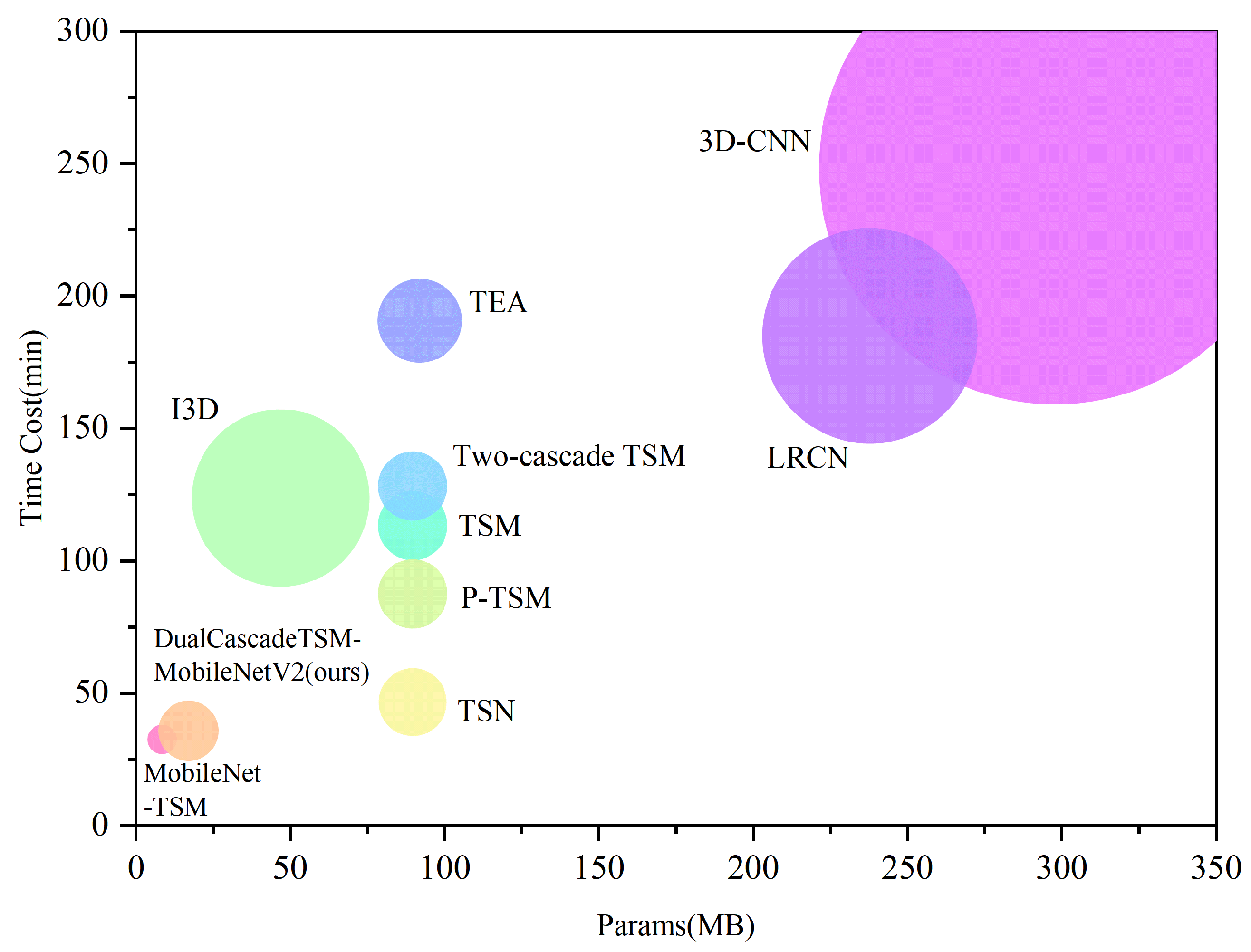
| Model | Parameters (MB) | Training Speed (min) | Memory Size (MB) | GFLOPs |
|---|---|---|---|---|
| 3D-CNN [31] | 297.83 | 248.38 | 2647.7 | 191.6 |
| LRCN [32] | 237.83 | 185.12 | 1212.93 | 186.0 |
| I3D [33] | 46.88 | 123.8 | 1000.2 | 35.6 |
| TSN [40] | 89.69 | 46.68 | 390.05 | 125.3 |
| TSM [1] | 89.69 | 113.43 | 397.71 | 68.1 |
| TEA [36] | 91.95 | 190.8 | 479.78 | 69.9 |
| Two-cascade TSM [15] | 89.69 | 128.33 | 397.71 | 68.1 |
| P-TSM [39] | 89.69 | 87.63 | 396.57 | 68.1 |
| MobileNet-TSM [29] | 8.49 | 32.68 | 175.86 | 5.0 |
| DualCascadeTSM-MobileNetV2 (ours) | 16.99 | 35.92 | 347.13 | 5.0 |
Disclaimer/Publisher’s Note: The statements, opinions and data contained in all publications are solely those of the individual author(s) and contributor(s) and not of MDPI and/or the editor(s). MDPI and/or the editor(s) disclaim responsibility for any injury to people or property resulting from any ideas, methods, instructions or products referred to in the content. |
© 2025 by the authors. Licensee MDPI, Basel, Switzerland. This article is an open access article distributed under the terms and conditions of the Creative Commons Attribution (CC BY) license (https://creativecommons.org/licenses/by/4.0/).
Share and Cite
Chen, Y.; Li, Y.; Li, S.; Lv, S.; Lin, F. DualCascadeTSF-MobileNetV2: A Lightweight Violence Behavior Recognition Model. Appl. Sci. 2025, 15, 3862. https://doi.org/10.3390/app15073862
Chen Y, Li Y, Li S, Lv S, Lin F. DualCascadeTSF-MobileNetV2: A Lightweight Violence Behavior Recognition Model. Applied Sciences. 2025; 15(7):3862. https://doi.org/10.3390/app15073862
Chicago/Turabian StyleChen, Yuang, Yong Li, Shaohua Li, Shuhan Lv, and Fang Lin. 2025. "DualCascadeTSF-MobileNetV2: A Lightweight Violence Behavior Recognition Model" Applied Sciences 15, no. 7: 3862. https://doi.org/10.3390/app15073862
APA StyleChen, Y., Li, Y., Li, S., Lv, S., & Lin, F. (2025). DualCascadeTSF-MobileNetV2: A Lightweight Violence Behavior Recognition Model. Applied Sciences, 15(7), 3862. https://doi.org/10.3390/app15073862