Computational Strategy for Analyzing Effective Properties of Random Composites—Part I: Conductivity

Abstract

The notion of “randomness” in the mathematical theory of composites has typically been used abstractly within measure theory, making practical applications difficult. In contrast, engineering sciences often discuss randomness too loosely, lacking a theoretical foundation. This paper aims to bridge the gap between theory and applications, focusing on the effective properties of two-dimensional conducting composites with non-overlapping circular inclusions. It is shown that there is no universal minimum number of inclusions per cell in simulations of random composites. Even minor changes to Random Sequential Addition algorithms lead to different formulas for the effective constants. Application of the analytical representative volume element (aRVE) theory methodologically and practically addresses the diversity issue of random composites based on homogenization principles. In particular, it examines how the spatial arrangement of inclusions impacts the overall composite properties. The proposed method can be applied to a large number of inclusions and to symbolically given geometric and physical parameters relevant to optimal design problems. The method leverages structural sums and enables a more refined classification of different classes of composites, which was unattainable using previous approaches. The obtained results demonstrate a diversity of apparently similar composites. This paper outlines the investigation strategy and provides a detailed description of each step.

1. Introduction

Random media is a popular topic in modern material science and physics. In this paper, we focus on stationary two-dimensional processes in dispersed composites and discuss their effective properties within the framework of constructive homogenization theory.

To illustrate the central concept of random media, we consider steady heat conduction. This formalism can also be applied to electric, magnetic, dielectric, diffusion, and other processes governed by Laplace’s equation. Furthermore, the same homogenization concept could be extended to elasticity, piezoelectricity, and viscous fluids. These subjects will be discussed in a separate paper.

The effective properties of random composite materials can be estimated on the basis of the representative volume element (RVE). Hill [1] introduced the theoretical principles of RVE as “… a sample that (a) is structurally entirely typical of the entire mixture on average, and (b) contains a sufficient number of inclusions for the apparent overall moduli to be effectively independent of the surface values of traction and displacement”. Hill’s principles are frequently considered as a definition of RVE. Usually, numerical computations of effective constants are supported by a statistical approach when random inclusions are selected within a cell, and the effective constants are calculated based on the numerically given properties of constituents; see [2,3,4,5] and the works cited there. Authors typically imply, though do not explicitly state, that they consider a solely uniform, non-overlapping distribution. Sometimes, the manipulations employed along the way are not grounded in homogenization theory. Sometimes, random locations may not be accurately simulated by computational rules [6] similar to those used in pseudo-random number simulations. This naive statistical approach is prevalent in the engineering literature concerning random composites.

This situation must be rectified according to the mathematical principles established in homogenization theory [7,8,9]. The rules of asymptotic analysis [10,11,12,13] and the upper and lower bounds should be obeyed [14,15]. This paper aims to bridge the gap between rigorous mathematical theory and simplified engineering formulas for effective constants. It presents a strategy for studying random composites based on Image Analysis, partial differential equations (PDEs), computational simulations, and statistical processing.

It should be noted that homogenization theory justifies the existence of effective constants under certain natural conditions and identifies the boundary value problem that must be solved to determine them. The existence and uniqueness of the solution to such a problem are essential results of the mathematical problems addressed. Then, the effective conductivity tensor ${\mathit{\lambda }}_e$ should be computed. The effective tensors can be derived from a periodic boundary value problem with N inclusions per periodicity cell Q, representing the composite under consideration displayed in Figure 1.

The process of generating random arrangements of N inclusions within a two-dimensional domain Q gives examples of a microstructure. Two well-established approaches, such as random walks (RW) and Random Sequential Addition (RSA), are frequently employed to achieve this goal. Each method has well-defined procedural characteristics emergent from specific scenarios for randomness generation.

Various mathematical methods are applied to samples with microstructure to determine the effective properties of random composites. These methods can be divided into three types: pure numerical, e.g., the Finite Element Method (FEM), empirical formulas, and analytical techniques. These methods will be discussed in the following subsections.

1.1. FEM

The FEM is effective for deterministic composite materials when the geometry is defined precisely. In the latter case of composites, the physical (mechanical) properties of the constituents are given numerically [16,17,18,19]. One can use a standard package for a few inclusions to determine the local fields and compute the effective constants by averaging over Q. However, the FEM can not be properly extended to dispersed random composites since the statistical processing of computational experiments is lacking. The typical strategy for random composite materials analysis using the FEM is as follows. Firstly, one has to consider a few numerical examples with few inclusions per cell without describing the probabilistic distribution, and then analyze them and draw some conclusions. Consequently, the results contain fragmentary information for some composite materials. They are often presented as a collection of massive, poorly organized data with many gaps. In some works, conclusions concerning the general properties of composites contradict homogenization theory or other simulations. Secondly, a lack of adequately observed or simulated statistical data provides too little information about composites to draw reliable conclusions. Simulations [20] demonstrate that at least 1000 numerical experiments with 100 inclusions per cell are needed for acceptable estimations, which modern computers cannot achieve.

1.2. Empirical Formulas

Empirical formulas are frequently based on analytical self-consistent method (SCM), also known as effective medium approximations, and their various modifications, such as the mean value, Bruggeman’s approximation, the Mori–Tanaka method, etc. It is demonstrated in [21,22] and in Chapter 9 of [23] that the majority of SCMs lead to formulas valid only up to the second order of the concentration of inclusions f. SCMs could even break the asymptotical rules embodied in the approximations. Hence, SCMs are fragmental and even misleading. Different researchers have noted many times that SCMs do not consider the distribution pattern of inclusions. At the same time, the FEM does exactly that [18,24].

1.3. Analytical and Asymptotic Methods

We can now proceed with a brief review of the third analytical method based on the theory of multipoint correlation functions [25,26,27,28]. This method is based on the complete theoretical statistical analysis. However, its practicality is limited by computational restrictions of correlation functions to the third order. For example, the work [29] contains a comprehensive study of fiber orientation. At the same time, the distribution of fibers is studied employing the two- and three-point probability distribution functions, where the second-order functions approximate the three-point functions. Therefore, this method leads to low-order formulas similar to SCMs.

Another analytical approach is based on the series expansion of unknown functions. The problem is reduced to the solution of infinite systems of linear algebraic equations. This method was proposed by Rayleigh in 1892 for regular composites and systematically developed by Filshtinsky [30] and McPhedran et al. [31,32,33]. The method of functional equations [34] can be considered as a continuous representation of discrete methods for regular circular and spherical inclusions and its extension to random composites. This method in discrete form coincides with the Rayleigh and Natanzon–Filshtinsky methods for regular arrays of circular and spherical inclusions. It led to the definition of the analytical representative volume element (aRVE) summarized in [34,35]. The functional equation method can be considered the generalized alternating method of Schwarz developed in [21,22] for arbitrary inclusion shapes. The aRVE theory includes the most known special results for dispersed composites. It explicitly demonstrates the precision of the derived formulas dependent on concentration f and contrast parameters.

Our main goal is the development of a comprehensive strategy for computing the effective properties of materials according to the existing homogenization theory and the new concept of aRVE. The method described in Section 1.1 yields results for the numerically given values of component constants and their respective locations. The approach presented in Section 1.2 results in approximate formulas in a low order. The latter produce acceptable results in the case of dilute and low-contrast composites. The aforementioned approaches fail when applied to a large number of inclusions or to symbolic geometric and physical parameters relevant to optimal design problems. In contrast, the method proposed in this paper leverages structural sums, a fundamental element of the aRVE theory. This method [36] leads to a more refined classification of different classes of composites, which was unattainable using previous approaches. Importantly, it has been used in [37,38] using only a single structural sum, $e_2$. It allows to describe the effective properties of nanocomposites arising from the mesoscopic and the macroscopic levels.

In this paper, we extend the study by incorporating multiple structural sums, significantly enhancing the effectiveness of the method. Rather than relying on a standard FEM package or simplified formulas, we propose a refined strategy to consider a diverse range of dispersed random composites. In Section 2, we outline the principles of homogenization, which imply that the effective constants of dispersed random composites can be derived from a periodicity problem. The remainder of this paper focuses on the constructive implementation of the aRVE theory for two-dimensional (2D) dispersed composites. The main steps of the strategy are detailed in Section 3. Section 4 is concerned with deterministic composites, while structural sums are discussed in Section 5. The generation of random composites and polynomial approximations for their effective constants is covered in Section 6. Finally, Section 7 explores the asymptotically equivalent transformations of the obtained polynomials to expressions that describe percolation regimes. The results obtained in the paper demonstrate a diversity of apparently similar composites. We mean not only the effective properties, but also the degree of anisotropy [37] and regularity [36], as well as the critical percolation exponent [34,35], etc.

2. Principles of Homogenization

In the present section, we outline the principles of homogenization theory based on differential equations with highly oscillated coefficients [7,8,9]. The first task of homogenization theory is to determine the conditions of homogenization, i.e., when the macroscopic constants exist for a composite. The second task is to state the boundary value problem for local fields to compute the effective constants.

Consider a conductive material characterized locally by the symmetric tensor $\lambda \left(\mathbf{x}\right)$ in a sample $Q^{\prime }$ represented by a measurable bounded function [9]. Here, $\mathbf{x}=(x_1,x_2)$ denotes the spatial variable. The local Fourier law

$$\mathbf{q}=-\mathit{\lambda }\left(\mathbf{x}\right)\nabla T,\mathbf{x}\in Q^{\prime },$$

(1)

relates the heat flux $\mathbf{q}$ with the temperature gradient $\nabla T$. The function $T\left(\mathbf{x}\right)$ belongs to a Sobolev space, while its gradient $\nabla T$ belongs to the space $L_2$ [9]. Let $\mathit{\lambda }\left(\mathbf{x}\right)$ be a statistically stationary spatial process. Hence, $\mathit{\lambda }\left(\mathbf{x}\right)$ is a typical realization of a stationary random field [9] (Chapter 7).

In particular, a periodic function $\mathit{\lambda }\left(\mathbf{x}\right)$ realizes a stationary random field. We now proceed to discuss this case of periodic fields in detail. Two linearly independent vectors ${\mathit{\omega }}_{\mathit{j}}$ ($j=1,2$) form a translation in ${\mathbb{R}}^2$:

$$\mathbf{x}\mapsto \mathbf{x}+\sum _{j=1,2}{m}_j{\mathit{\omega }}_{\mathit{j}},$$

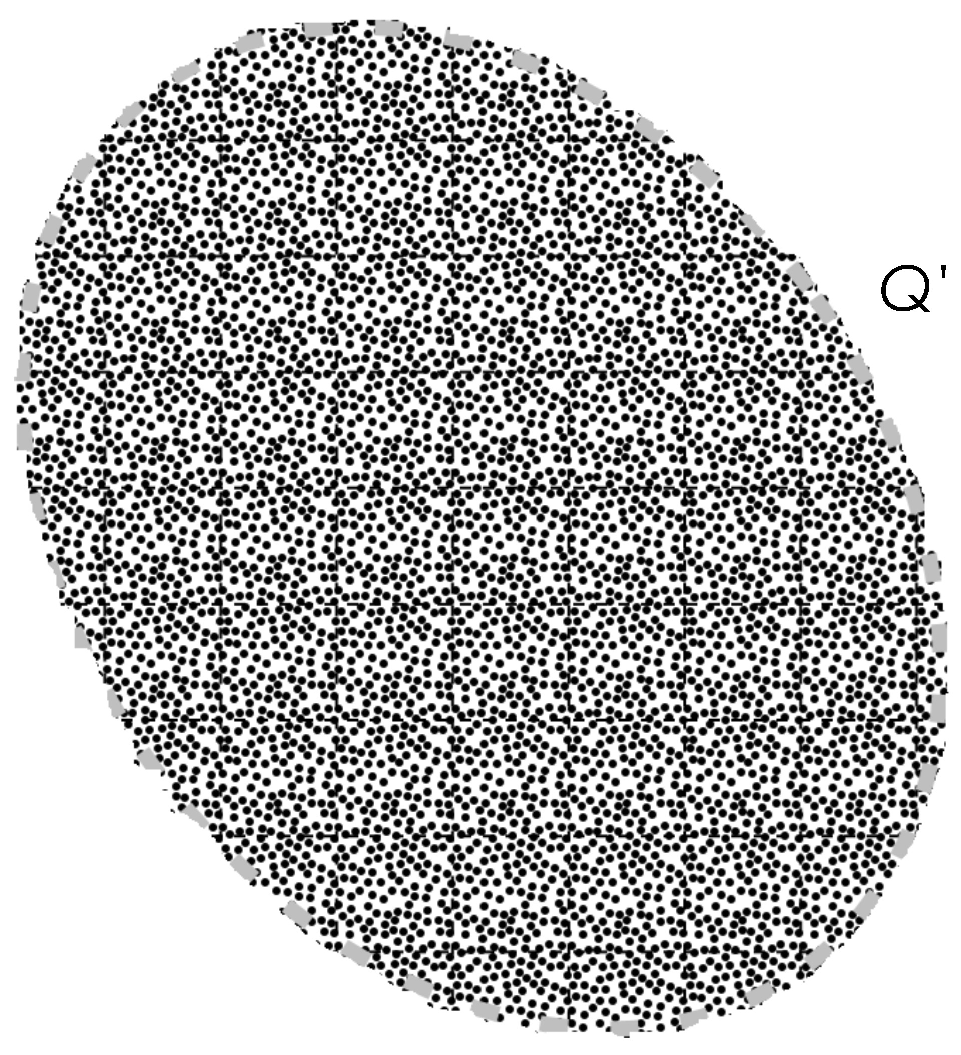
where $m_j$ runs over the integers. A fundamental domain is a subset of the space that contains exactly one point from all its translation images, such as a parallelogram formed by the vectors ${\mathit{\omega }}_{\mathit{j}}$ ($j=1,2$). The concept of homogenization for periodic composite materials is illustrated in Figure 1 for periodic, where the fundamental domain (small cell) Q is periodically continued up to the large sample $Q^{\prime }$. The same conception of the fundamental domain Q holds in ${\mathbb{R}}^3$.

The local conductivity $\mathit{\lambda }\left(\mathbf{x}\right)$ satisfies the following condition:

$$\mathit{\lambda }(\mathbf{x}+{\mathit{\omega }}_j)=\lambda \left(\mathbf{x}\right)(j=1,2).$$

(2)

Substitution of the Equation (1) into the divergence-free condition $\nabla ·\mathbf{q}=0$ yields the second-order elliptic partial differential equation

$$\nabla ·(\mathit{\lambda }\left(\mathbf{x}\right)\nabla T)=0,\mathbf{x}\in Q^{\prime }.$$

(3)

The principles of homogenization are deduced from the multiple-scale analysis. It requires introducing the so-called slow and fast, independent spatial variables. A homogeneous medium with effective properties at the macroscale level gives the same response to a “slow” perturbations of the original heterogeneous medium. The “fast” variable determines the effective properties through a periodic boundary value problem. At the same time, the typical size of a “slow” variable is much larger than the size of periodically repeated cells, described by the “fast” variable. The “slow” variable corresponds to the homogenized composite.

The following mathematical visualization represented in Figure 1 can precisely describe this approach. The sample $Q^{\prime }$ is considered on the macroscale. Let this sample be periodic on a microscale. The fast variable $\mathbf{y}={\epsilon }^{-1}\mathbf{x}$ is introduced, where $\epsilon$ denotes a small positive parameter. The variables $\mathbf{x}$ and $\mathbf{y}$ are assumed to be independent. Introduce the square periodicity cell on the microscale:

$$Q=\{\mathbf{x}=(x_1,x_2)\in Q^{\prime }:-{\displaystyle \frac{\epsilon }{2}}<x_j<{\displaystyle \frac{\epsilon }{2}}(j=1,2)\}.$$

(4)

The cell Q is defined by two fundamental vectors. The two vectors are denoted as ${\mathit{\omega }}_1^{\prime }=\epsilon {\mathit{\omega }}_1$ and ${\mathit{\omega }}_2^{\prime }=\epsilon {\mathit{\omega }}_2$, where ${\mathit{\omega }}_1=(1,0)$ and ${\mathit{\omega }}_2=(0,1)$.

Let us decompose the temperature distribution onto slow and highly oscillated parts:

$$T\left(\mathbf{x}\right)=u_0\left(\mathbf{x}\right)+\epsilon u(\mathbf{x},\mathbf{y}).$$

(5)

Then, the differential operator becomes

$${\displaystyle \frac{d}{d{x}_i}}={\displaystyle \frac{\partial }{\partial x_i}}+{\epsilon }^{-1}{\displaystyle \frac{\partial }{\partial y_i}},$$

(6)

and the operator

$$A_{\epsilon }\equiv {\nabla }_{\mathbf{x}}·\left(\mathit{\lambda }\left({\epsilon }^{-1}\mathbf{x}\right){\nabla }_{\mathbf{x}}\right)={\epsilon }^{-2}{A}_1+{\epsilon }^{-1}{A}_2+A_3,$$

(7)

where the main term

$$A_1={\nabla }_{\mathbf{y}}·\left(\mathit{\lambda }\left(\mathbf{y}\right){\nabla }_{\mathbf{y}}\right).$$

(8)

The main task of homogenization theory is to study the limit boundary value problem for $Q^{\prime }$ when $\epsilon \to 0$. The solution of the boundary value problem (3) converges to a solution to the averaged boundary value problem. The results of convergence, corresponding to $T\left(\mathbf{x}\right)$ in a Sobolev space and to the flux (1) in the Lebesgue space $L^2\left(Q^{\prime }\right)$, reflect the clear physical fact that the macroscopic behavior of the sample $Q^{\prime }$ is described by the effective constant tensor ${\mathit{\lambda }}_e$. Homogenization theory deals with the limit case $\epsilon \to 0$. The effect of the finite small parameter $\epsilon$ is discussed in [39].

It is convenient to present the results of homogenization theory by rescaling the sample size $Q^{\prime }$ and the small periodicity cell Q. Instead of the limit $\epsilon \to 0$, we will consider the equivalent limit when the area of Q is fixed and normalized to unity, and the sample boundary $\partial Q^{\prime }$ tends to infinity. Therefore, the boundary $\partial Q^{\prime }\to \infty$ is considered.

The next result of homogenization theory asserts that the tensor ${\mathit{\lambda }}_e$ can be found from the problem for a doubly periodic composite represented by the small cell Q:

$$\nabla ·\left(\mathit{\lambda }\left(\mathbf{x}\right)\nabla u\left(\mathbf{x}\right)\right)=0,\mathbf{x}\in Q,$$

(9)

with the jump conditions per cell:

$$u(\mathbf{x}+{\mathit{\omega }}_j)-u\left(\mathbf{x}\right)={\xi }_j(j=1,2),$$

(10)

where ${\xi }_j$ are given constants. Sometimes, the constants ${\xi }_j$ are introduced into the differential equation Equation (9) by the substitution $u_j\left(\mathbf{x}\right)=u\left(\mathbf{x}\right)+{\xi }_j{x}_j$ ($j=1,2$). Here, $\mathbf{x}=(x_1,x_2)$. The problems (9) and (10) become

$$\nabla ·\left[\mathit{\lambda }\left(\mathbf{x}\right)(\nabla u_j\left(\mathbf{x}\right)+{\xi }_j)\right]=0,\mathbf{x}\in Q,$$

(11)

$$u_j(\mathbf{x}+{\mathit{\omega }}_j)-u_j\left(\mathbf{x}\right)=0(j=1,2).$$

(12)

A dispersed composite can be described by the cell $Q=D\cup D^{+}\cup \partial D^{+}$, where $D^{+}={\cup }_{k=1}^N{D}_k$ denotes the union of inclusions, $\partial D^{+}$ the union of their boundaries, and D the host domain. The parameter f denotes the concentration of inclusions. It is introduced as the ratio of areas (volumes) $f={\displaystyle \frac{|D^{+}|}{\left|Q\right|}}$. A piece-wise constant scalar function

$$\lambda \left(\mathbf{x}\right)=\left\{\begin{array}{cc}{\lambda }_k\hfill & \mathbf{x}\in D_k(k=1,2,\dots ,N)\hfill \\ \lambda =1\hfill & \mathbf{x}\in D\hfill \end{array}\right.$$

(13)

describes a dispersed composite, where the conductivity of D is normalized to unity and the conductivity of $D_k$ is ${\lambda }_k$. The number of inclusions per periodicity cell Q is always equal to N.

Let us introduce the dimensionless contrast parameters:

$${\varrho }_k={\displaystyle \frac{{\lambda }_k-1}{{\lambda }_k+1}}.$$

(14)

The parameter ${\lambda }_k\ge 0$ represents the steady heat conduction and may be complex when referring to the dielectric permittivity. The designation $\varrho$ is used for two-phase composites when ${\lambda }_k={\lambda }_1$ for all k.

For a successful homogenization, one should respect the following homogenization principles:

• In the framework of homogenization theory of composites [7,8,9], Q must be a fundamental domain. In particular, a parallelepiped in ${\mathbb{R}}^3$ is the most suitable to represent the fundamental domain. It is a parallelogram in ${\mathbb{R}}^2$ for the fibrous composite and an interval in $\mathbb{R}$ for the layered composite.
• Periodicity conditions corresponding to the applied external field must be posed on the opposite sides of Q.
• The effective conductivity tensor is determined by averaging the local fields over Q; see, for instance, Formula (20) below.

The local fields in a composite material can be found by solving a boundary value problem considered in the local statement, i.e., for a fragment of the composite with a finite number of inclusions with the corresponding boundary conditions. At the same time, the effective constants of the composite are found by a periodic boundary value problem. In the framework of the periodic problem, one has to consider the composite extended to occupy the whole space. Some empirical methods discussed in Section 1.1 do not satisfy this requirement and lead to misleading results for the effective constants.

3. Concept of Investigations

The preliminary step involves the so-called digital material representation. The latter is based on Image Analysis, not to be discussed in the current paper. We refer the reader to the papers [37,40], involving Image Analysis, and the references therein.

The initial step in the investigation of composites is the consideration of the rigorous Hashin–Shtrikman bounds or other similar bounds of higher order devised for random composites [14,15]. If the bounds are sufficiently tight, one may stop and take the bounds as an ultimate result. In the opposite case, a constructive homogenization might be considered. We outline here the main steps of constructive homogenization in application to dispersed random composites:

• Computation of structural sums.
• Computation of effective conductivity through structural sums.
• Application of Padé approximation to resummation of truncated power series.

The purposes of the above steps are described in the present section. Their implementation will be detailed in the next sections. The structural sums $e_{m_1,m_2,\dots ,m_q}$ ($m_1,m_2,\dots ,m_q=2,3,4,\dots$) arise in the application of the generalized alternating method of Schwarz [21] to a boundary value problem with the further averaging of local fields. A structural sum of order q is written in explicit form as a discrete q-point convolution of Eisenstein functions; see Appendix A. The structural sums for the 2D conductivity of circular disks are explicitly written in Section 5. An algorithm for the fast computation of higher-order structural sums is described in Chapter 2 of the book [35]. The sums $e_{m_1,m_2,\dots ,m_q}$ depend on the gravity centers of the inclusions. If these centers are random, statistical processing must be performed to determine the expected values of $e_{m_1,m_2,\dots ,m_q}$. The same formulas can be applied to the structural sums for other shapes [21].

When we are interested only in classifying all possible structures, the second step may be omitted. It is sufficient to construct finite subsets of the structural sums $\mathcal{E}=\{e_2,e_{22},e_{33},e_{222},\dots \}$ and ${\mathcal{E}}^{\prime }=\{e_2^{\prime },e_{22}^{\prime },e_{33}^{\prime },e_{222}^{\prime },\dots \}$ corresponding to two different structures. In such a manner, one can compare their anisotropy and regularity. Clusters of inclusions can be analyzed as well. Generally speaking, one can employ the sums to classify the structures [35,36]. The formulas for 3D structural sums can be found in [35]. The structural sums for elastic media can be found in [35] and will be discussed in a separate paper (Part II).

After the computation of structural sums, their mean values will be substituted in the series (33) written in Section 5. As a result of cutting, we arrive at an analytical formula for the effective conductivity tensor in a polynomial in f. One can even read in some papers that such a polynomial is an “exact” solution to the problem under consideration. Of course, that is not the correct assertion.

The final step is the resummation of the truncated series [34,35]. Here, we compute critical indices and amplitudes, as well as derive closed-form expressions for effective quantities designed to be applicable for all f.

Remark 1. 

There are special structures for which exact and approximate formulas could be derived by applying special methods. Three approaches, developed by Keller, Dykhne–Keller–Mathéron, and by Hashin–Shtrikman, can be mentioned in this regard. The asymptotically small gap formula derived by Keller led to the theory of structural approximations for densely packed composites [41,42]. The Hashin–Shtrikman assemblages of coated inclusions yielded a series of new complicated composite constructions [43,44]. The Dykhne–Keller–Mathéron approach was extended to multiphase checkerboard structures [45,46].

4. Deterministic Composite

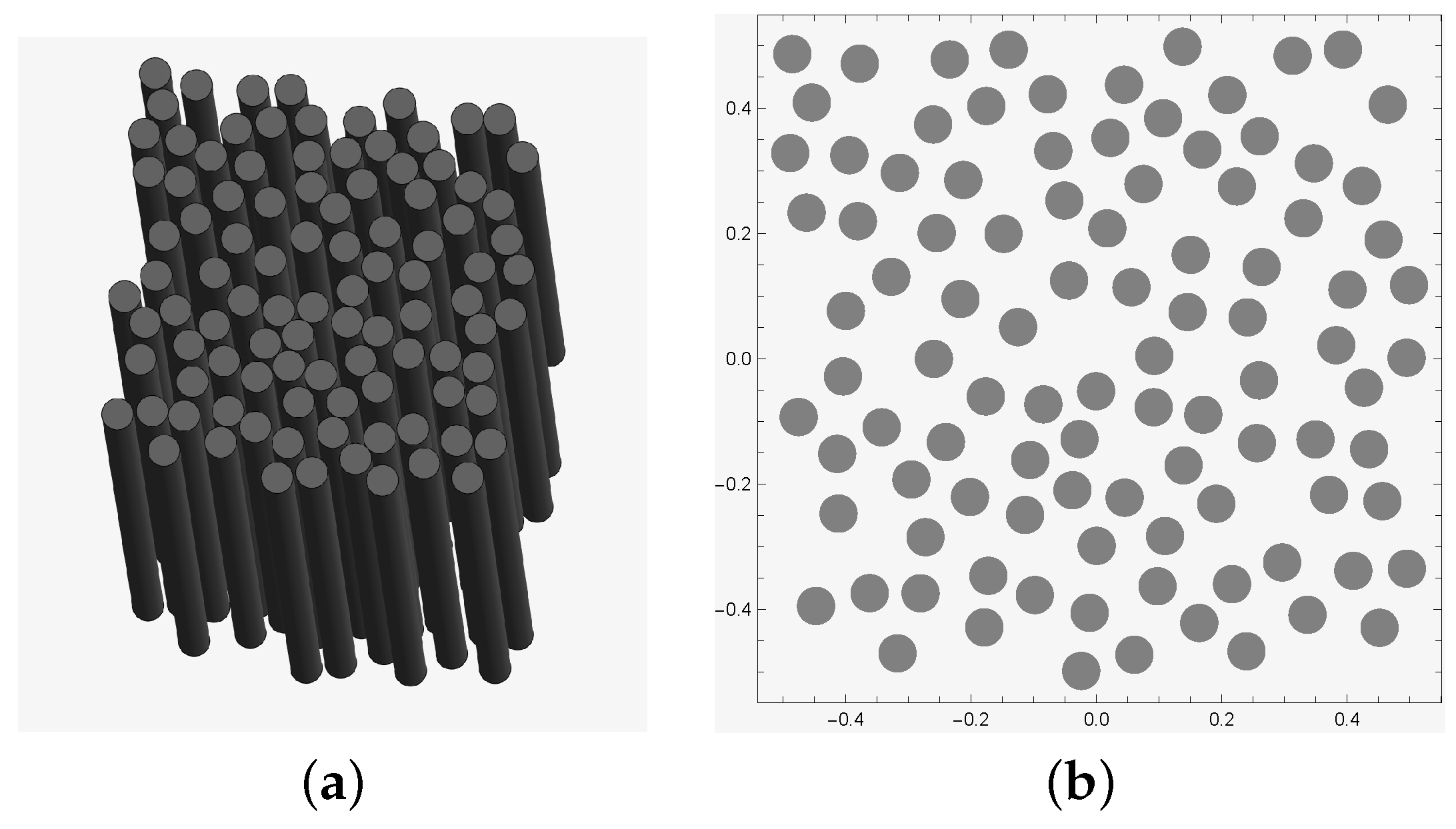
Consider the infinite double periodic unidirectional array of cylinder fibers depicted in Figure 2, represented by the square $Q=\{(x_1,x_2)\in {\mathbb{R}}^2:-{\displaystyle \frac{1}{2}}<x_j<{\displaystyle \frac{1}{2}}\}$. The square contains N equal circular inclusions of radius r distributed without overlap. Let the coordinates of circular inclusions and their radius r be known and fixed. This is an example of a deterministic composite material since its geometry is fixed and precisely defined. Let the square cell Q periodically extend to the plane ${\mathbb{R}}^2$. Therefore, the homogenization principles are satisfied, and one can state the proper periodicity problem to determine the effective constants.

The following conditions on the potential $u(x_1,x_2)$ in the host can be considered:

$$u(x_1+1,x_2)-u(x_1,x_2)=1,u(x_1,x_2+1)-u(x_1,x_2)=0.$$

(15)

The condition (15) means that the external flux parallel to the axis $x_1$ is applied to the square array:

$${\mathbf{q}}_{ext}=-(1,0).$$

(16)

The temperature jump equals 1 along the axis $x_1$ and 0 along the axis $x_2$. The conditions of the perfect contact have the form

$$u\left(\mathbf{x}\right)=u_1\left(\mathbf{x}\right),{\displaystyle \frac{\partial u}{\partial \mathbf{n}}}\left(\mathbf{x}\right)={\lambda }_1{\displaystyle \frac{\partial u_1}{\partial \mathbf{n}}}\left(\mathbf{x}\right)\mathrm{on}\partial D^{+}.$$

(17)

In the considered case, the quasi-periodicity conditions (15) can be replaced with the boundary conditions for the domain Q:

$$u\left(\pm {\displaystyle \frac{1}{2}},x_2\right)=\pm {\displaystyle \frac{1}{2}},{\displaystyle \frac{\partial u}{\partial x_2}}\left(x_1,\pm {\displaystyle \frac{1}{2}}\right)=0.$$

(18)

The effective conductivity tensor ${\mathit{\lambda }}_e$ can be determined by the averaged value over Q:

$$\langle f\left(\mathbf{x}\right)\rangle ={\displaystyle \frac{1}{\left|Q\right|}}{\int }_{Q}f\left(\mathbf{x}\right)d\mathbf{x}.$$

(19)

The value $\langle \mathbf{q}\rangle$ stands for the averaged flux and $\widehat{\nabla u}$ is the macroscopic temperature gradient over the considered sample. In the case of Equation (16), $\widehat{\nabla u}=(1,0)$ and $\langle \mathbf{q}\rangle ={\mathbf{q}}_{ext}$. The effective conductivity tensor ${\mathit{\lambda }}_e$ in the case of the perfect contact between inclusions and host is defined as the proportionality coefficient in equation [34]:

$$\langle \mathbf{q}\rangle =-{\mathit{\lambda }}_e\widehat{\nabla u}.$$

(20)

This approach is similar to the black box operator discussed in [23], meaning that the input is given by $\widehat{\nabla u}$, and the output $\langle \mathbf{q}\rangle$ ought to be measured or calculated. The tensor ${\mathit{\lambda }}_e$ determines the conductive properties of the sample Q.

Equation (20) is linear. It relates two constant vectors $\langle \mathbf{q}\rangle$ and $\widehat{\nabla u}$ in ${\mathbb{R}}^3$. It follows from linear algebra that a general linear relation between two vectors is determined by a matrix called the effective conductivity tensor:

$${\mathit{\lambda }}_e=\left(\begin{array}{c}{\lambda }_{11}{\lambda }_{12}{\lambda }_{13}\hfill \\ {\lambda }_{21}{\lambda }_{22}{\lambda }_{23}\hfill \\ {\lambda }_{31}{\lambda }_{32}{\lambda }_{33}\hfill \end{array}\right).$$

(21)

The tensor (21) is symmetric, ${\lambda }_{ij}={\lambda }_{ji}$. Hence, it can be reduced to the diagonal form. The tensor ${\mathit{\lambda }}_e$ expresses the anisotropic effective properties of the homogenized material, i.e., different conductivity in different directions.

Let the matrix Equation (21) be represented in the form ${\mathit{\lambda }}_e={\lambda }_e\mathbf{I}$, where $\mathbf{I}$ denotes the unit matrix. In this case, the material is isotropic macroscopically, and the scalar ${\lambda }_e$ is called the effective conductivity of the composite material. The same statements hold in the case of heat conduction perpendicular to the unidirectional fibrous materials, depicted in Figure 2 and Figure 3. Then, the above equations are decomposed into 1D and 2D problems, and the tensor (21) becomes

$${\mathit{\lambda }}_e=\left(\begin{array}{c}{\lambda }_{11}{\lambda }_{12}0\hfill \\ {\lambda }_{21}{\lambda }_{22}0\hfill \\ 00{\lambda }_{33}\hfill \end{array}\right),$$

(22)

where ${\lambda }_{33}={\lambda }_{1}f+(1-f)$. The 2D effective conductivity tensor is introduced in this case:

$${\mathit{\lambda }}_e^{2D}=\left(\begin{array}{c}{\lambda }_{11}{\lambda }_{12}\hfill \\ {\lambda }_{21}{\lambda }_{22}\hfill \end{array}\right)$$

(23)

denoted for shortness by ${\mathit{\lambda }}_e$.

5. Step 1: Computation of Structural Sums

The dependence of effective constants on shapes and locations was established in [21]. So, we are able to write an approximate analytical formula for the effective conductivity tensor (23) for 2D two-phase composites with circular inclusions.

Let a composite be represented by a periodicity cell Q formed by the two fundamental translations defined by the vectors denoted as ${\omega }_1$ and ${\omega }_2$ defined on the complex plane $\mathbb{C}$:

$$Q=\left\{z=t_1{\omega }_1+t_2{\omega }_2\in \mathbb{C}:-{\displaystyle \frac{1}{2}}<t_1,t_2<{\displaystyle \frac{1}{2}}\right\}.$$

(24)

Without loss of generality, the periods ${\omega }_1$ and ${\omega }_2$ satisfy the conditions ${\omega }_1>0$ and $\mathrm{Im}{\omega }_2>0$. Let us normalize the area of Q to unity, so that ${\omega }_1\mathrm{Im}{\omega }_2=1.$ Let $\mathrm{i}=\sqrt{-1}$ be the imaginary unit. We will consider below the particular cases of lattices, such as the hexagonal lattice with

$${\omega }_1={\displaystyle \frac{\sqrt{2}}{\sqrt[4]{3}}},{\omega }_2={\displaystyle \frac{\sqrt{2}}{\sqrt[4]{3}}}{\displaystyle \frac{1+\mathrm{i}\sqrt{3}}{2}},$$

(25)

and the square lattice with

$${\omega }_1=1,{\omega }_2=\mathrm{i}.$$

(26)

The considered doubly periodic structure can be represented by a plane torus denoted by $\mathcal{Q}=\left\{Q+m_1{\omega }_1+m_2{\omega }_2:m_1,m_2\in \mathbb{Z}\right\}$, where $\mathbb{Z}$ denotes the set of integers. Introduce the lattice sums [47]:

$$S_p=\sum _{(m_1,m_2)\in {\mathbb{Z}}^2\setminus (m_1,m_2)\ne (0,0)}{\displaystyle \frac{1}{{(m_1{\omega }_1+m_2{\omega }_2)}^p}},p=2,3,\dots .$$

(27)

The conditionally convergent sum $S_2$ is defined by the Eisenstein summation method [47], and $S_2=\pi$ for the square and hexagonal arrays. The exact and recurrence formulas for the lattice sums can be found both in Appendix A.

Consider N mutually disjoint disks $D_k=\{z\in \mathbb{C}:|z-a_k|<r\}$, where $a_k$ denotes the center of $D_k$ in Q and $r_k$ its radius. Let $D=Q\setminus {\cup }_{k=1}^N(D_k\cup L_k)$ denote the complement of all the closures of $D_k$ to Q. An example of disks $D_k$ is shown in Figure 2b.

We will use below the Eisenstein functions $E_p\left(z\right)$ ($p=2,3,\dots$) related to the elliptic Weierstrass functions in the following way [34]:

$$E_2\left(z\right)=\wp \left(z\right)+S_2,E_p\left(z\right)=-{\displaystyle \frac{{(-1)}^p}{(p-1)!}}{\displaystyle \frac{{\mathrm{d}}^{p-2}\wp \left(z\right)}{\mathrm{d}{z}^{p-2}}},p=3,4,\dots$$

(28)

Following [34] (Chapter 4), let us introduce the structural sums

$$\begin{array}{c}{e}_{m_1,\dots ,m_q}={\displaystyle \frac{1}{N^{\frac{\alpha }{2}+1}}}\sum _{k_0,k_1,\dots ,k_n}{E}_{m_1}(a_{k_0}-a_{k_1})\mathbf{C}{E}_{m_2}(a_{k_1}-a_{k_2})\dots {\mathbf{C}}^{q+1}{E}_{m_q}(a_{k_{q-1}}-a_{k_q}),\hfill \end{array}$$

(29)

where $\alpha =m_1+\cdots +m_q$. It is assumed for shortness that

$$E_p(a_k-a_m)=:S_p\mathrm{and}\wp (a_k-a_m):=0,\mathrm{for}{a}_m=a_k(m,k=1,2,\dots ,N).$$

(30)

For instance, $e_2$ takes the following form:

$$e_2={\displaystyle \frac{1}{N^2}}\sum _{k,m=1}^N{E}_2(a_k-a_m)\equiv \pi +{\displaystyle \frac{1}{N^2}}\sum _{k,m=1}^N\wp (a_k-a_m).$$

(31)

The structural sums, including $e_2$ and their relations to macroscopic anisotropy, were discussed in [37]. A set of relations among the structural sums for macroscopically isotropic composites was established. In particular, the isotropy is maintained up to $O\left(f^3\right)$ when $e_2=\pi$.

Using the complex structural sums, we form the matrix structural sums:

$${\mathbf{e}}_{m_1,\dots ,m_q}=\left(\begin{array}{cc}\mathrm{Re}{e}_{m_1,\dots ,m_q}\hfill & -\mathrm{Im}{e}_{m_1,\dots ,m_q}\hfill \\ -\mathrm{Im}{e}_{m_1,\dots ,m_q}\hfill & \mathrm{Re}{e}_{m_1,\dots ,m_q}^{\ast }\hfill \end{array}\right),$$

(32)

where $e_{m_1,\dots ,m_q}^{\ast }$ has the same form except at the terms $E_2(a_k-a_m)$, which have to be replaced by the expressions $2\pi -E_2(a_k-a_m)$.

The effective conductivity tensor has the form [34]:

$${\mathit{\lambda }}_e=(1+2\varrho f)\mathbf{I}+2\varrho f({\mathbf{A}}_{1}f+{\mathbf{A}}_2{f}^2+\cdots ),$$

(33)

where a few first matrices are written below:

$$\begin{array}{ccc}\hfill {\mathbf{A}}_1& =& {\displaystyle \frac{\varrho }{\pi }}{\mathbf{e}}_2,{\mathbf{A}}_2={\displaystyle \frac{{\varrho }^2}{{\pi }^2}}{\mathbf{e}}_{22},{\mathbf{A}}_3={\displaystyle \frac{{\varrho }^2}{{\pi }^3}}\left[-2{\mathbf{e}}_{33}+\varrho {\mathbf{e}}_{222}\right],\hfill \\ \hfill {\mathbf{A}}_4& =& {\displaystyle \frac{{\varrho }^2}{{\pi }^4}}\left[3{\mathbf{e}}_{44}-4\varrho {\mathbf{e}}_{332}+{\varrho }^2{\mathbf{e}}_{2222}\right],\hfill \\ \hfill {\mathbf{A}}_5& =& {\displaystyle \frac{{\varrho }^2}{{\pi }^5}}\left[-4{\mathbf{e}}_{55}+6\varrho ({\mathbf{e}}_{442}+2{\mathbf{e}}_{343})-2{\varrho }^2({\mathbf{e}}_{2332}+2\mathrm{Re}{\mathbf{e}}_{2233})+{\varrho }^3{\mathbf{e}}_{22222}\right],\hfill \\ \hfill {\mathbf{A}}_6& =& {\displaystyle \frac{{\varrho }^2}{{\pi }^6}}\left[5{\mathbf{e}}_{66}-8\varrho ({\mathbf{e}}_{255}+3{\mathbf{e}}_{354})\right.\hfill \\ & & +{\varrho }^2(6\mathrm{Re}{\mathbf{e}}_{2244}+12\mathrm{Re}{\mathbf{e}}_{2343}+4{\mathbf{e}}_{3333}+3{\mathbf{e}}_{2442})-\hfill \\ & & \left.-4{\varrho }^3({\mathbf{e}}_{22233}+{\mathbf{e}}_{22332})+{\varrho }^4{\mathbf{e}}_{222222}\right],\hfill \end{array}$$

(34)

$$\begin{array}{ccc}\hfill {\mathbf{A}}_7& =& {\displaystyle \frac{{\varrho }^2}{{\pi }^7}}[-6{\mathbf{e}}_{77}+10\varrho \left({\mathbf{e}}_{266}+4{\mathbf{e}}_{365}+3{\mathbf{e}}_{464}\right)\hfill \\ & & (-2{\varrho }^{2}2{\mathbf{e}}_{2255}+6{\mathbf{e}}_{2354}+6{\mathbf{e}}_{2453}+2{\mathbf{e}}_{2552}+3{\mathbf{e}}_{3344}+9{\mathbf{e}}_{3443}\hfill \\ \hfill & & \left.+6{\mathbf{e}}_{3542}+3{\mathbf{e}}_{4433}+6{\mathbf{e}}_{4532}+2{\mathbf{e}}_{5522}\right)\hfill \\ \hfill & & +2{\varrho }^3(3\mathrm{Re}{\mathbf{e}}_{22244}+6\mathrm{Re}{\mathbf{e}}_{22343}+3\mathrm{Re}{\mathbf{e}}_{22442}+4\mathrm{Re}{\mathbf{e}}_{23333}\hfill \\ \hfill & & \left.+3{\mathbf{e}}_{23432}+2{\mathbf{e}}_{33233}\right)-2{\varrho }^4\left(2{\mathbf{e}}_{222233}+2{\mathbf{e}}_{222332}+{\mathbf{e}}_{223322}\right)\left.+{\varrho }^5{\mathbf{e}}_{2222222}\right].\hfill \end{array}$$

$$\begin{array}{ccc}\hfill {\mathbf{A}}_8& =& {\displaystyle \frac{{\varrho }^2}{{\pi }^8}}[7{\mathbf{e}}_{88}+{\varrho }^4\mathrm{Re}(6{\mathbf{e}}_{244222}+8{\mathbf{e}}_{333322}+6{\mathbf{e}}_{442222})+16{\varrho }^2\mathrm{Re}{\mathbf{e}}_{5533}\hfill \\ \hfill & & -2{\varrho }^5({\mathbf{e}}_{2223322}+2{\mathbf{e}}_{2233222}+4{\mathbf{e}}_{2332222}+4{\mathbf{e}}_{3322222})+{\varrho }^4(6{\mathbf{e}}_{222343}\hfill \\ \hfill & & +6{\mathbf{e}}_{223432}+3{\mathbf{e}}_{224422}+4{\mathbf{e}}_{233233}+4{\mathbf{e}}_{233332}+6{\mathbf{e}}_{234322}+4{\mathbf{e}}_{332233}\hfill \\ \hfill & & +4{\mathbf{e}}_{332332}+6{\mathbf{e}}_{343222})-{\varrho }^3(12{\mathbf{e}}_{22354}+12{\mathbf{e}}_{22453}+6{\varrho }^3{\mathbf{e}}_{23344}+18{\mathbf{e}}_{23443}\hfill \\ \hfill & & +12{\mathbf{e}}_{23542}+6{\mathbf{e}}_{24433}+12{\mathbf{e}}_{24532}+8{\mathbf{e}}_{25522}+12{\mathbf{e}}_{33343}+6{\mathbf{e}}_{33442}+12{\mathbf{e}}_{34333}\hfill \\ \hfill & & +18{\mathbf{e}}_{34432}+12{\mathbf{e}}_{35422}+12{\mathbf{e}}_{44233}+6{\mathbf{e}}_{44332}+12{\mathbf{e}}_{45322}+8{\mathbf{e}}_{55222})\hfill \\ \hfill & & +{\varrho }^2(20{\mathbf{e}}_{2365}+30{\mathbf{e}}_{2464}+20{\mathbf{e}}_{2563}+5{\mathbf{e}}_{2662}+36{\mathbf{e}}_{3454}+48{\mathbf{e}}_{3553}+20{\mathbf{e}}_{3652}\hfill \\ \hfill & & +9{\mathbf{e}}_{4444}+36{\mathbf{e}}_{4543}+30{\mathbf{e}}_{4642}+20{\mathbf{e}}_{5632}+10{\mathbf{e}}_{6622})\hfill \\ \hfill & & -\varrho (30{\mathbf{e}}_{376}+60\varrho {\mathbf{e}}_{475}+60\varrho {\mathbf{e}}_{574}+30\varrho {\mathbf{e}}_{673}+12\varrho {\mathbf{e}}_{772})+{\varrho }^6{\mathbf{e}}_{22222222}].\hfill \end{array}$$

Here, the numbers in the subscripts are not divided by commas for shortness. The first-order term in Equation (33) corresponds to the famous Clausius–Mossotti approximation.

It was established in [34] that for macroscopically isotropic composites,

$$e_2=\pi ,e_{222}=2\pi e_{22}-{\pi }^3,e_{332}=\pi e_{33}.$$

(35)

Moreover, the following useful formulas were derived in [34]:

$$e_{pp}={\displaystyle \frac{{(-1)}^p}{N^{p+1}}}\sum _{k=1}^N{\left|\sum _{m=1}^N{E}_p(a_k-a_m)\right|}^2(p=2,3,\dots ),$$

(36)

$$e_{2222}={\displaystyle \frac{1}{N^5}}\sum _{k_0=1}^N{\left|\sum _{k_1,k_2=1}^N{E}_2(a_{k_0}-a_{k_1})\overline{E_2(a_{k_1}-a_{k_2})}\right|}^2.$$

(37)

The Formulas (33) and (34) represent the decomposition of the tensor ${\mathit{\lambda }}_e$. The latter tensor is separated into two terms, arising from purely physical and geometrical considerations, respectively. The series (33) is an expansion in terms of concentration f. The coefficients of this expansion $2\varrho {\mathbf{A}}_j$ are linear combinations of structural sums $e_{m_1,\dots ,m_q}$. The coefficients involved in the sums (34) are polynomials in the contrast parameter $\varrho$.

6. Step 2: Computation of Effective Conductivity Through the Structural Sums

The notion of randomness in application to composites means that the tensor, or matrix function, $\mathit{\lambda }\left(\mathbf{x}\right)$ is a random function dependent on the spatial variable $\mathbf{x}$ in the plane ${\mathbb{R}}^2$ (space ${\mathbb{R}}^3$). The matrix function $\mathit{\lambda }\left(\mathbf{x}\right)$ must be statistically homogeneous in the plane ${\mathbb{R}}^2$ [9,28,48,49]. This is the necessary and sufficient condition for converging the local fields governed by Equation (9) as $\partial Q^{\prime }$ tends to an infinite point. This convergence yields the existence of effective constants of the statistically homogeneous tensor $\mathit{\lambda }\left(\mathbf{x}\right)$ defined in the plane ${\mathbb{R}}^2$.

A random composite is not necessarily doubly periodical, but it is stochastically periodic. The latter means that the matrix function $\mathit{\lambda }\left(\mathbf{x}\right)$ is statistically homogeneous by definition if it has the same probabilistic distribution under translation $z\mapsto z+\mathit{\omega }$ for any $\mathit{\omega }$.

A dispersed random composite is formed when an infinite collection of inclusions ${\mathbf{D}}_k$ with the prescribed conductivity ${\lambda }_k$ ($k=1,2,\dots$) is given, but their locations and areas are random. Namely, their gravitational centers

$$\mathcal{A}=\{{\mathbf{a}}_1,{\mathbf{a}}_2,\dots \}$$

(38)

and their areas $\left\{\right|{\mathbf{D}}_1|,|{\mathbf{D}}_2|,\dots \}$ are chosen at random. In the case of identical circular inclusions, their radius r, the contrast parameter $\varrho$, and the concentration f can acquire deterministic or random values.

Consider disks of equal size distributed without overlaps in the plane ${\mathbb{R}}^2$. Let f, $\varrho$, and r be fixed. Let the geometric distribution of the centers (38) form a statistically homogeneous field. In particular, the centers $\mathcal{A}$ can form a doubly periodic set $\mathcal{A}=\{{\mathbf{a}}_1,{\mathbf{a}}_2,\dots ,{\mathbf{a}}_N\}$ with a fixed number of inclusions N per cell Q. In this case, we consider the random set of N circular inclusions distributed without overlaps in the torus topology. Any distribution of N disks is a statistically homogeneous field in Q, assuming its periodic extension to the whole plane. Random composites do not necessarily have to be strictly periodic. However, the periodicity must be stochastic, meaning that the geometric (probabilistic) distribution of inclusions is the same under parallel translations.

The case of a cell of unknown periodicity, including the unknown number of inclusions per cell N, was investigated in [34]. In the book [34] and the works cited therein, an analytical theory of the representative volume cell (aRVE) was suggested. The analytical theory demonstrates the variety of dispersed composites with circular (spherical) inclusions. It extends the naive theory of RVE, by concentrating on the unique minimal number N per RVE cell and hence on the unique formula for the dispersed random composite materials.

In addition, the general constructive method [34] was suggested in such a way that even the same statistical generation of inclusions may lead to different results for effective constants. We summarize the simulations of random composite arrays using some protocols [34,35] corresponding to uniform disks positioned on the plane without overlaps.

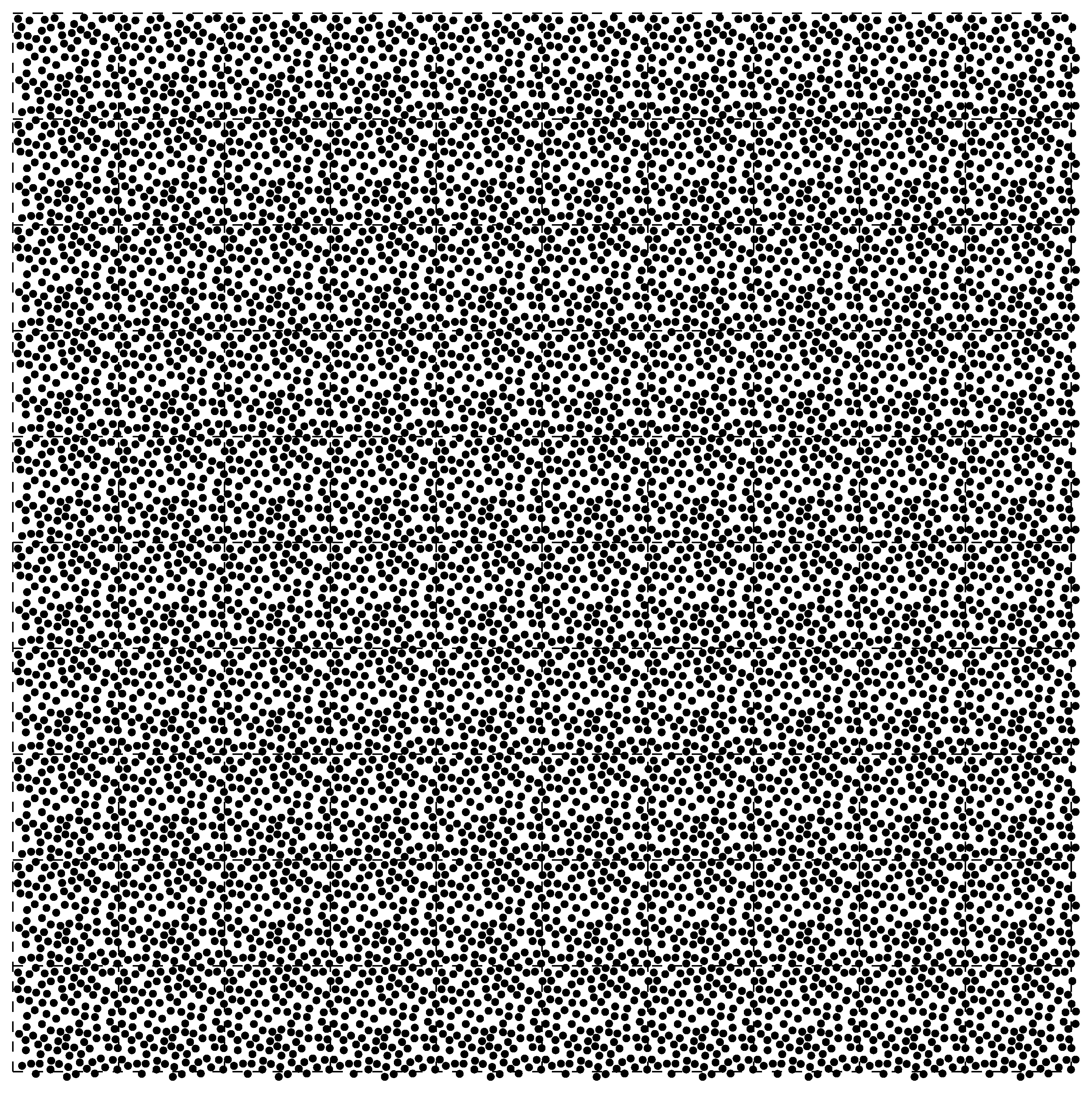
The RW protocols use Monte Carlo simulations to generate a statistical configuration. Initially, inclusion centers are placed at regular lattice nodes within the unit periodicity cell Q and subjected to random motion to prevent overlap. The system evolves until it reaches a statistically steady state, forming a doubly periodic set of discs distributed uniformly without overlaps. This configuration is used to compute the effective coefficients, providing a robust numerical characterization of the material. The RWs method is particularly effective for modeling systems with high concentrations of inclusions, ensuring uniformity and stability over extended domains.

The RSA protocol is a sequential process that could be applied at moderately high concentrations up to $f=0.5773$ in two-dimensional composites. In this approach, inclusions are placed incrementally. A random point within Q is selected as the center of the initial inclusion. Each subsequent center is chosen statistically uniformly, excluding regions occupied by previous inclusions to prevent overlap. The probability distribution for each new center depends on the positions of earlier inclusions. This process continues until the desired number of inclusions is placed.

There is also a special case where the inclusion conductivity is much higher than the conductivity ($\varrho =1$) of the host [20]. Below, the expansion for such high-contrast materials is presented in the truncated numerical form by use of the RSA protocol, see Formula (9.1.2) from [20,34]:

$${\lambda }_e^{RSA}=1+2f+2f^2+5.13057f^3+5.9969f^4+{\Delta }_{RSA}\left(f\right)$$

(39)

and by random walk, see Formula (9.2.37) from [20,34]:

$${\lambda }_e^{RW}=1+2f+2f^2+5.00392f^3+6.3495f^4+{\Delta }_{RW}\left(f\right).$$

(40)

The remainders ${\Delta }_{RSA}\left(f\right)$ and ${\Delta }_{RW}\left(f\right)$ have highly irregular forms and do not contribute to the critical properties. For instance, the coefficients on $f^k$ ($k=5,6,7,8$) in the term ${\Delta }_{RSA}\left(f\right)$ are of order ${10}^{-10}$, see the estimation [34] (Formula (9.1.3)) of other terms. The mean values of the above coefficients do vanish, but their moduli are greater than two.

Random walks in the RW protocol start with the perfect hexagonal arrangement that has the maximum packing array with concentration $f_c={\displaystyle \frac{\pi }{\sqrt{12}}}\approx 0.9069$. Therefore, this protocol admits the percolation regime of touching disks and [34]:

$${\lambda }_e\simeq B{(f_c-f)}^{-s},\mathrm{as}f\to f_c.$$

(41)

The critical index $s\approx 1.3$, while the critical amplitude B was estimated as $B\approx 1.71$ [34].

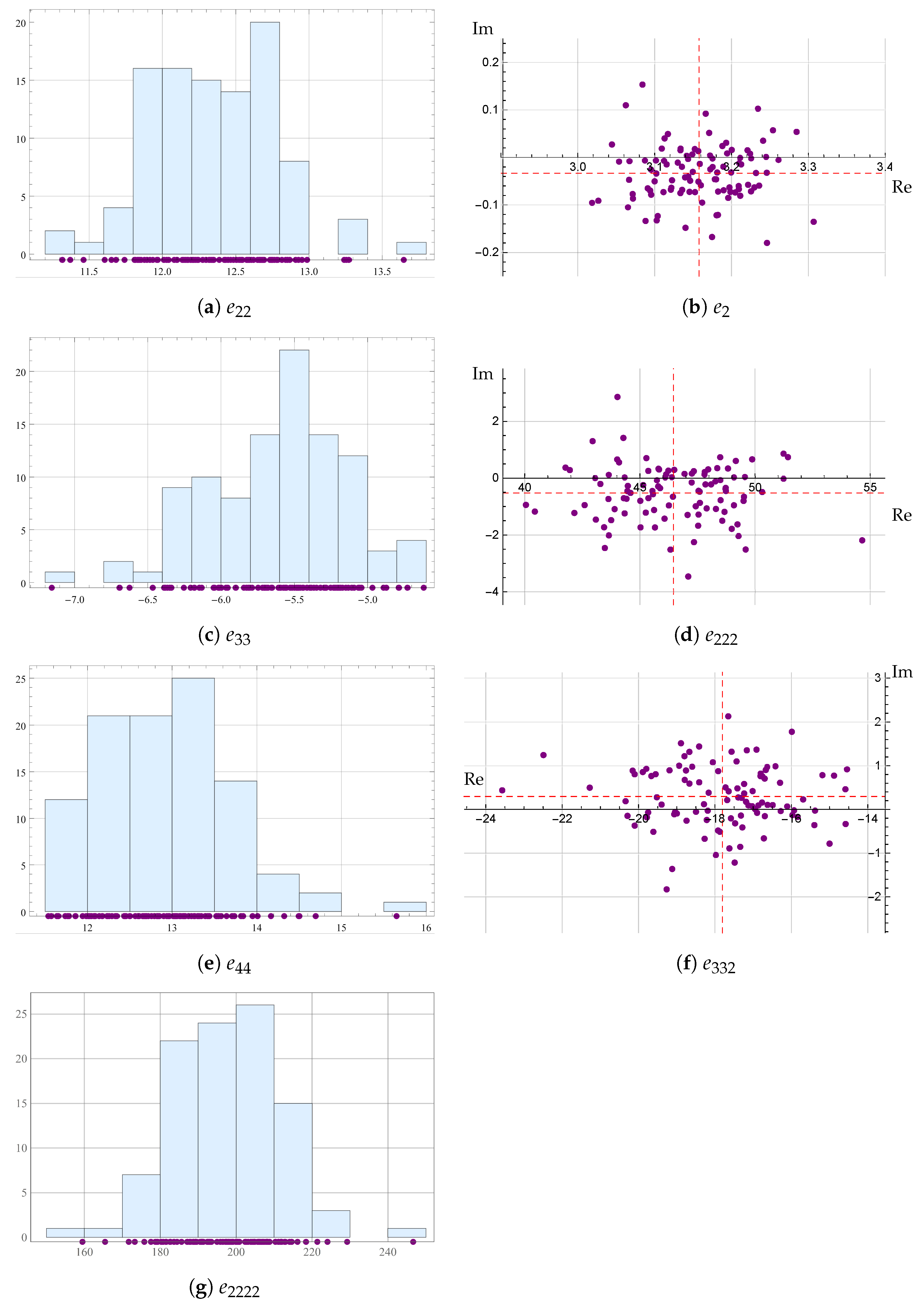
We now consider another, the so-called RSA protocol near the concentration $f=0.126$. More precisely, we generate 100 disks of radius $r=0.02$ distributed without overlaps in the unit square Q using the RSA method and calculate the effective conductivity by Equations (33) and (34). This computational experiment is repeated 50 times. The averaged result of computations has the form

$${\lambda }_{sq}^{RSA}\left(0.126\right)=1+2f+2f^2+5.21269f^3+16.1938f^4+62.5597f^5+O\left(f^6\right).$$

(42)

It should be noted that the coefficients of ${\lambda }_e^{RSA}\left(0.126\right)$ and ${\lambda }_e^{RSA}$ in $f^3$ differ, and the coefficients in $f^4$ differ significantly. Moreover, the term of the order of $f^5$ is highly irregular in ${\lambda }_e^{RSA}$. At the same time, this term in ${\lambda }_e^{RSA}\left(0.126\right)$ is more stable.

After performing 50 independent simulations with 300 disks by RSA for the square and hexagonal arrays, the mean polynomials for the effective conductivity are obtained. In particular,

$$\begin{array}{c}{\lambda }_{sq}^{RSA}(\varrho ,0.377)=1+2f\varrho +2f^2{\varrho }^2+2.48277f^3{\varrho }^3+0.720739f^4{\varrho }^3+0.813692f^5{\varrho }^3\hfill \\ \\ +2.96542f^4{\varrho }^4+1.44148f^5{\varrho }^4+4.01997f^5{\varrho }^5+O\left(f^6\right).\hfill \end{array}$$

(43)

Substituting $\varrho =1$ into Equation (43) yields

$${\lambda }_{sq}^{RSA}\left(0.377\right)=1+2f+2f^2+2.48277f^3+3.68616f^4+6.27514f^5+O\left(f^6\right).$$

(44)

Almost the same results hold for the hexagonal array:

$$\begin{array}{c}{\lambda }_{hex}^{RSA}(\varrho ,0.377)=1+2f\varrho +2f^2{\varrho }^2+2.48155f^3{\varrho }^3+0.725247f^4{\varrho }^3+0.793752f^5{\varrho }^3\hfill \\ \\ +2.96295f^4{\varrho }^4+1.45049f^5{\varrho }^4+4.00576f^5{\varrho }^5+O\left(f^6\right).\hfill \end{array}$$

(45)

Substituting $\varrho =1$ into Equation (45) yields

$${\lambda }_{hex}^{RSA}\left(0.377\right)=1+2f+2f^2+2.48155f^3+3.6882f^4+6.25001f^5+O\left(f^6\right).$$

(46)

The RSA protocols for the square and hexagonal arrays give very close results. However, RSA protocols can be used for all concentrations [20], and near a fixed concentration, they generate different formulas. This is due to the fact that the location of the disks in the RSA protocol [20,34] depends on f. In particular, the disks satisfy the Poisson distribution for infinitesimally small f. If $f={\displaystyle \frac{\pi }{\sqrt{12}}}$, the RSA admits only one event, the perfect hexagonal array, with zero probability. The Formula (40) was constructed for all generated $0\le f\le {\displaystyle \frac{\pi }{\sqrt{12}}}$. At the same time, the RSA protocols used during the derivation of Equations (43)–(46) yield different formulas.

This observation enables us to introduce the different RSA protocols that were not elaborated enough in previous publications. The RSA protocol used in [20] leads to quality fits for all concentrations f. However, the higher-order terms for the corresponding effective conductivity are found to be unstable. Denote the $RSA\left(f\right)$ protocol used near a fixed concentration f. 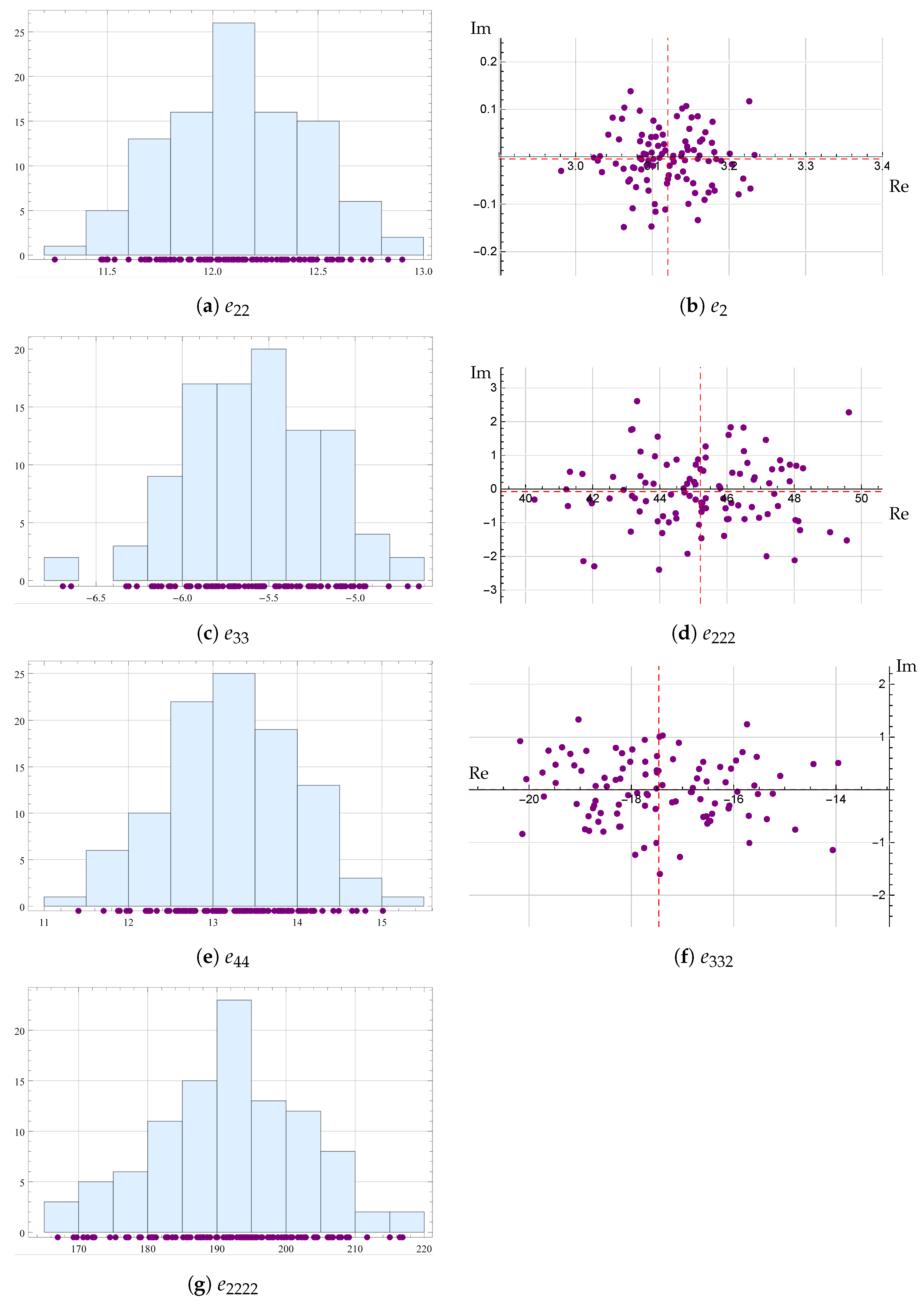The stability of the Formulas (43)–(46) during the simulations is different and depends on f, as shown in

Table 1. Structural sums simulated by RSA for the square array 50 times with $f=0.126$.

Structural Sum	Real Part			Imaginary Part
	Mean	Median	St. Dev.	Mean	Median	St. Dev.
$e_2$	$3.1085$	$3.0754$	$0.3021$	$0.0199$	$0.0016$	$0.3594$
$e_{22}$	$25.5157$	$25.7152$	$2.9871$	0	0	0
$e_{33}$	$-60.2746$	$-58.2463$	$8.7796$	0	0	0
$e_{44}$	$296.702$	$305.671$	$55.7525$	0	0	0
$e_{222}$	$126.848$	$128.309$	$29.7531$	$-0.8130$	$-6.4829$	$27.8381$
$e_{332}$	$-186.629$	$-183.168$	$61.6119$	$4.5258$	$15.9828$	$62.4439$
$e_{2222}$	$1375.21$	$1385.35$	$316.249$	0	0	0

,

Table 2. Structural sum simulated by RSA for the square array 300 times with $f=0.377$.

Structural Sum	Real Part			Imaginary Part
	Mean	Median	St. Dev.	Mean	Median	St. Dev.
$e_2$	$3.1203$	$3.1168$	$0.0496$	$0.0045$	$-0.0032$	$0.0592$
$e_{22}$	$12.1183$	$12.1194$	$0.3369$	0	0	0
$e_{33}$	$-5.5869$	$-5.5707$	$0.4074$	0	0	0
$e_{44}$	$13.2102$	$13.1334$	$0.755$	0	0	0
$e_{222}$	$45.2035$	$45.234$	$1.982$	$-0.0761$	$-0.1515$	$1.0108$
$e_{332}$	$-17.4618$	$-17.5099$	$1.3918$	$0.0066$	$0.0298$	$0.6047$
$e_{2222}$	$191.953$	$192.084$	$11.0702$	0	0	0

and

Table 3. Structural sum simulated by RSA for the hexagonal array 300 times with $f=0.377$.

Structural Sum	Real Part			Imaginary Part
	Mean	Median	St. Dev.	Mean	Median	St. Dev.
$e_2$	$3.1579$	$3.1578$	$0.0593$	$-0.0334$	$-0.0325$	$0.0585$
$e_{22}$	$12.3477$	$12.3267$	$0.4369$	0	0	0
$e_{33}$	$-5.6218$	$-5.5683$	$0.4733$	0	0	0
$e_{44}$	$12.8865$	$12.8756$	$0.771814$	0	0	0
$e_{222}$	$46.46$	$46.3576$	$2.5506$	$-0.5219$	$-0.4534$	$0.9692$
$e_{332}$	$-17.803$	$-17.6024$	$1.6337$	$0.2966$	$0.2465$	$0.6982$
$e_{2222}$	$197.648$	$198.093$	$14.0561$	0	0	0

and Figure 4, Figure 5 and Figure 6. One can see that the shape of cell Q, be it square or hexagonal, practically does not influence the structural sums. The strongest dependence is on the basic concentration of the stable protocol $RSA\left(f\right)$. The $RSA\left(f\right)$ protocol becomes less stable with f decreasing. Thus, the deviation of $e_2$ near $\pi$ for $f=0.126$ as shown in Figure 4 is higher than the deviation of $e_2$ for $f=0.377$ shown in Figure 5b and Figure 6b.

7. Step 3: Applying Padé Approximation to Resummation of Truncated Series

However, a polynomial approximation may not fall within the rigorous bounds, since a polynomial cannot approximate structures in the percolation regime. This yields the final step of renormalization of the truncated series [34].

Considering the iterated root approximants for extrapolation allows us to avoid assuming factorization of the formulas for effective quantities [35]. Let us construct, in the case of RWs, the so-called iterated root approximant:

$$r_4\left(f\right)={\left({\displaystyle \frac{4.11897f^3}{{(0.9069-f)}^3}}+{\left({\left({\displaystyle \frac{1.24116f}{0.9069-f}}+1\right)}^2-{\displaystyle \frac{0.941844f^2}{{(0.9069-f)}^2}}\right)}^{3/2}\right)}^{0.487127},$$

(47)

with the critical index $s\approx 1.46138$. Similar calculations with other polynomial approximations give even worse results.

Since the most direct approach to the construction of the iterated roots does not give satisfactory results, we resort to a more involved strategy of corrected approximations [34,35]. In terms of the variable $z\left(f\right)={\displaystyle \frac{f}{f_c-f}}$, the formula to be corrected is considered in the following form:

$$r_2\left(f\right)={({(1+h_{1}z\left(f\right))}^2+h_{2}z{\left(f\right)}^2)}^{s_0/2},$$

(48)

with the coefficients

$$h_1={\displaystyle \frac{2f_c}{s_0}},h_2={\displaystyle \frac{4(f_c^2-s_0{f}_c)}{s_0^2}},$$

(49)

as we consider below the case of critical index $s_0=1$. The latter condition corresponds to the starting approximation chosen from the self-consistent methods (SCM). The two former formulas are found from the conditions of asymptotic equivalence with the two starting terms in the expansions for $\rho =1$. Let us consider a more general ansatz for the conductivity ${\lambda }_e\left(f\right)$, i.e.,

$${\lambda }_e\left(f\right)=R\left(f\right)={({(1+h_{1}z\left(f\right))}^2+h_{2}z{\left(f\right)}^2)}^{S\left(f\right)/2}.$$

(50)

For the index function $S\left(f\right)$, we found the following formula in the asymptotic regime:

$$S\left(f\right)\simeq {\displaystyle \frac{2log\left({\lambda }_e\left(f\right)\right)}{log\left({\left(\frac{h_{1}f}{f_c-f}+1\right)}^2+\frac{h_2{f}^2}{{(f_c-f)}^2}\right)}},\mathrm{as}f\to 0.$$

(51)

As $f\to 0$, $S\left(f\right)\to s_0=1$; while as $f\to f_c$, $S\left(f\right)\to s$, the sought value of the critical index.

Extrapolation in the case of expansion ${\lambda }_e^{RW}$ is performed by means of the diagonal Padé approximant:

$$S^{RW}\left(f\right)={\displaystyle \frac{1.5124(0.247208+0.174387f+f^2)}{0.373877+0.263744f+f^2}},$$

(52)

so that the sought value of the critical index $s=S^{RW}\left(f_c\right)=1.29357$. For the critical amplitude, directly from the corresponding approximation for $R\left(f\right)$, one can find $B\approx B^{RW}=1.77492$.

Extrapolation in the case of expansion ${\mathit{\lambda }}_e^{RSA}$ is performed similarly to the former case, with the index function

$$S^{RSA}\left(f\right)={\displaystyle \frac{1.45365(0.238741+0.121243f+f^2)}{0.347046+0.176245f+f^2}},$$

(53)

and the sought value of the critical index $s=S^{RSA}\left(f_c\right)=1.28067$. For the critical amplitude, we find $B\approx B^{RSA}=1.76479$.

Extrapolation in the case of expansion ${\lambda }_{sq}^{RSA}\left(0.377\right)$ by means of the non-diagonal Padé approximant $p_{2,4}$, with the index function

$$S_{sq}^{RSA}\left(f\right)={\displaystyle \frac{4.0066(0.159162+0.230569f+f^2)}{(1.96663-f)(2.1175+f)(0.153134+0.227384f+f^2)}},$$

(54)

and the sought value of the critical index $s=S_{sq}^{RSA}\left(f_c\right)=1.25953$. For the critical amplitude, we find $B\approx B_{sq}^{RSA}=1.74832$.

Extrapolation in the case of expansion ${\lambda }_{hex}^{RSA}\left(0.377\right)$ by means of the non-diagonal Padé approximant $p_{2,4}$, with the index function

$$S_{hex}^{RSA}\left(f\right)={\displaystyle \frac{4.0686(0.159592+0.227793f+f^2)}{(1.97768-f)(2.13806+f)(0.153561+0.22501f+f^2)}},$$

(55)

and the sought value of the critical index $s=S_{hex}^{RSA}\left(f_c\right)=1.2569$. For the critical amplitude, we find $B\approx B_{hex}^{RSA}=1.74628$.

All our current estimates for the critical amplitudes are close to each other, i.e., are weakly dependent on protocols. Various formulas for the effective conductivity obtained by the RW simulations are presented in Figure 7.

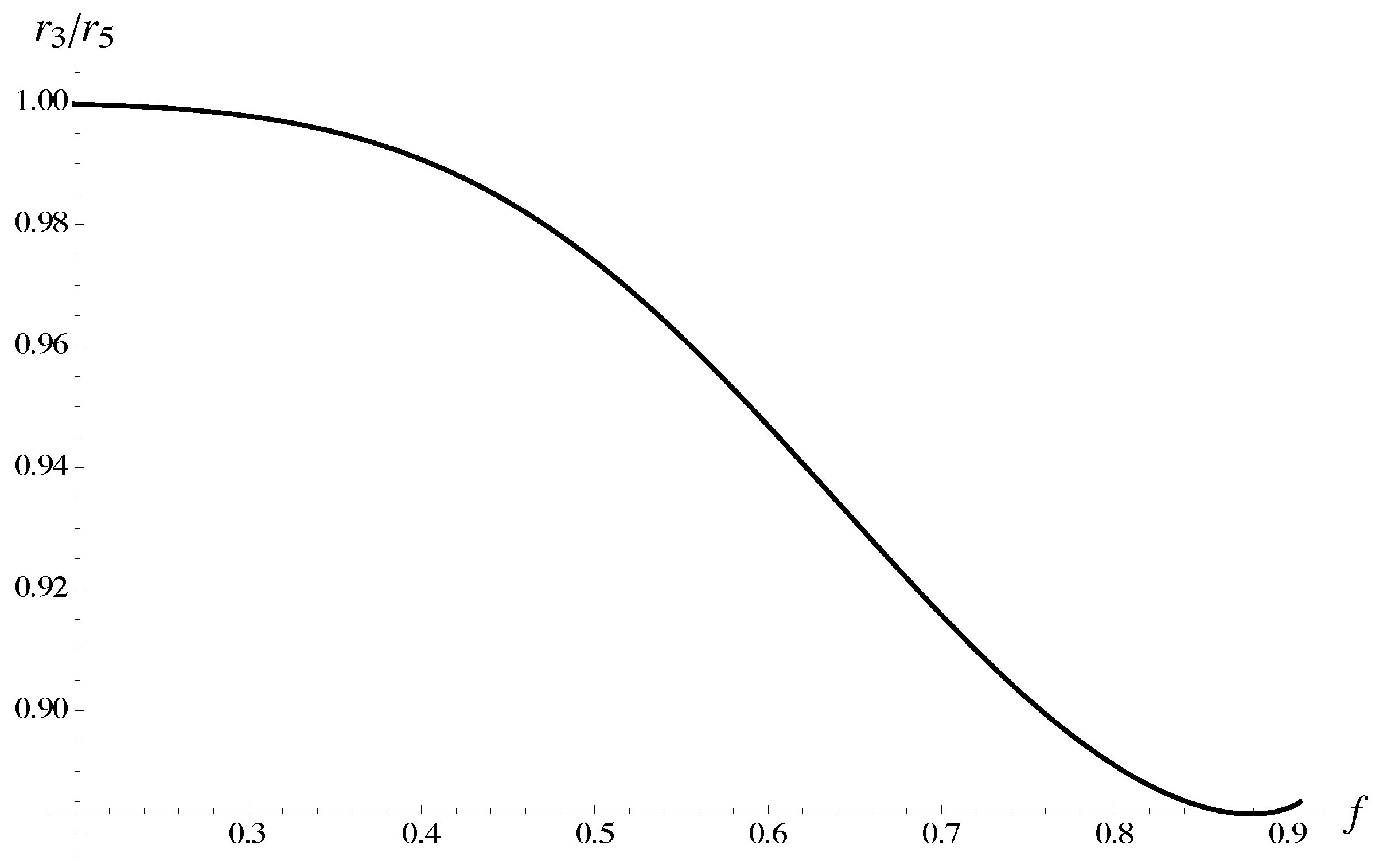
Remark 2. 

If we consider a different, factorized expression for the effective conductivity developed in [35],

$${\lambda }_e\left(f\right)=F\left(f\right)={(1+g_{1}f)}^{c_1}{(1-f/f_c)}^{C\left(f\right)},$$

where $g_1=\left(f_c{(2f_c-1)}^{-1}\right)$, $c_1={(2f_c-1)}^2$, then the index function $C\left(f\right)$ has the following form for $f\to 0$:

$$C\left(f\right)={\displaystyle \frac{log\left({\lambda }_e\left(f\right){(1+g_{1}f)}^{-c_1}\right)}{log(1-f/fc)}},$$

and $C\left(0\right)=-1$. Extrapolating the index function to $f\to f_c$ in the case of expansion ${\lambda }_{hex}^{RSA}\left(0.377\right)$ by means of the non-diagonal approximant $p_{4,2}$ brings $s=1.32605$ and $B\approx 1.49362$. Similarly, for ${\lambda }_{sq}^{RSA}\left(0.377\right)$, we compute $s=1.32842$ and $B\approx 1.49327$. However, the results for ${\lambda }_e^{RW}$ and ${\lambda }_e^{RSA}$ are not better than for simple iterated root approximants.

Remark 3. 

Sometimes, in addition to the critical index, one would like to estimate the so-called correction-to-scaling indices [35]. Relevant self-similar root approximants [34,35], with $s=1.3$, and coefficients are found from asymptotic equivalence with ${\lambda }_{hex}^{RSA}$:

$$r_3\left(f\right)={\left({\displaystyle \frac{3.0669f^3}{{(0.9069-f)}^3}}+{\left({\displaystyle \frac{9.16243f^2}{{(0.9069-f)}^2}}+{\left({\displaystyle \frac{5.45029f}{0.9069-f}}+\right)}^{0.974461}\right)}^{0.788102}\right)}^{0.433333},$$

gives the correction-to-scaling critical index $s_1=-1.4238$, so that in the vicinity of $f_c$,

$$r_3\left(f\right)\propto z{\left(f\right)}^{1.3}(1+O\left(z{\left(f\right)}^{s_1}\right).$$

For comparison, let us construct also the iterated root approximant based on the same input as $r_3\left(f\right)$,

$$r_5\left(f\right)={({({({({(1+h_{1}z\left(f\right))}^2+h_{2}z{\left(f\right)}^2)}^{3/2}+h_{3}z{\left(f\right)}^3)}^{4/3}+h_{4}z{\left(f\right)}^4)}^{5/4}+h_{5}z{\left(f\right)}^5)}^{s/5},$$

with $h_1=1.39523$, $h_2=-0.843793$, $h_3=-0.085794$, $h_4=1.900808$, and $h_5=6.411259$. The ratio $r_3\left(f\right)/r_5\left(f\right)$ is shown in Figure 8.

8. Conclusions

This paper bridges the gap between theory and concrete applications of the concept of randomness. We focus on the effective properties of 2D conducting random composites with circular inclusions distributed without overlaps. In particular, we encountered a diversity of random composite materials within this class. In particular, we conclude that there is no universal minimum number of inclusions per cell in simulations of random composites. Even seemingly slight modifications to RSA algorithms result in different formulas for the effective constants.

Applying the aRVE theory methodologically and practically addresses the diversity problem of random composites based on homogenization principles. This paper develops the investigation strategy and provides a constructive description of each step. The aRVE theory precisely answers the question of how a spatial arrangement of inclusions within similar-in-spirit protocols influences the overall effective properties of the composites.

Only proper protocols for random structure generation result in stable effective properties. For instance, the effective conductivity was found by the RSA and RW protocols for all admissible concentrations. The latter methods were designed specifically for simulations of uniform distributions of perfectly conducting particles. The results given by Equations (39) and (40) practically coincide, including the critical index $s=1.3$. It is also observed that the results are weakly dependent on the unit cell Q. The hexagonal and square shapes of Q were considered above.

However, if we slightly change the parameters of the protocols, the results may change essentially. This is the main result of the present paper. Therefore, there is no such thing as the most appropriate protocol in practice. This observation was also confirmed in [36], where nine different types of interactions between particles were investigated. The particles might be attracted, repulsed, or neutral to each other. The particles might form various clusters. Our observations are also confirmed by recent studies of metamaterials with exceptional geometries. The properties of such metamaterials appear to be exceptionally different from the properties of other similar geometries.

It is even possible to get an idea about the accuracy of the theory for the effective quantities at moderate concentrations. In the book [34], several examples of such computations are provided. Typically, the estimates of the effective constants closely match the simulations, with a percentage error of much less than 1%. However, if the protocol involves an increase in the probability of higher percolation chains, the error may become significant.