Balancing Depth for Robustness: A Study on Reincarnating Reinforcement Learning Models

Abstract

This paper investigates the impact of adaptive network depth selection on the robustness and performance of Regenerative Reinforcement Learning (RRL) models. RRL accelerates learning by reusing previously computed results. We propose a task-driven approach to dynamically configure network depth to explore the best architecture on Atari 2600 games. The experimental results show that a seven-layer network achieves the best balance between feature extraction, policy learning, and robustness, achieving an IQM score of 1.2 in a pool of 10 games. While deeper networks risk overfitting, shallower architectures struggle to cope with complex task dynamics. Our results highlight the key role of adaptive depth in enhancing the generalization, stability, and efficiency of RRL models.

1. Introduction

Reinforcement learning (RL) is an important machine learning method that uses intelligent agents to learn strategies to maximize cumulative rewards through trial and error in an environment [1]. However, traditional RL methods often rely on table lookup or simple function approximation, which is not scalable enough in high-dimensional and complex tasks. To address this problem, deep reinforcement learning (DRL) uses deep neural networks to process complex states [2], which significantly improves performance, but its training process is still resource-intensive and difficult to achieve effective knowledge transfer. To solve this problem, Agarwal et al. formally proposed a research paradigm called recurrent reinforcement learning (RRL), which aims to accelerate the new learning process by reusing existing computational results and training experience [3].

Reincarnating reinforcement learning has similarities with traditional transfer learning [4] and meta-learning [5], but its uniqueness lies in its focus on how to effectively utilize the computational results of previous models so that they can quickly adapt and continue to optimize when faced with new tasks. This method is particularly suitable for use in resource-constrained environments and can significantly reduce the computational cost of retraining models [6]. Therefore, exploring how to further improve the performance and robustness of the model in RRL has become an important direction of current research. In reinforcement learning models, deep neural networks (DNNs) play a core role as approximators of policy and value functions [7]. The structural design of deep neural networks, especially the depth of the network, directly affects the performance of the model. Traditional research shows that increasing the depth of the network can improve the expressiveness of the model and enable the model to fit more complex functions [8]. However, excessive network expansion may also lead to overfitting problems and reduce the generalization ability of the model. The dropout technique can effectively prevent overfitting of deep networks [9].

The exploration of the robustness of Reinforcement Learning (RL) networks has garnered significant interest, driven by the urgent need for agents to reliably perform under various conditions [10]. The influence of different neural network depths has been studied from the perspective of the universal approximation theorem [11,12], as well as functional expressivity [13]. Research on the hierarchical training of deep linear networks based on Block Coordinate Gradient Descent (BCGD) has also been conducted, with convergence analyses establishing optimal learning rates and examining the effects of depth and initialization on training [14].

In addition, studies have found that the skip connection operation used in WRN can improve the robustness of deeper architectures [15]. On the other hand, there have also been studies showing that increasing the number of parameters of the same type of deep neural network architecture can only lead to limited robustness improvements [16,17]; wider networks may lead to more perturbation instabilities [18].

The impact of network depth on the robustness of trained DNNs challenges the belief that more parameters always enhance robustness, indicating the existence of an optimal configuration for adversarial robustness [19]. Investigations into how variations in network depth influence hidden representations have revealed block structures in large models that emerge due to over-parameterization relative to the training set size [20].

Previous empirical work has examined the effects of width and depth on model accuracy in the context of Convolutional Neural Network (CNN) architecture design, finding that optimal accuracy is often achieved by balancing width and depth [21,22]. Further study of accuracy and error sets has been conducted in [23] (error sets over training) and [24] (error after pruning). Other work has demonstrated that it is often possible for narrower or shallower neural networks to attain similar accuracy to larger networks when the smaller networks are trained to mimic the larger networks’ predictions [25,26]. We instead seek to study the impact of width and depth on network internal representations and (per-example) outputs by applying techniques for measuring the similarity of neural network hidden representations [27,28,29]. These techniques have been very successful in analyzing deep learning, from the properties of neural network training [30,31], objectives [32], and dynamics [33] to revealing the hidden linguistic structure in large language models [34,35] and applications in neuroscience [36] and medicine [37].

Although a large number of studies have shown that network depth has a significant impact on model performance, the role of network depth has not been fully explored in the special field of RRL. Under a limited sample budget, whether the student agent can fully extract task-critical features is closely related to the network depth design, which puts higher requirements on the optimization of RRL models. To address this issue, this study aims to systematically analyze the impact of different network depths on the performance and robustness of RRL models. We explore how changes in network structure affect the performance of the model under different task environments. Through comparative experiments, we hope to provide empirical evidence for optimizing the network structure of regenerative reinforcement learning models, thereby improving the generalization ability and robustness of the model in practical applications.

2. Materials and Methods

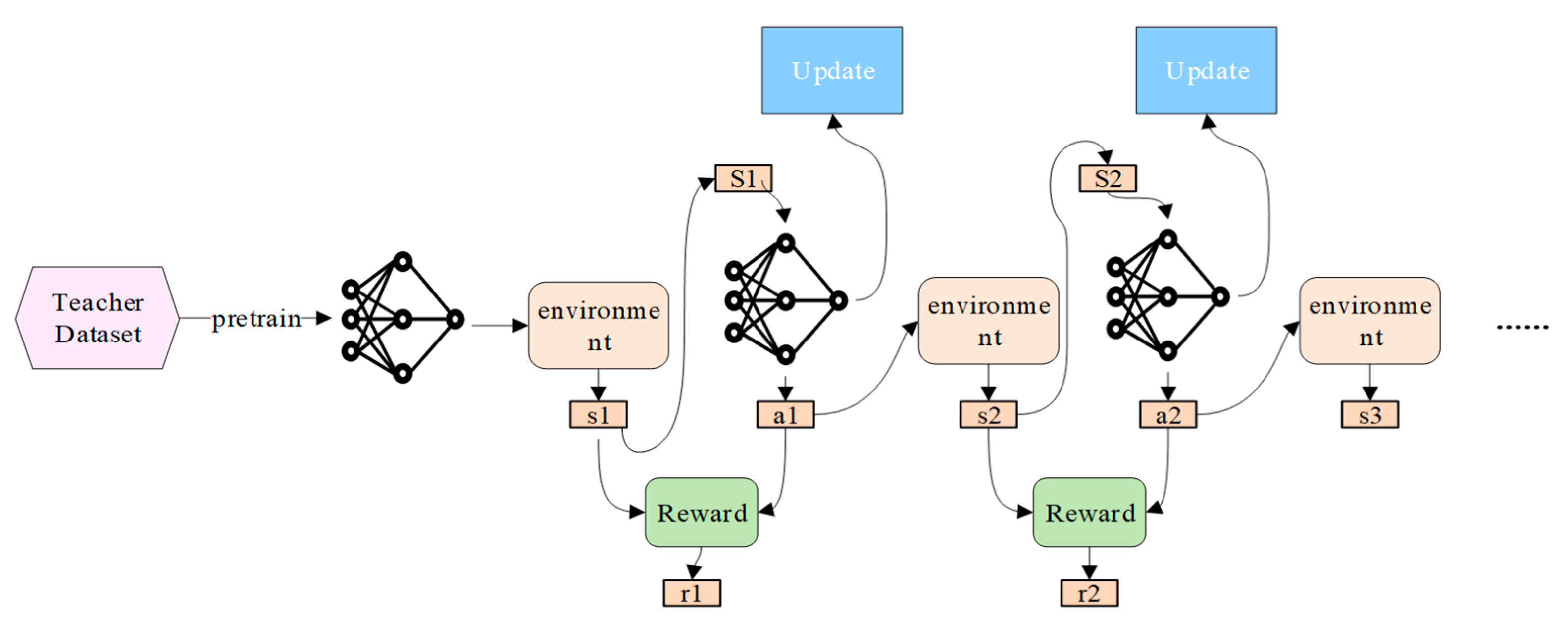
Reinforcement Learning (RL) is a machine learning paradigm that learns how to make decisions by interacting with an environment. In RL, an agent performs actions to influence the environment, receives rewards, and improves its behavior strategy based on these feedbacks to maximize the cumulative rewards. Most RL research is based on the absence of prior knowledge, but large-scale RL systems usually need to run for a very long time and constantly interact with new data. Starting them from scratch will take weeks or even months, which makes methods that do not exploit prior knowledge inefficient. For example, a system that plays Dota 2 like a human underwent months of RL training during its development and constantly changed (e.g., model architecture, environment, etc.), which required building on previously trained systems to avoid retraining from scratch.

Deep Q-Network (DQN) is a DRL technique that approximates Q-values using neural networks instead of Q-tables. Q-values are computed using the Bellman equation [38], as shown in Equation (1):

$$Q(s,a)=r+\gamma \underset{a}{max} Q(s^{\prime },a^{\prime })$$

(1)

where $\gamma$ is the discount factor controlling the weight of the next state, with values between 0 and 1. $Q\left(s,a\right)$ represents the value of taking action a in state $s$, $r$ is the immediate reward received after executing action a in state s, $s^{\prime }$ is the new state reached, and $a^{\prime }$ represents all possible actions in state s′.

The concept of reincarnating RL addresses the need to quickly iterate on a problem or test new strategies without restarting from scratch, as depicted in Figure 1.

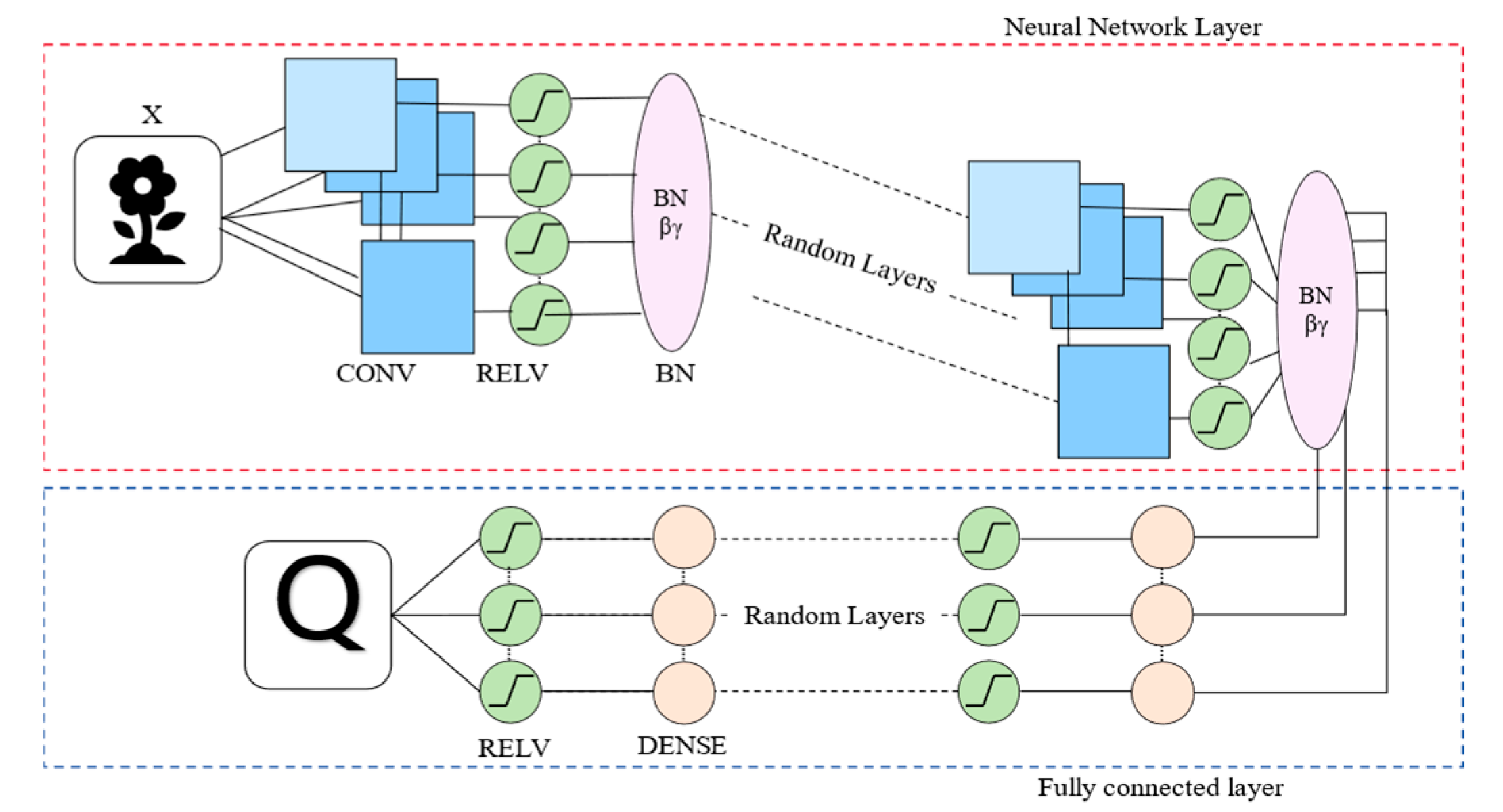
This paper presents an adaptive deep Q-Dagger network architecture based on RRL (Figure 2), which aims to improve model robustness and generalization ability by dynamically adjusting the network depth configuration. Unlike traditional RL models with fixed network depth, our method customizes the network depth according to task complexity and explores the best architecture to enhance multi-task performance flexibility. Task complexity can be calculated by the following indicators:

$$C_{task}=w_1\mathrm{S}+w_2\mathrm{R}+w_3\mathrm{A}$$

(2)

Among them, $w_1$, $w_2$, and $w_3$ are weight coefficients used to reflect the impact of different task characteristics on complexity. $\mathrm{S}$ is the state space dimension, $\mathrm{R}$ is the reward sparsity, and $\mathrm{A}$ is the action space dimension.

Adaptive Network Design: RRL seeks to reduce training time and computational resource usage by reusing previous results and training experiences. However, the network’s structural design—particularly its depth—plays a crucial role in determining learning outcomes and model stability. To address this, this study introduce a depth-adaptive Q-Dagger network capable of adjusting its architecture according to task complexity, with the following key design steps:

(1)

Network Parameter Initialization: Network weights are initialized using the Xavier uniform distribution to maintain training stability.

(2)

Convolutional Layer Generation: The number of convolutional layers is adaptively chosen based on task complexity, ranging from 1 to 5 layers. The number of filters per layer is randomly selected from {32, 64, 128, 256}, with a fixed kernel size of 3 × 3 and a stride of 1 × 1. ReLU activation and batch normalization are applied to enhance stability and improve learning dynamics.

(3)

Fully Connected Layer Generation: The number of fully connected layers is adaptively selected between 1 to 3 layers, with the number of neurons per layer randomly chosen from {64, 128, 256}. ReLU activation is applied to increase the network’s non-linear representation capacity.

(4)

Output and Feature Representation Layers: Finally, a feature representation layer outputs a 128-dimensional feature vector, which effectively connects to the output layer to generate the final Q-values, guiding the agent’s decisions in the reinforcement learning environment.

This study constructs models with varying depths by incrementally increasing network depth d while maintaining other parameters unchanged, thereby isolating depth as the primary factor affecting performance. The network output $Q_d(s,a)$ is expressed as:

$$Q_d(s,a)=f_d(s,a;\theta )$$

(3)

where $f_d$ is a neural network function with depth $d$, and $\theta$ represents model parameters.

The network depth directly affects the expressiveness and robustness of the model. Appropriately increasing the depth can enhance the feature extraction ability of the model, but a network that is too deep may lead to overfitting and unstable training. Therefore, the impact of network depth on model robustness is a key factor. According to the Universal Approximation Theorem, any continuous function can be approximated by a sufficiently deep neural network. However, the approximation ability alone cannot fully explain the effect of deep networks in actual tasks, especially when the complexity of the task and the uncertainty of the environment increase; the performance of deep networks may decrease due to overfitting. In order to better understand the impact of network depth on robustness, we consider the following model of depth and performance:

$$f_L\left(x\right)={\sum }_{i=1}^{N_L} {\alpha }_i\sigma (W_{L}x+b_L)$$

(4)

Among them, $f_L\left(x\right)$ represents the output of a neural network with a depth of $L$, $N_L$ is the number of neurons in the Lth layer of the network, and $W_L$ and $b_L$ are the weight and bias of the layer, respectively. A deeper network can represent a more complex mapping, but the higher the complexity, the easier it is to capture noise during training. This can be reflected in the following mathematical model:

$$E_{gen}\left(L\right)=E_{bias}\left(L\right)+E_{variance}\left(L\right)+E_{complexity}\left(L\right)$$

(5)

Expression error $E_{bias}\left(L\right)$: As the depth $L$ increases, the representation ability of the network improves, and the expression error decreases. Variance error $E_{variance}\left(L\right)$: When the depth is too large, the network may begin to fit the noise in the training data, the variance increases, and overfitting occurs. Complexity error $E_{complexity}\left(L\right)$: When the depth is too large, the network complexity is too high, which may also lead to a decrease in the generalization ability on the test data.

In order to quantify the impact of network depth on generalization ability, this study introduced the Rademacher Complexity model [39,40]. Rademacher complexity measures the sensitivity of the network structure to random noise and reflects the complexity and robustness of the model. Let the network model be $f_{\theta }\left(x\right)$ where $x$ is the input, $\theta$ is the network parameter, $\mathrm{S}$ = {$x1$,$x2$,$\dots$,$xn$} is the training data set, and the Rademacher complexity of the network is:

$${\mathcal{R}}_n\left(f\right)=\mathbb{E}\left[\underset{\theta }{sup} {\displaystyle \frac{1}{n}}{\sum }_{i=1}^n \sigma \left(f_{\theta }\left(x_i\right)\right)\right]$$

(6)

where $\sigma$ is the activation function and E represents the expectation for all input data. According to this formula, as the network depth increases, the Rademacher complexity increases, which means that the network may be more sensitive to noise in the training data, leading to overfitting. However, within a reasonable range of network depth, the Rademacher complexity increases with depth until it reaches a balance point. This also explains why a network depth of seven layers may be at the optimal balance point between generalization ability and noise sensitivity.

Feature Extraction Ability and Depth: The network depth $d$ is closely related to the model’s feature extraction capability. For an input $X$, the output of the depth d layer can be represented as:

$$Z_d=W_d\cdot f_{d-1}\left(X\right)+b_d$$

(7)

Here, $W_d$ and $b_d$ denote the weight matrix and bias vector of the depth d layer, respectively, and $f_{d-1}\left(X\right)$ represents the output of the depth d layer.

To evaluate the robustness of different network depths against perturbations, we define the robustness loss $L_{robust}$ as:

$$L_{robust}\left(d\right)={\mathbb{E}}_{\delta }\left[\parallel Q_d(s+\delta ,a)-Q_d(s,a){\parallel }^2\right]$$

(8)

This loss function measures the extent of changes in the network’s output before and after input perturbations. Higher robustness should correspond to a smaller $L_{robust}\left(d\right)$.

This loss function measures the change in network output before and after input perturbation, with lower values indicating higher robustness. The total evaluation combines task loss $L_{Qdagger}\left(d\right)$ and robustness loss: where $\lambda$ is a weighting parameter balancing task performance and robustness.

$$L_{total}\left(d\right)=L_{Qdagger}\left(d\right)+\lambda \cdot L_{robust}\left(d\right)$$

(9)

This architecture allows automatic depth optimization tailored to specific task environments, achieving a balance between feature extraction and training efficiency.

Many studies have explored the impact of network depth on model performance. Generally speaking, deeper networks can represent more complex functional relationships. However, how to strike a balance between different depths to optimize the robustness of the model remains an open question. Especially in the context of regenerative reinforcement learning, different network structures may have different effects on the performance of the model, so it is of great research value to deeply explore the relationship between network structure and model robustness.

In addition, regenerative reinforcement learning also faces the challenge of how to effectively utilize historical models. According to the research of Agarwal et al., RRL can not only accelerate the learning of new tasks by reusing calculation results but also cope with the uncertainty in task changes by adjusting the model architecture. Therefore, the design of the network structure is particularly important in RRL. It not only affects the learning speed and performance of the model but also plays a key role in the robustness of the model when facing complex environments.

To investigate the impact of network depth, this study designed several sets of regenerative neural networks (Q-Dagger) with different depths, which are adaptively selected based on task complexity. This approach allows us to explore how different network depths tailored to each task affect model performance. The Algorithm 1 outlines the methods used in our study.

Algorithm 1: Adaptive Deep Network Architecture for Reinforcement Learning.

Initialization: Use Xavier uniform initializer for network parameters. Preprocess Input: If inputs_preprocessed is False, preprocess input x. Convolutional Layers: Adaptively choose conv_layers (1–5) based on task complexity (state space size, reward sparsity, action space size). For each layer, randomly select features from {32, 64, 128, 256}, and use (3, 3) kernel, (1, 1) strides. Apply convolution, ReLU, and BatchNorm. Flatten: Reshape the output tensor to prepare for fully connected layers. Fully Connected Layers: Adaptively choose fc layers (1–3) based on task complexity and training feedback. For each layer (except last), randomly select units from {64, 128, 256}, apply dense and ReLU. Representation Layer: Add a dense layer with 128 units, apply ReLU. Output Layer: Add a dense layer to produce num_actions Q-values. Return: Return Q-values and representation.

To evaluate the performance of networks of different depths in regenerative reinforcement learning (RRL), this study developed a systematic experimental framework covering several classical reinforcement learning environments. The experiments adopted a controlled variable approach to ensure that the observed performance differences mainly come from the adjustment of network depth. The network depth of each task is selected based on its complexity, including factors such as state space size, reward sparsity, and action space size, and then we add slightly higher or lower network depths for comparison. The experimental design includes the following steps:

(1)

Environment Selection: This study selected classic reinforcement learning environments, such as Atari 2600, which exhibit high levels of dynamics and uncertainty, to effectively assess the impact of different depths on model performance.

(2)

Training Setup: All networks were trained under identical settings, including the number of training steps, the learning rate, and the optimizer (Adam), to ensure comparability across different depths. To mitigate the impact of randomness on experimental results, each network configuration was tested multiple times, and the results were averaged.

(3)

Robustness Testing: After training in standard environments, this study conducted additional robustness tests on networks of different depths, including introducing external perturbations, such as image blurring, to evaluate the impact of depth on the ability to withstand disturbances. These tests help us better understand the relationship between network depth and robustness.

3. Results

The experiments were conducted in a variety of classic reinforcement learning environments, including but not limited to Atari games and MuJoCo simulation tasks. These environments were selected because they provide rich dynamics and uncertainty, which helps to fully test the impact of network structure on RRL models. In each experimental environment, we used the established standard settings while introducing additional noise or perturbation factors to evaluate the robustness of the model. For example, in Atari games, we may adjust the clarity of the input image.

This section presents the experimental results and analyzes the impact of network depth on model robustness. We explore how different network structures perform under uncertainty and how adjusting network architecture can enhance model stability. We conducted experiments with ALE with sticky actions. To reduce computational costs, we used a subset of ten common Atari 2600 games: Asterix, Breakout, Space Invaders, Seaquest, Q*Bert, Beam Rider, Enduro, Ms. Pac-Man, Bowling, and River Raid. The related code runs on Ubuntu, using Python 3.10 and TensorFlow-GPU 2.10.

3.1. Performance Exploration of Different Depths

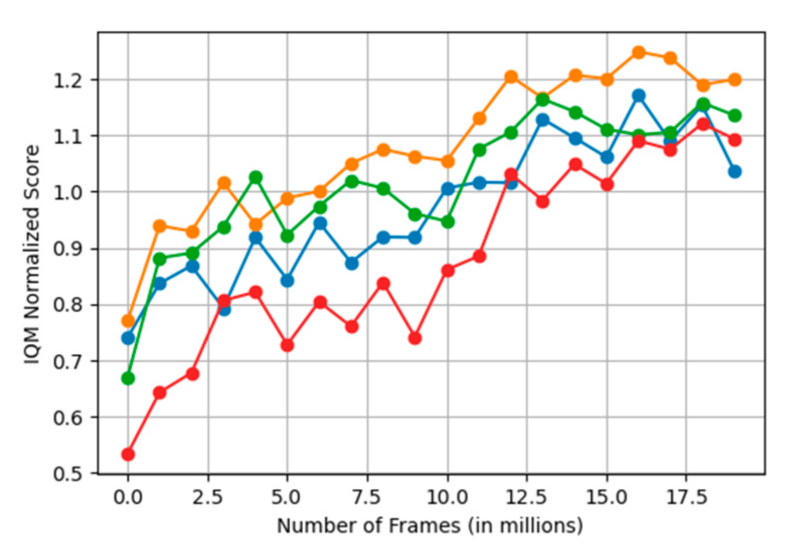
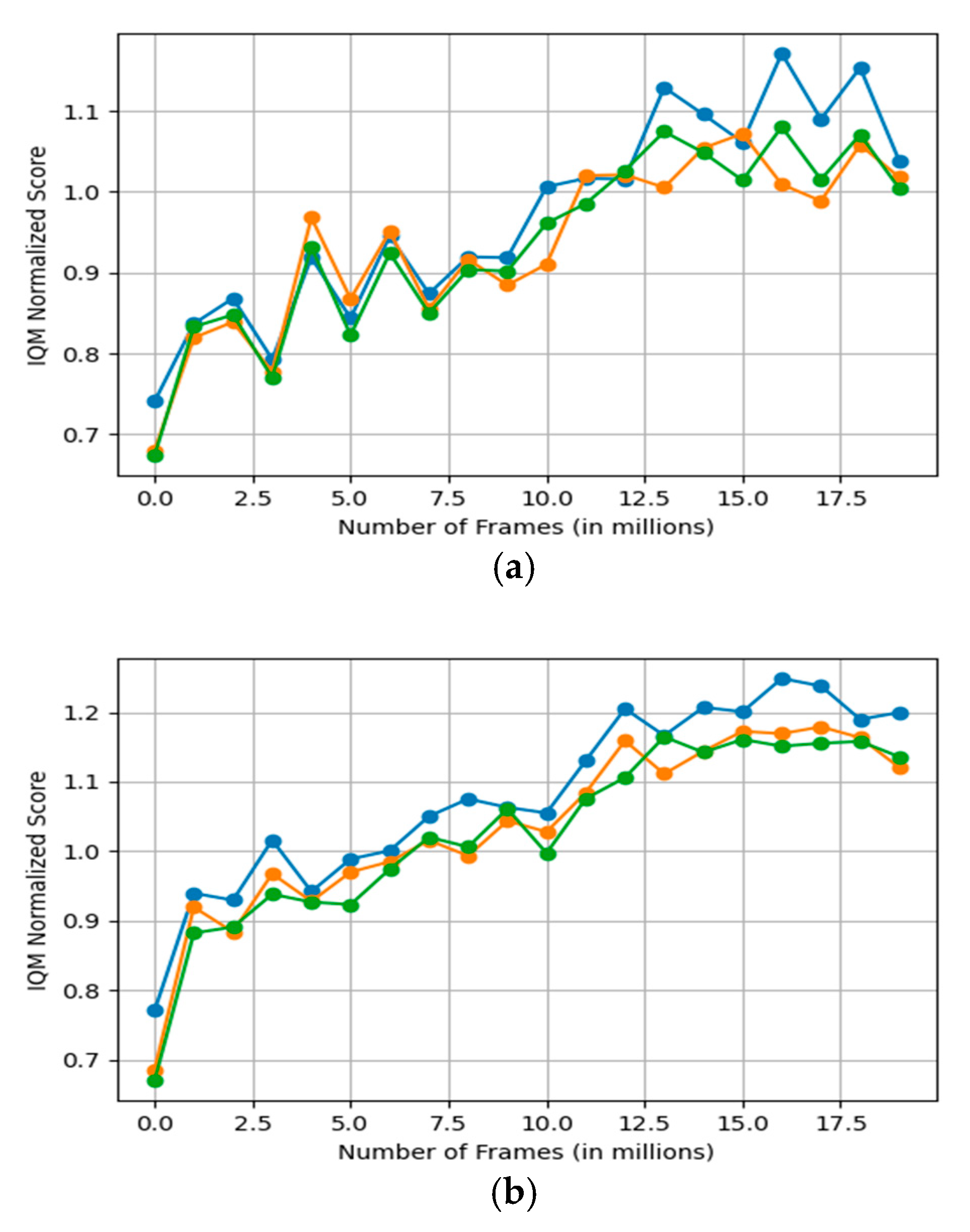
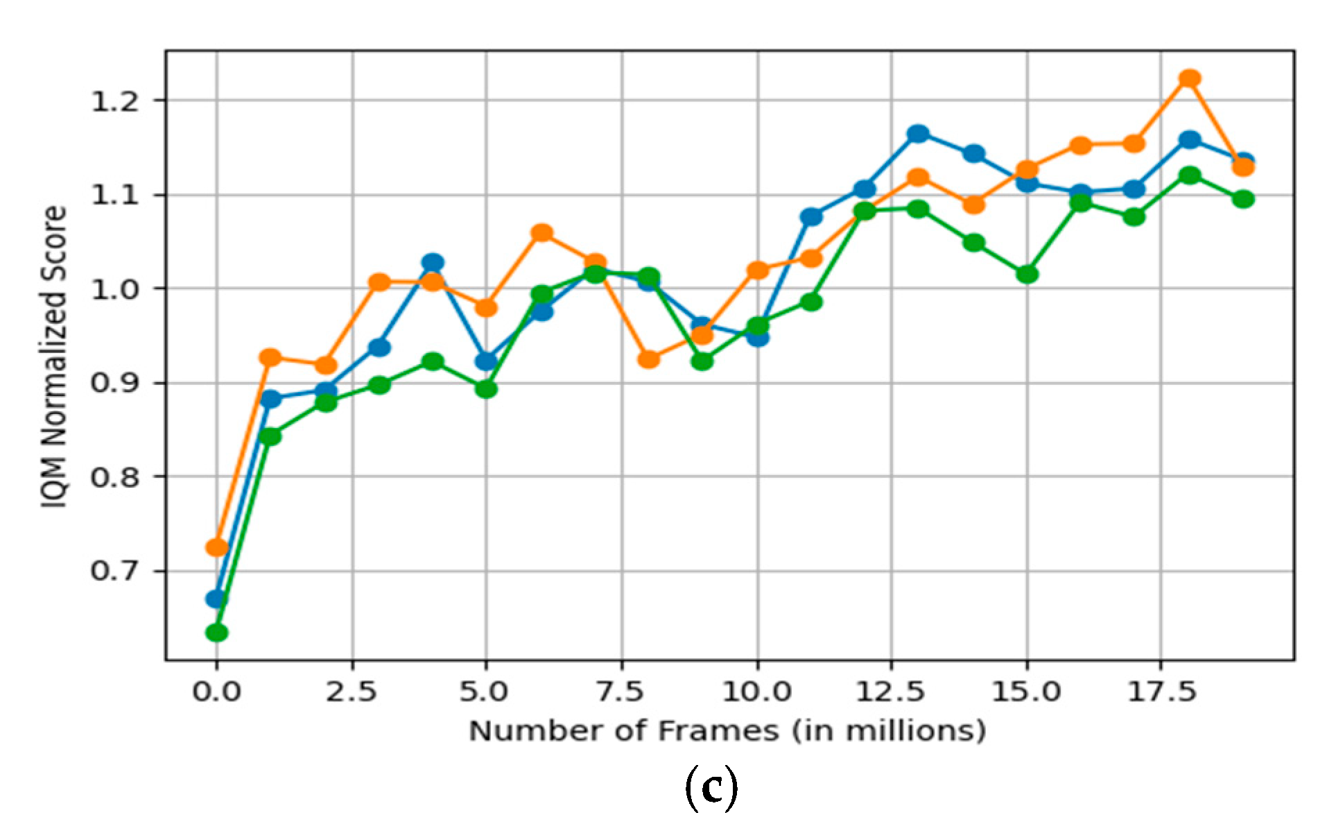
Figure 3 shows the performance of neural networks of varying depths on Atari 2600 games. The y-axis represents the normalized IQM score, while the x-axis represents the number of frames (in millions) in which the agent interacts with the game environment. To evaluate the reproducibility of sample efficiency, the student agent is trained using only 10 million frames—40 times less than the sample budget of the teacher—and the teacher’s help is limited to the first 6 million frames. Here, the first 10 million frames correspond to offline training, and the subsequent 10 million frames correspond to online training. Notably, the seven-layer network (yellow line, containing four convolutional layers and three fully connected layers) consistently achieves the highest IQM scores, especially in the later training stages, indicating that it achieves the best balance between feature extraction and policy learning. In contrast, both shallower (six layers in blue) and deeper (eight layers in green) networks show poor performance. The figure emphasizes the important impact of task complexity on the choice of network depth and highlights the benefits of adaptively tailored architectures.

Are student agents with deeper neural networks also more suitable for regenerative reinforcement learning? In Figure 1, we deny this question. It can be seen that the neural network with a depth of 7 performs better than the networks with depths of 6 and 8 in both offline and online training stages. The network with a depth of 8 is slightly better than the network with a depth of 6. The network with a depth of 6 is not as good as the network with a depth of 7. We speculate that this is because the network still needs enough feature extraction and ability to train, which may not be enough to capture complex patterns in the data. Although deeper networks (such as a depth of 8) can theoretically learn more complex features, they may introduce the risk of overfitting or increase the difficulty of training.

Next, we analyzed the performance of student agents with varying depths in different gaming environments.

For complex shooter games like Space Invaders (Figure 4), the seven-layer network performs best. The eight-layer network can achieve high score peaks in some periods, but when the environment changes significantly or quickly, its score will drop sharply, and even fall below the teacher strategy, showing obvious fluctuations. When the six-layer network faces more complex scenarios, the score is always a bit lagging, indicating that its expressive ability is insufficient.

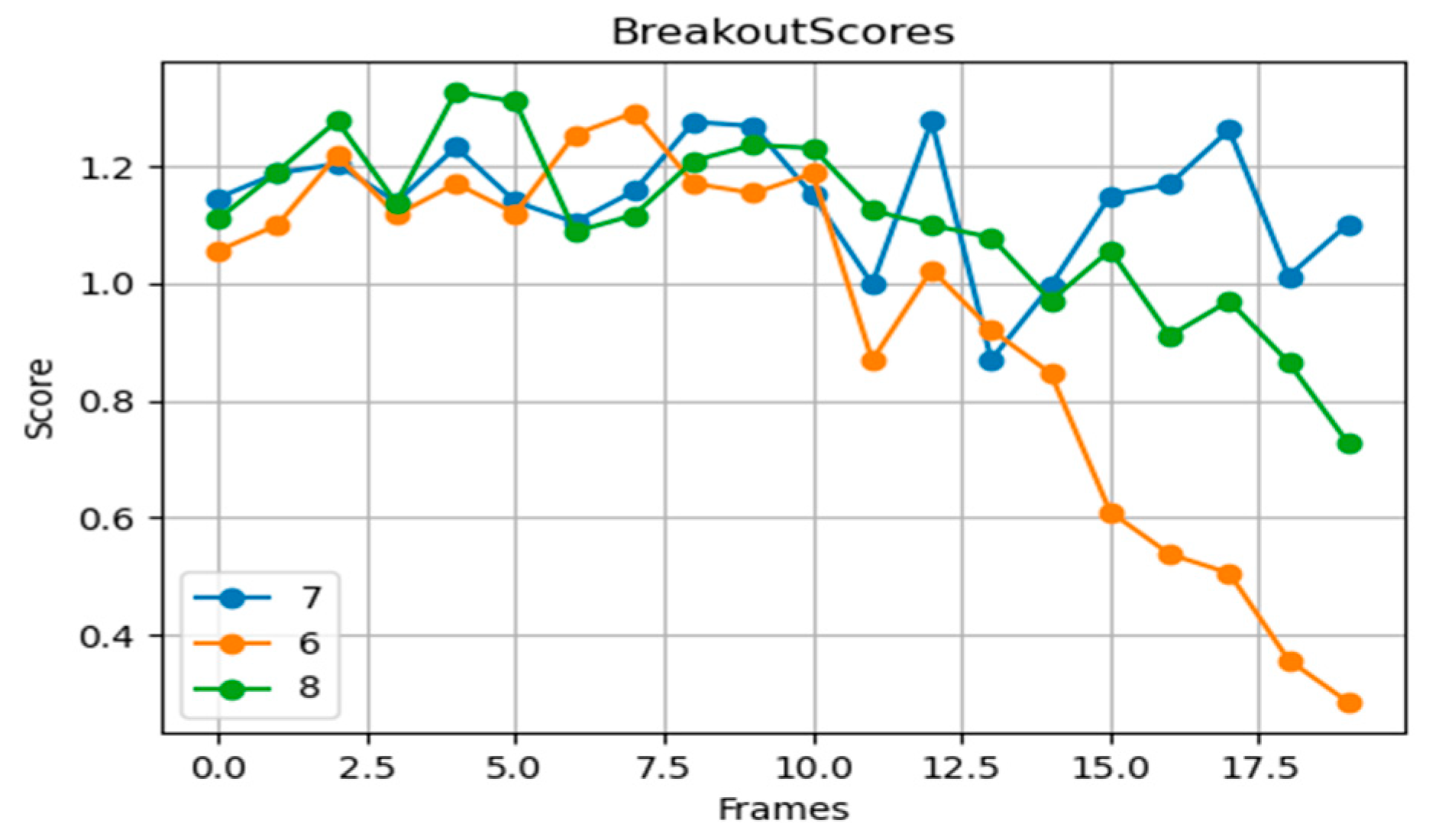
Breakout is a game with simple rules but requires precise control (Figure 5). The seven-layer network exhibits the best score stability, particularly in online training, adjusting strategies quickly. The six-layer network shows slight deficiencies, mainly in responding to random disturbances, while the eight-layer network, despite having a more complex feature extraction capability, may exhibit slower or unstable learning due to its excessive depth.

In Asterix (Figure 6), the seven-layer network excels, particularly in the later training stages, outperforming other network depths. This indicates that the seven-layer depth provides superior feature extraction and strategy learning capabilities for multi-objective and random element environments.

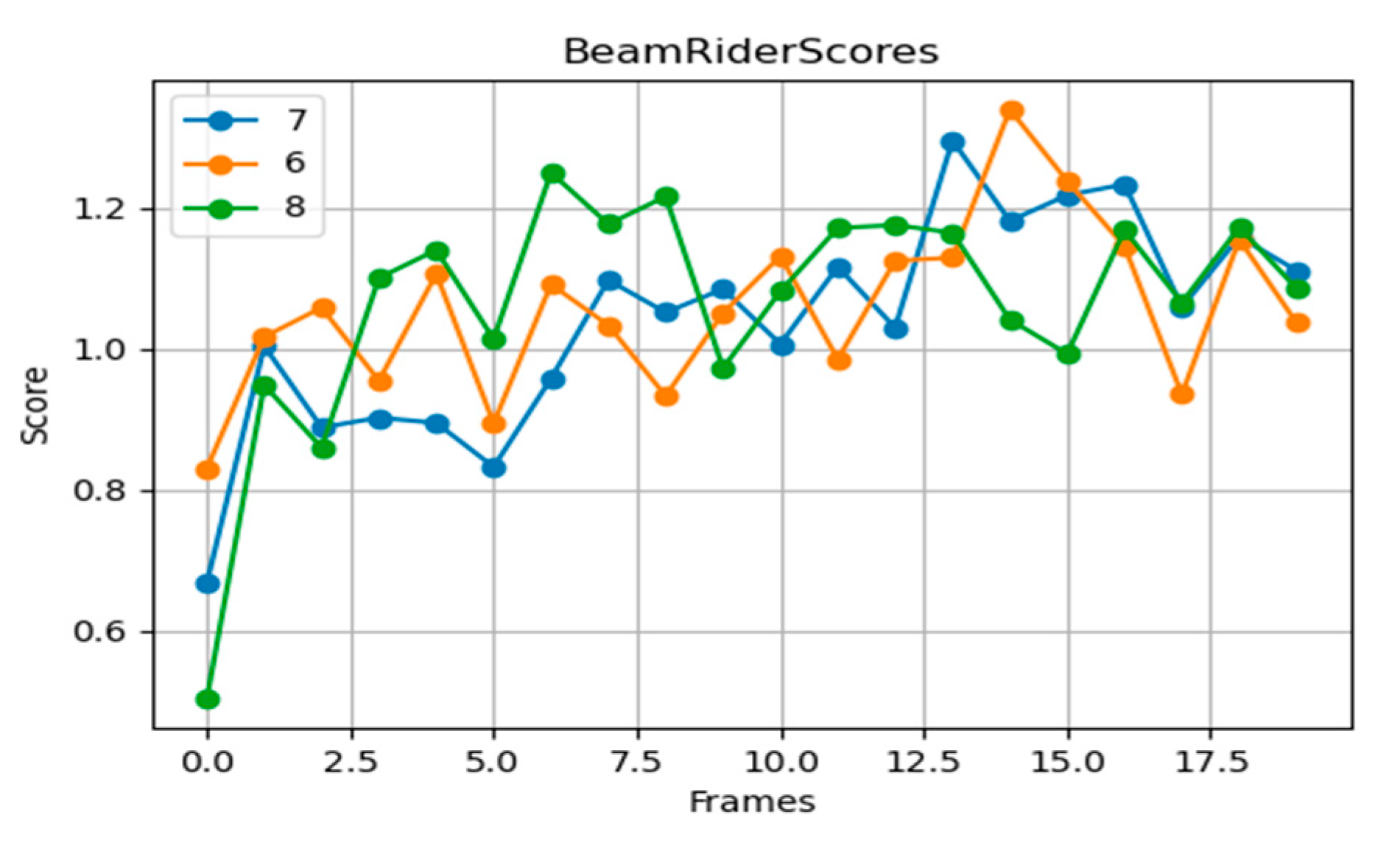
Beam Rider is a game requiring rapid response and continuous shooting (Figure 7), demanding high strategy adjustment and reaction speed. The seven-layer network initially performs steadily, gradually improving its score and surpassing other depths in later stages. In contrast, the six-layer network shows early advantages but struggles to maintain score growth, reflecting slower convergence. The eight-layer network, with its overly deep structure, underperforms in later stages, suggesting learning difficulties or strategy instability.

Throughout most training stages, the seven-layer network maintains the highest scores, demonstrating better performance and robustness in Seaquest (Figure 8). The eight-layer network starts to approach the seven-layer performance in the later training stages (around 10 million frames), but overall scores remain slightly lower. The six-layer network shows slow score improvements, consistently scoring the lowest, indicating that the shallow depth hampers the network’s ability to capture complex dynamics.

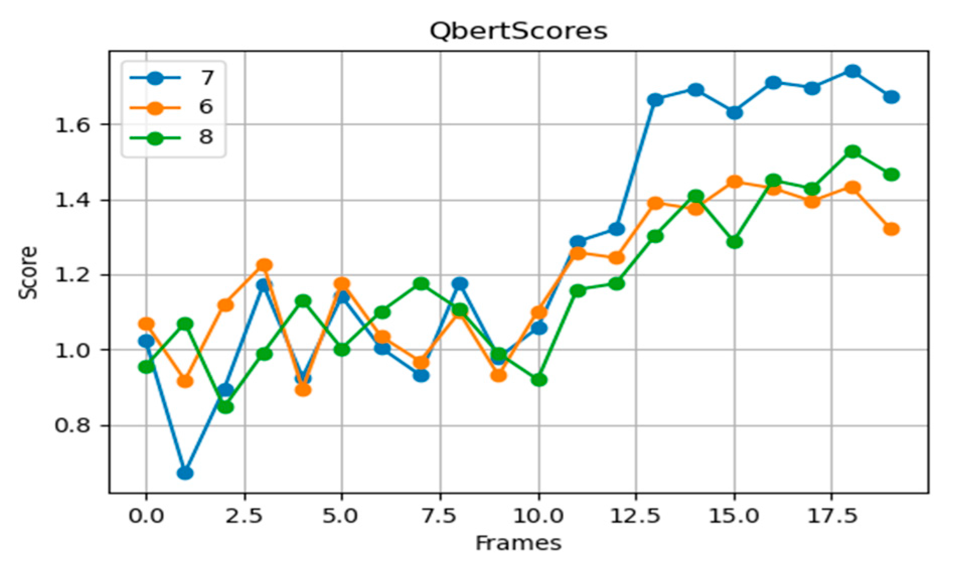
In Q*Bert (Figure 9), the seven-layer network achieves the highest average scores and stability, the six-layer network falls short in strategic adjustments, and the eight-layer network exhibits training instability and strategy overfitting due to excessive depth.

In Enduro (Figure 10), during the early training stages, all depths exhibit similar scores, but differences emerge after 13 million frames. Both the seven-layer and eight-layer networks outperform the six-layer network.

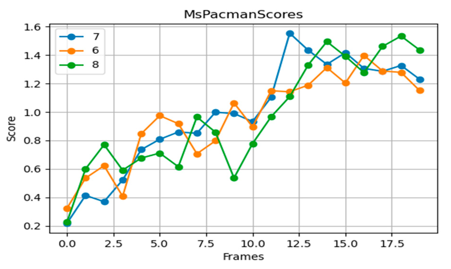
In Ms. Pac-Man (Figure 11), the seven-layer network demonstrates good performance in strategy diversity and score stability. The six-layer network shows slight deficiencies in accurately recognizing complex paths, while the eight-layer network has strategy confusion due to its high complexity.

In Bowling (Figure 12), although network depth varies, scores generally hover around 1, with occasional changes. As a relatively simple game requiring minimal complex strategies or decision processes, even shallower networks can achieve high scores.

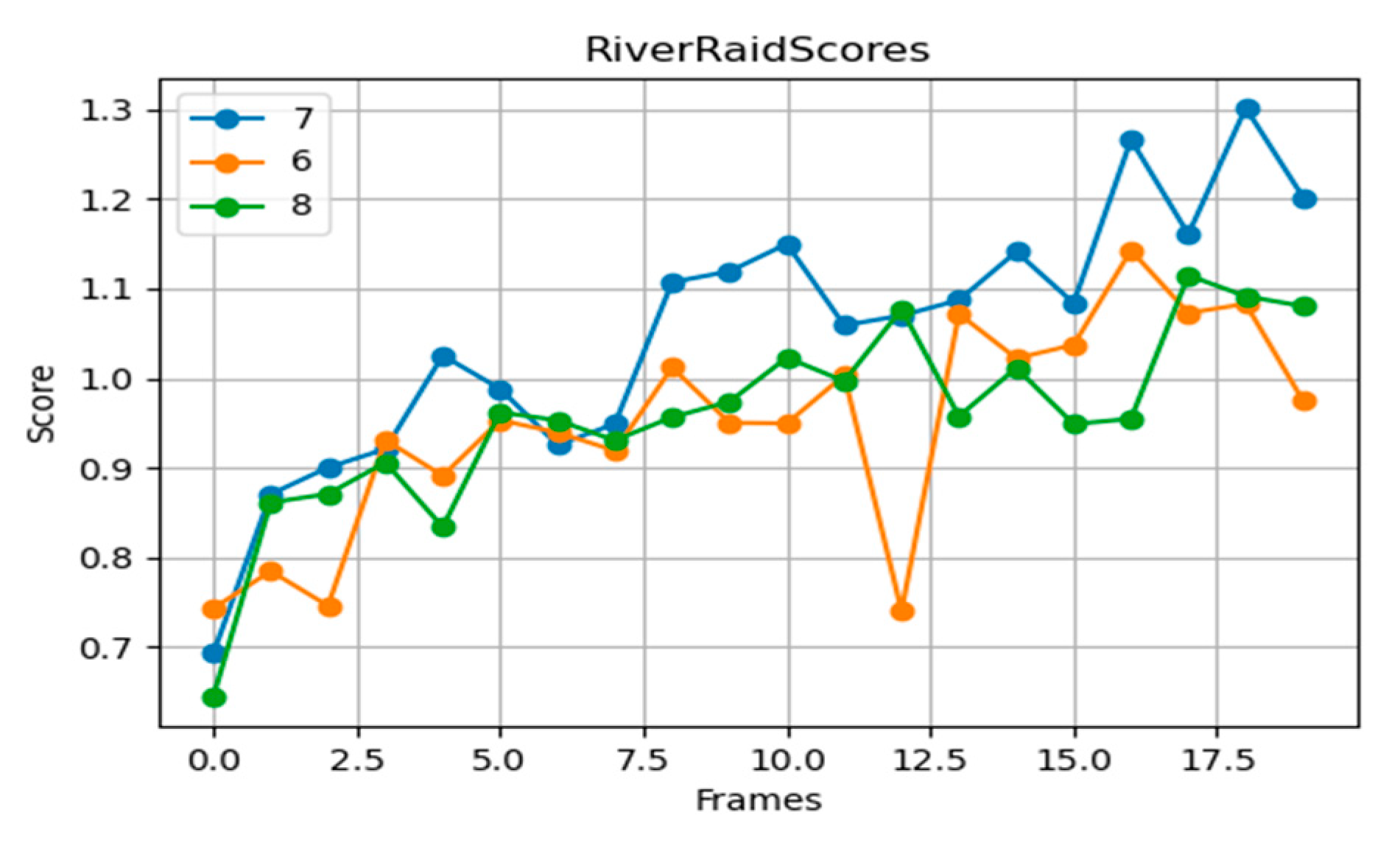
River Raid requires high reaction speed and precise control (Figure 13). The seven-layer network outperforms other depths in both score and stability. Although the eight-layer network can extract complex features, it performs poorly in rapidly changing environments. The six-layer network fails to adequately handle the dynamic environment, showing slower score improvements.

Overall, the seven-layer network performed best in most games, showing good robustness and adaptability. This may be because the seven-layer network has achieved a good balance between feature extraction and policy learning capabilities. It is neither too shallow to capture complex patterns nor too deep to cause overfitting or increased training difficulty. However, in some games (such as Enduro and Bowling), the performance of networks of different depths is not much different. This may be because the environmental complexity of these games is relatively moderate, and the strategy requirements and reaction speed requirements do not significantly enhance the advantages of deep networks. In these scenarios, the choice of network depth does not seem to be the main bottleneck of model performance, so the network design needs to be flexibly adjusted according to specific task requirements.

3.2. Robustness Exploration Against Perturbations

Figure 14 shows the performance of different network depths in the face of external interference (such as image blur and Gaussian noise). The blue line shows the result without image blur, the yellow line shows the result with image blur, and the green line shows the result with Gaussian noise. The experimental results show that the seven-layer network shows the best robustness in the face of external interference such as image blur. This advantage comes from its good balance between depth and feature expression ability, which can effectively extract and utilize environmental features without over-relying on subtle pixel-level information so that it can still maintain a high policy quality when subjected to external interference.

The reason why the seven-layer network shows better robustness may be that it has achieved an appropriate balance in network depth. This balance allows the network to fully extract environmental features while avoiding the overfitting problem that may be caused by too deep networks. Overfitting problems usually occur when the network depth is too large, and the network begins to learn the noise in the data rather than the underlying true pattern, causing the model to perform poorly when facing new and unseen data.

In contrast, although the eight-layer network has better adaptability to blur effects in some cases, this may be because blurring changes the features in the image in an unintuitive way. At certain stages of model training, this feature change may help the model better identify or distinguish certain key features. Overall, the seven-layer network is more robust. This may be because the eight-layer network is too deep, making it more susceptible to overfitting when processing blurred images, or it is difficult to stabilize during network training.

4. Conclusions

Our experimental results in multiple classic reinforcement learning environments, particularly Atari 2600 games, revealed several key findings. First, a seven-layer network architecture demonstrated the best overall performance, balancing feature extraction and policy learning capabilities. This architecture neither suffered from insufficient depth to capture complex patterns nor from overfitting and training difficulties associated with excessive depth. Second, deeper networks exhibited higher risks of overfitting and instability, especially in rapidly changing or complex game environments. In contrast, shallower networks struggled to handle complex dynamics and strategic adjustments required by certain games. We also conducted robustness tests by introducing external perturbations such as image blurring. The results indicated that the seven-layer network maintained the best performance under these conditions, suggesting its superior robustness. This can be attributed to the appropriate balance in network depth, allowing effective feature extraction without overfitting to noise.

Furthermore, our analysis of network architecture design highlighted the importance of adaptive configurations based on task complexity. The proposed adaptive deep Q-Dagger network architecture, which dynamically adjusts depth according to factors like state space size, reward sparsity, and action space size, proved effective in enhancing model flexibility and performance across diverse tasks. In summary, this study provides comprehensive guidance for designing and optimizing regenerative reinforcement learning models. By thoroughly exploring the relationship between network depth and model robustness, our findings establish a theoretical foundation for developing more efficient and stable reinforcement learning models. Although the experimental results show that the proposed architecture exhibits high robustness and excellent performance in multiple Atari 2600 games, the verification of this study mainly focuses on a small number of classic environments and does not fully explore other influencing factors such as network width, activation function, and regularization strategy. Therefore, the generalization ability of this method still needs to be further verified in larger-scale, more complex, or diverse task environments.