A Novel Earth-System Spatial Grid Model: ISEA4H-ESSG for Multi-Layer Geoscience Data Integration and Analysis

Abstract

This paper presents a novel Earth-System Stratified Grid (ISEA4H-ESSG) model, designed to address the challenges in multi-layer geoscience data management and analysis. In the realm of geosciences, which encompasses the solid earth, atmosphere, hydrosphere, and biosphere, as well as planetary and space sciences, the effective integration of diverse data sources is crucial. Traditional grids have limitations in three-dimensional spatial modeling, cross-layer data fusion, and dynamic multi-scale analysis. The ISEA4H-ESSG model overcomes these drawbacks by integrating the Icosahedral Snyder Equal-Area Aperture 4 Hexagon Discrete Global Grid System (ISEA4H DGGS) with a degenerative subdivision mechanism. It adheres to six core principles, including stratified spherical coverage, geographic consistency, multi-scale dynamic adaptability, global seamless partitioning, encoding uniqueness and efficiency, and multi-source data compatibility. Through the independent subdivision of spherical and radial layers, this model balances resolution differences and resolves polar-grid distortion and cross-layer data heterogeneity issues. The introduction of a four-dimensional spatiotemporal encoding framework enhances the storage and parallel computing capabilities of massive datasets. Case studies on ionosphere three-dimensional modeling and global atmospheric temperature field formatting demonstrate the high precision and adaptability of the ISEA4H-ESSG model. This research provides a unified spatial data infrastructure for geosciences, facilitating in-depth studies on natural hazards, climate change, and planetary evolution, and offering new perspectives for international partnerships and future Earth-related research.

1. Introduction

1.1. Background and Motivation

With the increasing scientific exploration and production activities on a global scale, human focus has expanded beyond the Earth’s surface to include subsurface domains, underwater environments, and near-Earth space. Attention to global issues now spans phenomena such as internal plate tectonics, crustal movements, atmospheric dynamics, and ionospheric variations in near-Earth space [1]. Global challenges—such as climate change, pollution, and natural disasters—stem from interactions across Earth’s spheres. Addressing these challenges cannot rely solely on a single discipline or the study of a single Earth layer; it necessitates in-depth research into multi-layer interactions and a holistic understanding of the Earth system [2,3]. Beyond the efficient organization of surface spatial data, there is an urgent demand for the integrated management of atmospheric and near-Earth spatial information across Earth’s spheres.

1.2. Current Status of Multi-Layer Observational Data in the Earth System

Atmospheric space is key for spacecraft monitoring, where atmospheric processes and astronomical phenomena significantly impact human societal development and daily life. Key physical characteristics of the atmospheric environment include temperature, humidity, wind speed, and air pressure [4]. Ground-based observatories, weather balloons, lidar systems, and meteorological satellites are employed to detect and record parameters such as atmospheric wind fields, temperature fields, and humidity. Near-Earth space, spanning approximately 100 km to 35,786 km above the Earth’s surface, is the orbital region for spacecraft. Environmental factors in this domain encompass the ionosphere, magnetic-field parameters, and space radiation. Terrestrial, oceanic, airborne, and satellite-based monitoring networks currently form the primary observational infrastructure for near-Earth space environments [4,5]. Observing and simulating atmospheric and near-Earth space dynamics are vital scientific endeavors, commonly relying on supercomputers, sensor networks, and operational modeling systems to analyze and predict environmental changes. However, the complex three-dimensional structures of atmospheric phenomena, combined with large spatial and temporal data scales, pose significant challenges for precise vertical stratification modeling and computation. A three-dimensional spatial grid covering the atmospheric sphere is essential for organizing atmospheric and near-Earth data and enabling synergistic analysis with surface-layer data [6].

Since the beginning of the 21st century, satellite remote sensing has evolved into an integrated space–air–ground observation system, becoming a pivotal tool for surveying, monitoring, analyzing, and forecasting resources, environments, disasters, regions, and urban areas. Advances in Earth observation technologies and computational capabilities have enabled the acquisition of multi-source, multi-dimensional, and massive multi-layer geospatial datasets through remote sensing and numerical modeling. These datasets include surface data (e.g., natural disaster records, land-use patterns), atmospheric layer data (e.g., wind fields, temperature profiles) [6,7], and ionospheric data (e.g., electron density, total electron content), providing a foundational resource for multi-layer Earth-system research [5]. Rapid advancements in space exploration and data acquisition technologies have expanded the scope of spatial phenomena monitoring, achieving increasingly finer granularity in information collection.

These datasets—encompassing traditional digital maps, remote sensing imagery, and specialized data from meteorology, disaster studies, hydrology, and geophysics—require systematic organization, management, modeling, analysis, and visualization to transform raw data into interpretable spatial information. Such processed information is crucial for analyzing spatial patterns and uncovering underlying principles [8]. However, contemporary human activities exhibit globally distributed, multi-layered, multi-scale, and cross-disciplinary characteristics, necessitating a unified global spatial framework to integrate massive, heterogeneous data across Earth’s spheres. Challenges arise from significant disparities in data storage formats, syntactic structures, processing tools, and management protocols across disciplines, creating disciplinary barriers and technical obstacles that hinder interdisciplinary, multi-scale, and cross-layer Earth-system research [9]. Furthermore, the reliance on latitude-longitude grid systems for multi-layer observational data exacerbates structural inequivalence in grid resolution across low-, mid-, and high-latitude regions (particularly at the poles), leading to regionalized model parameters and impeding global-scale or large-scale interaction studies. This limitation becomes even more pronounced in multi-layer research contexts.

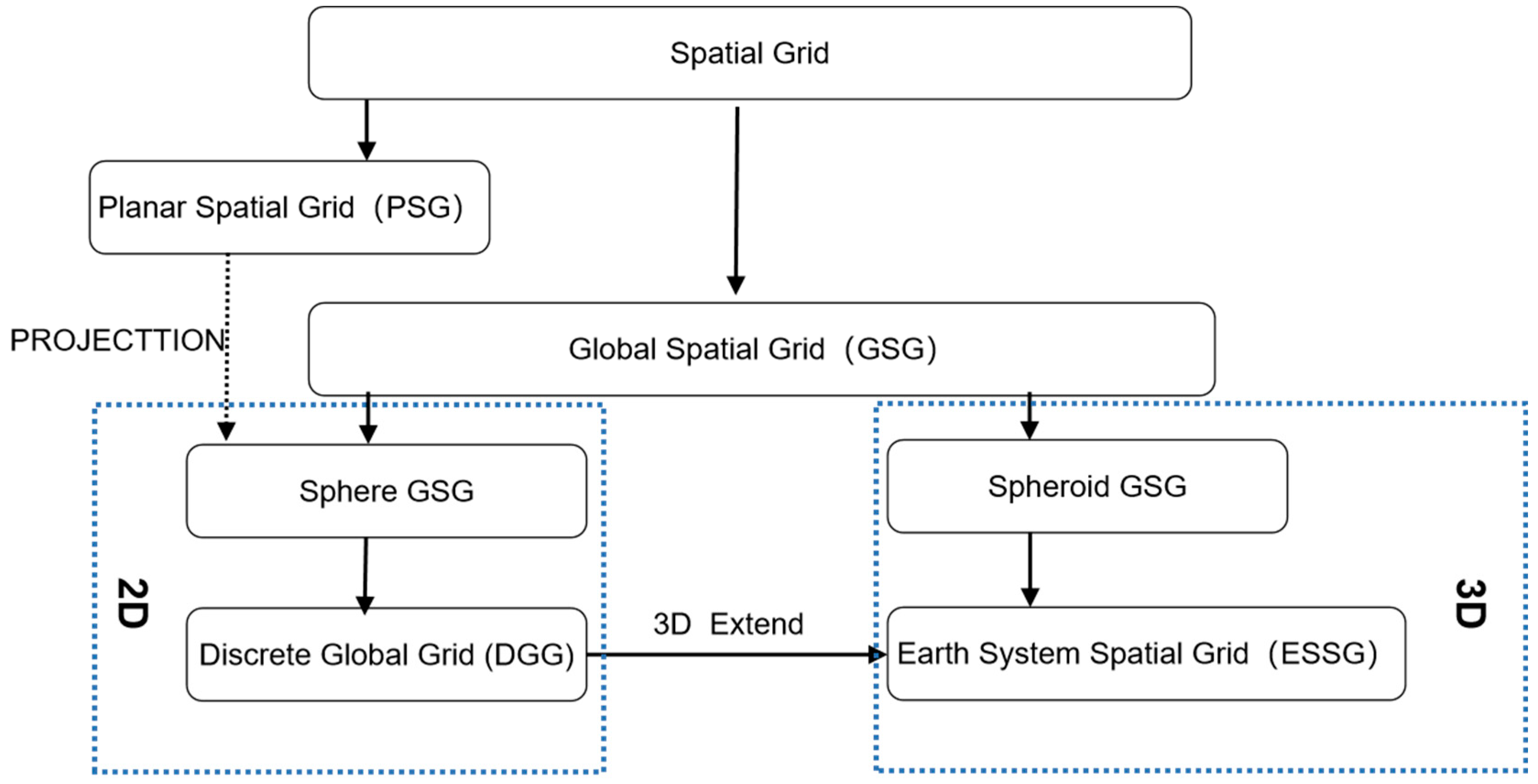
1.3. Current Research Status of Earth Spatial Grid

Spatial grids are categorized into Planar Spatial Grids (PSGs) and Global Spatial Grids (GSGs). PSGs partition planar spaces based on Euclidean geometry, with common types including quadtree grids, finite-element grids, square grids, and Triangulated Irregular Networks (TINs). GSGs, on the other hand, divide global spaces based on spherical or spheroidal manifolds, further classified into spherical GSGs (2D manifolds) and spheroidal GSGs (3D manifolds). Discrete Global Grid Systems (DGGS) uniformly discretize Earth’s space into seamless, non-overlapping multi-resolution hierarchical grids. These systems inherently support the unified modeling of multi-layer Earth observation data, enabling multi-scale, multi-resolution, and multi-level data integration while offering flexibility in representing vertical elevation information in near-Earth space [10,11,12]. Additionally, the homogeneous structure of DGGS enhances the generalization and adaptability of multi-layer analytical models at global scales, and their discrete data organization and encoding-based operations align well with cloud computing and big data environments [13]. Wu Lixin et al. proposed that universal sphere GSG oriented to the Earth system can be called the Earth-System Spatial Grid (ESSG) [6]. The classification system of global spatial grid is shown in Figure 1.

Spherical spatial grids (or Discrete Global Grids, DGGs) typically generate discrete units through the recursive subdivision of (ellipsoidal) spheres to support multi-scale data organization and modeling [14]. Existing DGGs can be divided into two categories:

A.

Latitude–Longitude Grids

These grids partition the sphere using latitude and longitude lines, divided into equidistant and variable-interval types. Equidistant grids (e.g., GTOPO30 [15], ETOPO5 [16]) are structurally simple but suffer from high-latitude grid distortion (quadrilaterals → rhombuses → triangles) [17], leading to data redundancy and reduced accuracy. Variable-interval grids (e.g., GTED, Spherical Degenerated Quadtree [18]) mitigate distortion by adjusting latitude band intervals but increase model complexity.

B.

Regular Polyhedron-Based Grids

These grids use regular polyhedrons (tetrahedrons, hexahedrons, octahedrons, etc.) as base surfaces, constructing approximately uniform grids through subdivision and projection. Regular polyhedron-based grids, summarized in

Table 1. Regular polyhedron-based grids.

Grid Type	Structural Features	Representative Models	Advantages and Limitations	Typical Applications
Triangular Grids	Based on octahedrons/icosahedrons; hierarchical but geometrically complex	QTM (Quaternary Triangular Mesh) [19] SQT (Sphere Quad Tree) [20]	Pros: Hierarchical continuity Cons: Complex neighborhood algorithms, irreducible geometric distortion	Global terrain modeling Spatial indexing
Quadrilateral Grids	Merged triangular units; simplified adjacency relations	Octahedral rhombus subdivision Quadtree-extended models	Pros: Simplified neighborhood operations Cons: Limited flexibility, minor high-latitude distortion	Data visualization Hierarchical analysis
Hexagonal Grids	High adjacency symmetry; optimal coverage efficiency	H3 (seven-aperture) rHEALPix (refined Hierarchical Equal-Area iso-Latitude Pixelization) [21] OHQS (Optimized Hexagonal Quadtree Structure) [22]	Pros: Dynamic modeling performance Cons: High encoding complexity, projection approximation required	Global environmental sampling Multi-resolution platforms

Note: QTM: Quaternary Triangular Mesh; SQT: Sphere Quad Tree; H3: Uber’s open-source hexagonal grid system; rHEALPix: refined Hierarchical Equal-Area Pixelization; OHQS: Optimized Hexagonal Quadtree Structure.

, include triangular, quadrilateral, and hexagonal types, each with distinct advantages and limitations.

Because of their different division and coding structure, these grids have different characteristics in application. For example. H3, developed by Uber (2018) [23], leverages a seven-aperture hexagonal structure, offering high computational efficiency with encoding requiring approximately 32 bits per cell and fast retrieval times due to its hierarchical indexing. However, its focus on surface-level applications limits its vertical stratification capabilities for 3D modeling. In contrast, rHEALPix (Gibb 2016 [21]) provides equal-area pixelization with adjustable resolution, excelling in global environmental sampling, but its complex projection adjustments increase the computational overhead by 15–20% compared to simpler grids like latitude–longitude systems (Purss et al. 2019 [17]). Real-world applications, such as H3’s use in ride-sharing optimization, prioritize speed over multi-layer integration, while rHEALPix supports climate modeling but struggles with dynamic vertical data fusion.” These comparisons are grounded in published documentation (Uber 2018 [23]; Gibb 2016 [21]) and our analysis of their performance metrics. However, existing spherical-grid models primarily focus on Earth’s surface and lack rigorous grid-based modeling for the vertical 3D space (near-Earth space) along Earth’s diameter, making it challenging to scientifically describe 3D spatial entities, processes, and information.

Spheroidal spatial grid research, often framed within Earth-system science and global-scale challenges, targets medium- to ultra-large-scale phenomena such as tectonic plate movements, regional geological activities, atmospheric and oceanic circulation, ionospheric dynamics, geomagnetic fields, and near-Earth environmental interactions. Commonly used spheroidal grid systems include:

• Latitude–longitude spheroidal grids: Extend 2D grids radially but suffer from polar distortion [24].
• Cubed-sphere grids: Use cubic projections for uniform coverage, suited for atmospheric modeling [25].
• Yin–Yang Grid: Designed for mantle convection with overlapping domains [26].
• Adaptive Mesh Refinement (AMR): Dynamically adjusts resolution for localized phenomena [27].
• Sphere Degenerated Octree Grid (SDOG): Employs octree subdivision for 3D Earth modeling but lacks flexible layering [28].

This numbered format enhances clarity and allows readers to quickly grasp the diversity of spheroidal grids.

These grids exhibit domain-specific innovations tailored to distinct Earth-system applications.

The evolution of Earth spatial grids has progressed from local planar grids to 3D grids, and from spherical grids to spheroidal grids. While spherical grids abstract Earth’s space as a surface, suitable for representing surface-level phenomena, they fail to rigorously model 3D objects [29]. Spheroidal grids treat Earth as a homogeneous sphere with radial hierarchies, but these hierarchies cannot be flexibly adjusted—they rely on radial subdivision to approximate predefined spherical layers, inadequately capturing true layered structure. Spheroidal grids (e.g., SDOG) approximate layers radially yet struggle with flexible stratification [28]. For instance, SDOG approximates atmospheric layers but cannot flexibly adjust to the ionosphere’s variable thickness [28]. ISEA4H-ESSG bridges these gaps with adaptive 3D layering.

Spatial phenomena and processes interact across scales, necessitating a unified multi-scale 3D grid framework for coupled modeling. Constructing a layered and adapted 3D grid with figures requires adaptive modifications in grid design, subdivision encoding, and data models to align with Earth’s layered structure. Such a framework must not only describe activities within individual layers but also unify cross-layer spatial representations, ultimately establishing an integrated spatial framework encompassing terrestrial, atmospheric, and celestial domains.

2. Materials and Methods

This section outlines a series of methods for constructing the Earth-System Stratified Grid (ESSG). First, based on the principles and requirements of Discrete Global Grid (DGG) construction, we propose criteria for building a three-dimensional Earth-System Spatiotemporal Grid (The Earth-System Spatial Grid (ESSG), also termed Spatiotemporal Grid due to its temporal encoding, is a unified 3D framework). Second, we elaborate on the subdivision and encoding methods of this grid system across spatial dimensions (stratified layers and radial layers) and temporal dimensions.

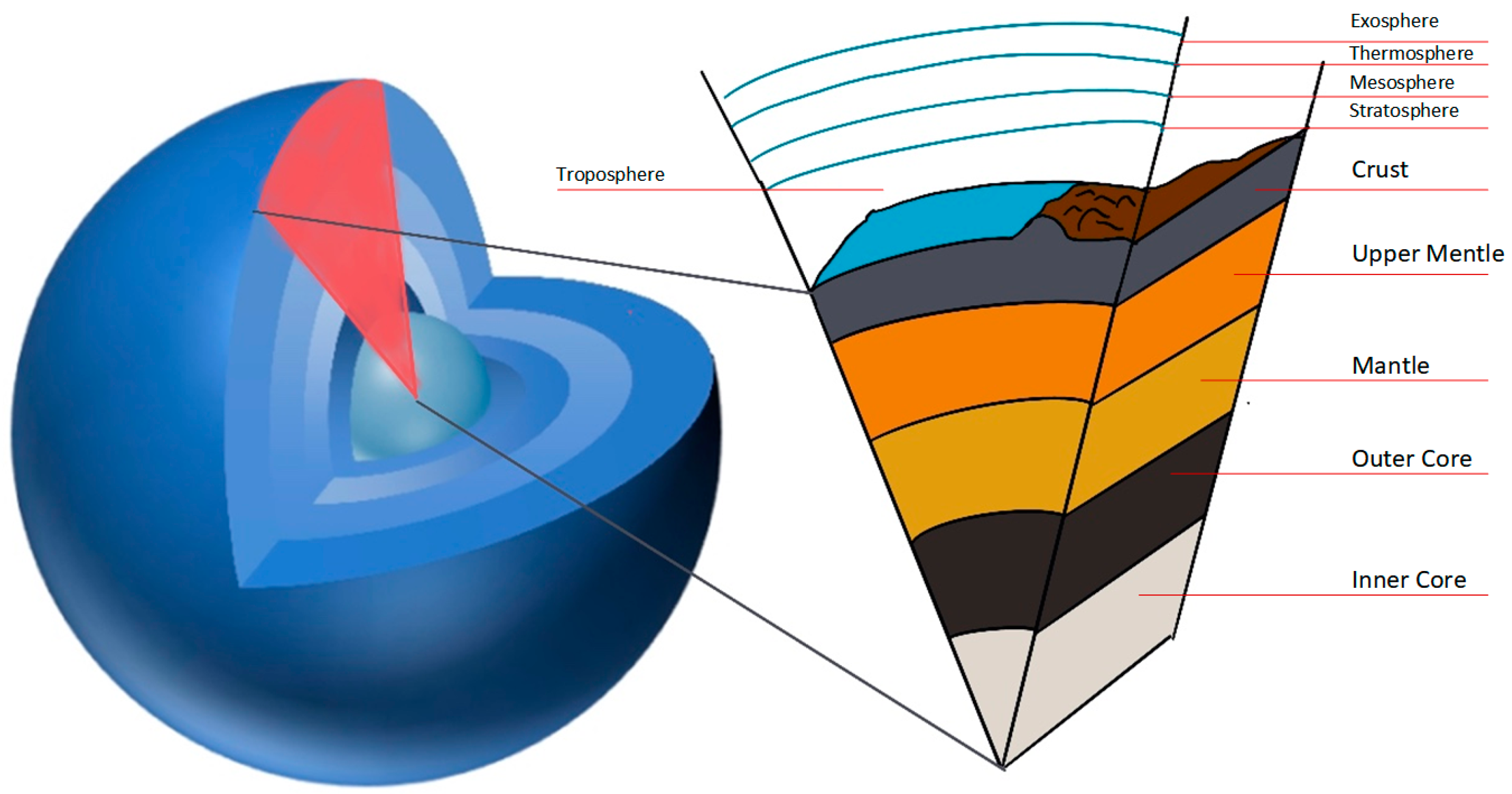
2.1. Requirements for the Earth-System Spatial Grid

2.1.1. Definition of the Earth-System Spatiotemporal Grid

The Earth-System Spatial Grid is a unified global grid constructed for the entire three-dimensional Earth space. It mathematically abstracts Earth’s volumetric space into an Earth-system space, studies hierarchical subdivision and encoding of this space, and discretizes it into a series of grid cells following specific rules. Each cell possesses a unique identifier, enabling the description and modeling of entities, processes, spatial relationships, and interactions. This framework supports the integrated organization and storage management of data.

2.1.2. Principles and Requirements for the Earth-System Spatial Grid

In 1994, Goodchild was the first to propose the basic criteria for the division of the Discrete Global Grid (DGG), which include shape consistency. That is, the shapes of the grid cells should be kept as consistent as possible to reduce the errors generated during analysis and processing due to shape differences. It also includes recursive subdivisibility, which enables the grid to be recursively subdivided according to specific rules, meeting the requirements of data processing with different precisions and facilitating the effective description of the geographical space at different scales. Geographical correspondence is another criterion, ensuring that there is a clear correspondence between the grid and geographical coordinates, making it convenient for the conversion of geographical data between the traditional coordinate system and the grid system [30].

In 1999, Kimerling improved on Goodchild’s research findings and established the Kimerling standard [31]. This standard covers several core elements: multi-level nature; area approximation; shape approximation; universality; recognizability; and simplicity of conversion with latitude and longitude coordinates. The Kimerling standard is also regarded as the core of the evaluation criteria for DGG division.

However, this standard has limitations when facing the complex multi-layered structure of the Earth system, massive dynamic data, and special research requirements. The Kimerling standard excels for 2D grids but lacks criteria for 3D vertical stratification, dynamic multi-layer data fusion, and real-time adaptability required by Earth-system science [31]. In order to describe the Earth system more comprehensively and accurately, meet the unique needs of cross-layer, multi-scale, dynamic change research, and multi-source data-fusion analysis, and promote the in-depth development of Earth-system science research, this paper, based on the above ideas, proposes the six criteria of ESSG (Earth-System Space Grid) for the Earth-system space.

(1)

Stratified Spherical Coverage Criterion

This criterion mandates seamless, gap-free grid coverage across all volumetric layers, extending from Earth’s surface to the lithosphere and upward to the ionosphere.

Closely related to Kimerling’s “Global Coverage” principle, this criterion expands its scope from 2D surface coverage to 3D volumetric space. For example, in seismic studies, grids must penetrate the lithosphere to precisely map seismic wave propagation and energy release, aiding earthquake prediction. In atmospheric research, grids must vertically span from the troposphere to the stratosphere to track ozone, water vapor, and greenhouse gas dynamics, supporting climate studies and pollution control.

(2)

Geographic Consistency Criterion

Geographic consistency refers to the alignment of Earth-system phenomena with latitude–longitude distributions, reflecting natural geographic patterns (e.g., topography, climate zones, ocean currents). Earth’s rotation and revolution further drive latitudinal and seasonal variations in solar radiation, influencing climate, hydrology, biology, and soil distribution. Human activities and existing geographic datasets (largely based on latitude–longitude systems) also reinforce this spatial cognition.

This criterion requires ESSG to align with Earth’s natural features, human cognitive habits, and existing data frameworks. Grid boundaries should align with meridians, parallels, or key geographic boundaries to intuitively reflect phenomena locations. Compatibility with latitude–longitude systems minimizes data conversion costs, enhances processing efficiency, and improves usability. ESSG must enable bidirectional conversion between grid cells and geographic coordinates.

(3)

Multi-Scale Dynamic Adaptability Criterion

Earth-system phenomena exhibit multi-scale spatiotemporal characteristics, from long-term climate cycles (e.g., glacial–interglacial shifts) to short-term meteorological events (e.g., thunderstorms), and from continental drift to localized seismic activity. This criterion demands grids that capture macro-scale trends (e.g., ocean circulation, ecosystem patterns) and micro-scale details (e.g., urban heat islands, soil erosion).

Building on Kimerling’s “Hierarchy” and “Scalability” principles, this criterion emphasizes real-time or near-real-time tracking of dynamic changes. For instance, in wildfire monitoring, low-resolution grids rapidly identify fire-prone areas, while dynamic refinement to high-resolution grids tracks fire spread and ecological impacts, enhancing disaster response.

ESSG must support asynchronous multi-resolution grids—infinitely subdivisible and adaptable across dimensions—to address diverse application needs.

(4)

Global Seamless Partitioning Criterion

Earth’s volumetric space spans from its core to outer space. This criterion requires grids to fully and seamlessly cover this domain, accounting for Earth’s non-spherical geometry, surface topography (mountains, oceans, canyons), and heterogeneous layer thicknesses. Grids must naturally transition between terrestrial, marine, and atmospheric regions, including extreme terrains like ocean trenches and mid-ocean ridges. Extending Kimerling’s “Global Coverage” to 3D, this principle ensures comprehensive data foundations for multi-layer research.

(5)

Encoding Uniqueness and Efficiency Criterion

The uniqueness and high efficiency of coding require each grid unit to have a unique coding and support efficient coding and decoding operations. The spatial data of the Earth system are massive and complex, and the traditional latitude and longitude coding method is inefficient at high resolution. The criterion of coding uniqueness and high efficiency requires the grid system to adopt a compact and unique coding scheme, to ensure that each grid unit has a unique logo on a global scale, and to support efficient coding, decoding, and spatial indexing operations. This high efficiency can not only improve the efficiency of data storage and retrieval, but also support the real-time processing and analysis of large-scale spatial data, providing more efficient computing support for multi-layer research.

(6)

Data Fusion and Multi-Source Compatibility Criterion

ESSG must integrate multi-source data (remote sensing, ground observations, simulations) with varying formats, resolutions, and semantics. A unified fusion framework ensures seamless interoperability, improving data utilization efficiency and enabling cross-layer analysis.

The Earth-system space grid represents a new development direction for geographical space grids, evolving from planar grids to three-dimensional grids, and from spherical grids to spherical body grids, and extending to the Earth’s layered space.

Looking back on the construction concepts of spherical grids and spherical-body grids, spherical space grids abstract the Earth’s space into a spherical space, which is suitable for expressing various spatial objects on the Earth’s surface. However, it is difficult to scientifically and rigorously describe the three-dimensional objects within the Earth’s space. On the other hand, spherical-body space grids abstract the Earth’s space into a spherical body space. In essence, they regard the Earth’s space as a sphere with a uniform interior. Although there is also a radial hierarchical structure, this hierarchical structure cannot be adjusted as needed. It can only approach the given layer plane as closely as possible through radial subdivision, and it does not fully reflect the characteristics of the layered structure. Therefore, simply abstracting the Earth’s layered space into a spherical body is insufficient for constructing a layered space grid. It is necessary to abstract the characteristics of the Earth system’s layered structure into a layered space, which serves as the mathematical model basis for constructing the layered space grid.

2.2. ISEA4H Subdivision Model of the Temporal and Spatial Grid of the Earth System’s Layers

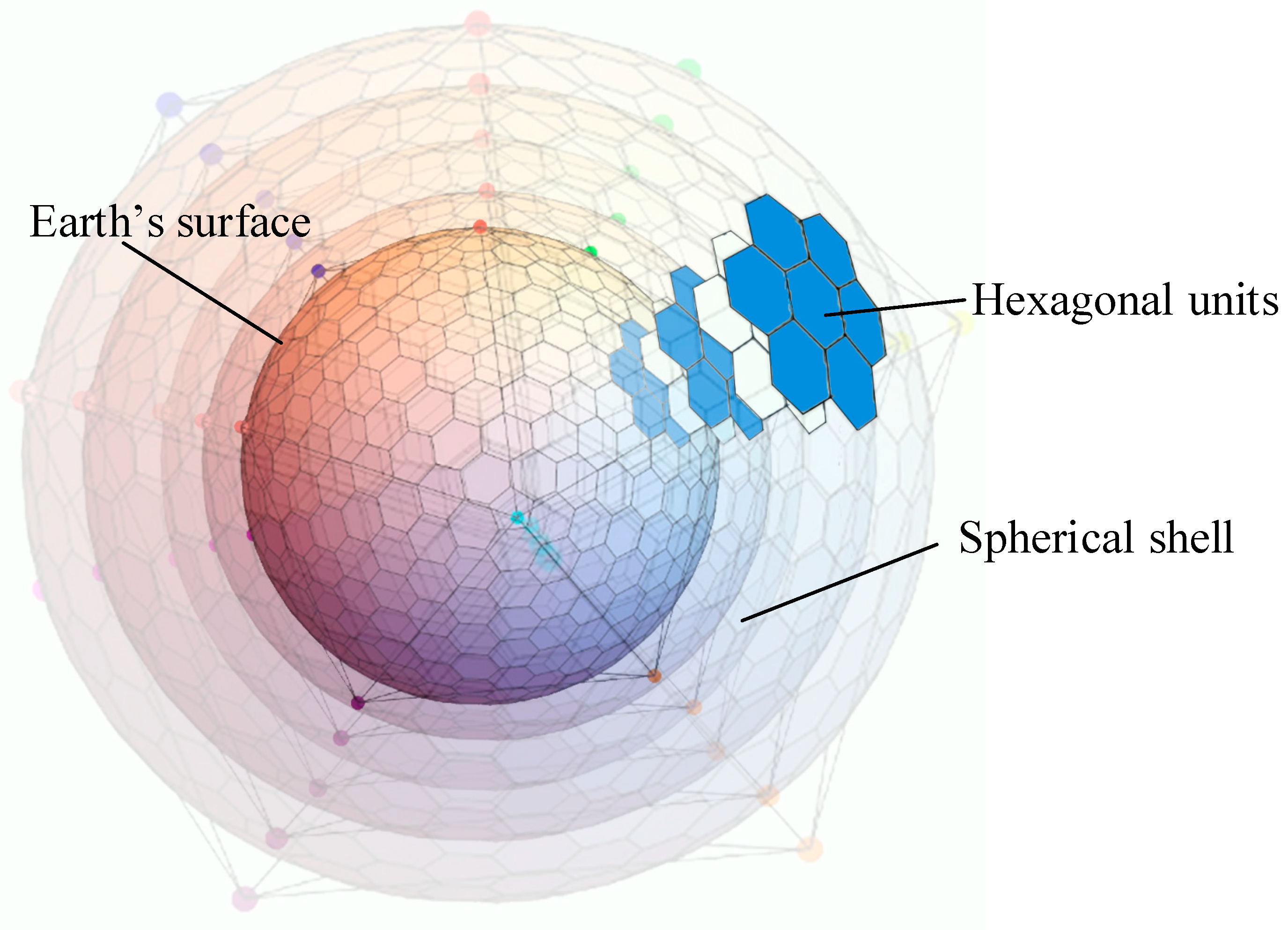
2.2.1. Basic Concept

In order to clearly describe the Earth’s layers in a gridded and hierarchical manner, it is necessary to first clarify the scope and concept of the Earth’s layers. Intuitively, as shown in Figure 2, the layered structure of the Earth system is manifested as a series of spherical shells divided by concentric spherical surfaces with the Earth’s center as the center of the sphere. These spherical shells are located between the inner and outer spherical surfaces and have a certain thickness. The innermost layer is a sphere; that is, the radius of the inner spherical surface is 0, and the center of the spatial region of the Earth system’s layers is the Earth’s center.

For the position of any point in the spatial region of the Earth’s layers, it can be represented based on the coordinates of the geocentric polar coordinate system $(\mathrm{r},\mathsf{\lambda },\mathsf{\phi })$, where the distance from this point to the Earth’s center is the radius $\mathrm{r}$.

For the entire Earth system’s layered space, it can be divided into layer bodies and layer surfaces. Among them, according to the Earth’s layered structure, some layer surfaces are called reference layer surfaces.

Layer Body: A spherical shell defined by radius r between inner radius R and outer radius R′ (r[R, R′]). Layer Surface: A spherical surface Sr at radius r from Earth’s center.

Layer Surface: The layer surface is a spherical surface with the Earth’s center as the center of the sphere, which is used to divide different layers and can be expressed as Sr.

Reference Layer Surface: The layer surface that divides the inner and outer layers is set according to the layer surface of the Earth’s surface on which the global discrete grid is established. According to the layered structure of the Earth system, taking the reference layer surface as the boundary, it can be divided into the inner layers of the Earth, the Earth’s surface, the outer layers of the Earth, etc. Among them, the inner layers include the Earth’s core, mantle, crust, etc.; the Earth’s surface includes the lithosphere, hydrosphere, biosphere, etc., and the outer space includes the atmosphere, near-Earth space, etc.

The result of subdividing the layered space of the Earth system is a three-dimensional space grid unit with variable layers at each subdivision level. At the same time, the layer surface is also divided into corresponding grid units. The layer-surface grid is a spherical grid formed on each layer surface during the process of subdividing the three-dimensional space of the Earth system. The subdivision units on the layer surface are called layer cells.

2.2.2. Design Concept of the ISEA4H-ESSG Subdivision Model of the Temporal and Spatial Grid of the Earth System’s Layers

The ISEA4H-ESSG temporal and spatial grid of the Earth system’s layers needs to reflect, as much as possible, the natural spherical layered structure of the Earth system, as well as the trends in the vertical (radial) and horizontal (spherical) directions, that is, the layered structure. Therefore, the ISEA4H-ESSG should take the geocentric coordinate system as the spatial reference, use the Earth’s spherical surface as the starting surface, and demarcate the reference layer surface according to the distribution characteristics of the layers of spatial activities and spatial information. The initial layer body is constructed by using the initial layer cells of the adjacent reference layer surfaces. The subdivision is carried out on the reference layer surface based on the subdivision structure of the four-aperture global discrete grid of the regular icosahedron, and the subdivided grid units are extended to the Earth’s space, discretizing the entire Earth’s space into three-dimensional grid units with equal areas at each subdivision level. The layer bodies of adjacent subdivision levels have a spatial subordination relationship. Each layer body has a unique global code and corresponds to a three-dimensional spatial region in the Earth’s space, which is used to organize various information in the region of the grid unit. The layered spatial grid seamlessly covers the entire Earth’s space and becomes a unified framework for various spatial information in each layer of the Earth system. Figure 3 is a conceptual diagram of the ISEA4H-ESSG layers, showing the starting surface (Earth’s surface), initial layer body (spherical shell), and layer cells (hexagonal units).

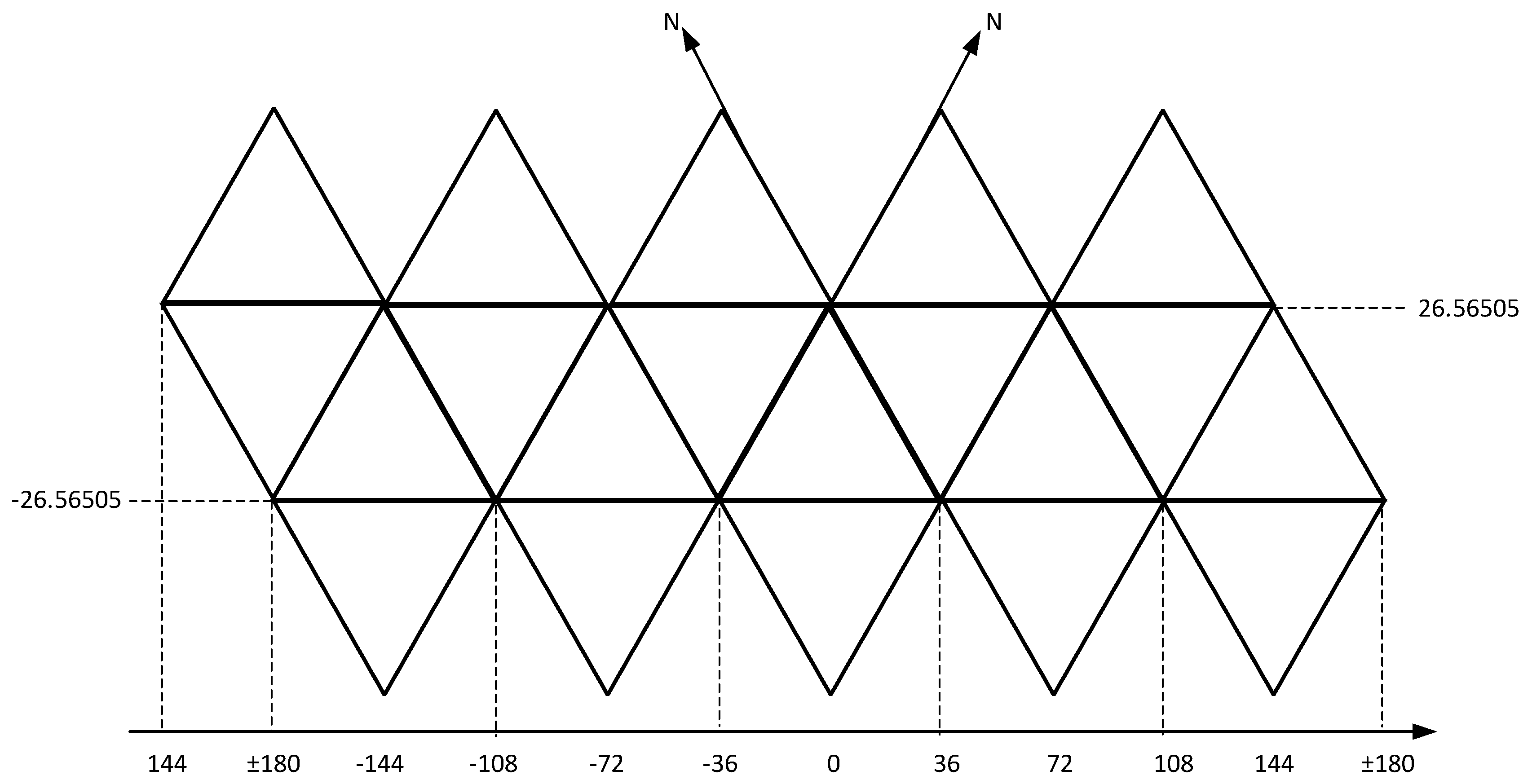
2.2.3. Subdivision Mechanism of the ISEA4H-ESSG Temporal and Spatial Grid of the Earth System’s Layers

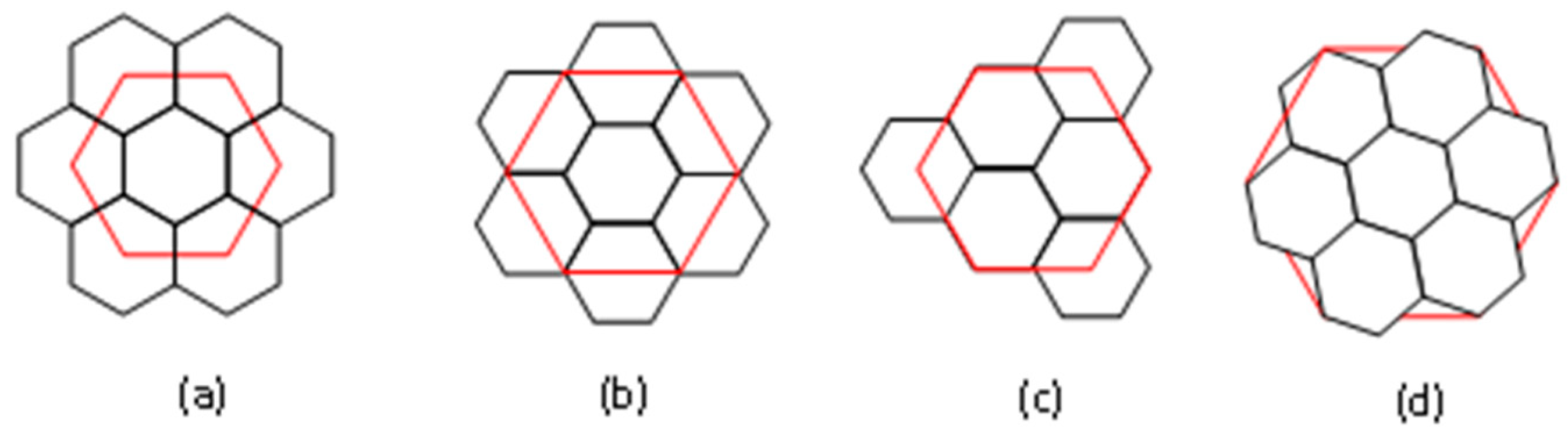
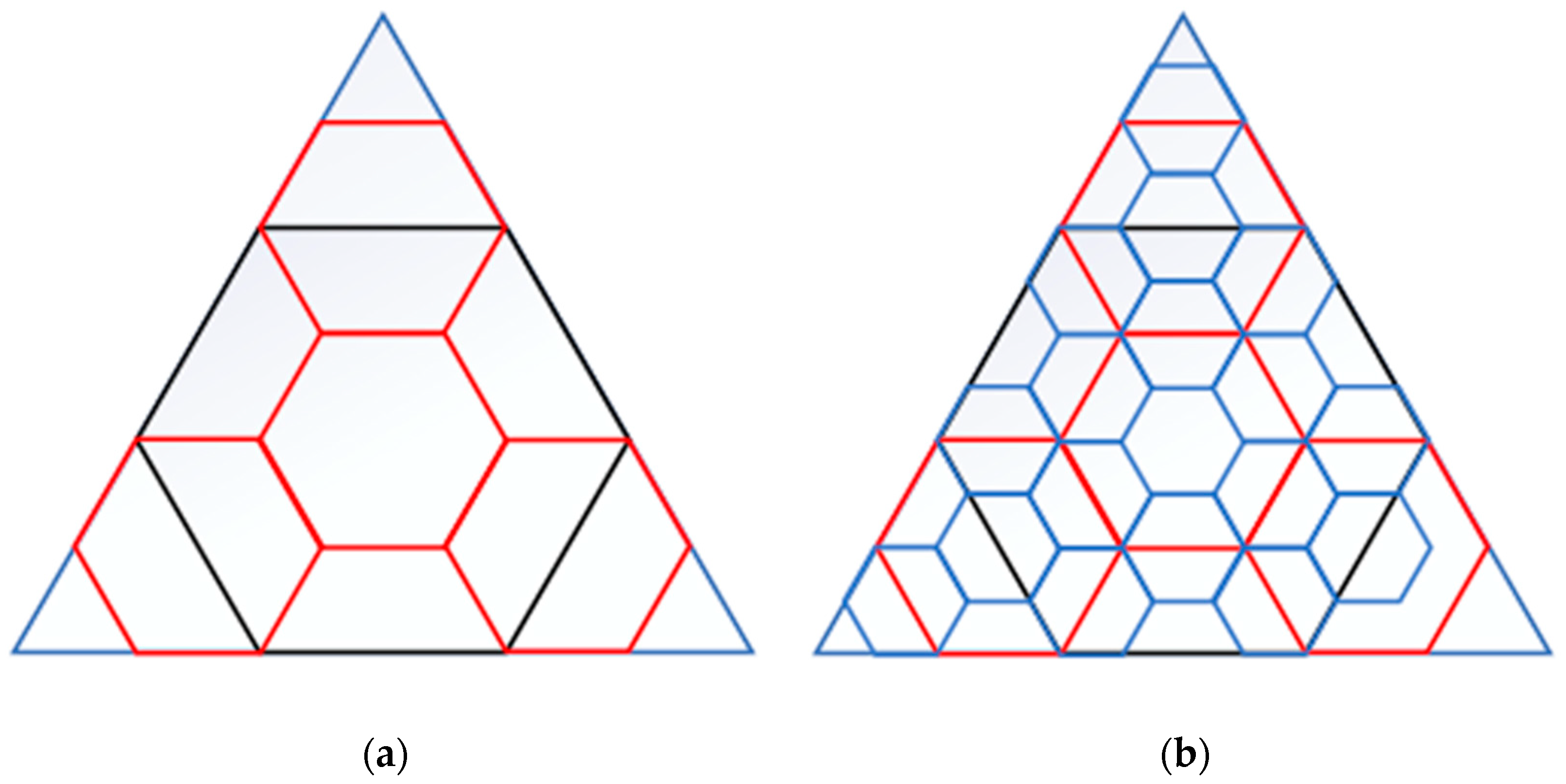
Unlike local planar or 3D Euclidean grids, the layered spatial grid extends spherical subdivision to near-Earth space, necessitating a distinct mechanism. The spherical-grid subdivision mechanism recursively divides a sphere (e.g., via ISEA4H’s hexagonal tiling) into equal-area units [32], which we extend radially for 3D layering. The subdivision mechanism of a spatial grid is usually determined by the characteristics of the subdivided object and the subdivision requirements. For the planar and three-dimensional grid subdivision of the local Earth area, it is generally established in the coordinate system of Euclidean space indices, and the space is subdivided in each spatial dimension. The spatial subdivision mechanism of the layered spatial grid will be extended in the height range from the spherical surface to the near-Earth space based on the spherical-grid subdivision mechanism.

(1)

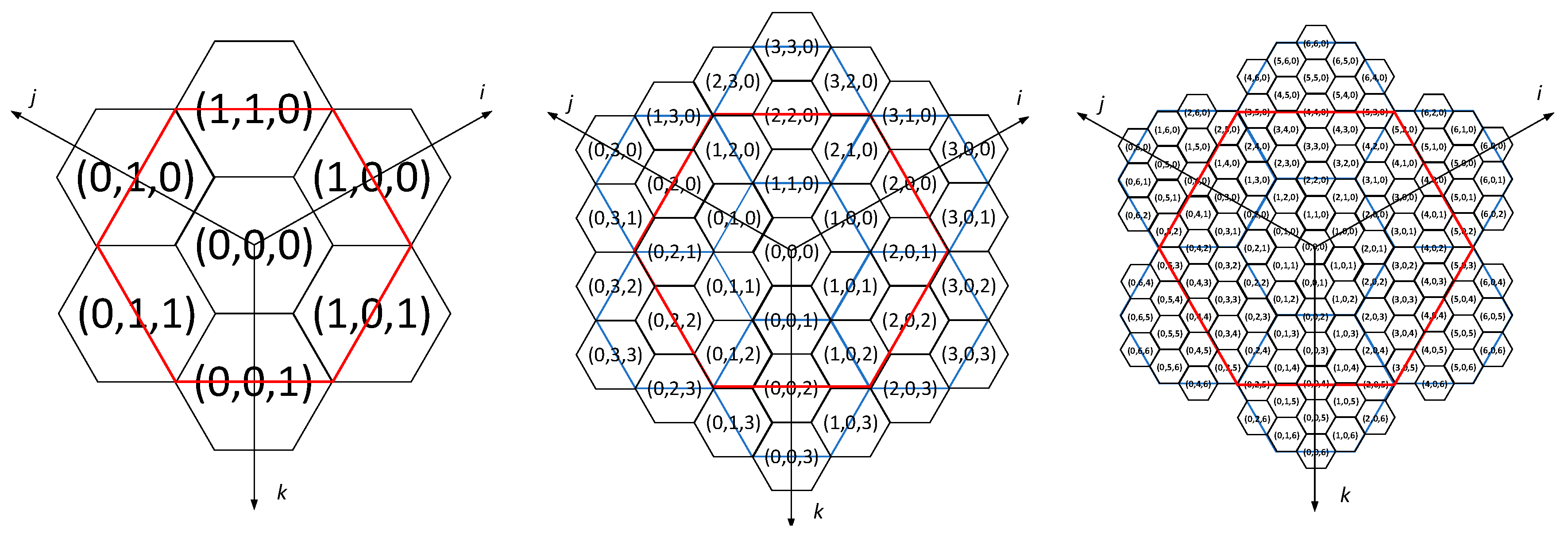
Subdivision of the Four-Aperture Hexagonal Global Discrete Grid

The basic model to be adopted is the Icosahedral Snyder Equal-Area Projection Aperture 4 Hexagon Discrete Global Grid System (ISEA4H DGGS) [32]. For the spherical spatial grid on the Earth’s surface, the IEEA4H DGGS is used to construct a multi-level grid for spherical subdivision. The Four-Aperture Hexagonal Global Discrete Grid (ISEA4H DGGS) uses an icosahedron with four hexagonal subdivisions per parent unit. It forms ISEA4H-ESSG’s surface foundation, ensuring equal-area coverage and supporting 3D extension. The object of the spherical spatial grid subdivision of the three-dimensional space of the Earth is the Earth’s layered system, and the subdivision requirements are that the grid has a layered structure, seamless continuous coverage, continuous spatial distribution, and stable geometric properties.

(2)

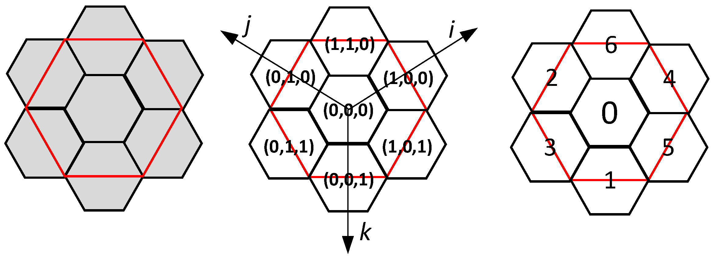
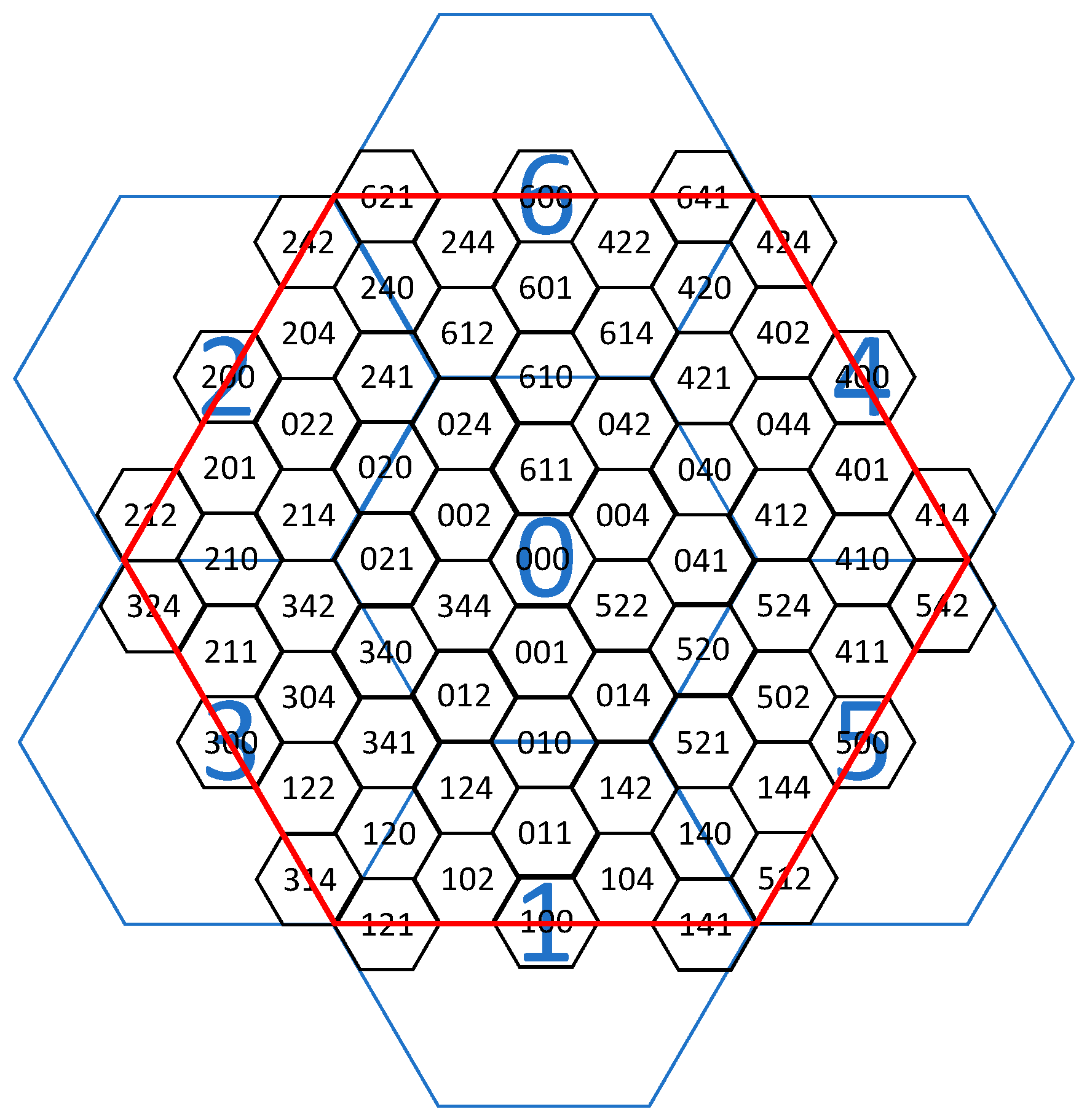
Degenerate Subdivision

Generally, people’s understanding of three-dimensional space is the Euclidean space defined by three orthogonal coordinate axes, such as a cube. By regularly dividing the space along each coordinate axis, the regular subdivision of the entire three-dimensional space can be achieved, and the distribution of the subdivision units in the three spatial dimensions is uniform and consistent.

The Earth’s layered space is not a Euclidean space, and geometrically, the two are not homeomorphic. If we follow the idea of uniform subdivision in the Euclidean three-dimensional space, we will face the problem of a large disparity in the granularity of the grid units; that is, the closer to the Earth’s center, the smaller the volume of the grid units and the denser the spatial distribution; the farther from the Earth’s center, the larger the volume of the grid units and the sparser the spatial distribution. In order to avoid this centripetal convergence effect of the grid units in spatial distribution, the design of the layered spatial grid takes into account the degenerate processing of the grid units. That is, in the hierarchical subdivision of the Earth’s layered space, among the sub-layer bodies subdivided from the same layer body, multiple sub-layer bodies close to the Earth’s center will be “merged” and thus “degenerate” into one sub-layer body. The result of the degenerate subdivision of the layered spatial grid is that the granularity of the layered spatial grid units and their distribution in the Earth’s space are more uniform.

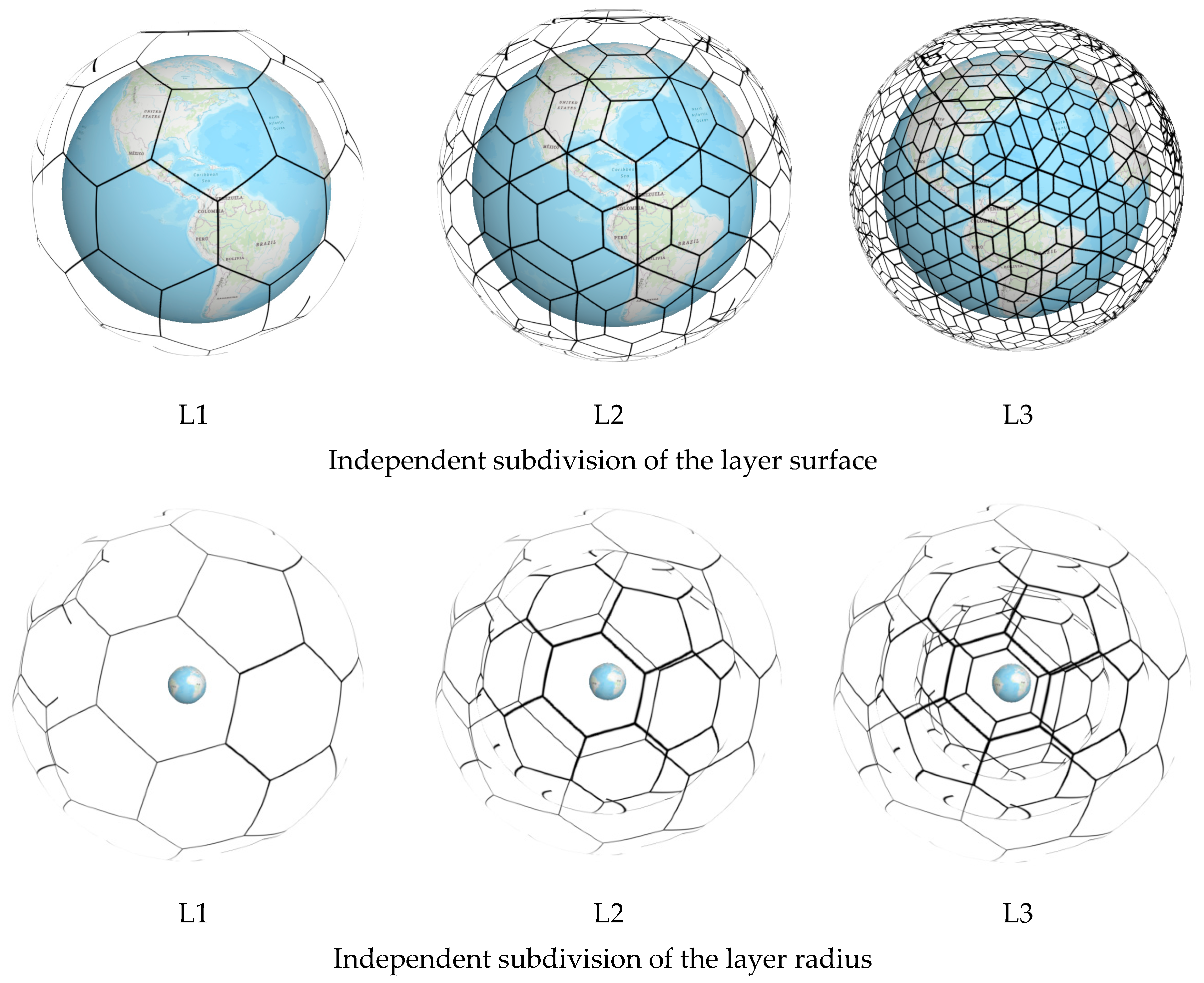
2.2.4. Subdivision Model of the Layer Surface of the ISEA4H-ESSG Temporal and Spatial Grid of the Earth System’s Layers

ISEA4H uses a regular icosahedron to fit the Earth’s surface and establishes a subdivision model on the surface of the regular icosahedron. The following figure is a schematic diagram of the regular icosahedron used to fit the Earth’s surface when it is unfolded on a spherical surface. A regular icosahedron has twenty regular triangles, which can be divided into twenty complete ground hexagonal tiles on the triangular surfaces and corner-missing hexagonal tiles composed of twelve vertex triangles, as shown in Figure 4.

In the global grid, the subdivision apertures are based on the hexagonal ones, including the three-aperture, four-aperture, and seven-aperture, and there are four commonly used hexagonal subdivision structures, as shown in Figure 5. The red hexagon representing the parent unit is subdivided into several black hexagons representing the sub-units. (a) is the three-aperture subdivision structure, (b) and (c) are the four-aperture subdivision structures, and (d) is the seven-aperture subdivision structure. Among them, there is a problem of direction transformation in the seven-aperture subdivision, which affects the efficiency of the grid-coding operation. However, the four-aperture hexagonal subdivision is relatively simple and convenient for coding operations.

According to this subdivision structure, the subdivision structure shown in the figure is formed on each triangular surface, and based on this rule, recursive hierarchical subdivision is carried out to generate higher-level grid units, as shown in Figure 6.

The planar hexagonal grid subdivision results generated can be used to generate a spherical hexagonal grid spherical model through the inverse ISEA projection, as shown in the figure. The lines formed by the boundaries of these spherical hexagons divide the Earth’s surface into various spatial subdivision curves with equal areas. The spherical grid formed by using these subdivision curves does not have the problem of polar oscillation, and the grid units are evenly distributed on the global surface. Moreover, the grid on the spherical surface has the characteristic of infinite subdivision, enabling the acquisition of grids at any granular scale through subdivision. The global subdivision result at the third level is shown in Figure 7.

2.2.5. The ISEA4H-ESSG Layered Block Subdivision Model of the Earth-System Spatiotemporal Grid

The subdivision of the three-dimensional space of the Earth’s layers is carried out in two directions: the layer surface and the layer radius. The single spherical surface obtained from the hexagonal grid subdivision based on the regular icosahedron can serve as the subdivision surface for the radial subdivision of the Earth’s space. After dividing the three-dimensional space of the Earth’s layers into several reference layer bodies, the spatial subdivision will be carried out around the hierarchical subdivision of the near-Earth layer surface. The three-dimensional space of the Earth’s layers is divided into a series of spatial units by using the subdivision surface, which can be called subdivision block elements. The geometric structure of each subdivision block element can be described as: V{S, E, P}, where V represents the layer body, S represents the surface of the layer body, E represents the edges of the layer body, and P represents the faces of the layer body. Any subdivision block is composed of 12 vertices, 18 edges, and 8 faces.

As shown in Figure 8, it is the division of each layer of the Earth. The layer body that this study focuses on is the near-Earth space layer, that is, the layer within the height from the Earth’s surface to the low-orbit satellites, which can be regarded as a spherical shell with a certain thickness. The division of the reference layer bodies is based on the layered structure of the Earth system and the characteristics of human activities in each layer. Through the reference layer bodies, the division range of the layered spatial grid can be defined, and the hierarchical subdivision of the layered spatial grid can be made more in line with the needs of modeling and analysis in a specific layered space.

According to the specific modeling needs, setting the reference layer body is actually an expansion of the division of the reference layer bodies. The reference layer body can be regarded as a finer layered structure. For example, reference layer bodies are set up for the stratosphere and troposphere of the atmosphere layer. In this way, the spatial distribution of the grid units in the layered space can be closer to the requirements of the specific modeling space.

For the spherical shell between the reference layer body and the target layer body, a radial subdivision model is established. Influenced by the regular subdivision mechanism of SDOG (Degenerate Quadtree Grid), a radial regular subdivision model is established.

For the Earth system, the subdivision is carried out by using the independent subdivision methods of the layer radius and the layer surface. The independent subdivision of the layer radius means that the layer radius is subdivided relatively until it meets specific requirements, and the grid of the layer surface remains unchanged during this process. The independent subdivision of the layer surface means that the layer surface of each layer’s spherical shell is subdivided until it meets specific requirements, and the division of the layer radius remains unchanged during this process. Different subdivided-unit spherical shells on the layer radius can obtain the scale closest to the specific requirements according to the rules of spherical subdivision, and the grids on each spherical surface and the grids on the edges of each layer body radius can be infinitely subdivided, respectively. In the scientific research of the Earth system, data with uneven spatial sampling are often used, such as NCEP FNL, which includes parameters such as vertical velocity and temperature. The resolution of these data in the radial direction of the Earth is 0.1–0.5 km, and the resolution on the spherical surface is 110 km–110 km (close to 1° × 1°). For this kind of data with uneven spatial sampling, the grids with independent radial and spherical subdivision can meet their granularity requirements, as shown in Figure 9.

When designing the independent subdivision of the layer radius/layer surface, the geometric indicators that generally should be considered are the differences in the granularity of spatial data sampling and the granularity of spatial modeling units in the Earth’s radial direction and on the spherical surface. For example, it is required that the volumes of the layer body units at the same level are approximately equal, or that the length ratio of the longitude edges to the radial edges (latitude edges to the radial edges) of the layer-body units at the same level is close to a given value. The modeling result of the third layer of the layer body is shown in Figure 10.

2.3. Encoding of the Temporal and Spatial Grid of the Earth System’s Layers

Grid encoding mainly solves the problem of uniquely identifying any grid unit; that is, the position identification of the grid unit. The spatial grid encoding model is actually an algebraic system of the spatial subdivision model, establishing the algebraic relationship of spatial subdivision. For the same grid subdivision model, multiple encoding structures and methods can be designed, but the subdivision rules they reflect are consistent. The content of grid encoding includes the composition structure of grid encoding, the conversion relationship between grid encoding and spatial coordinates, and the spatial operations of grid encoding, etc. Generally speaking, the design of the grid encoding structure is based on the rules of grid spatial subdivision to reflect the difficulty, order, and number of spatial subdivision operations. The encoding of each grid unit corresponds to its geographical spatial range, and there is a conversion relationship between the two, namely encoding and decoding. The spatial operations of grid encoding mainly include the calculation of grid units under measurements such as distance, direction, and range. For example, querying the grid units within a given distance (searching for adjacent grid units is a special case of it), determining the directional relationship between grid units, and the grid units within a certain range.

2.3.1. ISEA4H-ESSG Encoding Structure

Generally, the grid space is regarded as a discretized (digitized) abstraction of the geographical space, and the digital grid unit encoding is used to replace the geographical space coordinates. Therefore, the grid encoding space is also called the digital space [33]. The basis for constructing the digital space of the layered spatial grid is the grid encoding structure and method of the layer-body units. The encoding of the layered spatial grid is established according to the spatial subdivision model of the layered spatial grid. To establish the digital space of the spatial grid, it is first necessary to formally describe the identification of the grid units. The formal description of the identification of the layered spatial grid units can be considered from different perspectives. From the perspective of the grid hierarchical subdivision process, the identifications of the five parts, namely the reference layer body, the subdivision level of the layer surface, the subdivision level of the layer radius, the layer radius unit, and the layer cell unit, are the basic parameters for uniquely determining any layer-body unit.

• Encoding of the Layer Surface

The encoding of the layer surface follows the structure of the Octagonal Hierarchical Quadtree Structure (OHQS) of the four-aperture hexagon based on the regular icosahedron. A hexagonal three-axis coordinate system (coordinate system) is adopted to describe and locate each hexagonal grid. The origin of the hexagonal three-axis coordinate system is located at the center point of the initial hexagon. The angles between the three coordinate axes are all 120 degrees, and they are perpendicular to the upper right side, the upper left side, and the bottom side of the hexagon, respectively, as shown in Figure 11. The grid coordinates of each quadrant are determined by two adjacent coordinate axes, and the value of the other coordinate axis is 0.

Note: The numbers in the figure are the hexagonal three-axis coordinates $(i,j,k)$ corresponding to the grids of the 1st, 2nd, and 3rd layers, corresponding to the three coordinate axes of $i$, $j$, $k$, respectively; the red hexagon is the initial hexagon.

The units of the hexagonal three-axis coordinate systems of the grids at each layer are all different. The basic units $\left({ui}_n,{uj}_n,{uk}_n\right)$ of the three coordinate axes of $i,j,k$, satisfying the following formula of the grid coordinate system at the layer:

$$\left\{\begin{array}{c}\left({ui}_{n-1},{uj}_{n-1},{uk}_{n-1}\right)=\left({\displaystyle \frac{1}{2}}{ui}_n,{\displaystyle \frac{1}{2}}{uj}_n,{\displaystyle \frac{1}{2}}{uk}_n\right)\\ \left({ui}_n,{uj}_n,{uk}_n\right)=\left({\displaystyle \frac{\sqrt{3}}{2^n}}L,{\displaystyle \frac{\sqrt{3}}{2^n}}L,{\displaystyle \frac{\sqrt{3}}{2^n}}L\right)\end{array}\right.,$$

(1)

In the formula: ${ui}_n,{uj}_n,{uk}_n$ and ${ui}_{n-1},{uj}_{n-1},{uk}_{n-1}$ are, respectively, the basic coordinate units of the three coordinate axes of i, j, k and of the grid at the $\mathrm{n}$th layer and the $n-1$th layer, and $L$ is the side length of the initial hexagon in Figure 11.

Since the four-aperture hexagonal grid cannot achieve a completely nested subdivision, in order to construct a subdivision encoding structure that can cover the initial hexagonal grid, this paper divides the encoding into the encoding of the first layer and the layer. Based on the corresponding relationship between the coordinates and the binary numbers of the encoding, the basic encoding structure of the four-aperture hexagon is constructed, which is convenient for realizing the efficient conversion between the encoding and the hexagonal three-axis coordinate system. Among them, for the coordinates of the grid in the first layer, starting from the i-axis and going counterclockwise, the corresponding binary numbers are {100, 110, 010, 011, 001, 101} in sequence, and the corresponding basic code elements are {4, 6, 2, 3, 1, 5}. The binary numbers in the directions of the i-axis, j-axis, and k-axis for the encoding of the layer are {100, 010, 001} in sequence, and the corresponding basic code elements are {4, 2, 1}, as shown in Figure 12 and

Table 2. Corresponding table of the encoding of the 2^nd to nth layers of the grid and the i, j, and k coordinates.

$(\mathit{i},\mathit{j},\mathit{k})$	$(0,\mathrm{0,0})$	$(0,\mathrm{0,1})$	$(0,\mathrm{1,0})$	$(1,\mathrm{0,0})$
Angle with the i-axis		$4\pi /3$	$2\pi /3$	0
Binary system	000	001	010	100
$a\_2~a\_n$	0	1	2	4

. Finally, the four-aperture hexagonal encoding shown in Figure 13 can be constructed.

Note: The red hexagon is the initial hexagon; the blue hexagons are the grid and encoding of the first layer; the black hexagons are the grid and encoding of the third layer.

2.

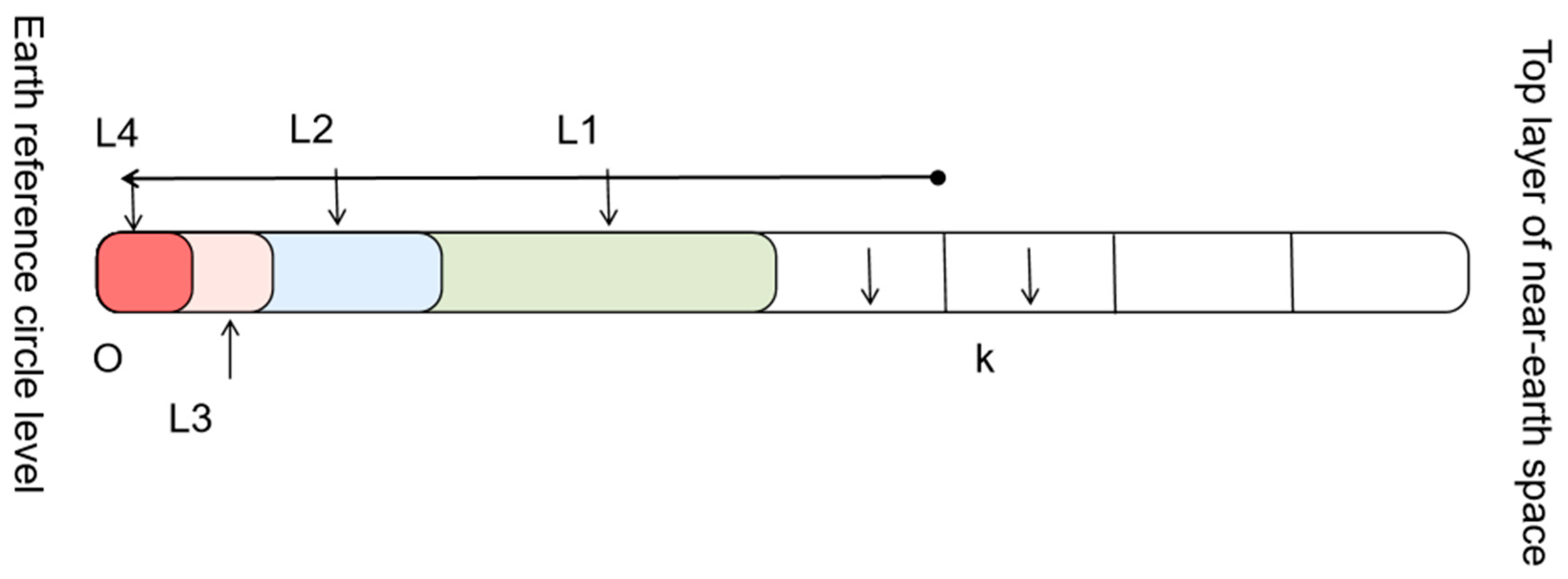
Encoding of the Layer Radius

The encoding of the layer radius is carried out only in a single direction. In the OHQS radial subdivision model, the layer radius direction adopts the rule of equidistant bisection for hierarchical subdivision. The encoding of each segment of the layer radius is described by its subdivision level (l) and its coordinate (k) on the radius of the layer body, in the form of l–k, where the starting point is the inner end point of the radius of the layer body.

According to the rule of equal division of the layer radius, in the l-th level of subdivision, the total number of segments of the layer body in the radial direction is $K=2^L$ for the layer radius; then, the encoding of each segment of the layer radius is 0 ≤ k ≤ K−1, as shown in Figure 14.

3.

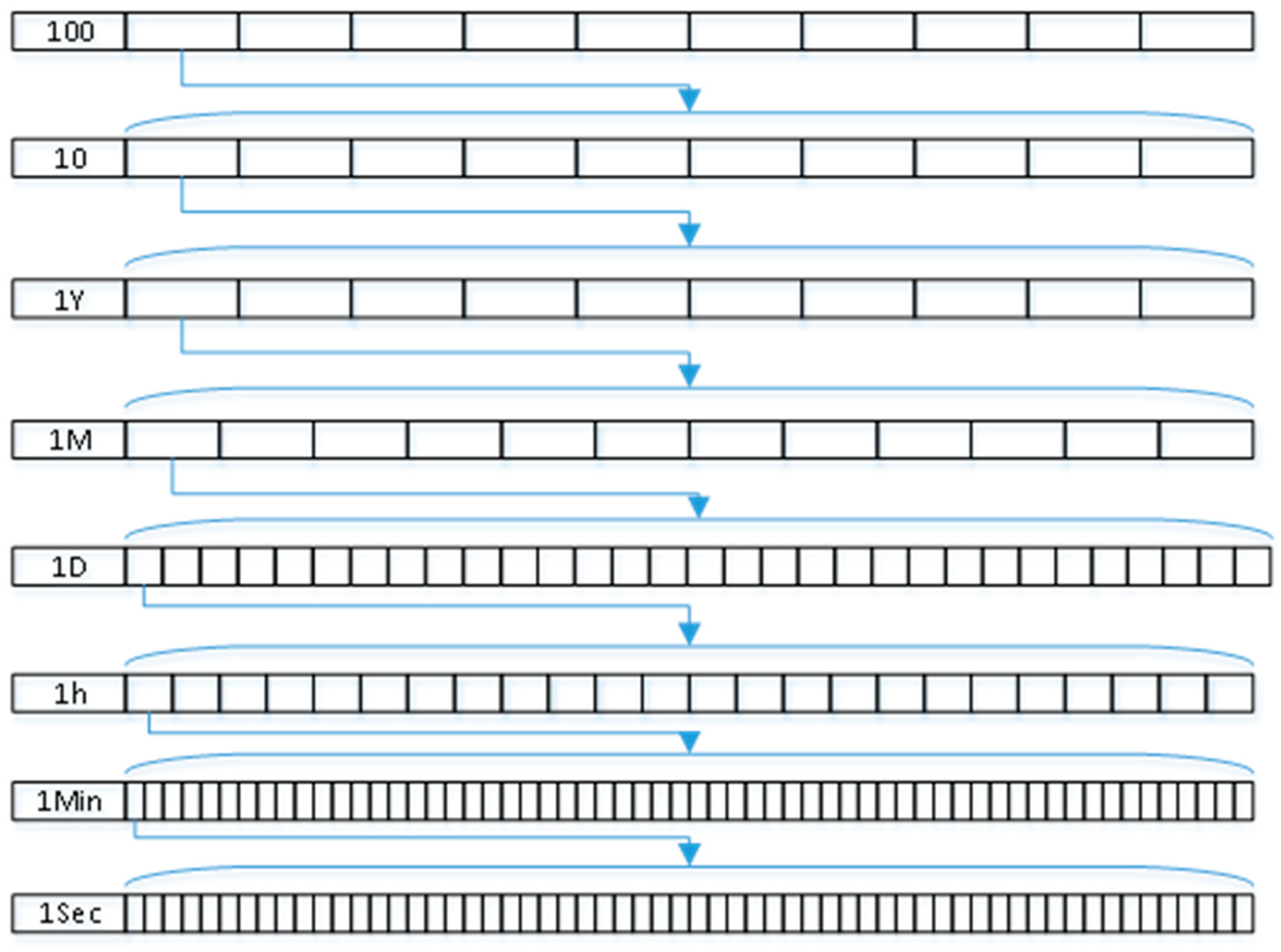
Temporal Subdivision and Encoding

Due to the characteristic of multi-temporal resolution of spatial data, this paper adopts a hierarchical subdivision scheme for temporal subdivision and encoding. Time is divided into different levels such as 100 years, 10 years, 1 year, 1 month, 1 day, 1 h, 1 min, and 1 s for subdivision, and unified encoding is carried out. The subdivision scheme and encoding are shown in Figure 14 and

Table 3. Encoding of temporal subdivision.

Temporal Resolution	Start Encoding	End Encoding
100 y	1	10
10	11	110
1 y	111	1110
1 m	1111	13110
1 d	13111	385110
1 h	385111	9313110
1 min	9313111	544993110
1 s	544993111	32685793110

. Finally, by combining the spatial data type, temporal encoding, and subdivided grid encoding, we can construct the spatiotemporal encoding scheme OHQS-ST for spatial data, integrating Optimized Hexagonal Quadtree Structure with spatiotemporal encoding, as shown in Figure 15.

2.3.2. Encoding Structure

The layer-body encoding is composed of temporal encoding, layer-surface encoding, and layer-radius encoding. The encoding method of OHQS is still used for the layered spatial grid on the layer surface. First, according to the Earth’s reference layer surface and the top layer surface of the near-Earth space, the Earth’s spatial layers are divided into the initial layer body (spherical shell), and then the initial layer body is continuously subdivided from two dimensions: the layer surface and the layer radius. The subdivision identification of the layer body should reflect the subdivision levels on the layer radius and the layer surface, as well as the number of a certain subdivision unit on the layer surface and the layer-radius surface. Among them, the numbering of the subdivision levels starts from 0 and increases sequentially; the number of a certain subdivision unit (i.e., the radius element) on the layer radius is numbered according to its sequence number in the total number of subdivision units of the layer radius at the current subdivision level, and the numbering order increases sequentially from the inside to the outside; the number of a certain subdivision unit (i.e., the layer cell) on the layer surface is consistent with the OHQS grid encoding, which is divided into (i, j, k) encoding.

The basic unit of encoding is the encoding component. According to the identification method of the subdivision of the layer body, the encoding components of the layer body include the number of the subdivision level of the layer radius, the number of the subdivision level of the layer surface, the number of the layer-surface unit, and the number of the layer-radius unit, as shown in

Table 4. Encoding structure of the layer body.

Composition of the Layer Body Encoding	Code Element of the Layer Body	Data Type
Subdivision identification of the layer body	Code of the layer-surface unit	String
	Code of the subdivision level of the layer radius	String
	Code of the layer-radius unit	String

.

The formal structure of the layer-body encoding (SolidCellCode) is as follows:

[Layer-Surface Unit Code]-[Layer-Radius Unit Code]-[Temporal Code]

DatumSphereTag is the identification of the reference layer body, and DatumSphereID is the number of the reference layer body.

The encoding structure combines spatial and temporal components:

Layer-Surface Encoding: Uses a hexagonal three-axis coordinate system (i, j, k) based on OHQS, with binary mapping (e.g., {100, 010, 001} → {4, 2, 1}).

Layer-Radius Encoding: Employs equidistant bisection (e.g., l–k format, where l is level, k is segment).

Temporal Encoding: Hierarchically subdivides time (e.g., 1 year → 111, 1 day → 13111).

Here is a coding case. For a point at (lat: 40° N, lon: 116° E, alt: 100 km, time: 2023-02-06 12:00:00):

Map to ISEA4H surface cell (e.g., level 3, code 421).

Radial segment (e.g., level 2, k = 3 → 2–3).

Add temporal code (e.g., 1 h → 385111).

Resulting code: [DatumSphereID]-421-2-3-385111.

3. Results and Discussion

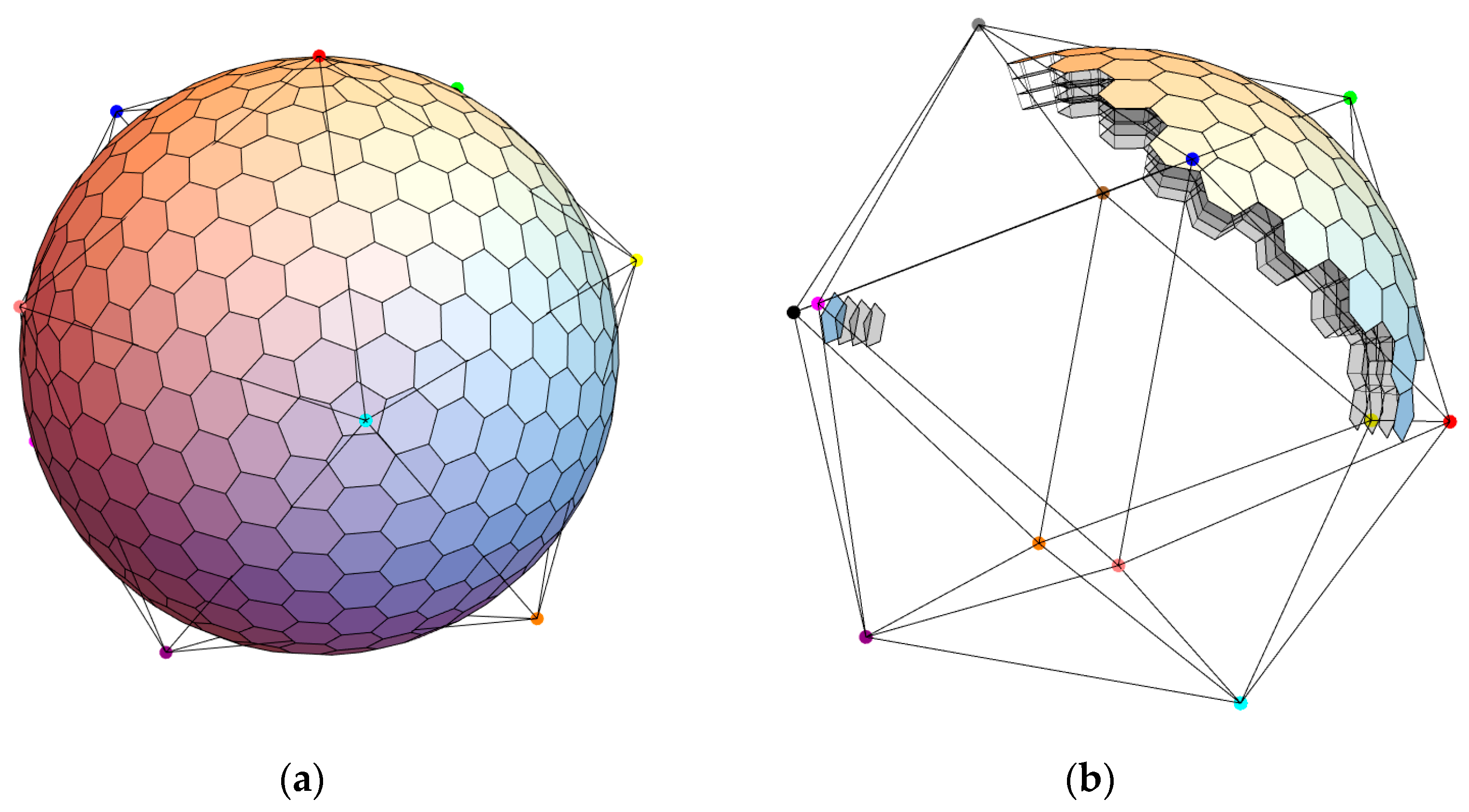
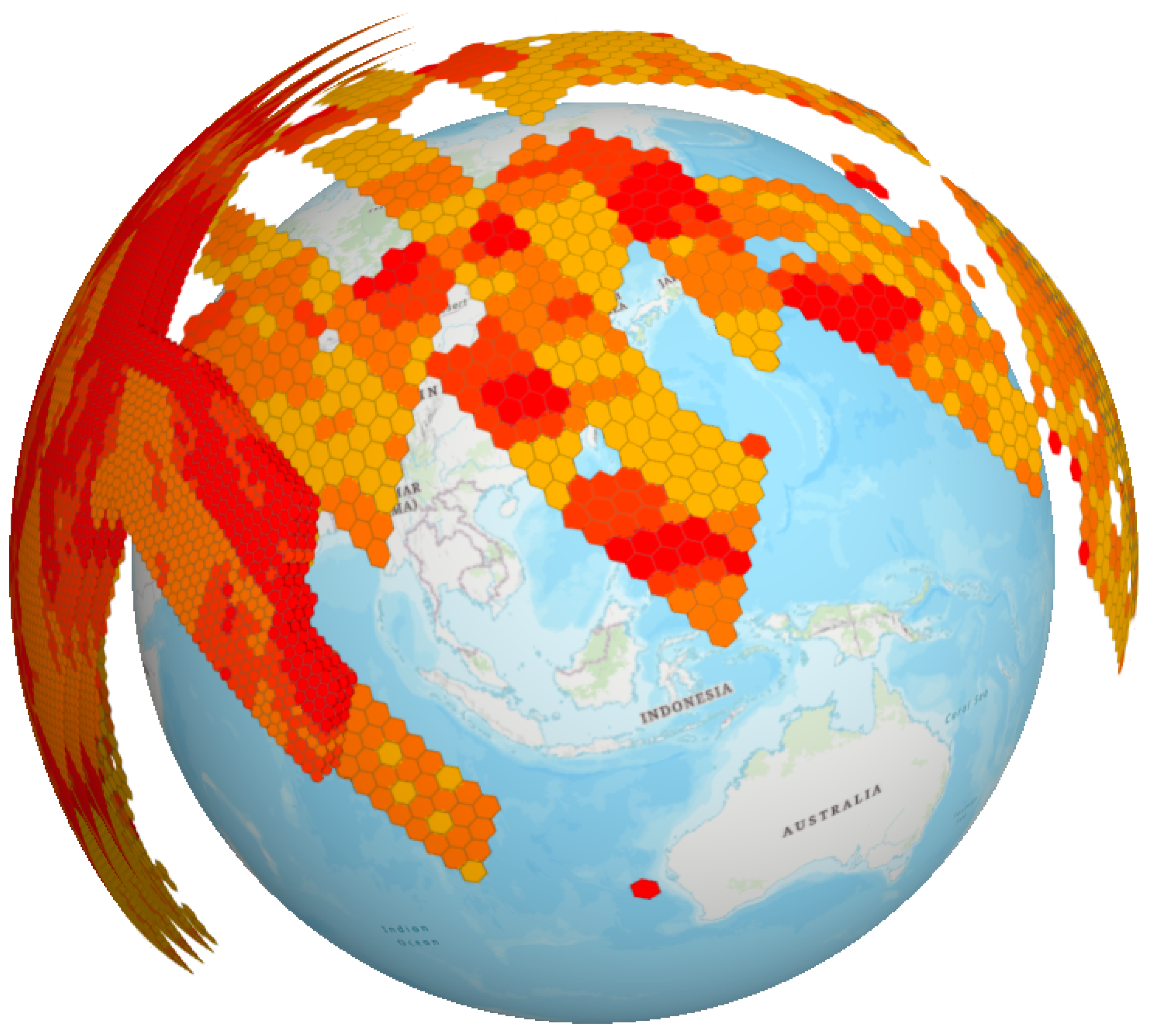
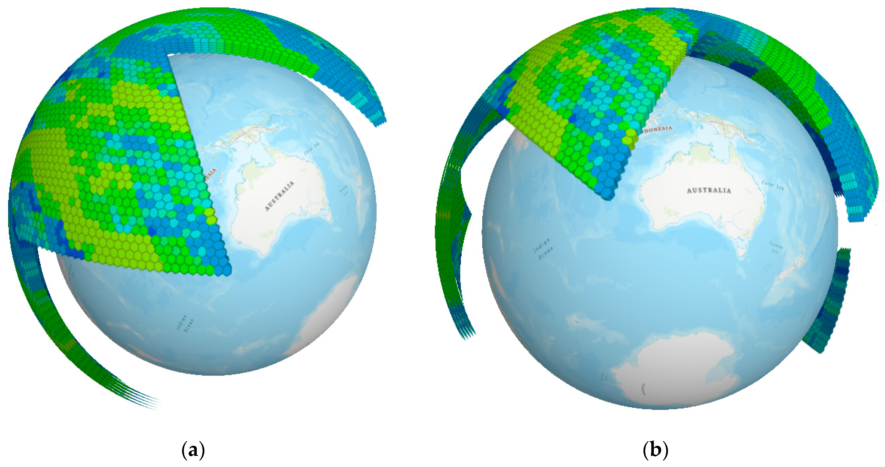
3.1. Three-Dimensional Modeling of the Ionosphere

In order to verify the applicability of the spatial grid of the Earth system for spatial data, the ionosphere is an important part of the near-Earth space environment. According to the IEEE standard, the ionosphere is defined as the entire space from an altitude of 60 km above the ground to the magnetopause. Affected by solar radiation, all molecules in this layer of space are ionized and mainly exist in the form of electrons or ions, which has an important impact on the propagation of electromagnetic waves, especially in fields such as satellite navigation, radio communication, space environment prediction, and spacecraft design (ISO 2009) [34]. The IRI (International Reference Ionosphere) ionosphere model is a global empirical ionosphere model established under the leadership of the Committee on Space Research (COSPAR) and the International Union of Radio Science (URSI) through long-term data observation. For any given time and spatial point, this model can provide parameters such as the global-monthly-average electron density, electron temperature, and ion temperature directly within the altitude range from 50 km to 2000 km (NASA) [35]. Electron density (Ne), that is, the number of free electrons per unit volume, is a very important parameter for describing the state of the ionosphere. It varies with changes in altitude, atmospheric composition, atmospheric density, and solar radiation flux, etc.

The data source of this study is the Global Navigation Satellite System—Total Electron Content (GNSS-TEC) database. These data contain GNSS observation data in the Receiver Independent Exchange (RINEX) format obtained from many regional GNSS receiver networks around the world. The dataset can be directly downloaded from https://stdb2.isee.nagoya-u.ac.jp/GPS/GPS-TEC/ (accessed on 11 March 2024). This precision aids satellite navigation by resolving vertical gradients missed by 2D grids, critical for GNSS accuracy. Software tools include Python 3.10 with NumPy for grid computation and ArcGIS Pro 3.0.1 for visualization. Steps: (1) Define reference layer surfaces; (2) apply ISEA4H subdivision; (3) implement radial splitting; (4) encode using OHQS v1. The experiment was conducted on a desktop (hardware environment: Intel Core i5-6500 CPU@3.20 GHZ, 16.0 GB RAM (Intel Corporation, Santa Clara, CA, USA), operating system: Windows 7).

The modeling results of this type of data in the grid of the Earth-system layers are shown in Figure 16.

In order to compare the retrieval efficiency of ISEA4H-ESSG with that of NetCDF (longitude and latitude grid) and H3 grid, 10,000 codes are randomly selected from the 5th floor to the 12th floor for neighborhood retrieval, and the retrieval time is tested. The comparative experiment was conducted on a desktop (hardware environment: Intel Core i5-6500 CPU@3.20 GHZ, 16.0 GB RAM, operating system: Windows 7). As shown in Figure 17, the retrieval efficiency of ISEA4H-ESSG is much higher than that of other commonly used grids.

3.2. Formatting of Mathematical Components

Atmospheric temperature affects the motion state of the atmosphere, the formation of clouds, and precipitation. It is one of the main controlling factors for the state and evolution of the climate system. Meanwhile, it also influences the growth of organisms on the land surface, and is one of the most basic characteristic parameters of the atmosphere. The three-dimensional modeling of the global atmospheric temperature field plays an important role in studying global climate change, the ecological environment, the growth of vegetation, etc.

The NCEP reanalysis data are released in quasi-real-time online by the National Centers for Environmental Prediction (NCEP) and the National Center for Atmospheric Research [36]. It contains data of more than 50 years. This dataset is obtained after carrying out quality control and assimilation processing on the observation data from the ground, ships, radiosondes, weather balloons, aircraft, satellites, etc. The National Centers for Environmental Prediction (NCEP) in the United States releases the global 1° × 1° atmospheric reanalysis data in GRIB format to the public every 6 h on average (https://psl.noaa.gov/data/gridded/data.ncep.reanalysis.html, accessed on 11 March 2024), which includes parameter data such as air temperature, humidity, wind direction, and aerosols. The atmospheric temperature data are one of the numerous parameters in the reanalysis data, and its vertical range is from 10 hPa to 1000 hPa. This precision aids satellite navigation by resolving vertical gradients missed by 2D grids, critical for GNSS accuracy.

This type of data includes parameters such as vertical velocity and temperature. Its resolution in the Earth’s radial direction is approximately 0.1 to 0.5 km, while the resolution on the spherical surface is approximately 110 km × 110 km (close to 1° × 1°).

According to the characteristics of the NCEP FNL data, it is necessary to first carry out the subdivision of the layer radius until the ratio of the side length of the layer-radius division unit to that of the initial layer cell is close to 0.5 km:110 km (that is, 1:220).

Let the subdivision level of the layer radius be n, then the length of the radial side d = D/2ⁿ. When the length of the radial side is approximately equal to the length of the latitude side b of the equator in the first-level layer cell, that is

$$d\approx b/220$$

where

$$b=2\pi R/4\times 2^1\approx 5009\mathrm{k}\mathrm{m}$$

Then, there is

$$n=5$$

Therefore, it is necessary to carry out the subdivision of the layer radius five times, and then carry out the hierarchical subdivision according to ISEA4H according to the resolution, as shown in Figure 18.

Based on the grid-data-accuracy evaluation index system [37] proposed by Ma et al., the accuracy of NCEP data before and after conversion is evaluated, and the information entropy index is 0.976, the pixel RMSE is 7.45, and the interactive information is 0.984. The data recombination accuracy is good.

4. Conclusions

This paper proposes a new spatial data organization model for the Earth system, namely the Earth-System Layered Grid (ISEA4H-ESSG). Its core is to achieve seamless coverage and the unified integration of data from multiple Earth layers (atmosphere, hydrosphere, lithosphere, near-Earth space, etc.) by constructing a global discrete three-dimensional grid system. Based on the ISEA4H subdivision model, ESSG breaks through the two-dimensional planar limitations of the traditional latitude and longitude grid and establishes a three-dimensional grid framework, solving the key bottlenecks in the modeling and analysis of cross-layer, multi-scale, and dynamic data. The main conclusions are as follows:

ESSG adheres to six core principles (three-dimensional layer coverage, geographical consistency, multi-scale dynamic adaptability, seamless division across the entire region, uniqueness and efficiency of encoding, and data-fusion compatibility). By integrating the icosahedron four-aperture hexagonal subdivision (ISEA4H) with the degenerated subdivision mechanism, it realizes the uniform discretization of the Earth’s three-dimensional space. Through the independent subdivision mechanisms of the layer surface and the layer radius, this model effectively balances the differences in spatial resolution between the spherical surface and the radial direction, and solves problems such as grid distortion in the polar regions and data heterogeneity across different layers. Experiments show that ESSG demonstrates high precision and adaptability in the modeling of ionospheric electron density and the three-dimensional reconstruction of the global atmospheric temperature field, verifying its ability to fuse data from multiple layers.

The uniqueness of the encoding and the hierarchical structure of ESSG significantly improve the storage and calculation efficiency of massive spatial data. Its compatibility framework supports the seamless integration of multi-source data (remote sensing, ground observation, simulation data). By introducing temporal subdivision encoding, the model is further expanded into a four-dimensional spatiotemporal framework, providing a new tool for the real-time monitoring and prediction of dynamic Earth-system processes (such as climate change and disaster evolution). In addition, the hexagonal grid characteristics of ESSG (equal area property, no directional preference) and its adaptability to the cloud-computing environment give it unique advantages in large-scale parallel computing and global environmental simulation. However, because its pixels and geometric structure are based on hexagonal cells, there are some difficulties in the compatibility of existing open-raster image files, and it is necessary to add some mappings to rectangular arrays.

The ESSG model provides a unified spatial data infrastructure for Earth-system science research. Its three-dimensional, multi-scale, and dynamically adaptable characteristics meet the urgent needs of global change research and sustainable development. ISEA4H-ESSG unifies multi-layer data with high precision and efficiency (20% faster retrieval than H3), despite higher setup costs. It excels in 3D modeling and data fusion, supporting all kinds of research on the Earth system, such as hazard and climate research. With the innovation of Earth observation technologies and the improvement of computing capabilities, ESSG is expected to become a core tool for connecting data from multiple layers and driving interdisciplinary innovation, providing scientific support for addressing global challenges such as climate change, disaster early warning, and space environment monitoring. Future research should focus on model optimization, technology integration, and standardized promotion to propel Earth-system science into a new stage of holography and intelligence, as well as optimizing encoding and enhancing cloud scalability.

References

1. Goodchild, M.F. Geographic information systems. In Research Methods in Geography; Gomez, B., Jones, J.P., III, Eds.; Wiley-Blackwell: Chichester, UK, 2010; pp. 376–391. [Google Scholar]
2. Pulinets, S.; Ouzounov, D. Lithosphere–Atmosphere–Ionosphere Coupling (LAIC) model–An unified concept for earthquake precursors validation. J. Asian Earth Sci. 2011, 41, 371–382. [Google Scholar]
3. Goodchild, M.F.; Guo, H.; Annoni, A.; Bian, L.; de Bie, K.; Campbell, F.; Craglia, M.; Ehlers, M.; van Genderen, J.; Jackson, D.; et al. Next-generation digital earth. Proc. Natl. Acad. Sci. USA 2012, 109, 11088–11094. [Google Scholar]
4. Barmin, I.V.; Kulagin, V.P.; Savinykh, V.P.; Tsvetkov, V.Y. Near-Earth space as an object of global monitoring. Sol. Syst. Res. 2014, 48, 531–535. [Google Scholar] [CrossRef]
5. Nwankwo, V.U.; Jibiri, N.N.; Kio, M.T. The impact of space radiation environment on satellites operation in near-Earth space. In Satellites Missions and Technologies for Geosciences; IntechOpen: London, UK, 2020; Volume 1, pp. 73–90. [Google Scholar]
6. Yu, J.; Wu, L.; Zi, G.; Guo, Z. SDOG-based multi-scale 3D modeling and visualization on global lithosphere. Sci. China Earth Sci. 2012, 55, 1012–1020. [Google Scholar]
7. Battrick, B. Global Earth Observation System of Systems GEOSS: 10-Year Implementation Plan Reference Document; Ad-Hoc Group on Earth Observations; Final Draft; ESA Publication Division: Noordwijk, The Netherlands, 2005. [Google Scholar]
8. Nativi, S.; Mazzetti, P.; Saarenmaa, H.; Kerr, J.; Tuama, É.Ó. Biodiversity and climate change use scenarios framework for the GEOSS interoperability pilot process. Ecol. Inform. 2009, 4, 23–33. [Google Scholar]
9. Bensana, E.; Lemaitre, M.; Verfaillie, G.J.C. Earth observation satellite management. Constraints 1999, 4, 293–299. [Google Scholar]
10. Sahr, K.; White, D.; Kimerling, A.J. Discrete Global Grid System. Cartogr. Geogr. Inf. Sci. 2003, 30, 121–134. [Google Scholar]
11. Yao, X.; Li, G.; Xia, J.; Ben, J.; Cao, Q.; Zhao, L.; Ma, Y.; Zhang, L.; Zhu, D. Enabling the Big Earth Observation Data via Cloud Computing and DGGS: Opportunities and Challenges. Remote Sens. 2019, 12, 62. [Google Scholar] [CrossRef]
12. Purss, M.B.J.; Gibb, R.; Samavati, F.; Peterson, P.; Ben, J. The OGC® Discrete Global Grid System core standard: A framework for rapid geospatial integration. In Proceedings of the 2016 IEEE International Geoscience and Remote Sensing Symposium (IGARSS), Beijing, China, 10–15 July 2016. [Google Scholar]
13. Goodchild, M.F. The Application of Advanced Information Technology in Assessing Environmental Impacts; Soil Science Society of America: Madison, WI, USA, 1996. [Google Scholar]
14. Goodchild, M.F.; Kimerling, A.J.E. Discrete Global Grids: A Web Book; National Center for Geographic Information and Analysis: New Yor, NY, USA, 2002. [Google Scholar]
15. Miliaresis, G.; Argialas, D. Segmentation of physiographic features from the global digital elevation model/GTOPO30. Comput. Geosci. 1999, 25, 715–728. [Google Scholar] [CrossRef]
16. Arabelos, D. Intercomparisons of the global DTMs ETOPO5, TerrainBase and JGP95E. Phys. Chem. Earth Part A Solid Earth Geodesy 2000, 25, 89–93. [Google Scholar]
17. Purss, M.B.; Peterson, P.R.; Strobl, P.; Dow, C.; Sabeur, Z.A.; Gibb, R.G.; Ben, J. Datacubes: A Discrete Global Grid Systems Perspective. Cartogr. Int. J. Geogr. Inf. Geovis. 2019, 54, 63–71. [Google Scholar]
18. Sun, W.; Cui, M.; Zhao, X.; Gao, Y. A global discrete grid modeling method based on the spherical degenerate quadtree. In Proceedings of the 2008 International Workshop on Education Technology and Training & 2008 International Workshop on Geoscience and Remote Sensing, Shanghai, China, 21–22 December 2008. [Google Scholar]
19. Dutton, G. Encoding and handling geospatial data with hierarchical triangular meshes. In Proceedings of the 7th International Symposium on Spatial Data Handling, Delft, The Netherlands, 12–16 August 1996. [Google Scholar]
20. Ottoson, P.; Hauska, H. Ellipsoidal quadtrees for indexing of global geographical data. Int. J. Geogr. Inf. Sci. 2002, 16, 213–226. [Google Scholar]
21. Gibb, R. The rHEALPix discrete global grid system. In IOP Conference Series: Earth and Environmental Science; IOP Publishing: Bristol, UK, 2016. [Google Scholar]
22. Zhao, L.; Li, G.; Yao, X.; Ma, Y.; Cao, Q. An optimized hexagonal quadtree encoding and operation scheme for icosahedral hexagonal discrete global grid systems. Int. J. Digit. Earth 2022, 15, 975–1000. [Google Scholar] [CrossRef]
23. Brodsky, I. H3: Uber’s Hexagonal Hierarchical Spatial Index. 2018. Available online: https://eng.uber.com/h3/ (accessed on 22 June 2019).
24. Ullrich, P.A.; Lauritzen, P.H.; Jablonowski, C. Geometrically Exact Conservative Remapping (GECoRe): Regular latitude–longitude and cubed-sphere grids. Mon. Weather. Rev. 2009, 137, 1721–1741. [Google Scholar] [CrossRef]
25. Béjar, R.; Lacasta, J.; Lopez-Pellicer, F.J.; Nogueras-Iso, J. Discrete Global Grid Systems with quadrangular cells as reference frameworks for the current generation of Earth observation data cubes. Environ. Model. Softw. 2023, 162, 105656. [Google Scholar]
26. Kageyama, A.; Sato, T.J.G. Geophysics, Geosystems, “Yin-Yang grid”: An overset grid in spherical geometry. Geochem. Geophys. Geosyst. 2004, 5. [Google Scholar] [CrossRef]
27. Bryan, G.L.; Norman, M.L.; O’Shea, B.W.; Abel, T.; Wise, J.H.; Turk, M.J.; Reynolds, D.R.; Collins, D.C.; Wang, P.; Skillman, S.W.; et al. Enzo: An adaptive mesh refinement code for astrophysics. Astrophys. J. Suppl. Ser. 2014, 211, 19. [Google Scholar]
28. Yu, J.; Wu, L.; Li, Z.; Li, X. An SDOG-based intrinsic method for three-dimensional modelling of large-scale spatial objects. Ann. GIS 2012, 18, 267–278. [Google Scholar]
29. Di, L.; Chen, A.; Yang, W.; Liu, Y.; Wei, Y.; Mehrotra, P.; Hu, C.; Williams, D. The development of a geospatial data Grid by integrating OGC Web services with Globus-based Grid technology. Concurr. Comput. Pract. Exp. 2008, 20, 1617–1635. [Google Scholar] [CrossRef]
30. Goodchild, M.F. Integrating GIS and remote sensing for vegetation analysis and modeling: Methodological issues. J. Veg. Sci. 1994, 5, 615–626. [Google Scholar]
31. Kimerling, J.A.; Sahr, K.; White, D.; Song, L. Comparing geometrical properties of global grids. Cartogr. Geogr. Inf. Sci. 1999, 26, 271–288. [Google Scholar]
32. Ben, J.; Tong, X.-C.; Zhang, Y.-S.; Zhang, H. Discrete global grid systems: Generating algorithm and software model. In Proceedings of the Geoinformatics 2006: Geospatial Information Technology, Wuhan, China, 28–29 October 2006. [Google Scholar]
33. Zhao, L.; Li, G.; Yao, X.; Ma, Y. Code Operation Scheme for the Icosahedral Hexagonal Discrete Global Grid System. Geo-Inf. Sci. 2023, 25, 239–251. [Google Scholar]
34. Fu, C.C.; Jhuang, H.K.; Ho, Y.Y.; Tsai, T.C.; Lee, L.C.; Lin, C.H.; Lin, C.R.; Walia, V.; Lee, I.T. A Study of Lithosphere–Ionosphere Seismic Precursors from Detecting Gamma-Ray and Total Electron Content Anomalies Prior to the 2018 ML6. 2 Hualien Earthquake in Eastern Taiwan. Remote Sens. 2025, 17, 188. [Google Scholar]
35. De Santis, A.; Jian, L.; Piersanti, M.; Shen, X.; Xiong, C.; Zhima, Z. Near-earth electromagnetic environment and natural hazards disturbances. Front. Environ. Sci. 2023, 11, 1307941. [Google Scholar]
36. Saha, S.; Moorthi, S.; Pan, H.-L.; Wu, X.; Wang, J.; Nadiga, S.; Tripp, P.; Kistler, R.; Woollen, J.; Behringer, D.; et al. The NCEP climate forecast system reanalysis. Bull. Am. Meteorol. Soc. 2010, 91, 1015–1058. [Google Scholar]
37. Ma, Y.; Li, G.; Yao, X.; Cao, Q.; Zhao, L.; Wang, S.; Zhang, L. A Precision Evaluation Index System for Remote Sensing Data Sampling Based on Hexagonal Discrete Grids. Int. J. Geo-Inf. 2021, 10, 194. [Google Scholar]
Figure 1. Classification system of global spatial grid.
Applsci 15 03703 g001
Figure 2. The layered structure characteristics of the Earth system.
Applsci 15 03703 g002
Figure 3. A conceptual diagram of the spatial grid of the Earth’s layers.
Applsci 15 03703 g003
Figure 4. An unfolded diagram of the regular icosahedron.
Applsci 15 03703 g004
Figure 5. Hexagonal subdivision apertures: (a) three-aperture (3 sub-units); (b) four-aperture type 1; (c) four-aperture type 2; (d) seven-aperture (7 sub-units). Black is the n+1th grid, and red is the nth grid.
Applsci 15 03703 g005
Figure 6. Iterative subdivision on the triangular surface: (a) describes the subdivision structures of the first and second layers, and (b) describes the hierarchical structures of the first, second, and third layers.
Applsci 15 03703 g006
Figure 7. The global subdivision result at the third level.
Applsci 15 03703 g007
Figure 8. The subdivision model of the layer radius.
Applsci 15 03703 g008
Figure 9. Independent subdivision of the layer surface and the layer radius.
Applsci 15 03703 g009
Figure 10. Visualization of the subdivision of the layer surface and layer body of the Earth-System Spatial Grid at the third layer. (a) shows the global grid at the third layer, and (b) shows the grid layers at the third layer of two adjacent triangular faces of the icosahedron.
Applsci 15 03703 g010
Figure 11. Hexagonal three-axis coordinate system at different grid levels.
Applsci 15 03703 g011
Figure 12. The encoding of the 2nd to nth layers of the four-aperture hexagonal grid.
Applsci 15 03703 g012
Figure 13. Four-aperture hexagonal coding.
Applsci 15 03703 g013
Figure 14. Encoding of the layer radius.
Applsci 15 03703 g014
Figure 15. Schematic diagram of temporal subdivision.
Applsci 15 03703 g015
Figure 16. A depiction of the hierarchical data of the ionospheric electron density TEC, with the data selected on 6 February 2023.
Applsci 15 03703 g016
Figure 17. Comparison of retrieval efficiency between H3, Jingwei grid and ISEA4H-ESSG.
Applsci 15 03703 g017
Figure 18. Three-dimensional modeling of the global atmospheric temperature field. (a,b) show different angles.
Applsci 15 03703 g018