
Bearing Lifespan Reliability Prediction Method Based on Multiscale Feature Extraction and Dual Attention Mechanism

Abstract
1. Introduction
- 1.
- A path weight selection mechanism was proposed, which could dynamically adjust the weights of feature paths according to different stages of bearing degradation, thereby capturing degradation information more accurately;
- 2.
- A dual attention mechanism was constructed, capable of flexibly capturing dependencies between channels and automatically adjusting the importance of each channel, which effectively enhanced the model’s feature representation capability;
- 3.
- The MS-DAN prediction method was proposed, which enhanced the feature extraction capability during the equipment degradation process and demonstrated excellent performance in prediction accuracy.
2. Materials and Methods
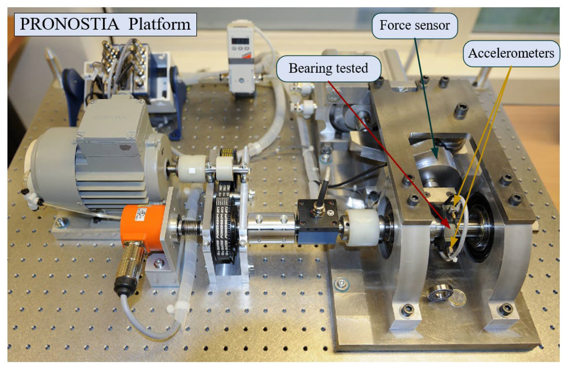
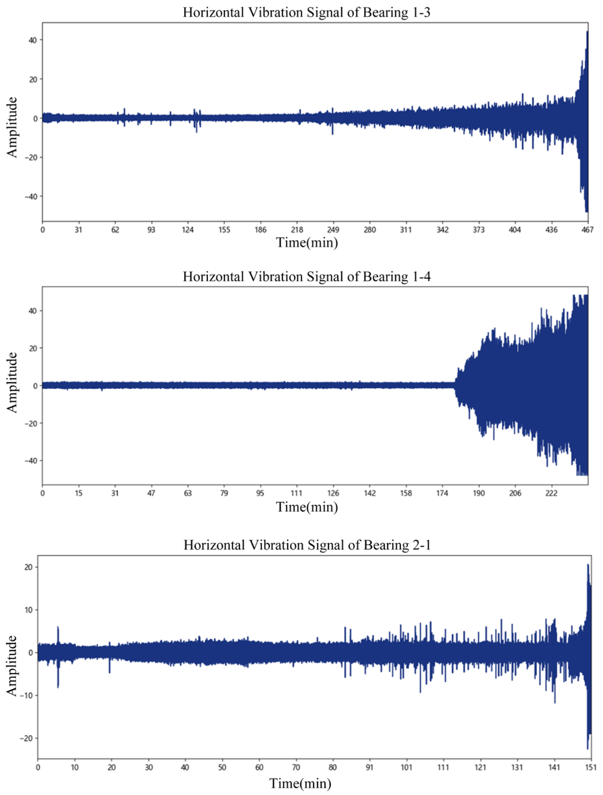
2.1. Materials
2.2. Methods
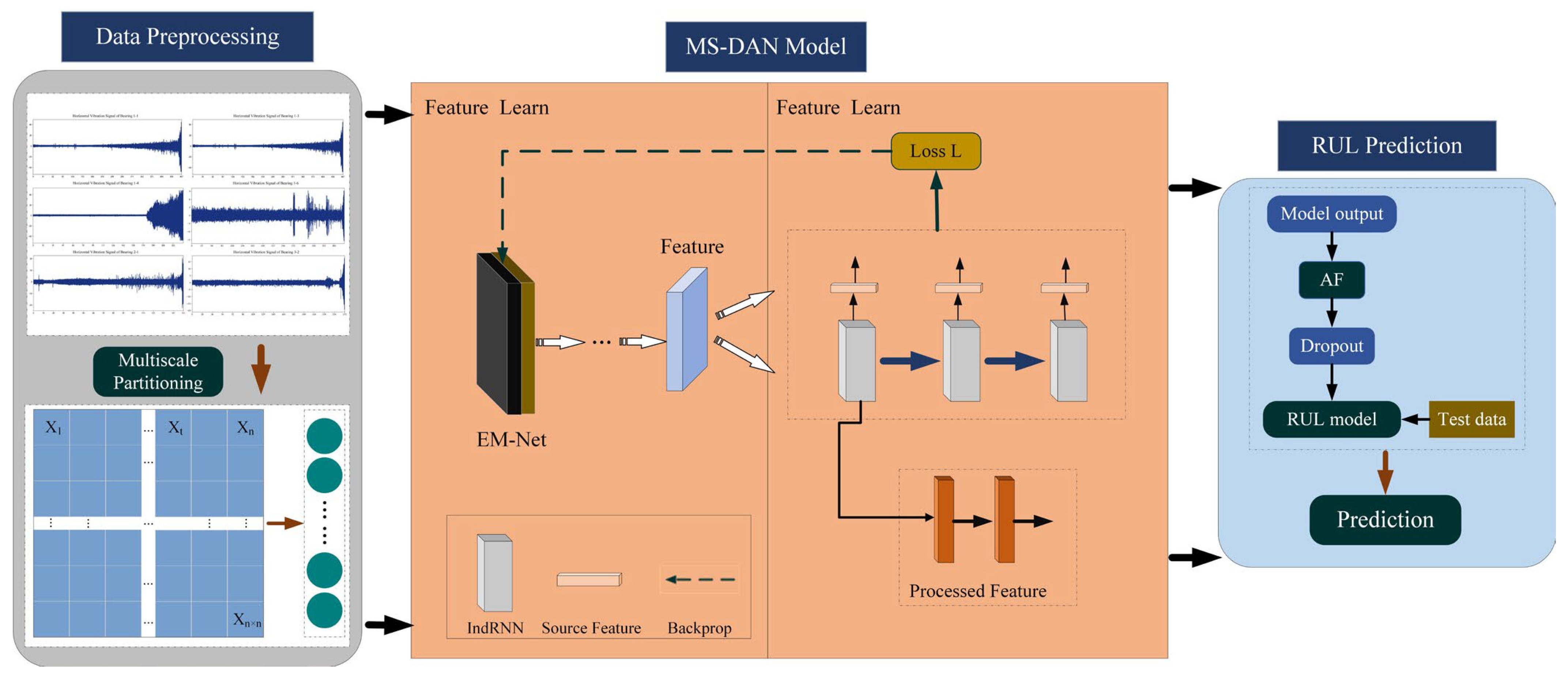
2.2.1. Overview
| Algorithm 1: Applying proposed to Prediction |
| Input: A set of dataset samples Learning_set = {(X1), (X2), …, (Xn)}. The Full_Test_Set is the test set. The number of learning epochs is M. Output: the optimal model and its predicted RUL
|
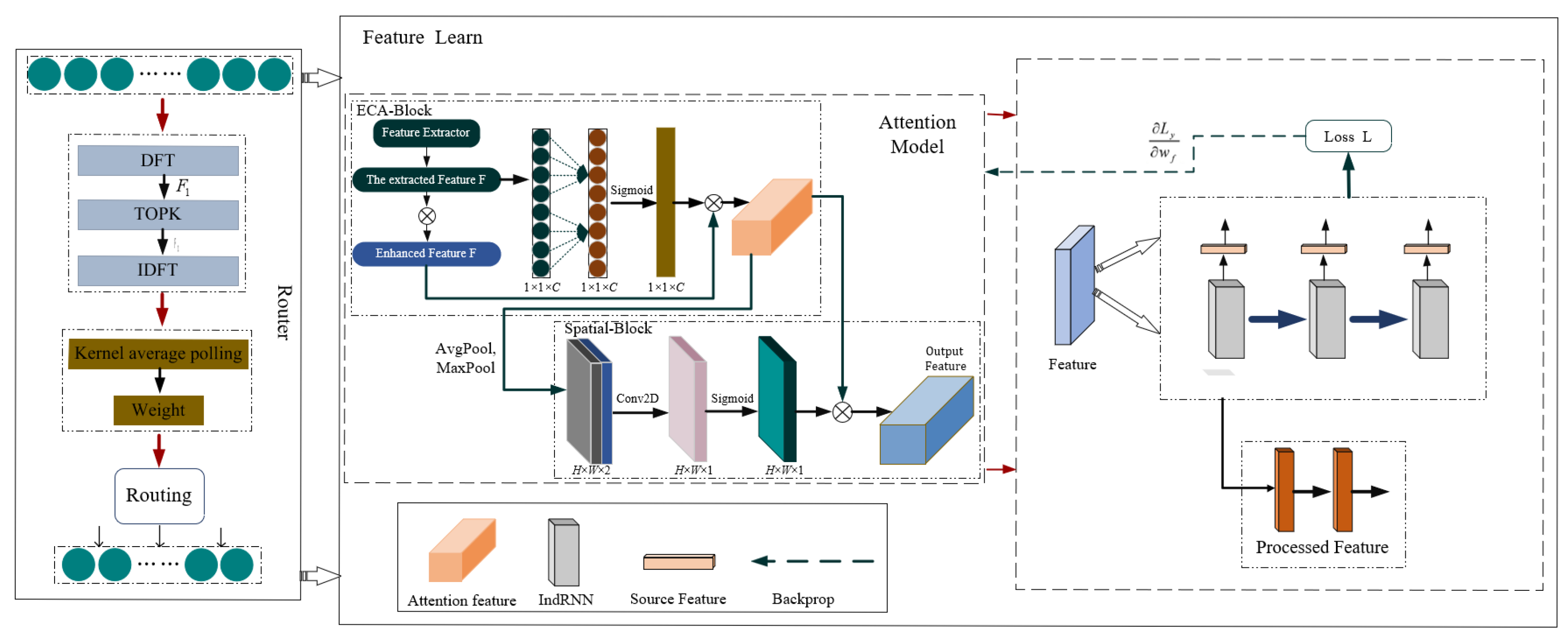
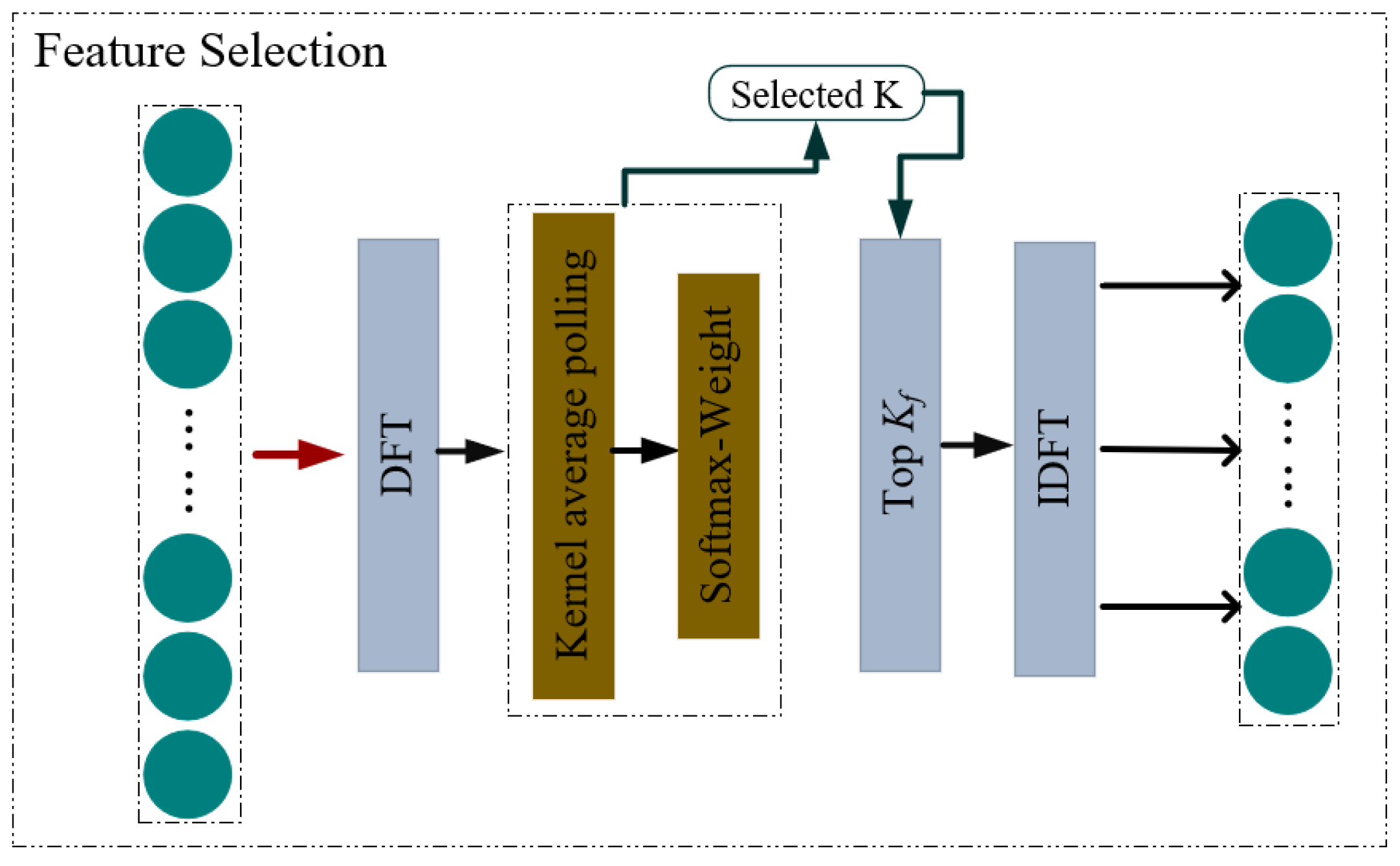
2.2.2. Multi-Scale Partitioning
| Algorithm 2: Feature Selection using DFT |
| Input: Time series X∈RH×d. Number of K. Output: Selected_k
|
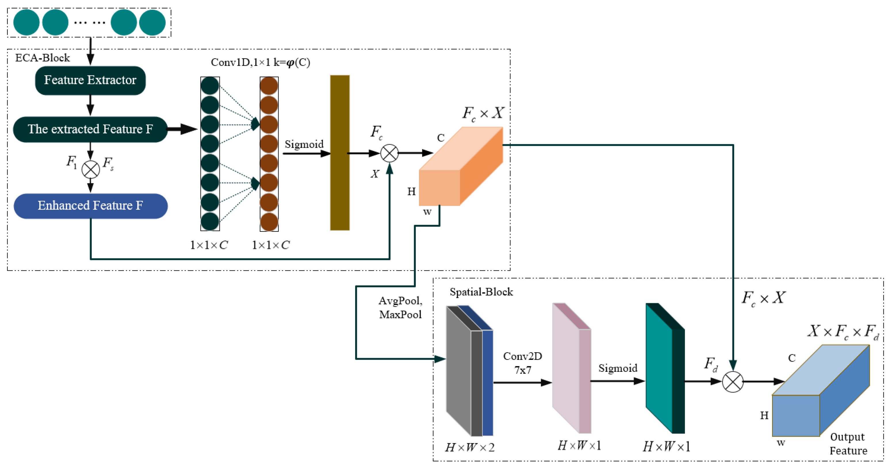
2.2.3. Attention Mechanism
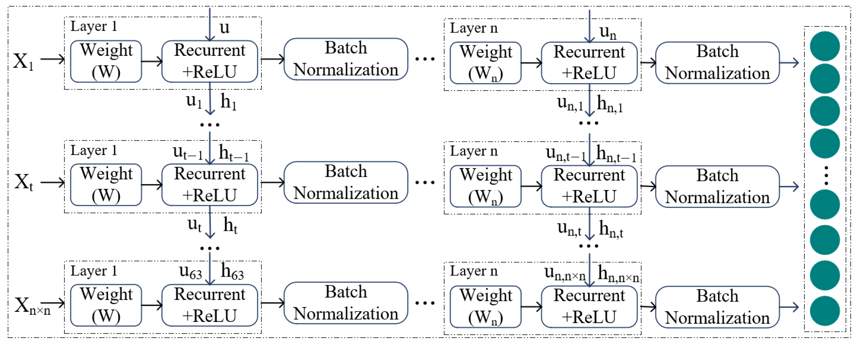
2.2.4. RNN
3. Results
3.1. Evaluation Criteria
3.2. Experimental Setup and Performance
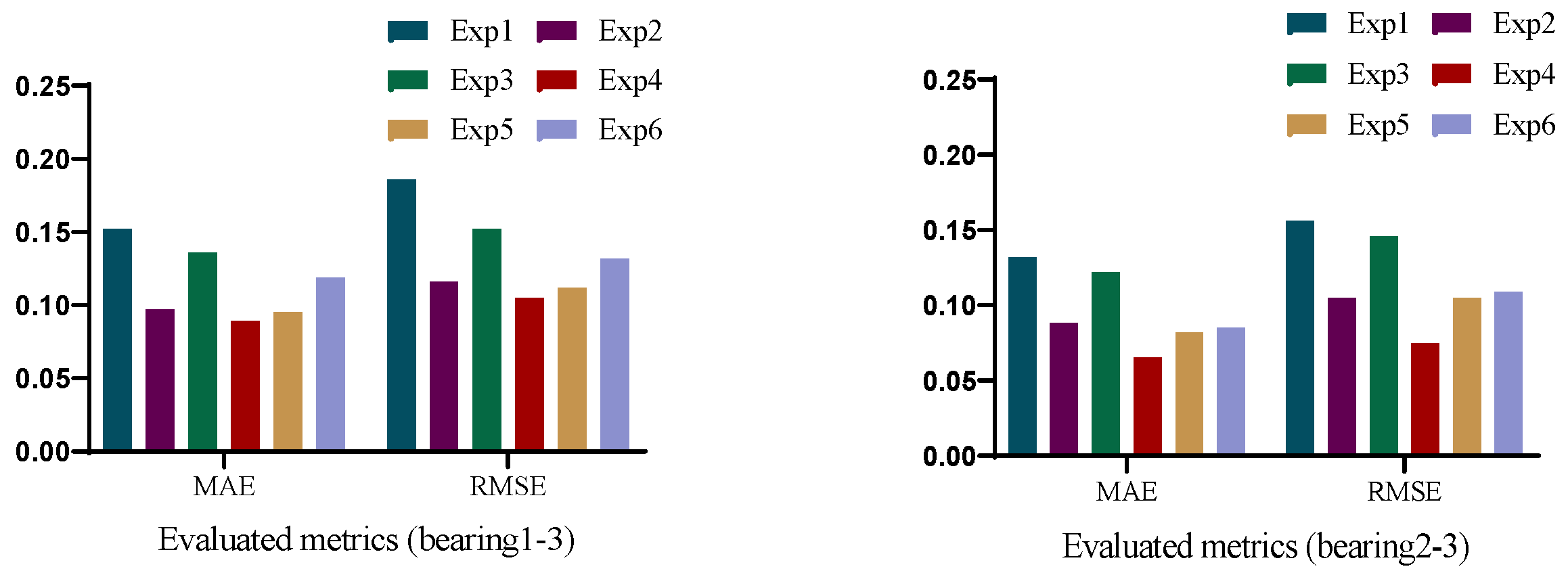
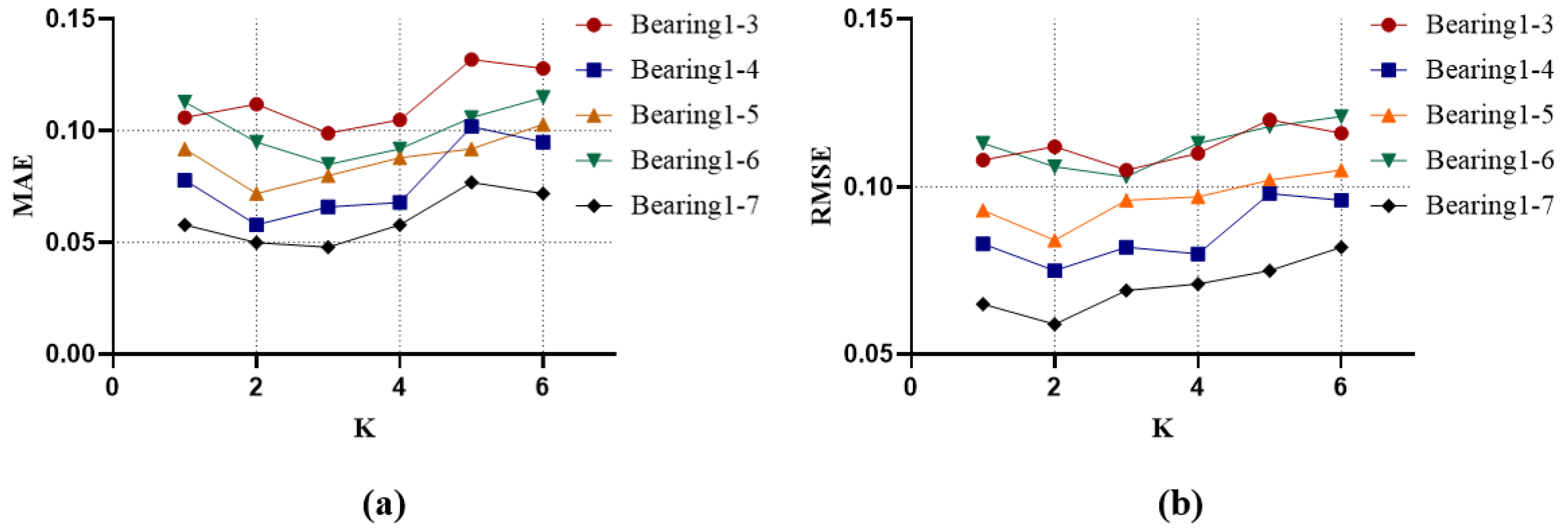
3.3. Ablation Experiment
3.4. Comparison of Different Modules
4. Discussion
5. Conclusions
Author Contributions
Funding
Institutional Review Board Statement
Informed Consent Statement
Data Availability Statement
Conflicts of Interest
Abbreviations
| MAE | Mean absolute error |
| RMSE | Root mean square error |
| RUL | Remaining useful life |
| LSTM | Long short-term memory |
| Bi-LSTM | Bidirectional long short-term memory |
| CNN | Convolutional neural network |
| TCN | Temporal convolutional network |
| DFT | Discrete Fourier Transform |
| RNN | Recurrent neural network |
| ECA-Net | Efficient channel attention network |
| CBAM | Convolutional block attention module |
| IndRNN | Independent recurrent neural network |
| GRU | Gated recurrent unit |
| BiGRU | Bidirectional gated recurrent unit |
References
- Wang, Y.; Zhao, Y.; Addepalli, S. Remaining useful life prediction using deep learning approaches: A review. Procedia Manuf. 2020, 49, 81–88. [Google Scholar]
- Ferreira, C.; Gonçalves, G. Remaining Useful Life prediction and challenges: A literature review on the use of Machine Learning Methods. J. Manuf. Syst. 2022, 63, 550–562. [Google Scholar]
- Zhang, Y.; Fang, L.; Qi, Z.; Deng, H. A review of remaining useful life prediction approaches for mechanical equipment. IEEE Sens. J. 2023, 23, 29991–30006. [Google Scholar]
- Zio, E. Some challenges and opportunities in reliability engineering. IEEE Trans. Reliab. 2016, 65, 1769–1782. [Google Scholar]
- Wang, Q.; Liu, W.; Xin, Z.; Yang, J.; Yuan, Q. Development and application of equipment maintenance and safety integrity management system. J. Loss Prev. Process Ind. 2011, 24, 321–332. [Google Scholar]
- Cepin, M.; Radim, B. Safety and Reliability. Theory and Applications; CRC Press: Boca Raton, FL, USA, 2017. [Google Scholar]
- Bagri, I.; Tahiry, K.; Hraiba, A.; Touil, A.; Mousrij, A. Vibration Signal Analysis for Intelligent Rotating Machinery Diagnosis and Prognosis: A Comprehensive Systematic Literature Review. Vibration 2024, 7, 1013–1062. [Google Scholar] [CrossRef]
- Zhang, P.; Chen, R.; Xu, X.; Yang, L.; Ran, M. Recent progress and prospective evaluation of fault diagnosis strategies for electrified drive powertrains: A comprehensive review. Measurement 2023, 222, 113711. [Google Scholar]
- Alyafeai, Z.; AlShaibani, M.S.; Ahmad, I. A survey on transfer learning in natural language processing. arXiv 2020, arXiv:2007.04239. [Google Scholar]
- Chai, J.; Zeng, H.; Li, A.; Ngai, E.W. Deep learning in computer vision: A critical review of emerging techniques and application scenarios. Mach. Learn. Appl. 2021, 6, 100134. [Google Scholar]
- Reza, M.; Mannan, M.; Mansor, M.; Ker, P.J.; Mahlia, T.M.I.; Hannan, M. Recent advancement of remaining useful life prediction of lithium-ion battery in electric vehicle applications: A review of modelling mechanisms, network configurations, factors, and outstanding issues. Energy Rep. 2024, 11, 4824–4848. [Google Scholar]
- Song, L.; Jin, Y.; Lin, T.; Zhao, S.; Wei, Z.; Wang, H. Remaining useful life prediction method based on the spatiotemporal graph and GCN nested parallel route model. IEEE Trans. Instrum. Meas. 2024, 73, 1–12. [Google Scholar]
- Gomez, W.; Wang, F.K.; Chou, J.H. Li-ion battery capacity prediction using improved temporal fusion transformer model. Energy 2024, 296, 131114. [Google Scholar]
- Hochreiter, S.; Schmidhuber, J. Long Short-term Memory. Neural Comput. 1997, 9, 1735–1780. [Google Scholar] [PubMed]
- Niazi, S.G.; Huang, T.; Zhou, H.; Bai, S.; Huang, H.-Z. Multi-scale time series analysis using TT-ConvLSTM technique for bearing remaining useful life prediction. Mech. Syst. Signal Process. 2024, 206, 110888. [Google Scholar]
- Vaswani, A.; Shazeer, N.; Parmar, N.; Uszkoreit, J.; Jones, L.; Gomez, A.N.; Gomez, Ł.; Polosukhin, I. Attention is all you need. Adv. Neural Inf. Process. Syst. 2017, 30. [Google Scholar] [CrossRef]
- Zhu, J.; Ma, J.; Wu, J. A regularized constrained two-stream convolution augmented transformer for aircraft engine remaining useful life prediction. Eng. Appl. Artif. Intell. 2024, 133, 108161. [Google Scholar]
- Lin, W.; Chai, Y.; Fan, L.; Zhang, K. Remaining useful life prediction using nonlinear multi-phase Wiener process and variational Bayesian approach. Reliab. Eng. Syst. Saf. 2024, 242, 109800. [Google Scholar]
- Kumar, A.; Parkash, C.; Vashishtha, G.; Tang, H.; Kundu, P.; Xiang, J. State-space modeling and novel entropy-based health indicator for dynamic degradation monitoring of rolling element bearing. Reliab. Eng. Syst. Saf. 2022, 221, 108356. [Google Scholar]
- Zhang, Q.; Liu, Q.; Ye, Q. An attention-based temporal convolutional network method for predicting remaining useful life of aero-engine. Eng. Appl. Artif. Intell. 2024, 127, 107241. [Google Scholar]
- Bai, S.; Kolter, J.Z.; Koltun, V. An empirical evaluation of generic convolutional and recurrent networks for sequence modeling. arXiv 2018, arXiv:1803.01271. [Google Scholar]
- Xu, D.; Xiao, X.; Liu, J.; Sui, S. Spatio-temporal degradation modeling and remaining useful life prediction under multiple operating conditions based on attention mechanism and deep learning. Reliab. Eng. Syst. Saf. 2023, 229, 108886. [Google Scholar]
- Ding, Y.; Jia, M. Convolutional transformer: An enhanced attention mechanism architecture for remaining useful life estimation of bearings. IEEE Trans. Instrum. Meas. 2022, 71, 3515010. [Google Scholar]
- Cai, Z.; Fan, Q.; Vasconcelos, N. A unified multi-scale deep convolutional neural network for fast object detection. In Proceedings of the 14th European Conference, Amsterdam, The Netherlands, 11–14 October 2016; Springer: Cham, Switzerland, 2016; Volume 14, pp. 354–370. [Google Scholar]
- Zhao, C.; Huang, X.; Li, Y.; Li, S. A novel remaining useful life prediction method based on gated attention mechanism capsule neural network. Measurement 2022, 189, 110637. [Google Scholar]
- Sabour, S.; Frosst, N.; Hinton, G.E. Dynamic routing between capsules. Adv. Neural Inf. Process. Syst. 2017, 30. [Google Scholar] [CrossRef]
- Wang, Z. Fast algorithms for the discrete W transform and for the discrete Fourier transform. IEEE Trans. Acoust. Speech Signal Process. 1984, 32, 803–816. [Google Scholar]
- Nie, Y.; Nguyen, N.H.; Sinthong, P.; Kalagnanam, J. A time series is worth 64 words: Long-term forecasting with transformers. arXiv 2022, arXiv:2211.14730. [Google Scholar]
- Elman, J.L. Finding structure in time. Cogn. Sci. 1990, 14, 179–211. [Google Scholar]
- Nectoux, P.; Gouriveau, R.; Medjaher, K. An experimental platform for bearings accelerated degradation tests. In Proceedings of the IEEE International Conference on Prognostics and Health Management IEEE, Beijing, China, 18–21 June 2012; pp. 23–25. [Google Scholar]
- Soualhi, A.; Medjaher, K.; Zerhouni, N. Bearing health monitoring based on Hilbert–Huang transform, support vector machine, and regression. IEEE Trans. Instrum. Meas. 2014, 64, 52–62. [Google Scholar]
- Singleton, R.K.; Strangas, E.G.; Aviyente, S. Extended Kalman filtering for remaining-useful-life estimation of bearings. IEEE Trans. Ind. Electron. 2014, 62, 1781–1790. [Google Scholar]
- Xu, L.; Huang, J.; Nitanda, A.; Asaoka, R.; Yamanishi, K. A Novel Global Spatial Attention Mechanism in Convolutional Neural Network for Medical Image Classification. arXiv 2020, arXiv:2007.15897. [Google Scholar]
- Wang, F.; Jiang, M.; Qian, C.; Yang, S.; Li, C.; Zhang, H.; Wang, X.; Tang, X. Residual Attention Network for Image Classification. In Proceedings of the IEEE Conference on Computer Vision and Pattern Recognition, Honolulu, HI, USA, 21–26 July 2017; pp. 3156–3164. [Google Scholar]
- Liu, C.; Huang, L.; Wei, Z.; Zhang, W. Subtler mixed attention network on fine-grained image classification. Appl. Intell. 2021, 51, 7903–7916. [Google Scholar]
- Wang, Q.; Wu, B.; Zhu, P.; Li, P.; Zuo, W.; Hu, Q. ECA-Net: Efficient Channel Attention for Deep Convolutional Neural Networks. In Proceedings of the Computer Vision and Pattern Recognition, Long Beach, CA, USA, 15–20 June 2019. [Google Scholar]
- Woo, S.; Park, J.; Lee, J.Y.; Kweon, I.S. Cbam: Convolutional block attention module. In Proceedings of the European Conference on Computer Vision, Munich, Germany, 8–14 September 2018; pp. 3–19. [Google Scholar]
- Shastry, K.A.; Shastry, A. An integrated deep learning and natural language processing approach for continuous remote monitoring in digital health. Decis. Anal. J. 2023, 8, 100301. [Google Scholar]
- Wei, D.; Wang, B.; Lin, G.; Liu, D.; Dong, Z.; Liu, H.; Liu, Y. Research on unstructured text data mining and fault classification based on RNN-LSTM with malfunction inspection report. Energies 2017, 10, 406. [Google Scholar] [CrossRef]
- Li, S.; Li, W.; Cook, C.; Zhu, C.; Gao, Y. Independently Recurrent Neural Network (IndRNN): Building A Longer and Deeper RNN. In Proceedings of the IEEE Conference on Computer Vision and Pattern Recognition, Salt Lake City, UT, USA, 18–22 June 2018. [Google Scholar]
- Zhao, B.; Li, S.; Gao, Y. IndRNN based long-term temporal recognition in the spatial and frequency domain. In Adjunct Proceedings of the 2020 ACM International Joint; Association for Computing Machinery: New York, NY, USA, 2020; pp. 368–372. [Google Scholar]
- Zhang, P.; Meng, J.; Luan, Y.; Liu, C. Plant miRNA-lncRNA Interaction Prediction with the Ensemble of CNN and IndRNN. Interdiscip. Sci. 2020, 12, 82–89. [Google Scholar] [PubMed]
- Liao, H. Image Classification Based on IndCRNN Module. In Proceedings of the ICVISP 2020: 2020 4th International Conference on Vision, Image and Signal Processing, Bangkok, Thailand, 9–11 December 2020; pp. 1–6. [Google Scholar]
- Pang, B.; Nijkamp, E.; Wu, Y.N. Deep learning with tensorflow: A review. J. Educ. Behav. Stat. 2020, 45, 227–248. [Google Scholar]
- Qiao, C.; Li, D.; Guo, Y.; Liu, C.; Jiang, T.; Dai, Q.; Li, D. Evaluation and development of deep neural networks for image super-resolution in optical microscopy. Nat. Methods 2021, 18, 194–202. [Google Scholar]
- Hodson, T. Root mean square error (RMSE) or mean absolute error (MAE): When to use them or not. Geosci. Model Dev. Discuss. 2022, 15, 5481–5487. [Google Scholar]
- Wei, G.; Zhao, J.; Feng, Y.; He, A.; Yu, J. A novel hybrid feature selection method based on dynamic feature importance. Appl. Soft Comput. 2020, 93, 106337. [Google Scholar]
- Shao, X.; Kim, C.-S. Adaptive multi-scale attention convolution neural network for cross-domain fault diagnosis. Expert Syst. Appl. 2024, 236, 121216. [Google Scholar]

| Operating Condition | Radial Force/N | Rotational Speed/(r·min⁻¹) | Training Set | Testing Set |
|---|---|---|---|---|
| Condition 1 | 4000 | 1800 | Bearing 1-1, Bearing 1-2 | Bearing 1-3, Bearing 1-4, Bearing 1-5, Bearing 1-6, Bearing 1-7 |
| Condition 2 | 4200 | 1650 | Bearing 2-1, Bearing 2-2 | Bearing 2-3, Bearing 2-4, Bearing 2-5, Bearing 2-6, Bearing 2-7 |
| Condition 3 | 4400 | 1500 | Bearing 3-1, Bearing 3-2 | Bearing 3-3 |
| Method | CNN | TCN | GRU | ||||
|---|---|---|---|---|---|---|---|
| Metric | MAE | RMSE | MAE | RMSE | MAE | RMSE | |
| Bearing 1 | 3 | 0.161 | 0.193 | 0.108 | 0.122 | 0.102 | 0.133 |
| 4 | 0.105 | 0.128 | 0.105 | 0.142 | 0.096 | 0.135 | |
| 5 | 0.162 | 0.193 | 0.185 | 0.251 | 0.153 | 0.228 | |
| 6 | 0.145 | 0.168 | 0.155 | 0.186 | 0.198 | 0.265 | |
| 7 | 0.125 | 0.149 | 0.172 | 0.256 | 0.182 | 0.236 | |
| Bearing 2 | 3 | 0.154 | 0.195 | 0.196 | 0.235 | 0.205 | 0.221 |
| 4 | 0.112 | 0.158 | 0.093 | 0.131 | 0.087 | 0.132 | |
| 5 | 0.151 | 0.186 | 0.189 | 0.215 | 0.191 | 0.238 | |
| 6 | 0.179 | 0.203 | 0.205 | 0.218 | 0.212 | 0.256 | |
| 7 | 0.184 | 0.216 | 0.195 | 0.232 | 0.196 | 0.245 | |
| Method | BiGRU | BiLSTM | Proposed (ours) | ||||
| Metric | MAE | RMSE | MAE | RMSE | MAE | RMSE | |
| Bearing 1 | 3 | 0.089 | 0.108 | 0.079 | 0.085 | 0.089 | 0.105 |
| 4 | 0.095 | 0.115 | 0.084 | 0.103 | 0.058 | 0.075 | |
| 5 | 0.128 | 0.156 | 0.106 | 0.132 | 0.072 | 0.084 | |
| 6 | 0.102 | 0.139 | 0.133 | 0.195 | 0.085 | 0.103 | |
| 7 | 0.106 | 0.122 | 0.085 | 0.105 | 0.048 | 0.059 | |
| Bearing 1 | 3 | 0.152 | 0.187 | 0.126 | 0.156 | 0.065 | 0.075 |
| 4 | 0.128 | 0.153 | 0.066 | 0.085 | 0.097 | 0.109 | |
| 5 | 0.151 | 0.208 | 0.132 | 0.166 | 0.080 | 0.098 | |
| 6 | 0.165 | 0.212 | 0.092 | 0.108 | 0.092 | 0.102 | |
| 7 | 0.159 | 0.195 | 0.132 | 0.176 | 0.112 | 0.119 | |
| Hyperparameters | Exp1 | Exp2 | Exp3 |
|---|---|---|---|
| Epochs | 50 | 50 | 50 |
| Batch size | 256 | 128 | 256 |
| optimizer | RMSprop | Adam | SGD |
| Learning rate | 10−3 | 10−3 | 10−3 |
| - | Exp4 | Exp5 | Exp6 |
| Epochs | 50 | 50 | 50 |
| Batch size | 256 | 128 | 256 |
| optimizer | Adam | Adam | Adam |
| Learning rate | 10−3 | 10−3 | 10−4 |
| Model | Evaluated Metrics | Bearing 1-5 | Bearing 2-3 | Bearing 2-5 |
|---|---|---|---|---|
| Base model | MAE | 0.128 | 0.121 | 0.133 |
| RMSE | 0.145 | 0.133 | 0.177 | |
| Base model + EM-NET | MAE | 0.093 | 0.081 | 0.103 |
| RMSE | 0.102 | 0.096 | 0.112 | |
| Ours (Base model + EM-NET + Multiscale) | MAE | 0.072 | 0.065 | 0.080 |
| RMSE | 0.084 | 0.075 | 0.098 |
| Methods | Evaluated Metrics | |
|---|---|---|
| MAE | RMSE | |
| TCN + Hybrid Attention Mechanism | 0.095 | 0.109 |
| Patch + PAS + Multiscale | 0.093 | 0.105 |
| DMW-Trans | 0.099 | 0.137 |
| MLP + Transformer | 0.111 | 0.140 |
| Ours | 0.089 | 0.105 |
Disclaimer/Publisher’s Note: The statements, opinions and data contained in all publications are solely those of the individual author(s) and contributor(s) and not of MDPI and/or the editor(s). MDPI and/or the editor(s) disclaim responsibility for any injury to people or property resulting from any ideas, methods, instructions or products referred to in the content. |
© 2025 by the authors. Licensee MDPI, Basel, Switzerland. This article is an open access article distributed under the terms and conditions of the Creative Commons Attribution (CC BY) license (https://creativecommons.org/licenses/by/4.0/).
Share and Cite
Luo, X.; Wang, M. Bearing Lifespan Reliability Prediction Method Based on Multiscale Feature Extraction and Dual Attention Mechanism. Appl. Sci. 2025, 15, 3662. https://doi.org/10.3390/app15073662
Luo X, Wang M. Bearing Lifespan Reliability Prediction Method Based on Multiscale Feature Extraction and Dual Attention Mechanism. Applied Sciences. 2025; 15(7):3662. https://doi.org/10.3390/app15073662
Chicago/Turabian StyleLuo, Xudong, and Minghui Wang. 2025. "Bearing Lifespan Reliability Prediction Method Based on Multiscale Feature Extraction and Dual Attention Mechanism" Applied Sciences 15, no. 7: 3662. https://doi.org/10.3390/app15073662
APA StyleLuo, X., & Wang, M. (2025). Bearing Lifespan Reliability Prediction Method Based on Multiscale Feature Extraction and Dual Attention Mechanism. Applied Sciences, 15(7), 3662. https://doi.org/10.3390/app15073662