Article

Wavelet Decomposition Prediction for Digital Predistortion of Wideband Power Amplifiers

School of Computer Science and Artificial Intelligence, Changzhou University, Changzhou 213164, China
*
Author to whom correspondence should be addressed.
Appl. Sci. 2025, 15(7), 3599; https://doi.org/10.3390/app15073599
Submission received: 20 February 2025 / Revised: 21 March 2025 / Accepted: 23 March 2025 / Published: 25 March 2025

Abstract

:
Digital predistortion (DPD) is essential for improving the efficiency and linearity of power amplifiers (PAs), particularly in radio frequency communication systems. We propose a wavelet decomposition prediction (WDP) framework that better adapts to the highly nonlinear characteristics of PAs. In this framework, the input data are first decomposed using wavelet transformation, allowing for a more effective representation of nonlinear features. Next, a nonlinear modeling process is conducted on the PA to capture its distortion characteristics. Once the nonlinear model is trained, it is frozen to preserve its learned features. Based on this frozen nonlinear model, DPD is then applied to the PA to compensate for nonlinear distortions. Experimental results demonstrate the effectiveness of our proposed method, achieving the best ACPR and EVM performance on the OpenDPD dataset.

1. Introduction

In modern communication systems, as transmission data rates and spectral efficiency continue to improve, nonlinear distortion has emerged as a critical factor impacting system performance. This distortion primarily originates from nonlinear components such as power amplifiers (PAs), which degrade signal quality, increase bit error rates, and introduce spectral pollution during transmission [1,2]. Ideally, a PA should exhibit linear behavior, maintaining a constant amplification factor between the input and output signals. However, during high-power operation, PAs inevitably deviate from their linear region, leading to the presence of nonlinear components in the output signal [3]. These nonlinear distortions not only compromise signal integrity but also introduce adjacent channel interference, further degrading overall system performance [4]. A conventional linearization approach is power back-off, which mitigates nonlinearity at the cost of significantly reducing PA efficiency and output power [5,6]. Consequently, PA design and optimization have long been key research topics in both academia and industry [7,8,9,10,11,12]. Among various linearization techniques, digital predistortion (DPD) is widely regarded as the most promising solution due to its flexibility and superior performance [13,14]. Due to its strong capability in fitting nonlinear characteristics, deep learning has emerged as a powerful tool in DPD research, driven by advancements in its techniques. Deep learning models, particularly neural networks, can effectively capture complex patterns and nonlinear dependencies from large datasets, enabling more precise predistortion. Therefore, in this study, we employ deep learning to model and optimize the DPD process.
Direct Learning Architecture (DLA) is a classic implementation method for predistortion techniques, whose core idea is to minimize the error between the PA output and the expected signal by directly optimizing the parameters of the predistorter. In DLA, the input signal is first processed by a predistorter to generate a predistorted signal, which is then amplified by the PA. Due to the nonlinear nature of PAs, the output signal may introduce distortion. DLA calculates the error signal by comparing the output signal of the PA with the original input signal and directly adjusts the parameters of the predistorter to minimize the error. Although DLA has the advantages of simple structure and easy implementation, its performance is limited by the complexity of inverse operations and model accuracy, especially in highly nonlinear systems, where DLA may face numerical instability and real-time challenges [15,16,17,18,19,20].
Different from DLA, Indirect Learning Architecture (ILA) is another classic method for implementing predistortion techniques, whose core idea is to indirectly model the characteristics of a PA and invert its inverse model to achieve predistortion. In ILA, the input signal first passes through the PA to generate an output signal containing nonlinear distortion. The input and output signals of the PA are used to train a forward model that characterizes the nonlinear characteristics of the PA. Subsequently, by inverting the forward model, the inverse model of the PA is obtained and used as a predistorter. Although ILA offers advantages such as model flexibility and indirect optimization, it suffers from several critical drawbacks, including vulnerability to noise due to parameter extraction at the PA output and high dependence on PA model accuracy, which may degrade predistortion performance [21,22,23,24].
Wavelet decomposition prediction (WDP) combines the strengths of both direct and indirect learning approaches, enabling the direct training of predistortion models without requiring model inversion after task completion. This method focuses on training a predistortion model within a nonlinear system, offering the advantage of directly computing predistortion coefficients. To accomplish this, WDP initially employs neural networks (NNs) to model the nonlinear behavior of the PA. Training is halted once the PA’s nonlinear model achieves a satisfactory level of accuracy. Subsequently, the parameters of this nonlinear model are copied to an identical model, which is then frozen. This frozen nonlinear model is cascaded with the predistorter, and by linearizing the output of the combined system, the objective of training an effective predistorter is realized [25,26,27].
In comparison to the ILA method, WDP offers improved robustness by avoiding reliance on the precise inversion of the PA model. In practical systems, the nonlinear characteristics of the PA can vary over time or with environmental changes, making accurate model inversion challenging and potentially degrading the performance of traditional ILA-based predistortion. In contrast, WDP employs neural networks to directly model the nonlinear behavior of the PA. Once trained, the model parameters are frozen, ensuring stability throughout the predistorter training process and enhancing overall system robustness.
Furthermore, compared to the DLA approach, which typically requires inverting the PA output to directly optimize the predistorter parameters, WDP also demonstrates advantages in stability and efficiency. The inversion process in DLA can become numerically unstable or computationally intensive in highly nonlinear systems. By avoiding such complex inverse operations and instead modeling PA nonlinearity through neural networks, WDP improves both system stability and computational efficiency.
However, existing WDP-based DPD methods often suffer from limited multi-resolution analysis capabilities and inadequate long-term dependency modeling, which significantly restricts their overall performance. To overcome these challenges, we introduce a novel WDP-based DPD approach that integrates dual-stage recurrent neural networks (RNNs) with wavelet decomposition (WD). The WD enhancement decomposes signals into low-frequency and high-frequency components, allowing the model to learn and distinguish different frequency features of the data more precisely and efficiently. This approach not only retains critical information but also improves the overall signal quality. By leveraging WD, the model gains a deeper understanding of the data’s intrinsic structure, enhancing its predictive accuracy and generalization capabilities in real-world applications. Specifically, we use a combination of WD and an update gate RNN (UGRNN) to model the nonlinearity of the PA, and the WD-enhanced framework enhances the model’s multi-resolution analysis capability. The UGRNN captures the long-term dependencies of decomposed signal components and introduces a self-attention mechanism to further evaluate the contribution of each component to the model output. In this stage, a normalized mean square error (NMSE) of 34.96 dB is achieved, which is superior to that of other methods. Subsequently, the UGRNN is replaced with an intersection RNN (IRNN) and cascaded with pretrained and frozen nonlinear models to linearize the output of the combined model and achieve effective DPD processing. Our proposed method provides excellent linearization performance on the open-source dataset ‘OpenDPD’, achieving adjacent channel power ratio (ACPR) of −52.71/−51.93 dBc and error vector magnitude (EVM) of −48.92 dB.
The contributions of this paper are summarized as follows.
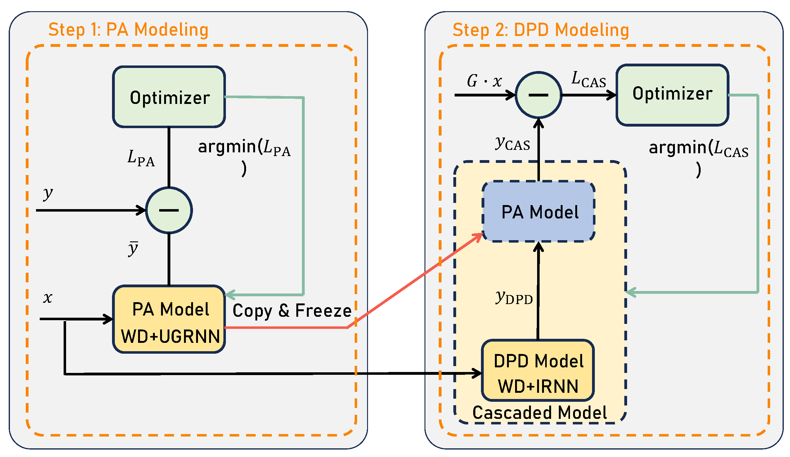
  • We propose a WD-enhanced dual-stage RNN for WDP-based DPD, where the dual-stage RNN captures long-term dependencies in the input while the WD module provides multi-resolution analysis, improving both PA modeling accuracy and DPD effectiveness.
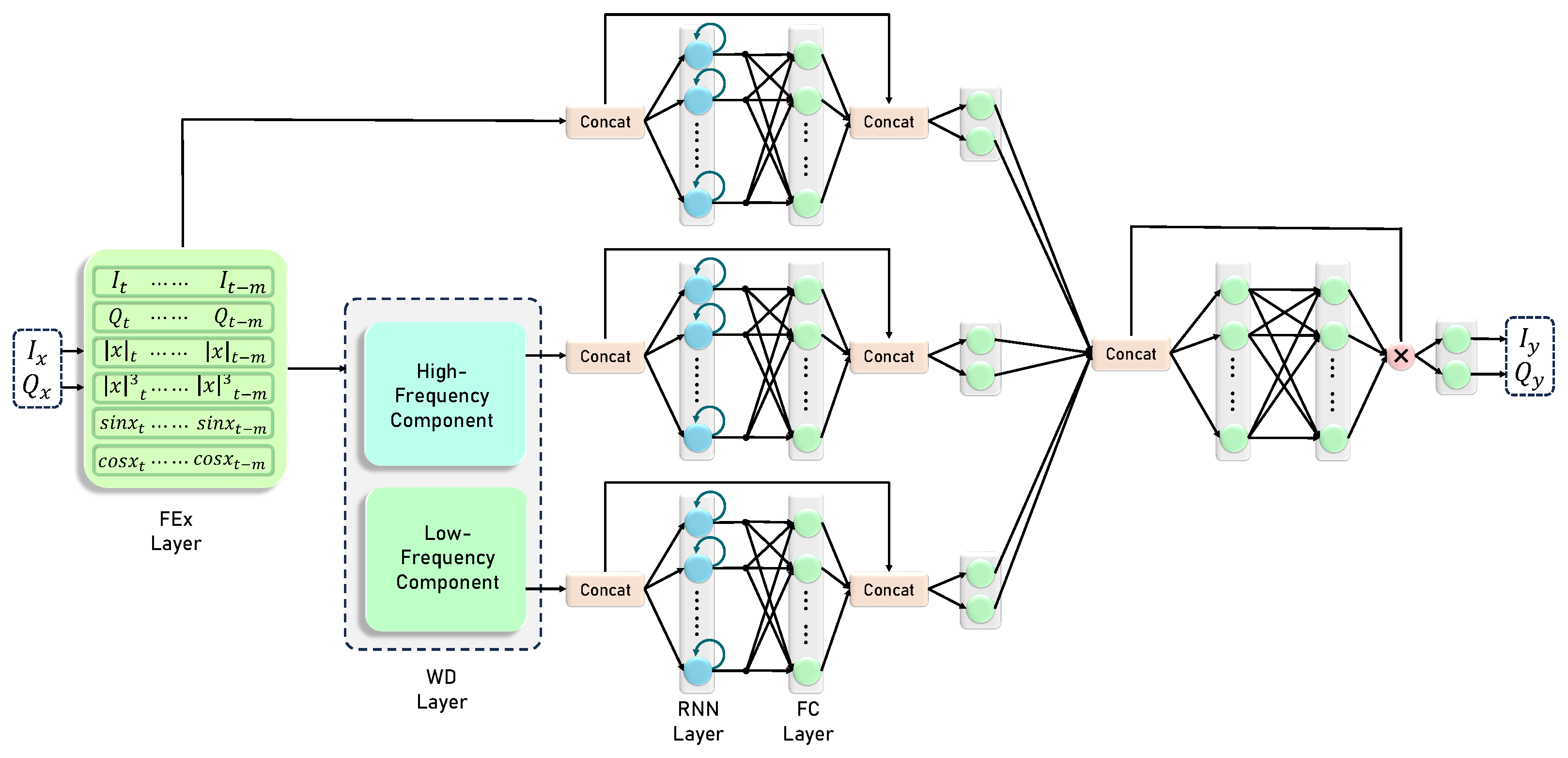
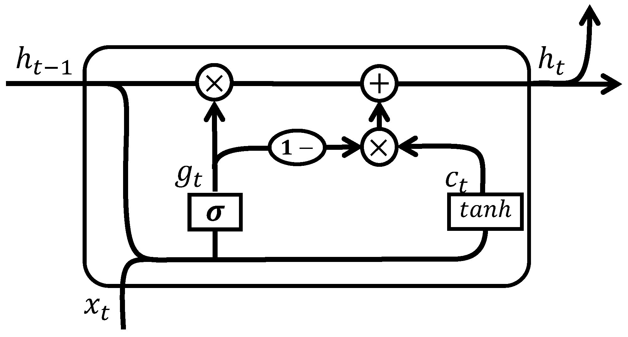
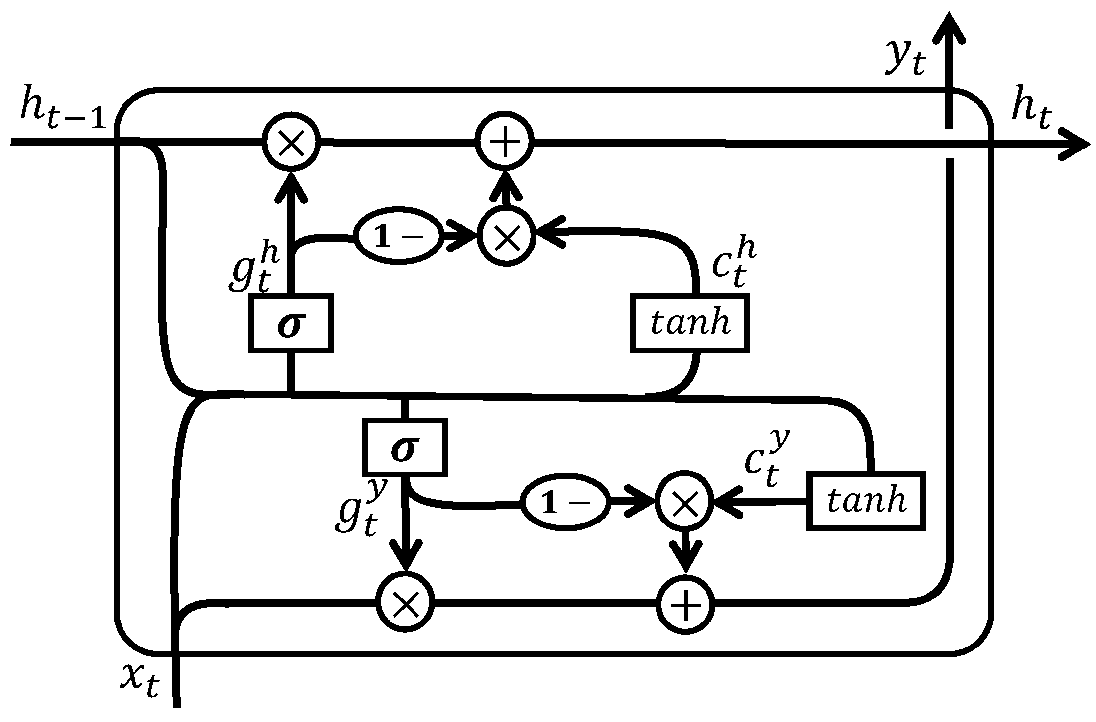
  • Our approach integrates a dual-stage RNN composed of a UGRNN and an IRNN, both of which extend the vanilla RNN with a lightweight gating mechanism. Specifically, the UGRNN is employed for PA nonlinear modeling, while the IRNN is used in the DPD stage, ensuring that each stage leverages the most suitable RNN variant.
  • We develop a learnable WD module that leverages WD’s frequency learning capability to decompose signals into higher-frequency components, facilitating more effective analysis of distorted signals.
  • We perform extensive simulations on the open-source dataset “OpenDPD”, demonstrating substantial improvements over state-of-the-art WDP-based methods, including a 4.59 dB reduction in the NMSE, ACPR gains of 3.37 / 4.82 dBc, and a 5.14 dB improvement in the EVM.

2. System Model and Problem Description

2.1. System Model

WDP initially captures the input and output signals of the PA and employs a neural network to accurately model its nonlinear behavior. In this stage, the model’s output remains nonlinear. Once the PA nonlinear model is trained, its parameters are frozen, and it is cascaded with the DPD model. By training this cascaded system to linearize its output, the DPD model is indirectly optimized.

2.2. Problem Formulation

WDP encompasses both PA nonlinear modeling and DPD modeling, so we decompose the problem into two parts for a clearer explanation.
In the following formulation, D tr denotes the training set, and N represents the sample length. The PA input and output signals are denoted by x and y , respectively, both of which include I/Q components represented as I x , Q x , I y , and Q y . The sample spaces of the PA input and output signals are X and Y . The function f Mod ( · ) represents the output of the PA nonlinear model, while f DPD ( · ) corresponds to the output function of the DPD model. The PA’s output function is denoted as f PA ( · ) . The expectation operator is represented by E , and L MSE refers to the mean squared error (MSE) loss function. The nonlinear output of the PA model is denoted by y ^ , which is computed as
y ^ = f Mod ( x ) .
After applying DPD, the cascaded model produces a linear output, represented as y ¯ , which is given by
y ¯ = f PA ( f DPD ( x ) ) .
Finally, A denotes the gain of the PA, which is computed as
A = 1 N n = 0 N 1 I y 2 [ n ] + Q y 2 [ n ] I x 2 [ n ] + Q x 2 [ n ] .
The dataset for WDP includes the input and output signals of the PA in each time step as
D t r = x n , y n n = 0 N 1 .
The problem with PA nonlinear modeling is to generate a mapping function, f Mod F : X Y , and ensure the ability to simulate the nonlinearity of the PA. The expected nonlinear model output error is minimized as
min f Mod F E y , y ^ L MSE y , y ^ .
The goal of the DPD problem is to generate a mapping function, f DPD G : A · X Y , and ensure that the output of the PA is linear. Its expected model output error is minimized as
min f DPD G E A · x , y ¯ L MSE A · x , y ¯ .
.

3. The Proposed WDP Architecture

To achieve a more accurate predistortion model, we adopt an WDP-based approach. The detailed workflow is illustrated in Figure 1.
The first stage involves PA nonlinear modeling, where the input and output signals of the PA are used to train a nonlinear model through a neural network. Initially, a feature extraction (FEx) layer is employed to derive additional features from the I/Q signal, computing x , x 3 , sin x , and cos x [27]. Subsequently, WD is utilized to decompose these features into different frequency components, enabling more effective multi-resolution analysis [28]. To capture long-term dependencies in the data, the UGRNN is employed. After the UGRNN processes and analyzes various frequency components [29], a self-attention mechanism is incorporated to balance their impact on the output. The overall framework of WDP is depicted in Figure 2, where the RNN module can be implemented using either the UGRNN or IRNN [30].
The second stage focuses on DPD modeling. The DPD model is cascaded with the PA nonlinear model, where the output of the DPD model serves as the input to the PA nonlinear model. The parameters of the PA nonlinear model in this cascaded system are directly copied and frozen from the model trained in the first stage. WD is again applied for feature processing in this step. The IRNN is then utilized to capture long-term dependencies, and a self-attention mechanism, as in the first stage, is employed to refine the output. The entire procedure is outlined in Algorithm 1.
Algorithm 1 The detailed procedures of the proposed WDP method.
Require:
  • D t r , D t e : Training dataset, test dataset;
  • T: Number of training iterations;
  • B: Number of batches in a training iteration;
  • Z: Length of the short frame;
  • V: Stride of the short frame;
  • θ Mod , θ DPD : Parameters of PA and DPD model;
  • l r : Learning rate of optimizer;
  • m: Memory depth;
Preparation:
  • Get ( x , y ) from D t r .
  • Calculate the A by Equation (3).
  • Split features and labels into a shorter frame, each of size Z, with a stride of V. Consecutive frames overlap by Z V samples.
  • Extract features and calculate I , Q , x , x 3 , sin x and cos x .
  • Processing feature vectors based on m, denoted as S .
  • Perform a one-level WD on S , and the high and low frequency components are denoted as S l and S h .
Applsci 15 03599 i001
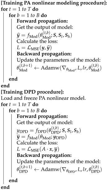
[Testing procedure]:
  • Get ( x , y ) from D t r .
  • Get S , S l , S h through preparation.
  • Obtain DPD output: y DPD = f DPD ( θ DPD ; S , S l , S h ) .

3.1. PA Nonlinear Modeling by WDP

During the PA nonlinear modeling stage, we adopt a combination of WD and UGRNN methods, where WD serves as a signal analysis technique that extracts time-frequency features by progressively decomposing the time series into low-frequency and high-frequency subsequences.
We define the input time series as x = x 1 , , x m , , x M . The high-frequency and low-frequency subsequences generated at the i-th decomposition layer are denoted as x h ( i ) and x l ( i ) , respectively. At the ( i + 1 ) -th level, WD applies a low-pass filter, l = l 1 , , l k , , l K , and a high-pass filter, h = h 1 , , h k , , h K , where K M . The low-frequency components from the previous layer are then convolved as
a n l i + 1 = k = 1 K x n + k 1 l i · l k ,
a n h i + 1 = k = 1 K x n + k 1 l i · h k ,
where x n l ( i ) represents the n-th element of the low-frequency component at the i-th decomposition layer. The low-frequency x l ( i ) and high-frequency x h ( i ) components at the i-th layer are derived from the 1 2 down-sampling of the intermediate variable sequences a l ( i ) = a 1 l ( i ) , a 2 l ( i ) , and a h ( i ) = a 1 h ( i ) , a 2 h ( i ) , .
The method proposed in [29] can approximate the implementation of WD within a NN architecture. The WD model decomposes time series using the following two functions:
a l i = W l i x l i 1 + b l i ,
a h i = W h i x h i 1 + b h i ,
where b l i and b h i are trainable bias vectors, and their initial values are all random values close to zero. It is not difficult to find that Equations (7)–(10) have the same form of WD function. x n l i and x n h i are the n-th elements of the low-frequency and high-frequency components in the i-th layer, respectively, which are down-sampled from the intermediate variables a l i and a h i using average pooling.
To achieve the convolution defined in Equation (3), it is necessary to set the initial values of the weight matrices W l i and W h i as
W l i = l 1 l 2 l 3 l K ε ε ε l 1 l 2 l K 1 l K ε ε ε ε l 1 l K 1 l K ε ε ε l 1 l 2 ε ε ε ε l 1 ,
W h i = h 1 h 2 h 3 h K ε ε ε h 1 h 2 h K 1 h K ε ε ε ε h 1 h K 1 h K ε ε ε h 1 h 2 ε ε ε ε h 1 ,
where W l i and W h i R P × P , and P is the size of x l i 1 . The values in the weight matrix that do not belong to the filter coefficients are filled with a random value, ε , where the random value ε needs to satisfy ε l , l l , and ε h , h h . Setting ε to a very small value is because, even though these parameters are not part of the core of the filter, setting them to a very small value can still preserve the trainability of the network to some extent. This is particularly helpful in the early stages of training, as it allows the network to converge to a more optimal solution. In this paper, we chose the Daubechies 4 (Db4) wavelet because it offers a good balance between compact support, smoothness, and orthogonality, making it particularly effective for signal processing tasks. More importantly, the characteristics of Db4 align well with the demands of DPD tasks, where capturing both sharp transitions and subtle signal variations is crucial for accurate nonlinear compensation. In detail, the filter coefficients were set as
l = { 0.0106 , 0.0329 , 0.0308 , 0.187 , 0.028 , 0.6309 , 0.7148 , 0.2304 } ,
h = { 0.2304 , 0.7148 , 0.6309 , 0.028 , 0.187 , 0.0308 , 0.0329 , 0.0106 } ,
It was observed that the gating mechanism was pivotal in the selection of the RNN. After evaluating various configurations, we opted to integrate a vanilla RNN with a straightforward gating mechanism. Through extensive experimentation, the UGRNN was selected as the preferred RNN architecture for modeling the nonlinearity of the PA [30]. The gating mechanism in a UGRNN serves to regulate whether the hidden state is retained from the previous time step or updated with new information. The internal structure of a UGRNN network unit is illustrated in Figure 3, and the transition functions of a UGRNN are defined as follows:
c t = tanh W c h h t 1 + W c x x t + b c ,
g t = σ W g h h t 1 + W g x x t + b g ,
h t = g t · h t 1 + 1 g t · c t ,
In this formulation, c t represents the unit state, which is influenced by both the hidden state from the previous unit, h t 1 , and the current input, x t . The tanh activation determines how information is stored in the current unit. The gating mechanism, represented by g t , regulates the flow of information by leveraging the sigmoid function to balance contributions from the previous hidden state and the current input. Equation (17) updates the unit’s hidden state by merging the functions of the forget and input gates into a unified update gate. Notably, the role of g t must be considered, as 1 g t represents the forgotten information. Ultimately, the hidden state of the RNN serves as the model’s output.
The extracted features, along with the high-frequency and low-frequency components obtained via WD processing, are fed into the UGRNN. Distorted signals often contain a mixture of frequency components, particularly in the high-frequency range. By applying WD, the signal is decomposed into high- and low-frequency components, enabling the model to process them separately and capture distortion features more effectively. Meanwhile, features that bypass WD retain global information, providing a broader context for the model. To enhance the model’s ability to utilize different frequency characteristics, we incorporate a self-attention mechanism that evaluates the impact of high-frequency, low-frequency, and raw components on the output. By dynamically assigning weights based on input characteristics, the self-attention mechanism determines the relative importance of each component. This adaptability allows it to adjust the contributions of different frequency components depending on the input signal, thereby improving the model’s robustness and generalization across varying signal conditions.

3.2. DPD by WDP

During the DPD modeling stage, we adopt a combination of WD and IRNN methods, where WD serves the same function as in PA nonlinear modeling. For the recurrent network, we utilize an IRNN. Similarly to the UGRNN, the IRNN combines a vanilla RNN with a simple gating mechanism. However, the IRNN differs in that it employs separate gating mechanisms for the hidden state and output. The internal structure of the IRNN unit is illustrated in Figure 4. The transition functions of the IRNN are defined as follows:
c 1 t = tanh W c 1 h h t 1 + W c 1 x x t + b c 1 ,
c 2 t = tanh W c 2 h h t 1 + W c 2 x x t + b c 2 ,
g 1 t = σ W g 1 h h t 1 + W g 1 x x t + b g 1 ,
g 2 t = σ W g 2 h h t 1 + W g 2 x x t + b g 2 ,
y t = g 1 t · x t + 1 g 1 t · c 1 t ,
h t = g 2 t · x t + 1 g 2 t · c 2 t ,
The functions of c 1 t , c 2 t , and c t are identical, just as g 1 t and g 2 t share the same role as g t . Unlike that of the UGRNN, the output of the IRNN is not the hidden state but a redefined output, as described in Equation (22). Although the IRNN introduces more parameters compared to the UGRNN, it provides better control over the model’s output.

4. Experimental Results and Discussions

4.1. Experimental Setup

The details of our experimental setup are presented in Table 1. The dataset, provided by [27], consists of 38,400 samples of 200 MHz orthogonal frequency division multiplexing (OFDM) signals, sampled at an 800 MHz rate. The I/Q data were processed using a 40 nm CMOS-based digital transmitter and digitized by an R&S-FSW8 analyzer. The dataset was split into a training set (60%), validation set (20%), and testing set (20%). Moreover, we strictly followed the standard procedures outlined by the OpenDPD dataset for experimentation and validation, using its provided training and testing datasets to ensure consistency with established evaluation methodologies.
In addition, we used AdamW as the optimizer with the ReduceLROnPlateau scheduler and ensured training stability by carefully adjusting optimization settings, including tuning the learning rate, selecting appropriate activation functions, and monitoring gradient variations to prevent instability or overfitting.
The experiment evaluated the quality of the model by calculating the NMSE, the simulated (SIM)-ACPR, and the SIM-EVM as
NMSE = n = 0 N 1 I y ¯ n I y ˜ n 2 + Q y ¯ n Q y ˜ n 2 n = 0 N 1 I y ˜ 2 n + Q y ˜ 2 n ,
ACPR = P adj P main ,
EVM = k = 0 K 1 I y ¯ k I y ˜ k 2 + Q y ¯ k Q y ˜ k 2 k = 0 K 1 I y ˜ 2 k + Q y ˜ 2 k ,
where y ¯ and y ˜ are cascaded models and desired outputs, respectively. P main and P adj are the main and adjacent channel powers, respectively. I k and Q k are in-phase and quadrature signal components after an FFT. The SIM-ACPR and SIM-EVM were calculated through software. It is confirmed in [27] that the SIM-ACPR and SIM-EVM have reliable consistency with the ACPR and EVM.

4.2. Analysis of PA Nonlinear Modeling

To evaluate the variability introduced by random initialization during training, we conducted five independent training and testing runs for each model using different random seeds. The results are presented as the average metric values along with their standard deviations. The effectiveness of our proposed approach for PA nonlinear modeling was assessed against several established methods, including vector decomposition LSTM (VDLSTM) [31], the real-valued time-delayed convolutional neural network (RVTDCNN) [32], the dense gated recurrent unit (DGRU), the Feature+GRU [27], and the UGRNN [30]. VDLSTM incorporates phase information recovery during linearization [33,34], the RVTDCNN is a well-known CNN-based model for DPD tasks [13], while the DGRU and Feature+GRU represent state-of-the-art techniques for WDP-based DPD. The hyperparameters for the comparative models were aligned with those specified in [27].
As shown in Table 2, WDP achieved the lowest error and the highest modeling accuracy, with an NMSE of 34.96 dB. Consequently, WDP was selected for the nonlinear modeling of the PA. Since the PA output was influenced by both nonlinearity and memory effects, it was essential to account for both factors in the modeling process. The WDP approach, leveraging the FEx layer, computed x , x 3 , sin x , and cos x from the I/Q values. Here, x and x 3 represent envelope-related terms that capture the PA’s nonlinear characteristics, while sin x and cos x incorporate the PA’s phase information, which further reflects its nonlinear behavior. In WDP, WD separated the signal into high-frequency and low-frequency components, allowing the model to effectively analyze the nonlinearity embedded in the signal. Additionally, WD incorporated memory terms during the signal decomposition process, enabling the UGRNN to better capture long-term dependencies within the signal. Since PA distortion arises from the combined influence of nonlinearity and memory effects, the WDP modeling process closely aligned with the physical nature of PA nonlinear distortion. This alignment explains why WDP demonstrated such high accuracy in PA nonlinear modeling. From Table 2, it is evident that the UGRNN alone did not achieve the same level of accuracy as WDP, underscoring the effectiveness of the WD module in enhancing modeling performance.

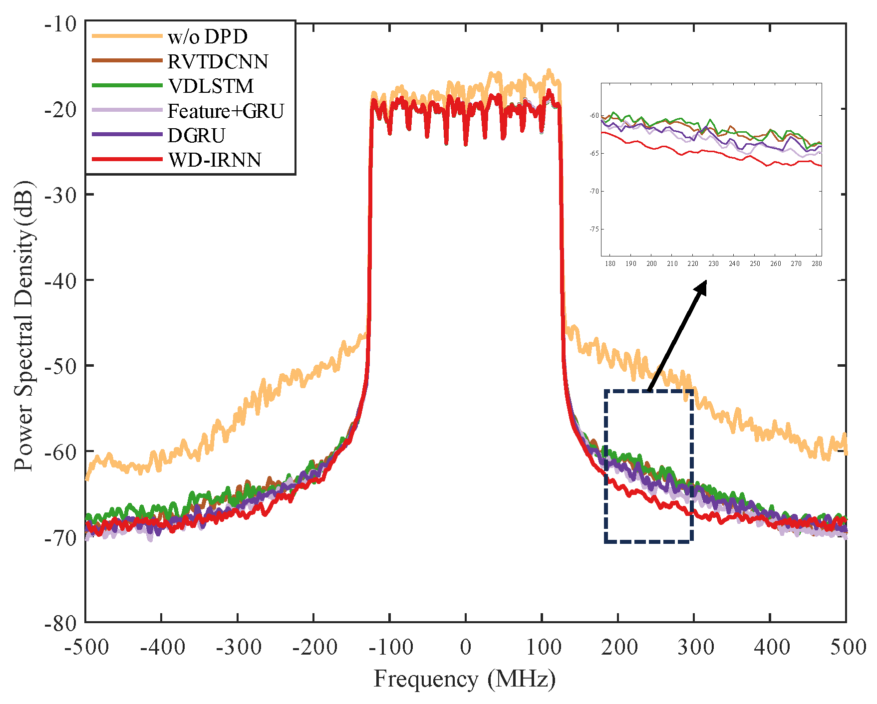
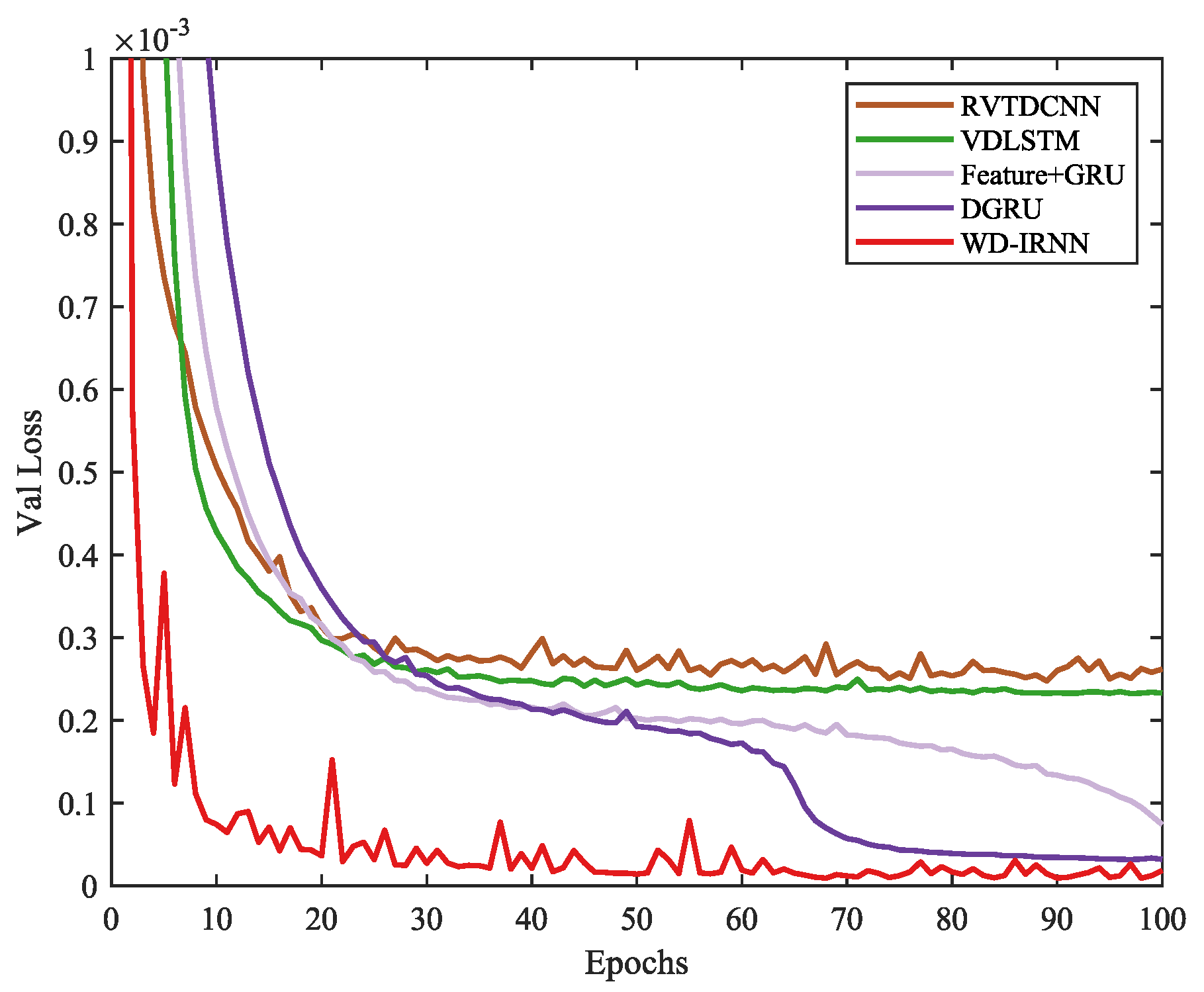
4.3. Analysis of DPD Modeling

For DPD experiments, we leveraged the WDP model due to its superior modeling accuracy. The DPD performance was evaluated by training the model with five different random seeds and comparing it against VDLSTM, the RVTDCNN, the DGRU, the Feature+GRU, the IRNN, and WDP. The results, presented in Table 3, demonstrate that WDP outperformed all other methods across three key metrics: it achieved an NMSE of 45.51 dB, an ACPR of 52.71 / 51.93 dB, and an EVM of 48.92 dB. Compared to the latest state-of-the-art methods, WDP showed improvements of 4.59 dB in the NMSE, 3.37 / 4.82 dB in the ACPR, and 5.14 dB in the EVM. Furthermore, WDP significantly outperformed traditional DPD methods. When compared to VDLSTM, the DGRU, and the Feature+GRU, WDP demonstrated the best performance among RNN-based architectures. Additionally, RNN-based methods like WDP were shown to be more effective than CNN-based approaches such as the RVTDCNN in addressing PA nonlinearity. Among the compared models, the DGRU, the Feature+GRU, the IRNN, and WDP all utilized I/Q, x , x 3 , sin x , and cos x features, highlighting WDP’s superior feature extraction capability and its effectiveness in handling PA nonlinearity. The performance gap between WDP and the IRNN further underscores the significant contribution of the WD module in enhancing the overall DPD performance.

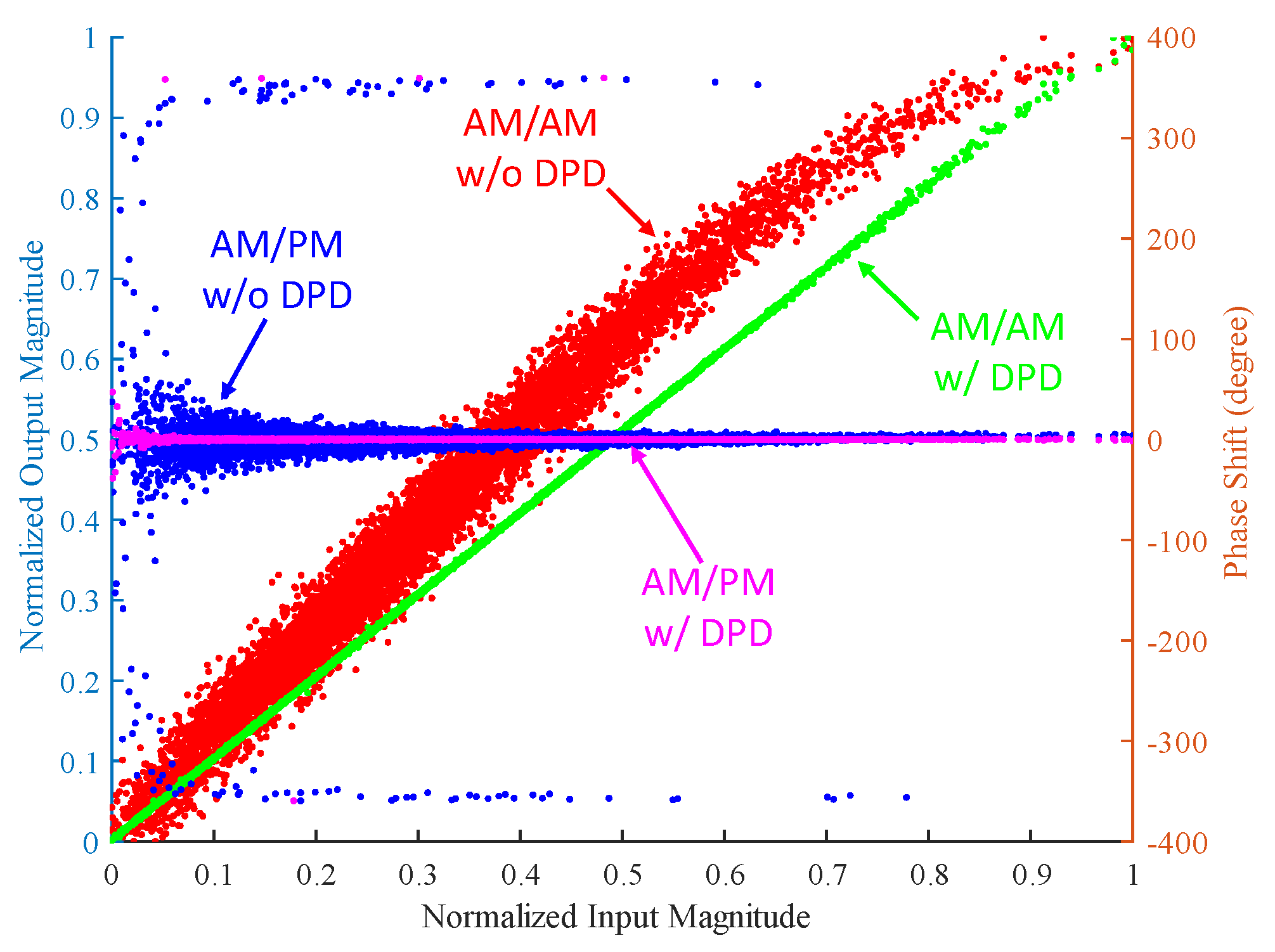
4.4. Visual Interpretation

PA nonlinear distortion can impact adjacent channels. To test this, we used a 200 MHz OFDM signal, which makes linearization more difficult. As illustrated in Figure 5, the signal without DPD processing significantly affected adjacent channels; however, after DPD processing, this issue was substantially improved. Among the methods tested, WDP showed the greatest improvement in the spectrum. Despite the high degree of PA nonlinear distortion, the results shown in Figure 6 for amplitude modulation (AM) and AM-phase modulation (PM) with and without DPD demonstrate that WDP excelled at linearizing distorted signals in the 200 MHz OFDM signal, effectively mitigating PA nonlinearity and significantly reducing memory effects. Furthermore, Figure 7 presents the loss curves of various models on the validation set. It is evident that WDP not only converged the fastest but also achieved the lowest loss value, whereas other DPD methods showed slower convergence and higher loss values throughout the training process. All methods were trained on the same dataset, ensuring a fair comparison. The results highlight that the integration of wavelet decomposition and RNNs enabled WDP to more effectively capture the nonlinear features of signals, contributing to its superior fitting performance.

5. Conclusions

In this paper, we employed the WDP approach for nonlinear PA and DPD modeling. Unlike direct and indirect learning methods, this approach enabled the direct training of the DPD model, offering the advantage of directly calculating the predistortion coefficient, leading to more accurate parameter estimation. We applied WD to DPD tasks for the first time and demonstrated its effectiveness. The performance of the WDP was validated through experimental testing, achieving an NMSE of 45.51 dB, an ACPR of −52.71/−51.93 dBc, and an EVM of 48.92 dB. The results indicate that WDP effectively handled the PA’s nonlinear distortion and phase shift, delivering excellent linearization performance. In future work, we plan to evaluate our method under high-noise and -distortion conditions in real RF environments, seeking collaborative opportunities and necessary experimental equipment for further validation. Additionally, we aim to systematically analyze the impact of different hyperparameter settings and minimum sample size requirements to enhance the generalizability and robustness of our approach.

Author Contributions

Methodology, S.P.; validation, S.P.; formal analysis, S.P.; investigation, S.P.; resources, J.Y.; writing—original draft preparation, S.P.; writing—review and editing, S.P.; visualization, S.P.; supervision, J.Y.; funding acquisition, J.Y. All authors have read and agreed to the published version of the manuscript.

Funding

This research was funded by the Science and Technology Project of Jiangsu Provincial Administration for Market Regulation in 2023 grant number KJ2023053.

Institutional Review Board Statement

Not applicable.

Informed Consent Statement

Not applicable.

Data Availability Statement

The original contributions presented in the study are included in the article, further inquiries can be directed to the corresponding author.

Conflicts of Interest

The authors declare no conflicts of interest.

References

  1. Zhang, Q.; Jiang, C.; Yang, G.; Han, R.; Liu, F. Multi-Output Recurrent Neural Network Behavioral Model for Digital Predistortion of RF Power Amplifiers. IEEE Microw. Wirel. Technol. Lett. 2023, 33, 1067–1070. [Google Scholar] [CrossRef]
  2. Aguila-Torres, D.S.; Galaviz-Aguilar, J.A.; Cárdenas-Valdez, J.R. Reliable Comparison for Power Amplifiers Nonlinear Behavioral Modeling Based on Regression Trees and Random Forest. In Proceedings of the 2022 IEEE International Symposium on Circuits and Systems (ISCAS), Austin, TX, USA, 27 May–1 June 2022. [Google Scholar]
  3. He, Z.; Tong, F. Residual RNN Models with Pruning for Digital Predistortion of RF Power Amplifiers. IEEE Trans. Veh. Technol. 2022, 71, 9735–9750. [Google Scholar] [CrossRef]
  4. Omar, M.S.; Qi, J.; Ma, X. Mitigating Clipping Distortion in Multicarrier Transmissions Using Tensor-Train Deep Neural Networks. IEEE Trans. Wirel. Commun. 2023, 22, 2127–2138. [Google Scholar] [CrossRef]
  5. Lopez-Bueno, D.; Wang, T.; Gilabert, P.L.; Montoro, G. Amping Up, Saving Power: Digital Predistortion Linearization Strategies for Power Amplifiers under Wideband 4G/5G Burst-Like Waveform Operation. IEEE Microw. Mag. 2015, 17, 79–87. [Google Scholar] [CrossRef]
  6. He, Z. Time-Delay/Advance Neural Networks Based Digital Predistorters: Enabling High Efficiency and High Throughput Transmitter. In Proceedings of the 2023 IEEE Wireless Communications and Networking Conference (WCNC), Glasgow, UK, 26–29 March 2023. [Google Scholar]
  7. Younes, M. An Accurate Complexity-Reduced “PLUME” Model for Behavioral Modeling and Digital Predistortion of RF Power Amplifiers. IEEE Trans. Ind. Electron. 2011, 58, 1397–1405. [Google Scholar] [CrossRef]
  8. Chen, W.; Liu, X.; Chu, J.; Wu, H.; Feng, Z.; Ghannouchi, F.M. A Low Complexity Moving Average Nested GMP Model for Digital Predistortion of Broadband Power Amplifiers. IEEE Trans. Circuits Syst. I Regul. Pap. 2022, 69, 2070–2083. [Google Scholar] [CrossRef]
  9. Zhu, A. Decomposed Vector Rotation-Based Behavioral Modeling for Digital Predistortion of RF Power Amplifiers. IEEE Trans. Microw. Theory Tech. 2015, 63, 737–744. [Google Scholar] [CrossRef]
  10. Wang, D.; Aziz, M.; Helaoui, M.; Ghannouchi, F.M. Augmented Real-Valued Time-Delay Neural Network for Compensation of Distortions and Impairments in Wireless Transmitters. IEEE Trans. Neural Netw. Learn. Syst. 2019, 30, 242–254. [Google Scholar] [CrossRef]
  11. Zhang, Y.; Li, Y.; Liu, F.; Zhu, A. Vector Decomposition Based Time-Delay Neural Network Behavioral Model for Digital Predistortion of RF Power Amplifiers. IEEE Access 2019, 7, 91559–91568. [Google Scholar] [CrossRef]
  12. Kobal, T.; Li, Y.; Wang, X.; Zhu, A. Digital Predistortion of RF Power Amplifiers with Phase-Gated Recurrent Neural Networks. IEEE Trans. Microw. Theory Tech. 2022, 70, 3291–3299. [Google Scholar] [CrossRef]
  13. Jiang, C.; Li, H.; Qiao, W.; Yang, G.; Liu, Q.; Wang, G.; Liu, F. Block-Oriented Time-Delay Neural Network Behavioral Model for Digital Predistortion of RF Power Amplifiers. IEEE Trans. Microw. Theory Tech. 2022, 70, 1461–1473. [Google Scholar] [CrossRef]
  14. Wu, Y.; Li, A.; Beikmirza, M.; Singh, G.D.; Chen, Q.; de Vreede, L.C.N.; Alavi, M.; Gao, C. MP-DPD: Low-Complexity Mixed-Precision Neural Networks for Energy-Efficient Digital Predistortion of Wideband Power Amplifiers. IEEE Microw. Wirel. Technol. Lett. 2024, 34, 817–820. [Google Scholar]
  15. Paaso, H.; Mammela, A. Comparison of Direct Learning and Indirect Learning Predistortion Architectures. In Proceedings of the 2008 IEEE International Symposium on Wireless Communication Systems, Reykjavik, Iceland, 21–24 October 2008. [Google Scholar]
  16. Landin, P.N.; Mayer, A.E.; Eriksson, T. MILA—A Noise Mitigation Technique for RF Power Amplifier Linearization. In Proceedings of the 2014 IEEE 11th International Multi-Conference on Systems, Signals & Devices (SSD14), Barcelona, Spain, 11–14 February 2014. [Google Scholar]
  17. Abi Hussein, M.; Bohara, V.A.; Venard, O. On the System Level Convergence of ILA and DLA for Digital Predistortion. In Proceedings of the 2012 International Symposium on Wireless Communication Systems (ISWCS), Paris, France, 28–31 August 2012. [Google Scholar]
  18. Mengozzi, M.; Gibiino, G.P.; Angelotti, A.M.; Florian, C.; Santarelli, A. GaN power amplifier digital predistortion by multi-objective optimization for maximum RF output power. Electronics 2021, 10, 244. [Google Scholar] [CrossRef]
  19. Wang, X.; Li, Y.; Yin, H.; Yu, C.; Yu, Z.; Hong, W.; Zhu, A. Digital Predistortion of 5G Multiuser MIMO Transmitters Using Low-Dimensional Feature-Based Model Generation. IEEE Trans. Microw. Theory Tech. 2021, 70, 1509–1520. [Google Scholar] [CrossRef]
  20. Mengozzi, M.; Gibiino, G.P.; Angelotti, A.M.; Florian, C.; Santarelli, A. Beam-dependent active array linearization by global feature-based machine learning. IEEE Microw. Wirel. Compon. Lett. 2023, 33, 895–898. [Google Scholar] [CrossRef]
  21. Zhou, D.; DeBrunner, V.E. Novel Adaptive Nonlinear Predistorters Based on The Direct Learning Algorithm. IEEE Trans. Signal Process. 2007, 55, 120–133. [Google Scholar]
  22. Yu, Z.; Zhu, E. A Comparative Study of Learning Architecture for Digital Predistortion. In Proceedings of the 2015 Asia-Pacific Microwave Conference (APMC), Nanjing, China, 6–9 December 2015. [Google Scholar]
  23. Wang, Z.; Chen, W.; Su, G.; Ghannouchi, F.M.; Feng, Z.; Liu, Y. Low Computational Complexity Digital Predistortion Based on Direct Learning With Covariance Matrix. IEEE Trans. Microw. Theory Tech. 2017, 65, 4274–4284. [Google Scholar]
  24. Tarver, C.; Jiang, L.; Sefidi, A.; Cavallaro, J.R. Neural network DPD via backpropagation through a neural network model of the PA. In Proceedings of the 2019 53rd Asilomar Conference on Signals, Systems, and Computers, Pacific Grove, CA, USA, 3–6 November 2019. [Google Scholar]
  25. Javid-Hosseini, S.H.; Ghazanfarianpoor, P.; Nayyeri, V.; Colantonio, P. A Unified Neural Network-Based Approach to Nonlinear Modeling and Digital Predistortion of RF Power Amplifier. IEEE Trans. Microw. Theory Tech. 2024, 72, 5031–5038. [Google Scholar]
  26. Ghazanfarianpoor, P.; Javid-Hosseini, S.H.; Abbasnezhad, F.; Arian, A.; Nayyeri, V.; Colantonio, P. A Neural Network-Based Pre-Distorter for Linearization of RF Power Amplifiers. In Proceedings of the 2023 22nd Mediterranean Microwave Symposium (MMS), Sousse, Tunisia, 30 October–1 November 2023. [Google Scholar]
  27. Wu, Y.; Singh, G.D.; Beikmirza, M.; de Vreede, L.C.N.; Alavi, M.; Gao, C. OpenDPD: An Open-Source End-to-End Learning & Benchmarking Framework for Wideband Power Amplifier Modeling and Digital Pre-Distortion. In Proceedings of the 2024 IEEE International Symposium on Circuits and Systems (ISCAS), Singapore, 19–22 May 2024. [Google Scholar]
  28. Wan, R.; Mei, S.; Wang, J.; Liu, M.; Yang, F. Multivariate Temporal Convolutional Network: A Deep Neural Networks Approach for Multivariate Time Series Forecasting. Electronics 2019, 8, 876. [Google Scholar] [CrossRef]
  29. Wang, J.; Wang, Z.; Li, J.; Wu, J. Multilevel Wavelet Decomposition Network for Interpretable Time Series Analysis. In Proceedings of the 24th ACM SIGKDD International Conference on Knowledge Discovery & Data Mining, London, UK, 19–23 August 2018. [Google Scholar]
  30. Collins, J.; Sohl-Dickstein, J.; Sussillo, D. Capacity and Trainability in Recurrent Neural Networks. Available online: https://arxiv.org/abs/1611.09913 (accessed on 29 November 2016).
  31. Li, H.; Zhang, Y.; Li, G.; Liu, F. Vector Decomposed Long Short-Term Memory Model for Behavioral Modeling and Digital Predistortion for Wideband RF Power Amplifiers. IEEE Access 2020, 8, 63780–63789. [Google Scholar]
  32. Hu, X.; Liu, Z.; Yu, X.; Zhao, Y.; Chen, W.; Hu, B.; Du, X.; Li, X.; Helaoui, M.; Wang, W.; et al. Convolutional Neural Network for Behavioral Modeling and Predistortion of Wideband Power Amplifiers. IEEE Trans. Neural Netw. Learn. Syst. 2022, 33, 3923–3937. [Google Scholar] [PubMed]
  33. Zhang, Q.; Jiang, C.; Yang, G.; Han, R.; Liu, F. Block-Oriented Recurrent Neural Network for Digital Predistortion of RF Power Amplifiers. IEEE Trans. Microw. Theory Tech. 2024, 72, 3875–3885. [Google Scholar]
  34. Chani-Cahuana, J.; Landin, P.N.; Fager, C.; Eriksson, T. Iterative Learning Control for RF Power Amplifier Linearization. IEEE Trans. Microw. Theory Tech. 2016, 64, 2779–2789. [Google Scholar]
Figure 1. Detailed steps for the proposed WDP architeture.
Applsci 15 03599 g001
Figure 2. The framework of WDP, where the RNN is replaced with the UGRNN in the PA modeling phase and with the IRNN in the DPD phase.
Applsci 15 03599 g002
Figure 3. Internal structure of UGRNN unit.
Applsci 15 03599 g003
Figure 4. Internal structure of IRNN network unit.
Applsci 15 03599 g004
Figure 5. Linearization performance of PA using various methods.
Applsci 15 03599 g005
Figure 6. PA characteristics with and without WDP.
Applsci 15 03599 g006
Figure 7. Validation loss comparison of different DPD methods over training epochs.
Applsci 15 03599 g007
Table 1. Relevant information about experiments.
ItemsSetting
Python3.9.19
Pytorch1.12.0
Training epochs100
Batch size64
Memory depth24
Frame length50
Optimizer for modelAdamw (learning rate = 0.001)
PlatformNVIDIA GeForce GTX 2080Ti GPU
Table 2. PA nonlinear modeling performance comparison of various methods.
Modeling MethodsNMSE (dB)
RVTDCNN [32] 28.48 ± 0.04
VDLSTM [31] 28.57 ± 0.02
Feature+GRU [27] 31.50 ± 0.20
DGRU [27] 31.54 ± 0.11
UGRNN [30] 31.32 ± 0.15
WDP (Ours) 34.96 ± 0.08
Table 3. DPD performance comparison of various methods.
DPD MethodsNMSE (dB)SIM-ACPR (dBc, L/R)SIM-EVM (dB)
RVTDCNN [32] 31.26 ± 0.15 −44.49 ± 0.95/−44.10 ± 0.83 33.88 ± 0.14
VDLSTM [31] 31.73 ± 0.11 −45.92 ± 0.23/−45.37 ± 0.79 34.44 ± 0.15
Feature+GRU [27]−40.92 ± 3.96−49.34 ± 0.52/−47.11 ± 0.82 43.78 ± 3.92
DGRU [27] 39.62 ± 3.55 −49.14 ± 0.64/−46.06 ± 0.89 42.43 ± 3.54
IRNN [30] 34.76 ± 1.81 −47.85 ± 1.12/−46.81 ± 0.99 35.84 ± 1.97
WDP (Ours) 45.51 ± 0.65 52.71 ± 0.78/51.93 ± 0.61 48.92 ± 0.83
Disclaimer/Publisher’s Note: The statements, opinions and data contained in all publications are solely those of the individual author(s) and contributor(s) and not of MDPI and/or the editor(s). MDPI and/or the editor(s) disclaim responsibility for any injury to people or property resulting from any ideas, methods, instructions or products referred to in the content.

