Enhanced MCDM Based on the TOPSIS Technique and Aggregation Operators Under the Bipolar pqr-Spherical Fuzzy Environment: An Application in Firm Supplier Selection

 , , ,
, , ,
Abstract
1. Introduction
Extensions of Fuzzy Set Theory: Review
2. Background Concepts
- 1.
- 2.
- 3.
- 4.
- 1.
- 2.
- 3.
- 4.
- 1.
- 2.
- 3.
- 4.
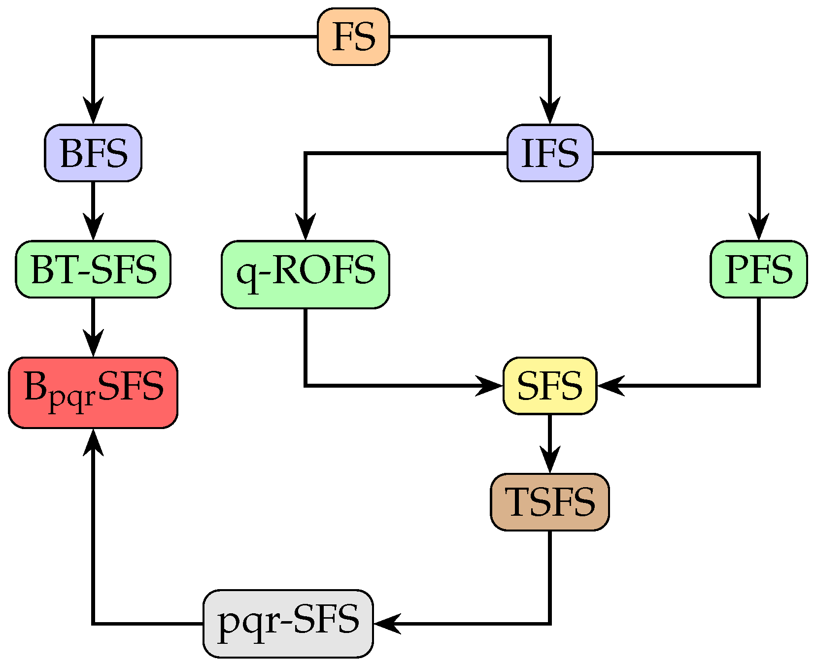
3. Bipolar pqr-Spherical Fuzzy Sets
- 1.
- bipolar T-spherical fuzzy set (BT-SFS) [23] if .
- 2.
- spherical bipolar fuzzy set (SBFS) [22] if .
- 3.
- bipolar picture fuzzy set (BPFS) [24] if .
- 4.
- bipolar mn-rung orthopair fuzzy set (Bmn-ROFS) [21] if .
- 5.
- Fermatean bipolar fuzzy set (FBFS) [19] if and .
- 6.
- bipolar Pythagorean fuzzy set (BPyFS) [18] if and .
- 7.
- bipolar intuitionistic fuzzy set (BIFS) [17] if and .
- 8.
- 9.
- T-spherical fuzzy set (T-SFS) [9] if and .
- 10.
- 11.
- picture fuzzy set (PFS) [8] if and .
- 12.
- p,q-quasirung orthopair fuzzy set (pq-QROFS) [6] if .
- 13.
- q-rung orthopair fuzzy set (q-ROFS) [4] if and .
- 14.
- Fermatean fuzzy set (FFS) [26] if and .
- 15.
- Pythagorean fuzzy set (PyFS) [3] if and .
- 16.
- intuitionistic fuzzy set (IFS) [2] if and .
- 17.
- fuzzy set (FS) [1] if and .
- 1.
- , if , , , , , and .
- 2.
- if and .
- 3.
- , where means the complement of .
- 4.
- .
- 5.
- .
- 1.
- and .
- 2.
- .
- 3.
- .
- 4.
- .
- 5.
- .
- 6.
- .
- 7.
- .
- 8.
- .
- 9.
- .
- 1.
- .
- 2.
- .
- 3.
- .
- 1.
- Neither nor , since and .
- 2.
- .
- 3.
- .
- 4.
- .
- 1.
- 2.
- 3.
- 4.
- 1.
- .
- 2.
- .
- 3.
- .
- 4.
- .
- 1.
- .
- 2.
- .
- 3.
- .
- 4.
- .
- 1.
- .
- 2.
- .
- 3.
- .
- 4.
- .
- 1.
- ;
- 2.
- ;
- 3.
- if and only if .
4. Bipolar pqr-Spherical Fuzzy Aggregation Operators
4.1. Bipolar pqr-Spherical Fuzzy-Weighted Average Operators
4.2. Bipolar pqr-Spherical Fuzzy-Weighted Geometric Operators
- 1.
- If , then ( is inferior to );
- 2.
- If , then ( is superior to );
- 3.
- If , thenif , then ( is "inferior” to );if , then ( is “superior” to );if , then ( is “equivalent” to ).
5. MCDM Algorithms
5.1. Extension of the TOPSIS Method with Bipolar pqr-Spherical Fuzzy Sets
- 1.
- The alternatives are evaluated using l criteria. The final values of the alternatives in relation to each criterion create a SF decision matrix, which is formed as follows:where and represent the +ve and −ve satisfaction degrees of alternative under criterion ; and represent the +ve and −ve neutrality degrees; and and represent the +ve and −ve dissatisfaction degrees.
- 2.
- If the criteria are not on the same scale, normalizing is needed, which is the normalizing of the decision matrix according to each criterion’s nature as follows:
- 3.
- The decision-makers give each criterion a weight value in order to accomplish the normalcy condition, regarding the weight vector with
- 4.
- The SF-weighted normalized decision matrix is calculated using the attribute weight vector in the manner described below:where each is calculated via Equation (3), for each and .
- 5.
- The bipolar pqr-spherical fuzzy +ve ideal solution (SFPIS) and the bipolar pqr-spherical fuzzy −ve ideal solution (SFNIS) are calculated as follows:where for ;andwhere
- 6.
- The normalized Euclidean distance of alternatives, for , from bipolar pqr-spherical fuzzy +ve and −ve ideal solutions, is calculated as follows:and
- 7.
- The relative closeness degree of the corresponding alternative to the bipolar pqr-spherical fuzzy +ve ideal solution, denoted by for , is computed by the following formula:
- 8.
- The alternative that has the highest closeness degree value is selected as the best alternative.
5.2. Bipolar pqr-Spherical Fuzzy Aggregation Operator Method
- 1.
- The alternatives are evaluated using the l criterion. The final values of the alternatives with regard to each criterion are used to generate a SF decision matrix similar to Equation (5).
- 2.
- If the criteria are not on the same scale, normalizing is needed, which is the normalizing of the decision matrix according to each criterion’s nature, as in Equation (6).
- 3.
- The decision-makers give each criterion a weight value in order to accomplish the normalcy condition, regarding the weight vector with
- 4.
- 5.
- Score function of , denoted by , is calculated using Definition 14.
- 6.
- We sort the alternatives in decreasing order using the score values we obtained in step 5.
6. A Numerical Example Example of the Supplier Assessment Process
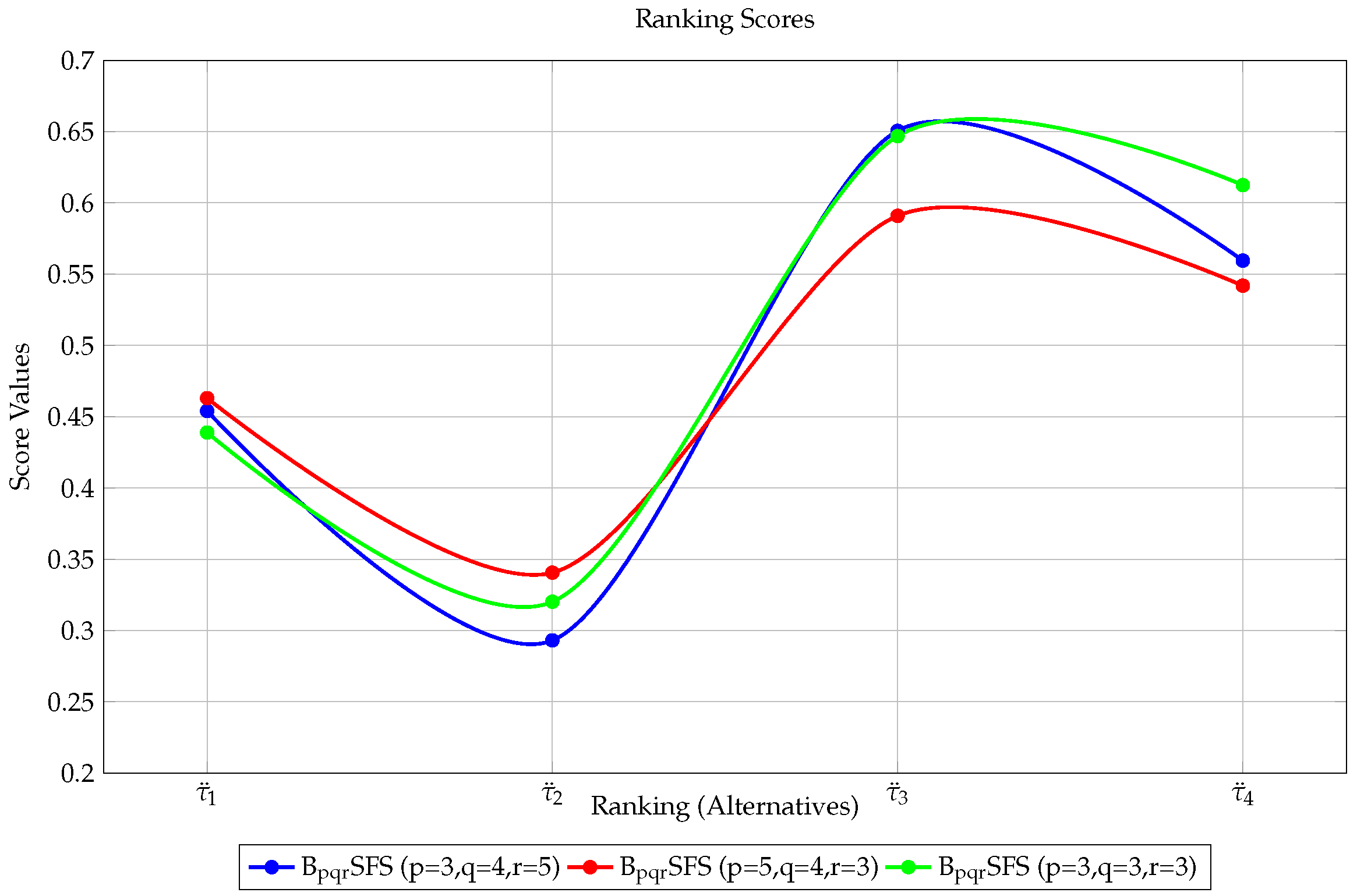
7. Sensitivity Analysis
8. Comparative Analysis
9. Conclusions
Author Contributions
Funding
Institutional Review Board Statement
Informed Consent Statement
Data Availability Statement
Acknowledgments
Conflicts of Interest
Appendix A. Proof
References
- Zadeh, L. Fuzzy sets. Inf. Control 1965, 8, 338–353. [Google Scholar]
- Atanassov, K.T. Intuitionistic fuzzy sets. Fuzzy Sets Syst. 1986, 20, 87–96. [Google Scholar]
- Yager, R.R. Pythagorean fuzzy subsets. In Proceedings of the 2013 joint IFSA world congress and NAFIPS annual meeting (IFSA/NAFIPS), Edmonton, AB, Canada, 24–28 June 2013; IEEE: Piscataway, NJ, USA, 2013; pp. 57–61. [Google Scholar]
- Yager, R.R. Generalized orthopair fuzzy sets. IEEE Trans. Fuzzy Syst. 2016, 25, 1222–1230. [Google Scholar] [CrossRef]
- Dounis, A.; Stefopoulos, A. Intelligent Medical Diagnosis Reasoning Using Composite Fuzzy Relation, Aggregation Operators and Similarity Measure of q-Rung Orthopair Fuzzy Sets. Appl. Sci. 2023, 13, 12553. [Google Scholar] [CrossRef]
- Seikh, M.R.; Mandal, U. Multiple attribute group decision making based on quasirung orthopair fuzzy sets: Application to electric vehicle charging station site selection problem. Eng. Appl. Artif. Intell. 2022, 115, 105299. [Google Scholar] [CrossRef]
- Ibrahim, H.Z.; Alshammari, I. n,m-Rung orthopair fuzzy sets with applications to multicriteria decision making. IEEE Access 2022, 10, 99562–99572. [Google Scholar]
- Cuong, B.C.; Kreinovich, V. Picture fuzzy sets. J. Comput. Sci. Cybern. 2014, 30, 409–420. [Google Scholar]
- Mahmood, T.; Ullah, K.; Khan, Q.; Jan, N. An approach toward decision-making and medical diagnosis problems using the concept of spherical fuzzy sets. Neural Comput. Appl. 2019, 31, 7041–7053. [Google Scholar]
- Kutlu Gündoğdu, F.; Kahraman, C. Spherical fuzzy sets and spherical fuzzy TOPSIS method. J. Intell. Fuzzy Syst. 2019, 36, 337–352. [Google Scholar]
- Ullah, K.; Garg, H.; Mahmood, T.; Jan, N.; Ali, Z. Correlation coefficients for T-spherical fuzzy sets and their applications in clustering and multi-attribute decision making. Soft Comput. 2020, 24, 1647–1659. [Google Scholar]
- Ali, J.; Naeem, M. r,s,t-spherical fuzzy VIKOR method and its application in multiple criteria group decision making. IEEE Access 2023, 11, 46454–46475. [Google Scholar] [CrossRef]
- Rahim, M.; Amin, F.; Tag Eldin, E.M.; Khalifa, A.E.W.; Ahmad, S. p,q-Spherical fuzzy sets and their aggregation operators with application to third-party logistic provider selection. J. Intell. Fuzzy Syst. 2024, 46, 505–528. [Google Scholar] [CrossRef]
- Rahim, M.; Ahmad, S.; Bajri, S.A.; Alharbi, R.; Khalifa, H.A.E.W. Confidence Levels-Based p,q,r–Spherical Fuzzy Aggregation Operators and Their Application in Selection of Solar Panels. IEEE Access 2024, 12, 57863–57878. [Google Scholar] [CrossRef]
- Kang, L.; Khan, S.; Rahim, M.; Shah, K.; Abdeljawad, T. Development p,q,r–Spherical Fuzzy Einstein Aggregation Operators: Application in Decision-Making in Logo Design. IEEE Access 2024, 12, 68393–68409. [Google Scholar] [CrossRef]
- Karaaslan, F.; Karamaz, F. Interval-valued (p,q,r)-spherical fuzzy sets and their applications in MCGDM and MCDM based on TOPSIS method and aggregation operators. Expert Syst. Appl. 2024, 255, 124575. [Google Scholar] [CrossRef]
- Ezhilmaran, D.; Sankar, K. Morphism of bipolar intuitionistic fuzzy graphs. J. Discret. Math. Sci. Cryptogr. 2015, 18, 605–621. [Google Scholar] [CrossRef]
- Mohana, K.; Jansi, R. Bipolar Pythagorean fuzzy sets and their application based on multi-criteria decision-making problems. Int. J. Res. Advent Technol. 2018, 6, 3754–3764. [Google Scholar]
- Palanikumar, M.; Iampan, A. Novel approach to decision making based on type-II generalized fermatean bipolar fuzzy soft sets. Int. J. Innov. Comput. Inf. Control 2022, 18, 769–781. [Google Scholar]
- Li, J.; Yüksel, S.; Dınçer, H.; Mikhaylov, A.; Barykin, S.E. Bipolar q-ROF hybrid decision making model with golden cut for analyzing the levelized cost of renewable energy alternatives. IEEE Access 2022, 10, 42507–42517. [Google Scholar] [CrossRef]
- Ibrahim, H.Z. Multi-attribute group decision-making based on bipolar n,m-rung orthopair fuzzy sets. Granul. Comput. 2023, 8, 1819–1836. [Google Scholar] [CrossRef]
- Princy, R.; Mohana, K. Spherical bipolar fuzzy sets and its application in multi criteria decision making problem. J. New Theory 2019, 32, 58–70. [Google Scholar]
- Wang, H.; Saad, M.; Karamti, H.; Garg, H.; Rafiq, A. An Approach Toward Pattern Recognition and Decision-Making Using the Concept of Bipolar T-Spherical Fuzzy Sets. Int. J. Fuzzy Syst. 2023, 25, 2649–2664. [Google Scholar] [CrossRef]
- Riaz, M.; Garg, H.; Athar Farid, H.M.; Chinram, R. Multi-criteria decision making based on bipolar picture fuzzy operators and new distance measures. Comput. Model. Eng. Sci. 2021, 127, 771–800. [Google Scholar]
- Ashraf, S.; Abdullah, S.; Mahmood, T.; Ghani, F.; Mahmood, T. Spherical fuzzy sets and their applications in multi-attribute decision making problems. J. Intell. Fuzzy Syst. 2019, 36, 2829–2844. [Google Scholar]
- Senapati, T.; Yager, R.R. Fermatean fuzzy sets. J. Ambient Intell. Humaniz. Comput. 2020, 11, 663–674. [Google Scholar]
- Hwang, C.L.; Yoon, K. Methods for multiple attribute decision making. In Multiple Attribute Decision Making: Methods and Applications A State-of-the-Art Survey; Springer: Berlin/Heidelberg, Germany, 1981; Volume 186, pp. 58–191. [Google Scholar]
- Yoon, K. A reconciliation among discrete compromise solutions. J. Oper. Res. Soc. 1987, 38, 277–286. [Google Scholar]
- Hwang, C.L.; Lai, Y.J.; Liu, T.Y. A new approach for multiple objective decision making. Comput. Oper. Res. 1993, 20, 889–899. [Google Scholar]
- El Alaoui, M. Fuzzy TOPSIS: Logic, Approaches, and Case Studies; CRC Press: Boca Raton, FL, USA, 2021. [Google Scholar]
- Maldonado-Macías, A.; Alvarado, A.; García, J.L.; Balderrama, C.O. Intuitionistic fuzzy TOPSIS for ergonomic compatibility evaluation of advanced manufacturing technology. Int. J. Adv. Manuf. Technol. 2014, 70, 2283–2292. [Google Scholar]
- Junior, F.R.L.; Osiro, L.; Carpinetti, L.C.R. A comparison between Fuzzy AHP and Fuzzy TOPSIS methods to supplier selection. Appl. Soft Comput. 2014, 21, 194–209. [Google Scholar]
- Yilmaz, I.; Ecemis Yilmaz, H.K. A consensus framework for evaluating dispute resolution alternatives in international law using an interval-valued type-2 fuzzy TOPSIS approach. Appl. Sci. 2024, 14, 11046. [Google Scholar] [CrossRef]
- Jin, J.; Zhao, P.; You, T. Picture fuzzy TOPSIS method based on CPFRS model: An application to risk management problems. Sci. Program. 2021, 2021, 6628745. [Google Scholar] [CrossRef]
- Akram, M.; Shumaiza; Arshad, M. Bipolar fuzzy TOPSIS and bipolar fuzzy ELECTRE-I methods to diagnosis. Comput. Appl. Math. 2020, 39, 1–21. [Google Scholar] [CrossRef]
- Calvo, T.; Mayor, G.; Mesiar, R. Aggregation operators, Studies Fuzziness Soft Computing 97. Phys. Heidelb. 2002. [Google Scholar]
- Grabisch, M.; Marichal, J.L.; Mesiar, R.; Pap, E. Aggregation Functions, Cambridge University Press. In Proceedings of the 2008 6th International Symposium on Intelligent Systems and Informatics, Subotica, Serbia, 26–27 September 2008; IEEE: Piscataway, NJ, USA, 2008; pp. 1–7. [Google Scholar]
- Yager, R.R.; Kacprzyk, J. The Ordered Weighted Averaging Operators: Theory and Applications; Springer Science & Business Media: Berlin/Heidelberg, Germany, 2012. [Google Scholar]
- Xu, Z.; Yager, R.R. Some geometric aggregation operators based on intuitionistic fuzzy sets. Int. J. Gen. Syst. 2006, 35, 417–433. [Google Scholar] [CrossRef]
- Xu, Z. Intuitionistic fuzzy aggregation operators. IEEE Trans. Fuzzy Syst. 2007, 15, 1179–1187. [Google Scholar]
- Wei, G. Picture fuzzy aggregation operators and their application to multiple attribute decision making. J. Intell. Fuzzy Syst. 2017, 33, 713–724. [Google Scholar] [CrossRef]
- Garg, H.; Ullah, K.; Mahmood, T.; Hassan, N.; Jan, N. T-spherical fuzzy power aggregation operators and their applications in multi-attribute decision making. J. Ambient Intell. Humaniz. Comput. 2021, 12, 9067–9080. [Google Scholar] [CrossRef]
- Akram, M.; Dudek, W.A.; Ilyas, M.F. Group decision making based on Pythagorean fuzzy TOPSIS method. Int. J. Intell. Syst. 2019, 34, 1455–1475. [Google Scholar] [CrossRef]
- Gul, M.; Lo, H.W.; Yucesan, M. Fermatean fuzzy TOPSIS-based approach for occupational risk assessment in manufacturing. Complex Intell. Syst. 2021, 7, 2635–2653. [Google Scholar] [CrossRef]
- Pınar, A.; Rouyendegh, B.D.; Özdemir, Y.S. q-Rung orthopair fuzzy TOPSIS method for green supplier selection problem. Sustainability 2021, 13, 985. [Google Scholar] [CrossRef]


| Model | MD | NMD | ¬MD | FSDP * | Bipolarity |
|---|---|---|---|---|---|
| FS [1] | Yes | No | No | No | No |
| IFS [2] | Yes | No | Yes | No | No |
| PyFS [3] | Yes | No | Yes | No | No |
| FFS [26] | Yes | No | Yes | No | No |
| q-ROFS [4] | Yes | No | Yes | No | No |
| mn-ROFS [7] | Yes | No | Yes | Yes | No |
| PFS [8] | Yes | Yes | Yes | No | No |
| SFS [9,25] | Yes | Yes | Yes | No | No |
| T-SFS [9] | Yes | Yes | Yes | No | No |
| pqr-SFS [12,13] | Yes | Yes | Yes | Yes | No |
| BIFS [17] | Yes | No | Yes | No | Yes |
| BPyFS [18] | Yes | No | Yes | No | Yes |
| FBFS [19] | Yes | No | Yes | No | Yes |
| Bmn-ROFS [21] | Yes | No | Yes | Yes | Yes |
| BPFS [24] | Yes | Yes | Yes | No | Yes |
| SBFS [22] | Yes | Yes | Yes | No | Yes |
| BT-SFS [23] | Yes | Yes | Yes | No | Yes |
| Proposed | Yes | Yes | Yes | Yes | Yes |
| Cost | Quality | Delivery Time | |
|---|---|---|---|
| Cost | Quality | Delivery Time | |
|---|---|---|---|
| Cost C1 | Quality C2 | Delivery Time C3 | |
|---|---|---|---|
| {0.0018, 0.1585, 0.9524, −0.3245,−0.0716, −0.0083} | {0.3548, 0.3981, 0.3092, −0.5357,−0.0007, −0.0907} | {0.0047, 0.8326, 0.8841, −0.631,−0.0017, −0.1279} | |
| {0.0047, 0.246, 0.9317, −0.2091,−0.1272, −0.0333} | {0.3876, 0.5253, 0.3492, −0.4922,−0.008, −0.0035} | {0.0258, 0.6178, 0.9258, −0.6034,−0.0354, −0.0742} | |
| {0.0018, 0.1585, 0.9456, −0.6178,−0.0007,−0.0141} | {0.3655, 0.246, 0.5544, −0.5357,−0.0003,−0.0101} | {0.0169, 0.631, 0.939, −0.8152,−0.0006,−0.0351} | |
| {0.0012, 0.3817, 0.9352, −0.634,−0.0013, −0.048} | {0.5129, 0.3245, 0.2512, −0.4282,−0.0039, −0.2082} | {0.0058, 0.6178, 0.9587, −0.7638,−0.0006,−0.0104} |
| Ideal Solutions | Cost C1 | Quality C2 | Delivery Time C3 |
|---|---|---|---|
| BpqrSFPIS | {0.0047, 0.1585, 0.91, −0.634, −0.0007, −0.0083} | {0.5129, 0.246, 0.1585, −0.5357, −0.0003, −0.0035} | {0.0258, 0.6178, 0.8841, −0.8152, −0.0006, −0.0104} |
| BpqrSFNIS | {0.0012, 0.1585, 0.9371, −0.2091, −0.0007, −0.048} | {0.3548, 0.246, 0.4555, −0.4282, −0.0003, −0.2082} | {0.0047, 0.6178, 0.9587, −0.6034, −0.0006, −0.1279} |
| Alternatives | ||
|---|---|---|
| Alternatives | |
|---|---|
| Alternatives | |
|---|---|
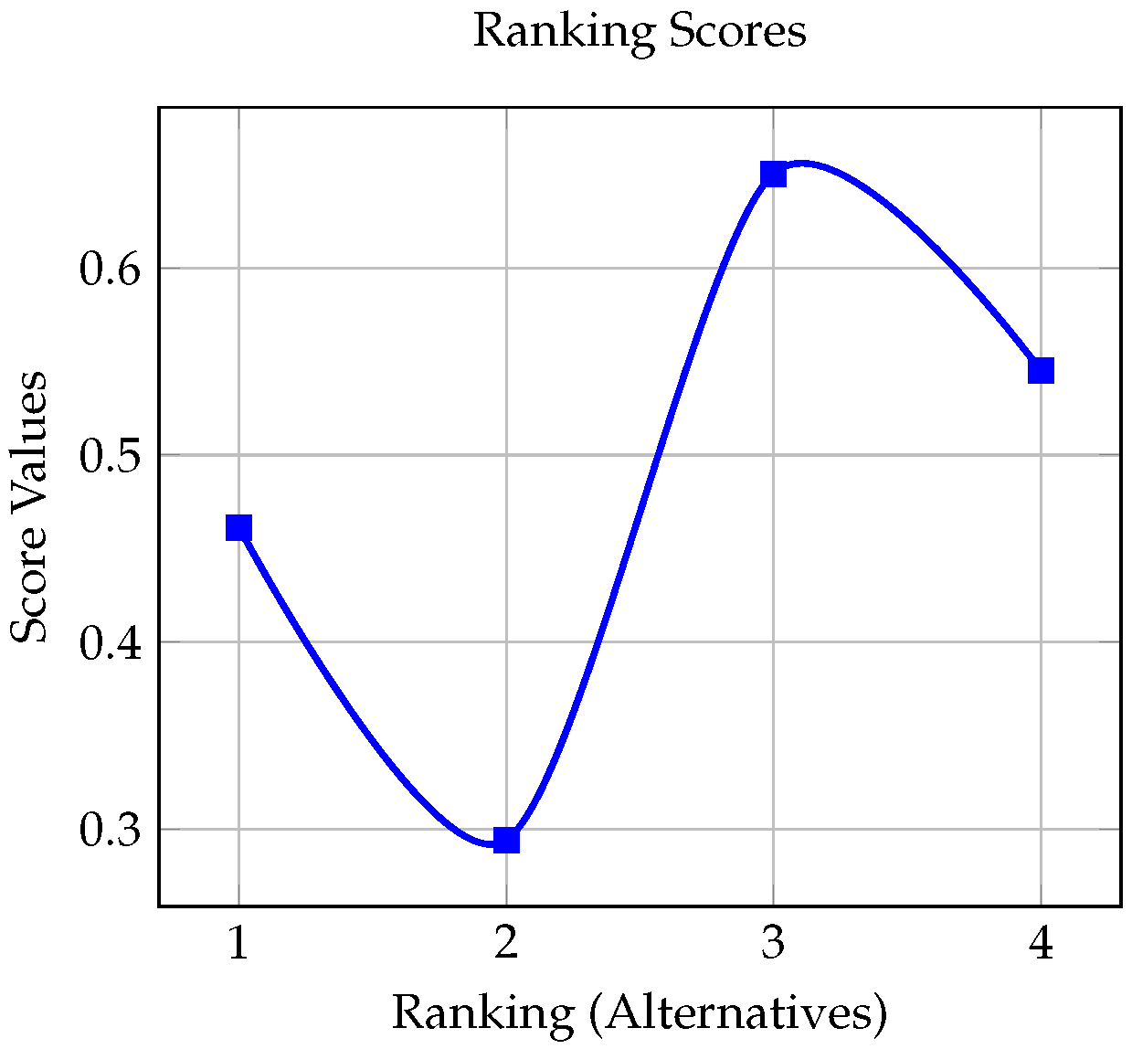
| SFS | Ranking Results | ||||
|---|---|---|---|---|---|
| 0.454 | 0.2931 | 0.6215 | 0.5595 | ||
| 0.463 | 0.3406 | 0.5909 | 0.5419 | ||
| 0.4389 | 0.3202 | 0.6468 | 0.6125 |
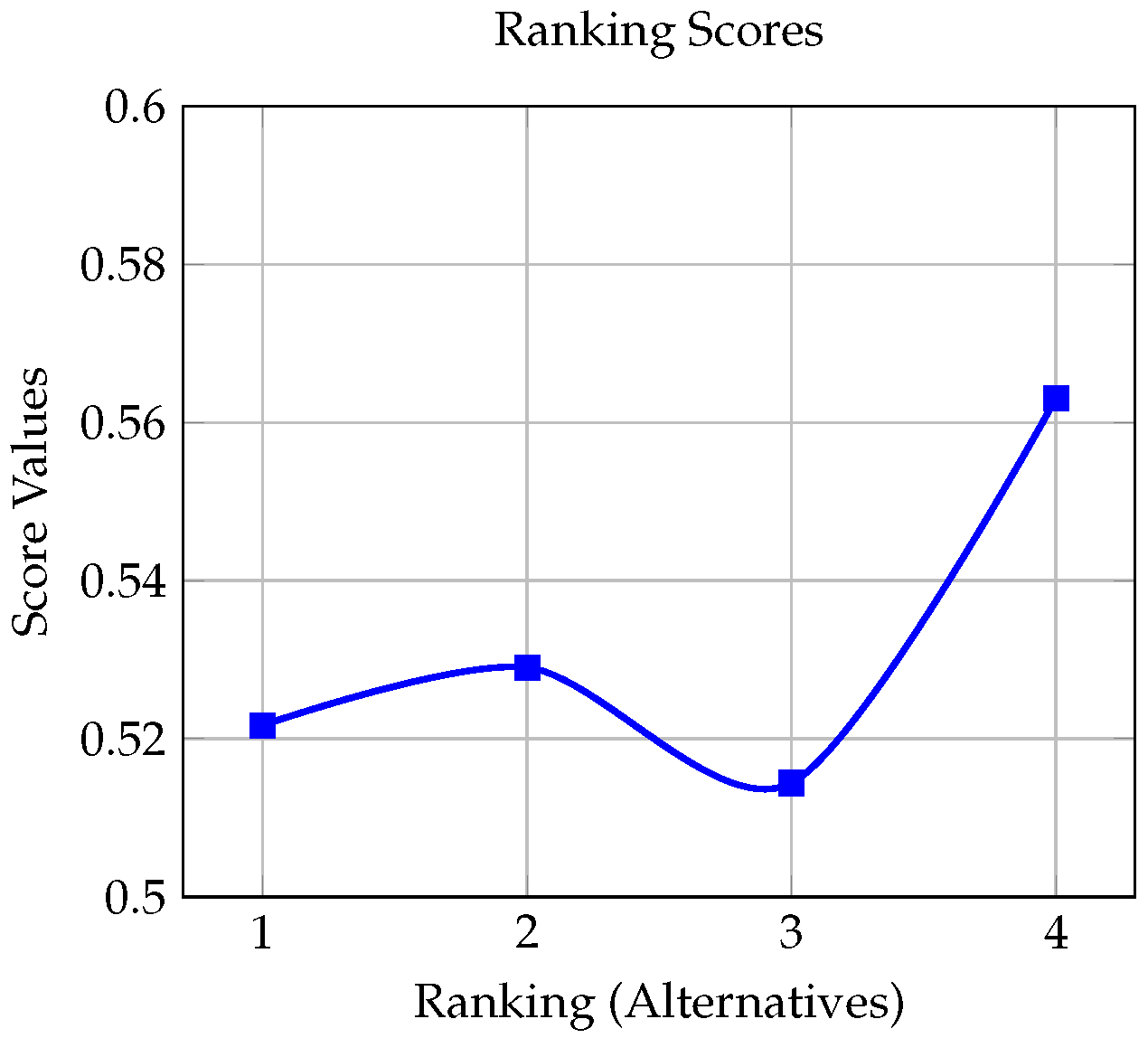
| SFWA | Ranking Results | ||||
|---|---|---|---|---|---|
| 0.605 | 0.6205 | 0.5996 | 0.6793 | ||
| 0.5494 | 0.561 | 0.5493 | 0.6193 | ||
| 0.5722 | 0.5859 | 0.5732 | 0.6468 | ||
| 0.6045 | 0.6194 | 0.5938 | 0.679 | ||
| 0.6503 | 0.6699 | 0.6244 | 0.71 | ||
| 0.605 | 0.6206 | 0.601 | 0.6792 | ||
| 0.5234 | 0.5315 | 0.5244 | 0.5794 | ||
| 0.5496 | 0.5615 | 0.5527 | 0.6196 | ||
| 0.5025 | 0.5044 | 0.503 | 0.524 |
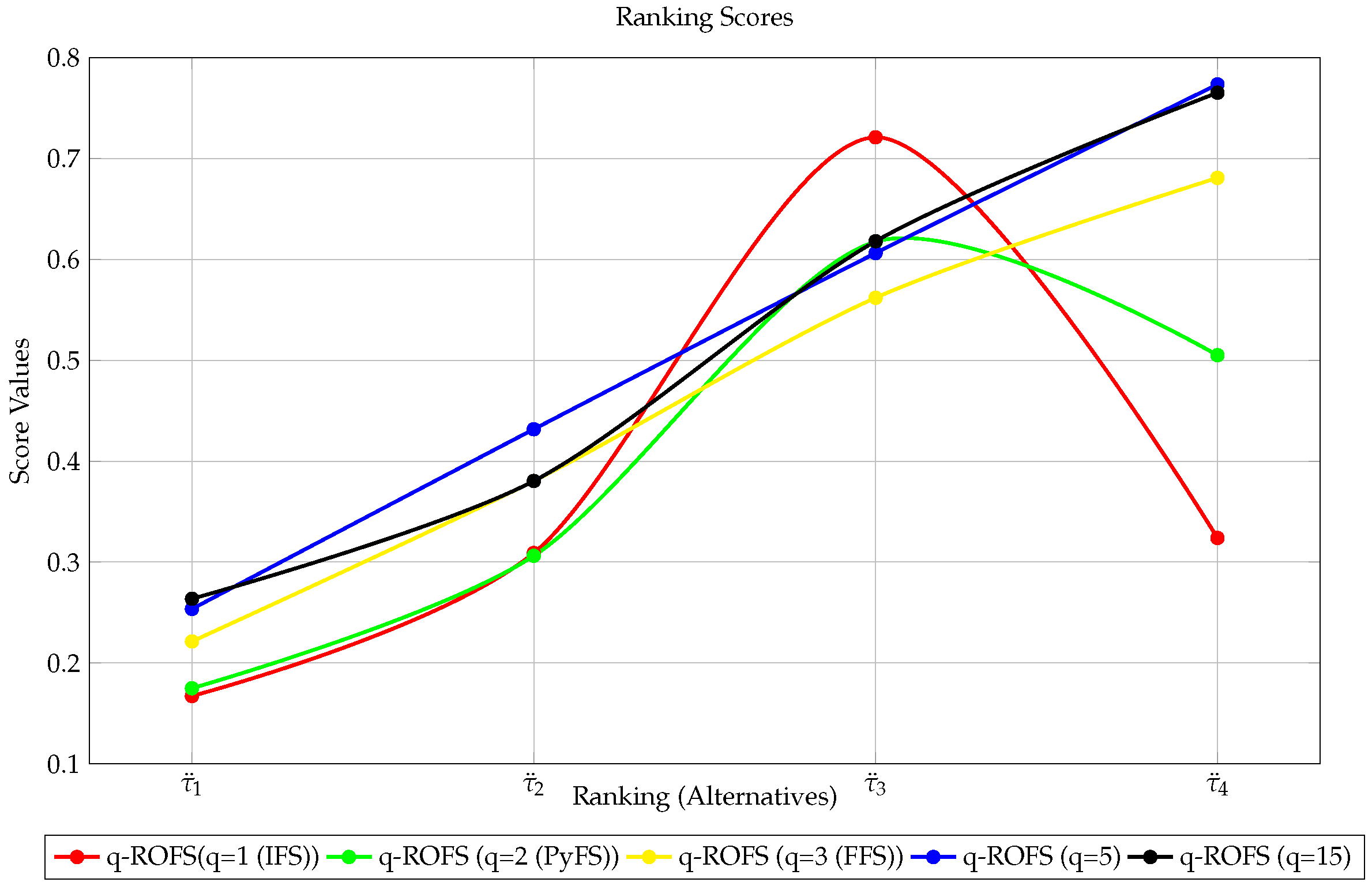
| q-ROFS | Ranking Results | ||||
|---|---|---|---|---|---|
| 0.1672 | 0.309 | 0.7211 | 0.3239 | ||
| 0.1749 | 0.3062 | 0.6176 | 0.5051 | ||
| 0.2213 | 0.3804 | 0.562 | 0.6809 | ||
| 0.2535 | 0.4317 | 0.6063 | 0.7735 | ||
| 0.2636 | 0.3804 | 0.6181 | 0.7653 |
| BT-SFS | Ranking Results | ||||
|---|---|---|---|---|---|
| 0.474 | 0.4438 | 0.6549 | 0.5778 | ||
| 0.3661 | 0.4233 | 0.7135 | 0.6862 | ||
| 0.4406 | 0.3051 | 0.6776 | 0.5063 | ||
| 0.3557 | 0.50008 | 0.659 | 0.6084 |
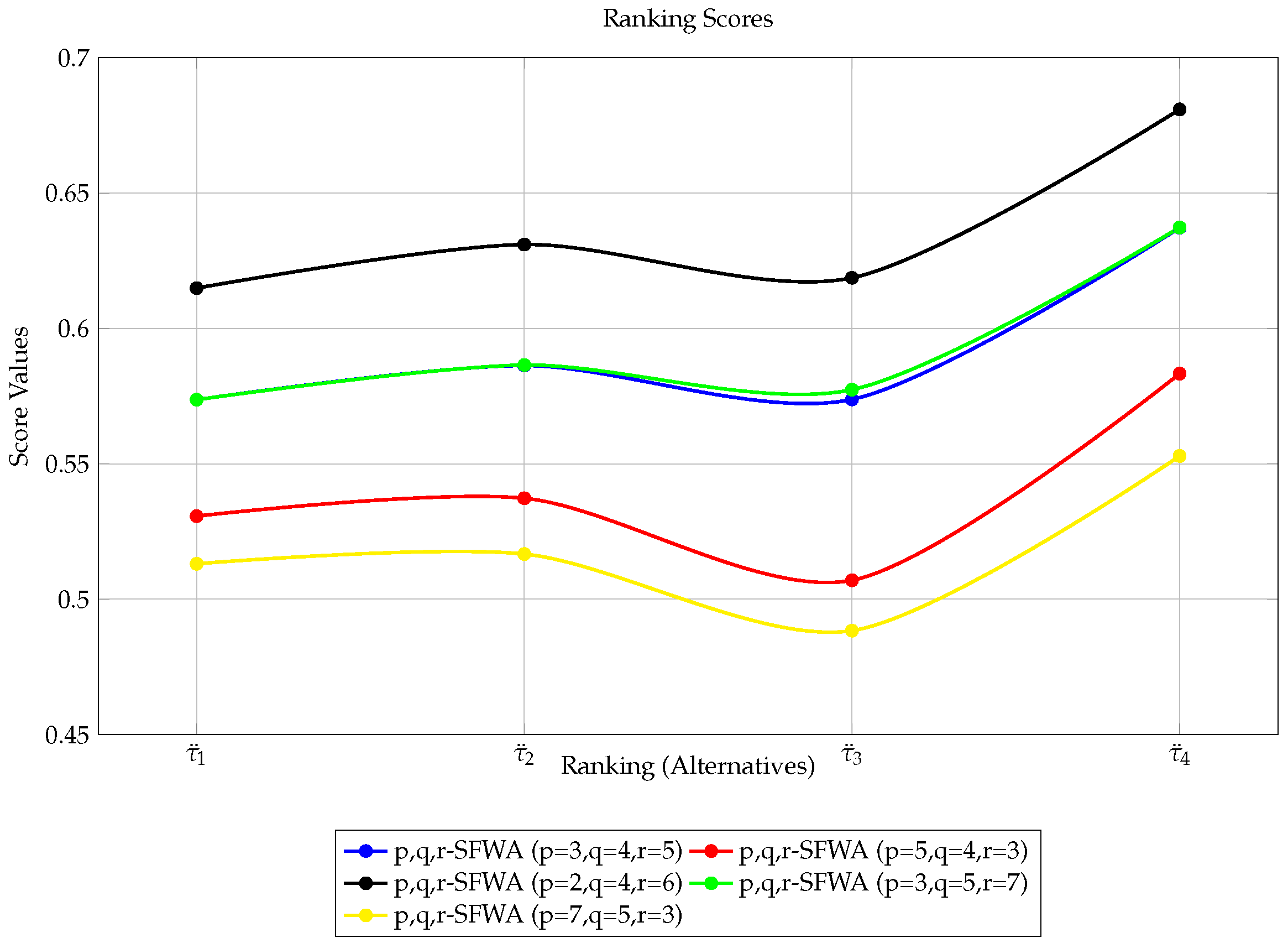
| pqr-SFWA | Ranking Results | ||||
|---|---|---|---|---|---|
| 0.5737 | 0.5863 | 0.5738 | 0.6372 | ||
| 0.5307 | 0.5373 | 0.507 | 0.5833 | ||
| 0.6149 | 0.631 | 0.6187 | 0.6809 | ||
| 0.5737 | 0.5865 | 0.5774 | 0.6373 | ||
| 0.5131 | 0.5167 | 0.4884 | 0.5529 |
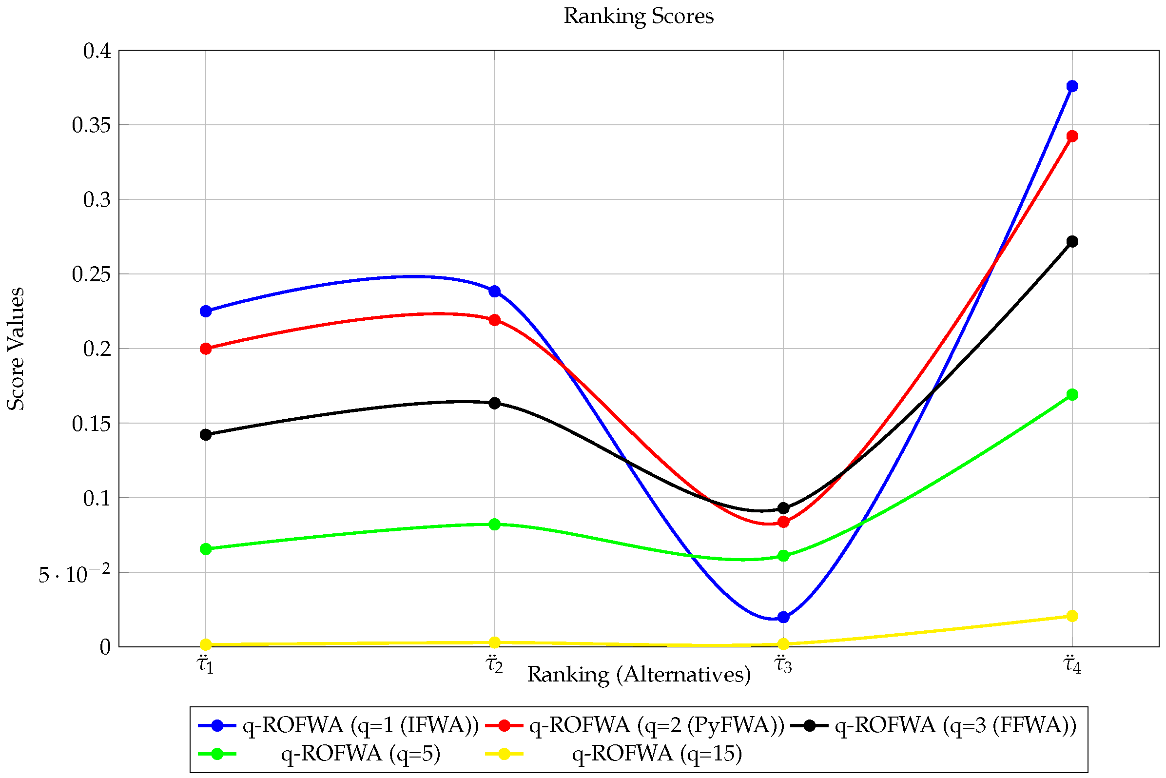
| q-ROFWA | Ranking Results | ||||
|---|---|---|---|---|---|
| 0.225 | 0.2383 | 0.0199 | 0.3759 | ||
| 0.1999 | 0.2191 | 0.0838 | 0.3424 | ||
| 0.1422 | 0.1633 | 0.093 | 0.2718 | ||
| 0.0656 | 0.0821 | 0.0611 | 0.1691 | ||
| 0.0015 | 0.0029 | 0.0019 | 0.0207 |
| -ROFWA | Ranking Results | ||||
|---|---|---|---|---|---|
| 0.1914 | 0.176 | −0.0544 | 0.2533 | ||
| 0.094 | 0.0913 | −0.0183 | 0.1585 | ||
| 0.0379 | 0.0424 | −0.0035 | 0.0818 | ||
| 0.0056 | 0.0087 | 0.0007 | 0.0201 | ||
| 0.000024 | 0.000003 | 0.00000052 | 0.0000005 |
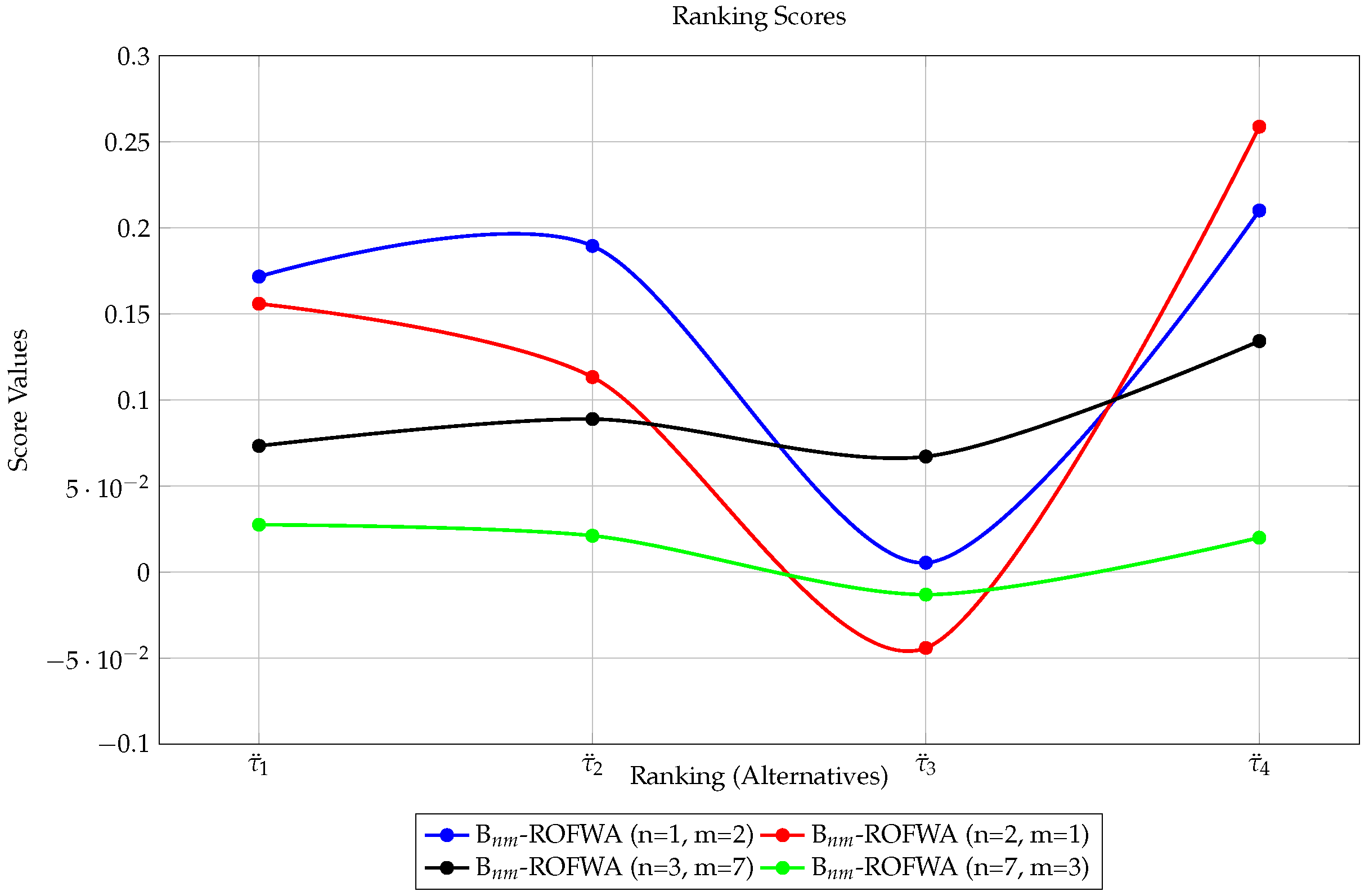
| -ROFWA | Ranking Results | ||||
|---|---|---|---|---|---|
| 0.1718 | 0.1896 | 0.0055 | 0.2102 | ||
| 0.156 | 0.1134 | −0.044 | 0.2589 | ||
| 0.0734 | 0.089 | 0.0672 | 0.1343 | ||
| 0.0276 | 0.0212 | −0.013 | 0.0201 |
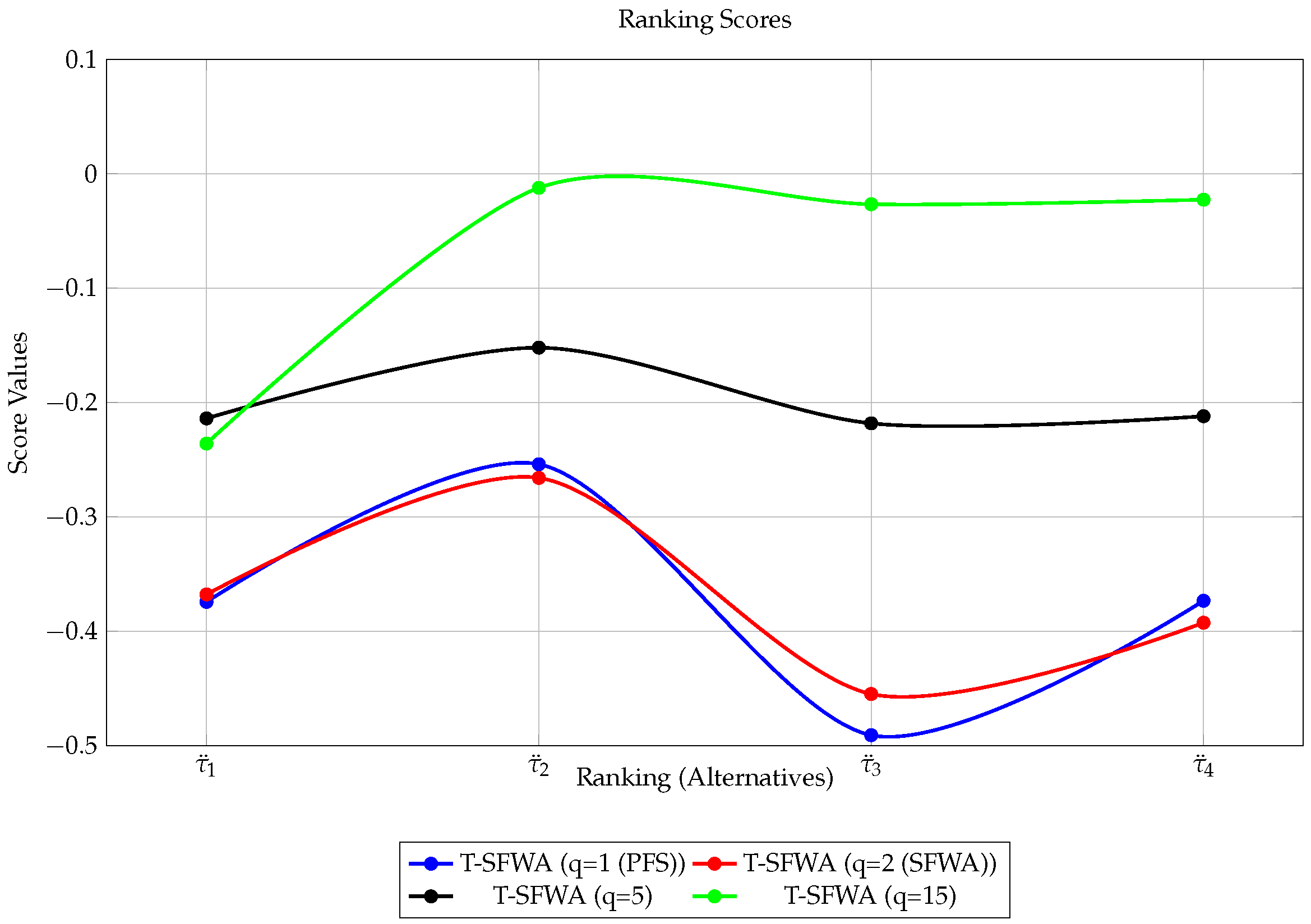
| T-SFWA | Ranking Results | ||||
|---|---|---|---|---|---|
| −0.3743 | −0.254 | −0.4908 | −0.3733 | ||
| −0.3678 | −0.2659 | −0.4548 | −0.3925 | ||
| −0.2139 | −0.1521 | −0.2182 | −0.212 | ||
| −0.2359 | −0.0124 | −0.0267 | −0.0227 |
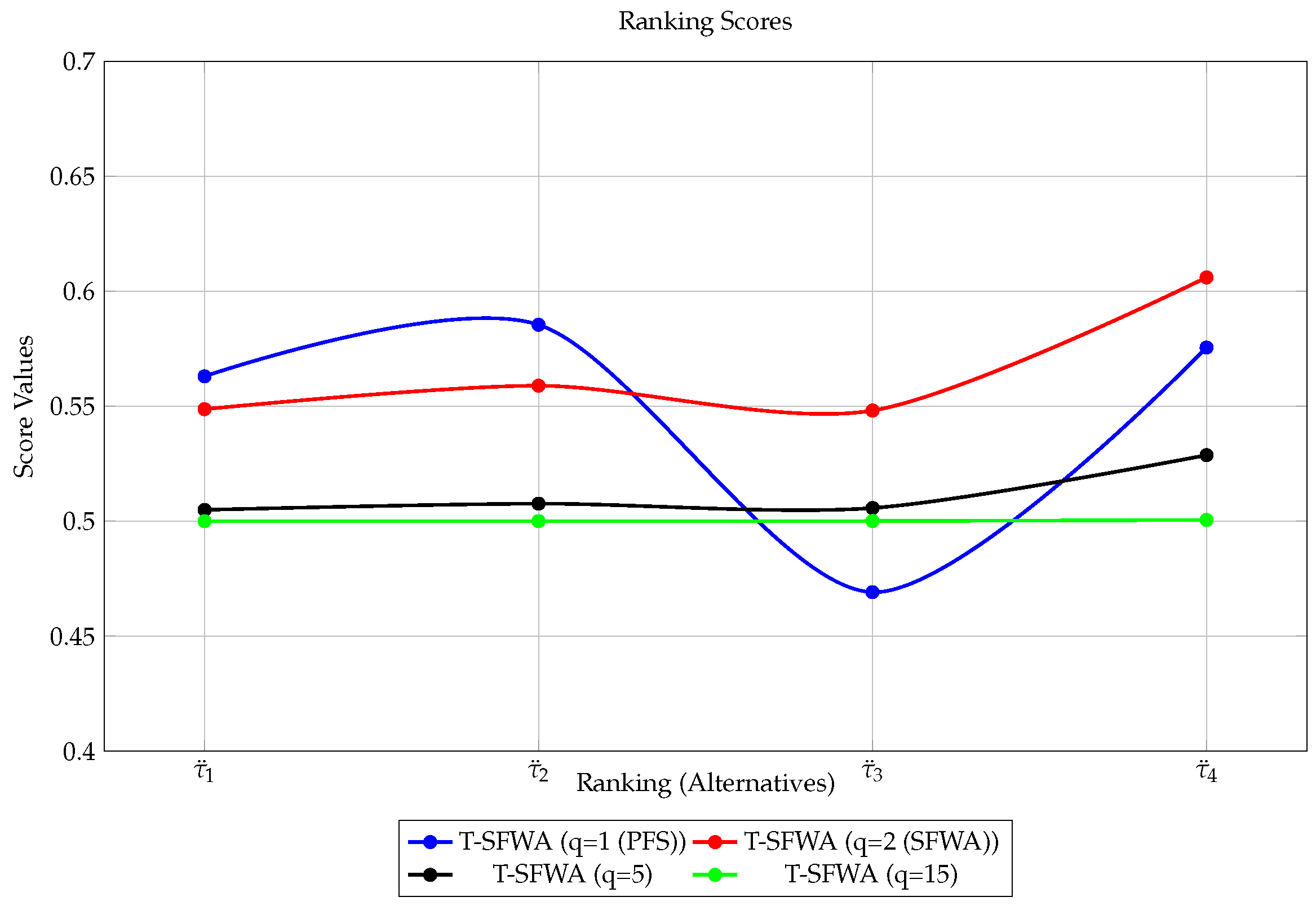
| BT-SFWA | Ranking Results | ||||
|---|---|---|---|---|---|
| 0.563 | 0.5854 | 0.4691 | 0.5755 | ||
| 0.5487 | 0.5589 | 0.5481 | 0.606 | ||
| 0.5049 | 0.5076 | 0.5057 | 0.5287 | ||
| 0.500003 | 0.50001 | 0.500005 | 0.50052 |
| Method | Parameter(s) | Ranking Results | Optimal Alternative |
|---|---|---|---|
| IFS TOPSIS [31] | n/a | ||
| PyFS TOPSIS [43] | n/a | ||
| FFS TOPSIS [44] | n/a | ||
| q-ROF TOPSIS [45] | |||
| BT-SFS TOPSIS [23] | |||
| SF TOPSIS (proposed) | |||
| q-ROFWA [20] | |||
| T-SFWAO [42] | |||
| pqr-SFWAO [12] | |||
| -ROFWAO [20] | |||
| -ROFWAO [21] | |||
| BT-SFWA [23] | |||
| SFWAO (proposed) | |||
Disclaimer/Publisher’s Note: The statements, opinions and data contained in all publications are solely those of the individual author(s) and contributor(s) and not of MDPI and/or the editor(s). MDPI and/or the editor(s) disclaim responsibility for any injury to people or property resulting from any ideas, methods, instructions or products referred to in the content. |
© 2025 by the authors. Licensee MDPI, Basel, Switzerland. This article is an open access article distributed under the terms and conditions of the Creative Commons Attribution (CC BY) license (https://creativecommons.org/licenses/by/4.0/).
Share and Cite
Ameen, Z.A.; Salih, H.F.M.; Alajlan, A.I.; Mohammed, R.A.; Asaad, B.A. Enhanced MCDM Based on the TOPSIS Technique and Aggregation Operators Under the Bipolar pqr-Spherical Fuzzy Environment: An Application in Firm Supplier Selection. Appl. Sci. 2025, 15, 3597. https://doi.org/10.3390/app15073597
Ameen ZA, Salih HFM, Alajlan AI, Mohammed RA, Asaad BA. Enhanced MCDM Based on the TOPSIS Technique and Aggregation Operators Under the Bipolar pqr-Spherical Fuzzy Environment: An Application in Firm Supplier Selection. Applied Sciences. 2025; 15(7):3597. https://doi.org/10.3390/app15073597
Chicago/Turabian StyleAmeen, Zanyar A., Hariwan Fadhil M. Salih, Amlak I. Alajlan, Ramadhan A. Mohammed, and Baravan A. Asaad. 2025. "Enhanced MCDM Based on the TOPSIS Technique and Aggregation Operators Under the Bipolar pqr-Spherical Fuzzy Environment: An Application in Firm Supplier Selection" Applied Sciences 15, no. 7: 3597. https://doi.org/10.3390/app15073597
APA StyleAmeen, Z. A., Salih, H. F. M., Alajlan, A. I., Mohammed, R. A., & Asaad, B. A. (2025). Enhanced MCDM Based on the TOPSIS Technique and Aggregation Operators Under the Bipolar pqr-Spherical Fuzzy Environment: An Application in Firm Supplier Selection. Applied Sciences, 15(7), 3597. https://doi.org/10.3390/app15073597