Automatic Detection and Unsupervised Clustering-Based Classification of Cetacean Vocal Signals ^†

Abstract

In the ocean environment, passive acoustic monitoring (PAM) is an important technique for the surveillance of cetacean species. Manual detection for a large amount of PAM data is inefficient and time-consuming. To extract useful features from a large amount of PAM data for classifying different cetacean species, we propose an automatic detection and unsupervised clustering-based classification method for cetacean vocal signals. This paper overcomes the limitations of the traditional threshold-based method, and the threshold is set adaptively according to the mean value of the signal energy in each frame. Furthermore, we also address the problem of the high cost of data training and labeling in deep-learning-based methods by using the unsupervised clustering-based classification method. Firstly, the automatic detection method extracts vocal signals from PAM data and, at the same time, removes clutter information. Then, the vocal signals are analyzed for classification using a clustering algorithm. This method grabs the acoustic characteristics of vocal signals and distinguishes them from environmental noise. We process 194 audio files in a total of 25.3 h of vocal signal from two marine mammal public databases. Five kinds of vocal signals from different cetaceans are extracted and assembled to form 8 datasets for classification. The verification experiments were conducted on four clustering algorithms based on two performance metrics. The experimental results confirm the effectiveness of the proposed method. The proposed method automatically removes about 75% of clutter data from 1581.3MB of data in audio files and extracts 75.75 MB of the features detected by our algorithm. Four classical unsupervised clustering algorithms are performed on the datasets we made for verification and obtain an average accuracy rate of 84.83%.

1. Introduction

Many cetacean species are currently considered endangered [1]. The surveillance and protection of cetaceans is an important issue and has attracted wide research attention. Nowadays, an effective way of studying cetaceans’ presences and acoustic behaviors is through passive acoustic monitoring (PAM) [2]. PAM is more effective than active monitoring in some way. For example, it provides a non-invasive, cost-effective, and environmentally friendly way to study cetaceans over large areas and extended periods. It allows researchers to gather detailed, species-specific data without disturbing the animals. However, PAM also has some limitations and disadvantages. The implementation of PAM systems depends very much on their application and operational circumstances. PAM activity results are not easily adapted directly to standard analysis tools that have proven successful in visually based active monitoring [3]. Since many cetacean species mainly rely on vocal signals such as echolocation click, whistle, and burst pulse for foraging, positioning, and communication, their vocal signals have become the most common and important research object for studying cetaceans [4,5]. However, passive acoustic monitoring of cetaceans faces some challenges [2,3]. Firstly, the hydrophones in PAM collect data over many months and produce a large volume of data. Many of the underwater acoustic data contain noise from the ocean environment, which is hard to distinguish from the signals we are interested in [6]. Furthermore, some cetacean vocal signals are broadband signals, which usually only last a few seconds or minutes [7]. Consequently, the transient nature of the signals and the high variability in cetacean sounds at the individual level make it difficult to recognize the different species of cetaceans through the collected waveform. To tackle this difficulty, we shall investigate more effective ways to detect and classify vocal signals of cetaceans automatically.

Early research on cetacean vocal detection focused on threshold-based methods [8,9,10,11]. These methods compute the standard deviation or root mean square of signals’ parameters such as the peak frequency, frequency band, or width of the principal spectral peak and set a proper threshold. Detection is triggered when the signal values are above the threshold. Kandia et al. [9] constructed a Teager-Kaiser energy operator (TKEO) to detect sperm whale clicks, where the peak picking algorithm and forward–backward search algorithm are applied to detect the time instant of the highest peak as a vocal sound. These two methods only determine the existence of vocal signals. After detection, they still require manual processing to locate the vocal signals. The energy ratio mapping algorithm (ERMA) [11] was developed to improve the performance of energy-based detection of odontocete vocal signals. It evaluates the frequency bands of data to detect vocal signals through a noise-adaptive threshold in the TKEO function. However, its extension to cetacean vocal signals is not straightforward due to the short time duration of vocal signals. Generally, the threshold-based detection technique has shown its effectiveness in cetacean vocal detection. However, it is difficult to decide on a proper threshold, which usually requires some adaptive or self-learning technique due to the time-varying environment.

Automatic classification of the cetaceans’ vocal signals is also an important issue. With the development of artificial intelligence technology, machine learning methods have been applied to many different fields with no exception to the classification of cetacean vocal signals [12,13]. There are two main kinds of machine learning methods used in this task: supervised and unsupervised learning. In supervised classification, a convolutional neural network (CNN) [14] is a popular tool for automatic cetacean classification [15,16,17]. Rasmussen et al. [17] combined rCNN (region-based convolutional neural network) and CNN networks to classify spectrograms created by fast Fourier transform (FFT) of fin whale and blue whale vocal signals and achieved a precision higher than 90%. In [15,16], the authors trained a CNN network to extract vocal signal features and predict the species of odontocetes for classification. Roch et al. [18,19] employed TKEO and cepstral analysis to construct feature vectors of odontocetes’ vocal signals and then train a Gaussian mixture model (GMM) and support vector machines (SVMs) model for classification of odontocetes, with 67–75% accuracy. Other supervised classification methods, e.g., K-nearest neighbors (KNN) method [20], feed-forward neural networks [21], and artificial neural network [22], have also been used in classifying the vocal signals of cetaceans. The supervised methods must label the vocal signals manually to generate the training data set. Moreover, they usually have large training datasets, which conflicts with the real-world situation of data deficiency. For instance, the CNN method [16] generates 4128 to 167,645 vocal samples for classification.

Thereby, unsupervised methods are used to reduce labeling burden and classify cetacean calls [5,23,24]. Clustering is the main and significant method in unsupervised frameworks. It groups data into clusters based on their internal characteristics information [25]. Li et al. [26] proposed a hybrid classifier with unsupervised clustering to classify beaked whale calls automatically. This method flags the energy-band spectral characteristics of whale calls. It utilizes a hierarchical cluster tree or dendrogram to cluster data into species-specific groups with a recall rate of 82.8% for Cuvier’s beaked whale and 77.9% for Gervais’. Reference [27] presents and evaluates several methods for automated species-level classification of vocal signals from three beaked whale species. Feature sets of three vocal types are selected for classification based on unsupervised step-wise discriminant analysis. The manually validated datasets of species-level BW vocal signals and unidentified dolphin vocal signals are used to evaluate six clustering algorithms, including k-means$++$ algorithm, Ward hierarchical clustering, and four graph-based clustering methods. In the unsupervised network-based classification [28], an unsupervised learning strategy associating the CW clustering algorithm with the pruned network was developed to identify dominant vocal types based on vocal spectral shape and inter-click interval (ICI) distributions computed by discrete Fourier transform (DFT). Manual removal of false positives is operated by an analyst using detEdit, a custom graphical user interface (GUI)-based tool. In deep embedded clustering (DEC), Reeves et al. [29] manually labeled a dataset for classifying simulated signals into fish and whale clusters. DEC, GMM, and conventional clustering were tested, and DEC achieved the highest accuracy of 77.5%. The unsupervised methods mentioned above can only distinguish several specific types of cetaceans’ vocal signals in small datasets and require manual operation to some extent.

In this paper, our key motivation is to pick up valuable data (i.e., cetacean sound) from real-world recorded signals, where only a small portion of the signals is valuable. Since all kinds of cetacean sounds are of interest, we consider different type of vocalizations from different cetacean species. By doing this, we build a data set of cetacean sounds that are valuable for future research. Further, unsupervised classification is applied to validate the effectiveness of our built data set.

This method mainly includes three parts: automatic detection, feature extraction, and unsupervised clustering-based classification. All the experiments are conducted in MATLAB R2016a with the program package “audio”. The workflow diagram for the whole process is shown in Figure 1.

1.1. Data Collection

The underwater acoustic data used are obtained from two open-source databases—Mobysound database (http://www.mobysound.org/ accessed on 1 January 2023) and Watkins Marine Mammal Sound database (https://cis.whoi.edu/science/B/whalesounds/index.cfm accessed on 1 January 2023). Mobysound database is a reference archive for studying the automatic recognition of marine mammal sounds [30]. The Mobysound database provides open-source information on different types of sounds from various species of marine mammals in a wide range of geographic areas. Watkins Marine Mammal Sound Database, built by William Watkins, is a resource that contains approximately 2000 unique recordings of more than 60 species of marine mammals [31]. The waveform of vocal signals was selected from five cetacean species, including common dolphin (Delphinus delphis), right whale (Eubalaena glacialis), Risso’s dolphin (Grampus griseus), pilot whale (Globicephala macrorhynchus), and beaked whale (Mesoplodon densirostris). The audio files of Blainville’s beaked whale (BW), pilot whale (PW), and Risso’s dolphin (RD) are from the 3rd International Workshop on Detection, Classification, Localization, and Density Estimation (DCLDE) of Marine Mammals using passive acoustics in Mobysound. Right whale (RW) upsweep sound and a set of background noise data with no whales come up from the 6th workshop in Mobysound. The audio files of common dolphins (CD) are from Watkins Marine Mammal Sound Database. The reason we chose these species is they are common species of cetaceans, and these species’ data are complete and adequate, so they are fit for our experiment requirements. Firstly, the amount of data is large enough that each species has a minimum duration of more than half an hour. Secondly, the recordings may include different types of vocal signals, such as echolocation click, whistle, and burst pulse. These recordings have been visually confirmed as originating from some specific single species, which means the vocal signals from a recording belong to the same species. According to the relative README files, it is known that each sound file is a single continuous recording—a sequence of digital samples from one or more hydrophones saved in WAVE format. In the same audio file, there are different types of vocalizations. The total data are contained within 194 waveform files of 25.3 h duration, or approximately 1.54 G of data. Nevertheless, due to ambient noise and non-stationary characteristics, the wave data in sound files cannot yet be utilized directly in automatic call recognition research. Consequently, automatic detection and feature extraction are essential for unsupervised classification.

The original data are collected using one recording configuration in or near one geographic area over one relatively short time span. Some details will vary from one sound dataset to another; for example, recorders of right whales were deployed in arrays of six or ten devices, a single channel having been stripped out and converted to 16 bit wav file format with a sample rate of 2 kHz. More details of other datasets can be found in the descriptions of databases in [30,31].

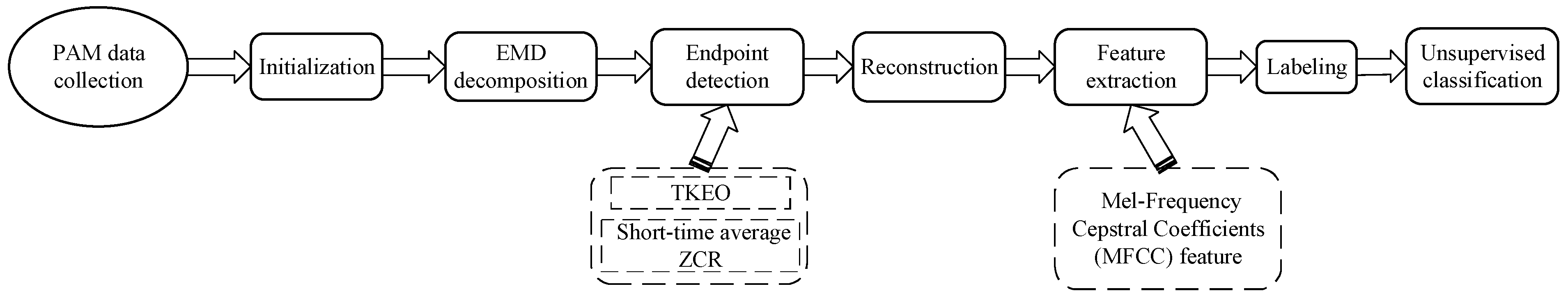
1.2. Automatic Detection

The automatic detection process contains two steps: endpoint detection and reconstruction. Firstly, all the WAVE files are read into digital format by MATLAB function “audioread”, and the Hamming window frames each sound to exclude some long-duration sounds. Then, a dual parameters–dual thresholds endpoint detection method based on EMD (empirical mode decomposition) [32] is conducted to detect the frequency variation within the sounds. Finally, the potential vocal signals are extracted and reunited to create a new acoustic signal. Consequently, background noise is removed from the audio files, and only the vocal signals are left in the new acoustic signal [33].

The methodology details of the EMD-based endpoint detection method for cetacean vocal signals are presented in Appendix A. We introduce the processes briefly in this section. Before detection, the collected waveform is initialized by eliminating the DC (direct current) components and normalizing the amplitudes. Firstly, the PAM data are transformed into EMD signals. Then, two adaptive thresholds are computed for automatic detection. Finally, the vocal signals are extracted from PAM data, and the clutters are removed. This method grabs the acoustic features of vocal signals and distinguishes them from the background clutters of the ocean environment. Two parameters—TKEO and short-time average ZCR (Zero crossing rate)—are computed and set as thresholds based on the IMF (intrinsic mode function) components. The average TKEO energy for each IMF component is calculated according to the frame size, and the frame length is set at 25 ms. These parameters are used to determine the front end and back end of vocal signals as well as filter out the background clutters without any prior information. We not only detect the endpoints of vocal signals but also extract the signals between the front end and back end points. The application of the TKEO on an underwater acoustic signal containing all IMF components reflects the energy distribution of the transient signal and produces an output for endpoint detection. More details of the endpoint detection method can be found in [32].

1.3. Feature Extraction

Feature extraction transforms vocal signals into a set of feature vectors that represent the distinct characteristics of the vocal signals. The new acoustic signals from the previous section are transformed into MFCC (mel-frequency cepstral coefficients) features. After receiving the feature vector, the label information is saved to verify the unsupervised classification. However, the duration of different vocal signals is not the same, which makes it difficult to build a formal feature vector. Our method is to use a Hamming window to enframe the signal and specify the window length as one frame per row. The length of a segment depends on the window length, while the frame size refers to the beginning position of the next segment. Here, a 75% overlapped Hamming window with length $M=2000$ is used by periodic sampling.

Furthermore, to improve the quality of the feature vector, each frame of the signal filtered by the Hamming window is transformed into an MFCC feature. It generates the coefficients corresponding to each data window for the input audio signal and converts the signal to a frequency representation at a certain sampling rate. The “audioread” function is used to read the audio file and get the sampling rate. The sampling rate here depends on the characteristics of the original cetacean vocal signal. The processes of the MFCC method include the following: 1. Framing; 2. Fast Fourier transform; 3. Calculate the periodogram estimate of the power spectrum; 4. Sum the energy passing through the mel filterbank; 5. Take the logarithm of all filterbank energies and the DCT of the log filterbank energies; 6. Obtain the MFCC coefficients. More detailed descriptions of the MFCC method are available at [34].

We only process the underwater acoustic data of the same cetacean species at a time and obtain its feature vector. Meanwhile, the corresponding label information is saved for later verification experiments. The vocal features of the same species are attached to the same label number and arranged into a column vector. After reviewing all the audio files, all species’ features are grouped into different combinations to create two to five classification datasets. Afterward, the unsupervised clustering-based classification is conducted on these mixture feature vectors. Eight datasets were formulated according to our methods. Overall, we analyze five cetacean species’ acoustic data during the detection process and count the file size before and after detection to sum up the extraction rate. Since the number and the size of each audio file are not the same, it is difficult to calculate the statistical extraction rate based on the time information, so the total size of the audio files are calculated. We also analyze the features of different species with mean value and standard deviation in

Table 1. Feature information.

Class Name	Species	Sample Number	Mean Values	Standard Deviation
RD	Rissos’ Dolphin	1799	$6.45\times {10}^{-6}$	$2.75\times {10}^{-10}$
RW	Right Whale	2257	$7.98\times {10}^{-5}$	$2\times {10}^{-8}$
PW	Pilot Whale	264	$2.31\times {10}^{-6}$	$1.11\times {10}^{-11}$
BW	Beaked Whale	722	$1.97\times {10}^{-5}$	$2.04\times {10}^{-9}$
CD	Common Dolphin	184	$2.02\times {10}^{-5}$	$6.98\times {10}^{-9}$
NW	Environmental Sound	8985	$1.2\times {10}^{-2}$	$9.89\times {10}^{-5}$

.

1.4. Unsupervised Classification

We use the vocal features picked out from the automatic detection process for unsupervised clustering-based classification and implement the categorization of multiple cetacean species. Conventional clustering algorithms such as K-means, PCA (principal component analysis), GMM, and SSC (sparse subspace clustering) are conducted for comparison. We demonstrate that different clustering methods show distinct clustering ability for classifying vocal signals. Four typical clustering algorithms are evaluated as unsupervised classification of five cetacean species. Clustering is a method to classify the data into different clusters by analyzing the intrinsic relationship between the data. The data points in the same cluster have similar characteristics and stick closer than those in different clusters. The classic types of clustering algorithms include the distance-based method such as K-means [35], dimension reduction clustering such as PCA [36], subspace clustering such as SSC [37], probabilistic models such as GMM [38], etc. To test the availability of the datasets, the clustering algorithms are performed on the datasets. In the meantime, we are interested in measuring the classification performance of different clustering algorithms on the datasets. Consequently, the four types of clustering algorithms, including K-means, PCA, SSC, and GMM, are applied for comparison.

K-means has been used to cluster time series data, achieving efficient clustering results due to its high speed, simplicity, and ease of implementation [39]. The K-means algorithm assigns the samples into K clusters by calculating and comparing the Euclidean distance between data points iteratively. The K in the algorithm is the class number of cetacean species within a dataset. PCA is a dimension reduction method that maps high-dimensional time-series data into low-dimensional features by orthogonal decomposition and then clusters the new orthogonal features, also known as the principal components. In other words, PCA eliminates the clutter signals in the data and preserves the most significant information; thus, the principal feature can be effectively extracted from time-series data [40]. GMM has shown improved classification for underwater bioacoustic data such as fish chorusing events [29,41,42], odontocetes’ vocal signals [18,19,43]. GMM is a probabilistic model that estimates the probabilities of data points in each cluster and categorizes them into the same cluster according to their probability. The probabilistic of a class represents the distribution of these class subsets within the whole dataset. Therefore, GMM can be applied not only in supervised classification but also in unsupervised classification. SSC aims to reveal the essential characteristics of data and use the sparsity of data in a specific space to represent data. It has been successfully and widely applied in many fields such as image processing [44,45,46,47], pattern recognition [48,49,50], and subspace clustering of high dimensional data [37,51,52]. SSC is based on the assumption that similar data will be in the same subspace structure, aiming at building a learning model for the dataset to learn a self-representation matrix and then using basic clustering algorithms such as spectral clustering and K-means to partition the self-representation matrix. Comparing the classification performance of these four types of clustering methods on our datasets will not only help to test the availability of our datasets but also verify the clustering ability of these algorithms on vocal features.

1.5. Evaluation Metrics

The performance of the clustering methods is evaluated by two metrics: average clustering accuracy (ACC) and F-score [53]. The statistical analysis of data and the evaluation metrics of unsupervised clustering methods are shown in the next section. The ground truth labels saved in the feature extraction are compared with those predicted by the clustering. The ACC is the proportion of correctly classified samples to the total number of samples. The format of ACC ($A_c$) is defined as follows:

$$\begin{array}{cc}\hfill A_c& ={\displaystyle \frac{1}{N}}\sum _{k=1}^N\mathbb{F}[I\left(k\right),H\left(k\right)],\hfill \\ \hfill \mathbb{F}\left[I\right(k),H(k\left)\right]& =\left\{\begin{array}{cc}1,\hfill & I\left(k\right)=H\left(k\right),\hfill \\ 0,\hfill & I\left(k\right)\ne H\left(k\right),\hfill \end{array}\right.\hfill \end{array}$$

(1)

where N is the total number of samples. k is the index of sample labels. $I\left(k\right)$ is the ground truth labels corresponding to different cetaceans saved in the feature extraction. $H\left(k\right)$ is the prediction label corresponding to different cetaceans predicted by the clustering. $\mathbb{F}[·]$ is the indicator function to compare the labels. $I\left(k\right)=H\left(k\right)$ means the ground truth label is correctly predicted. $\mathbb{F}\left[I\right(k),H(k\left)\right]=1$ means the classification of this specie’s vocal feature is successful, otherwise $\mathbb{F}\left[I\right(k),H(k\left)\right]=0$.

The F-score is another form of accuracy measurement on a classification dataset. It combines the precision and recall of the model to calculate the harmonic mean. Precision (also called positive predictive value) measures the ratio of correctly identified cetacean species to the total predicted species number. Recall (also called true positive rate) measures the ratio of correctly identified cetacean species to the total true species number. The definition of F-score ($F_s$) is given as follows:

$$\begin{array}{cc}\hfill Precision& ={\displaystyle \frac{TP}{PP}},Recall={\displaystyle \frac{TP}{P}},\hfill \\ \hfill F_s& =2\times {\displaystyle \frac{precision\times recall}{precision+recall}},\hfill \end{array}$$

(2)

where $TP$ refers to the total number of correctly classified cetacean species. In other words, it is the number of each cetacean species correctly grouped into their same species. $PP$ is the number of positive predictive, which is predictions for each cetacean species. P is the number of true cetacean species. The values of ACC and F-score are between 0 and 1. The higher the ACC and F-score rates, the better the classification performance.

2. Experiments and Results

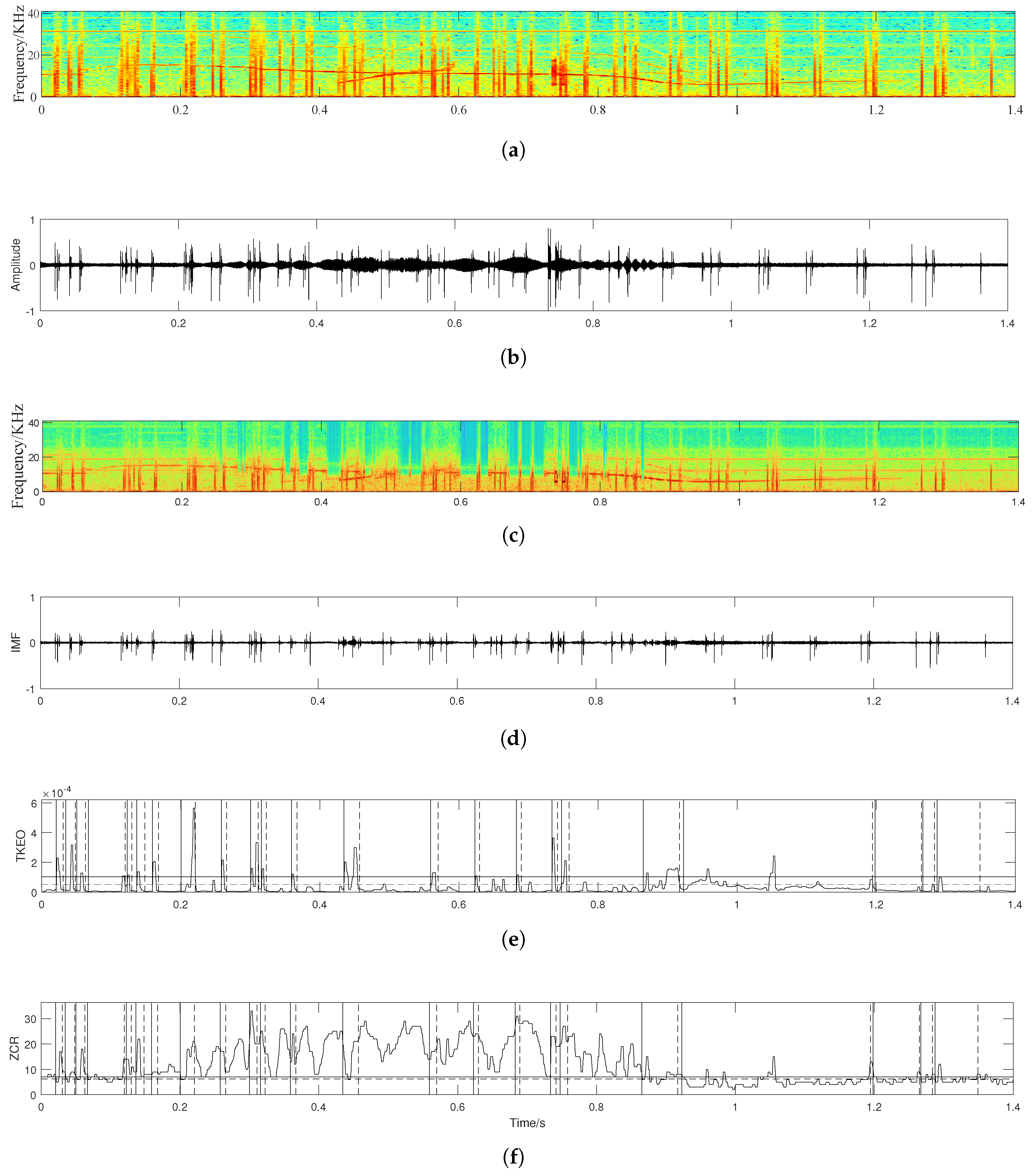
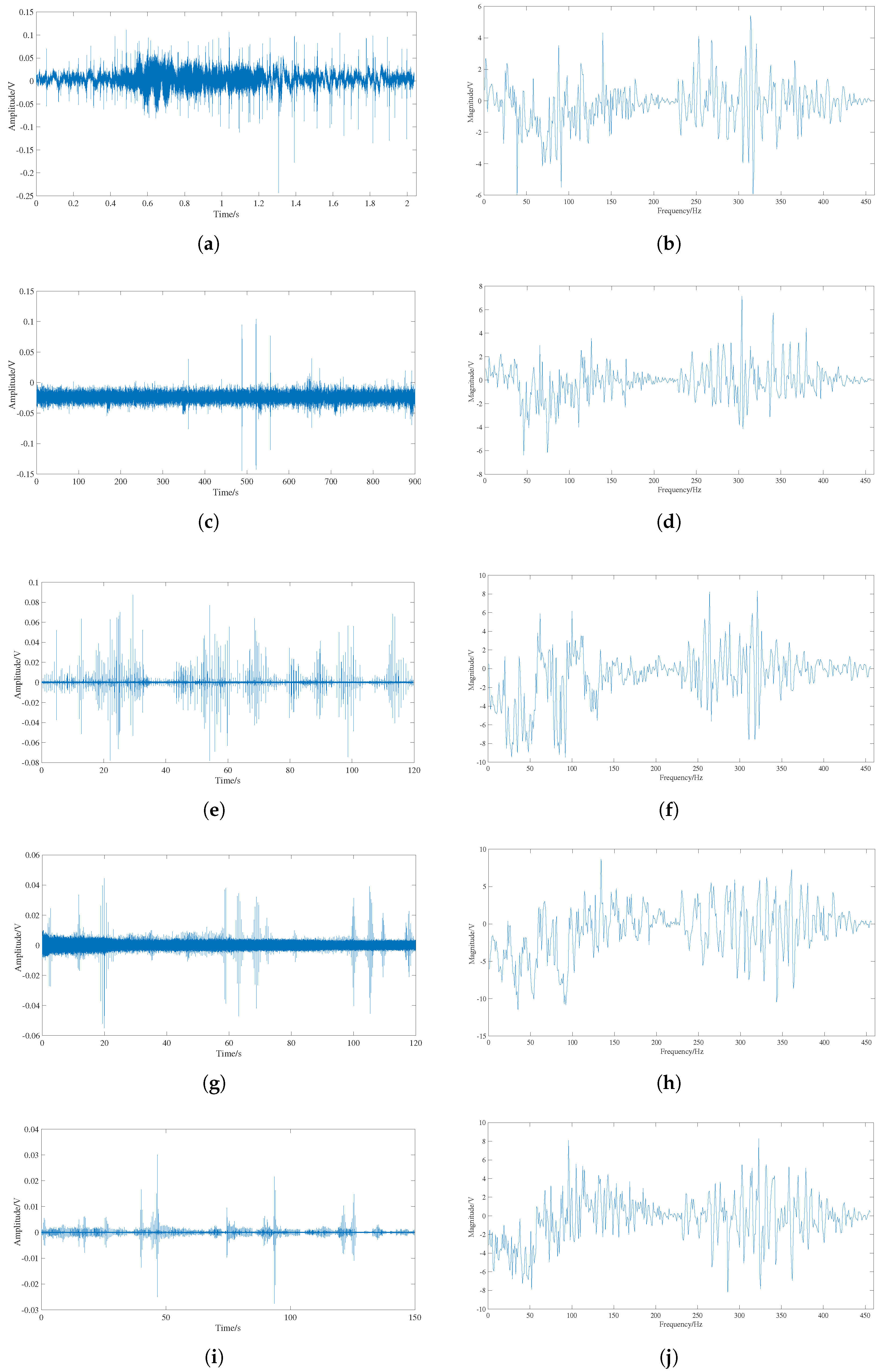
2.1. Detection

A total of 194 audio files have been analyzed by the proposed automatic detection method. An initialized signal waveform of the common dolphin is shown in Figure 2b, and the corresponding time-frequency spectrogram is displayed in Figure 2a. The settings of this spectrogram are 81.6 KHz sampling rate, 50% overlap, and a total of 256 frequency points used to calculate the discrete Fourier transforms. Then, the dual parameters–dual thresholds endpoint detection method is employed for the acoustic signals after initialization. There are three transformations in endpoint detection. Firstly, EMD is used to reconstitute the initialized audio signals into IMF components to reveal the intrinsic mode of the vocal signals.

The audio signal spectrogram and waveform reconstructed by EMD are shown in Figure 2c. Secondly, the average TKEO energy for each IMF component is calculated according to the frame size, and the frame length is set at 25 ms. The IMF components are transformed into the TKEO shown in Figure 2d. The horizontal solid and the dashed line are two grade thresholds computed by the mean value of TKEO or ZCR for each frame but in different sizes. The first grade threshold solid line is used for rough estimation and set higher than the second threshold. The second grade threshold dashed line is slightly lower than the threshold for more accurate estimation. For example, the value of the first grade threshold in Figure 2d is set as $3\times TE$, and the value of the second grade threshold is set as $1.5\times TE$. The numbers 3 and 1.5 are multiples of the thresholds, and they are also the empirical value set according to the experiment. The lines in Figure 2e are plotted in the same way. The value of the first grade threshold in Figure 2e is set as $0.9\times ZCR$ and the value of the second grade threshold is set as $0.8\times ZCR$. The variables $ZCR$ and $TE$ have been defined in Appendix A. Finally, another parameter threshold, short-time average ZCR, is measured frame by frame from the initialized audio signals shown in Figure 2e. After the energy transformation, the energy amplitude at each moment is compared with the average TKEO and short-time average ZCR of the signals. When the value exceeds two grade thresholds of two parameters, it is considered as the beginning of the vocal call. Two-level decisions are judged for whether they are in a vocal segment. The start points are recorded in vertical solid lines, and the endpoints are recorded in vertical dashed lines. The segments between the start and endpoints are the potential vocal signals. We compare the different forms of the acoustic signals of CD and show the picked vocal signals in Figure 2.

In the experiment discussed above, we assume that the spectrograms are free from distortion. However, in oceanic environments, the PAM signal may experience frequency drift due to the Doppler effect, which results from the relative movement between cetaceans and the monitoring sensors. Detecting and compensating for this frequency drift is a challenging task. Fortunately, researchers have developed effective solutions. A recent advanced method by G. Avon et al. utilized a straightforward yet efficient lookup-table approach based on multi-jump resonance systems, mapping the frequency drift to an amplitude jump [54,55]. In this paper, signals are sourced from open-access databases, but the available information regarding monitoring sensors and the environment is limited. Therefore, the direct application of existing schemes, if feasible, is not straightforward. For this reason, we will temporarily overlook the frequency drift and address it in future work.

We also compare our detection method with the Teager–Kaiser energy operator detection method in [9] in Figure 3b. A cut of the collected waveform of the common dolphin, also used in Figure 2, is chosen and captured in the 0.1 s fragment for comparison. In Figure 3, two detection methods are performed on the same waveform period, and the signals between the solid lines and the dashed lines are the vocal signals detected. The detection of common dolphin vocal signals based on the dual parameters–dual thresholds endpoint detection method is shown in Figure 3a. Figure 3b shows the detection of common dolphin vocal signals based on the TKEO detection method [9] for comparison. Figure 3 is the amplification version of the waveform before 0.1 s, which is used to confirm the scope of the vocal signals and compare the effectiveness of the two detection methods. All the segments are saved for reconstruction, and the background noises are removed from the sections of audio signals. The segments of vocal signals are the output of the TKEO. Since only the vocal signal is needed for the feature vector, the most obvious peak characteristic of the vocal signals are picked out and combined to observe the peak value variation. Finally, the mel frequency cepstral coefficients (MFCCs) of the reconstruction signals are computed using the MFCC function. In Figure 4, the waveform of the original acoustic signals is shown on the left side of the figure, and the MFCC feature of the reconstruction signals on the right side of the figure.

The classification datasets comprise these five cetacean species’ acoustic and environmental data. The details of these datasets are listed in

Table 2. The information of the datasets for two to five classifications.

	Dataset	Class	Sample	Species
1	RDRW	2	3598	Rissos’ Dolphin, Right Whale
2	RWNW	2	4514	Right Whale, NoWhale *
3	RDNW	2	3598	Rissos’ Dolphin, NoWhale
4	RDPWBW	3	792	Rissos’ Dolphin, Pilot Whale, Beaked Whale
5	CDRWNW	3	552	Common Dolphin, Right Whale, NoWhale
6	RDRWNW	3	5397	Rissos’ Dolphin, Right Whale, NoWhale
7	RWRDPWBW	4	1056	Rissos’ Dolphin, Right Whale, Pilot Whale, Beaked Whale
8	NWRWRDPWBW	5	1320	NoWhale, Right Whale, Rissos’ Dolphin, Pilot Whale, Beaked Whale

* This is the environmental sound without whale calls.

, and to be simplified, the abbreviation of datasets are named according to the acronym of cetacean species. The statistics information of different cetacean species’ acoustic data is summarized in

Table 3. The statistics of cetaceans’ audio files. Reproduced with permission from Liang, Y. et al., published by IEEE International Conference on Electrical, Automation and Computer Engineering (ICEACE), 2023 [33].

Cetacean Species (Abbreviation)	File Number (n)	Before (MB)	After (MB)	Extraction Rate (%)
Common Dolphin (CD)	61	42.3	2.61	6.17
Right Whale (RW)	96	329	33	10.03
Risso’s Dolphin (RD)	13	452	26	5.75
Pilot Whale (PW)	8	263	3.74	1.42
Beaked Whale (BW)	16	495	10.4	2.1
Total	194	1581.3	75.75	25.47

.

2.2. Clustering

After automatic detection and feature extraction, the potential vocal signals detected by our algorithm are combined together and transformed into the MFCC feature for classification. The datasets are built with these MFCC features of different cetacean species. To verify the feature vector, unsupervised classification methods are performed on the datasets listed in Table 2. Various vocal signals are randomly selected and combined for clustering. The two classification datasets contain two class combinations such as the Rissos’ dolphin and right whale (RDRW) combination, right whale and no whale (RWNW) combination, Rissos’ dolphin and no whale (RDNW) combination. Similarly, the three classification datasets are made of three class combinations, the same as the four and five classification datasets. Afterward, four clustering algorithms (K-means, PCA, GMM, SSC) are evaluated on these datasets using two metrics (ACC and F-score) mentioned above. The clustering accuracy of each dataset is ranged from 0 to 100%. We run each clustering algorithm ten times and record the mean square error according to the ten-time results. The clustering results via ACC and F-score metric on different datasets are listed in

Table 4. Clustering results of the datasets evaluated by ACC metric (%).

Class Number	Dataset	K-Means	PCA	GMM	SSC
m = 2	RDRW	$94.44\pm 0.41$	91.20 ± 0.59	92.86 ± 0.11	73.84 ± 0.66
	RWNW	99.69 ± 0.23	99.72 ± 0.15	$99.80\pm 0.01$	98.18 ± 0.1
	RDNW	99.86 ± 0.1	99.63 ± 0.45	$100.00\pm 0$	97.76 ± 0.65
m = 3	RDPWBW	$75.70\pm 0.32$	74.01 ± 0.51	74.47 ± 0.05	58.48 ± 0.53
	CDRWNW	92.46 ± 0.24	92.78 ± 0.25	$92.83\pm 0.49$	87.32 ± 0.88
	RDRWNW	$96.10\pm 0.12$	95.78 ± 1.56	94.51 ± 0.01	86.49 ± 0.25
m = 4	RWRDPWBW	$75.52\pm 0.42$	72.51 ± 0.83	69.07 ± 1.40	40.80 ± 0.29
m = 5	NWRWRDPWBW	$80.28\pm 0.27$	78 ± 1.19	76.23 ± 0.58	54.19 ± 0.64

and

Table 5. Clustering results of the datasets evaluated by F-score metric (%).

Class Number	Dataset	K-Means	PCA	GMM	SSC
m = 2	RDRW	$89.49\pm 0.48$	84.08 ± 0.95	77.92 ± 1.12	64.00 ± 0.82
	RWNW	99.38 ± 0.14	99.45 ± 0.29	$99.47\pm 0.00$	96.42 ± 0.68
	RDNW	99.72 ± 0.16	99.26 ± 0.90	$100.00\pm 0.00$	95.59 ± 0.52
m = 3	RDPWBW	$66.18\pm 0.56$	62.58 ± 0.82	63.34 ± 0.09	44.235 ± 0.41
	CDRWNW	86.78 ± 0.35	87.27 ± 0.38	$87.31\pm 0.74$	77.76 ± 0.58
	RDRWNW	$92.63\pm 0.24$	92.06 ± 2.68	89.86 ± 0.02	77.22 ± 0.23
m = 4	RWRDPWBW	$62.35\pm 0.61$	57.39 ± 0.99	52.95 ± 1.94	31.25 ± 0.16
m = 5	NWRWRDPWBW	$69.32\pm 0.47$	65.58 ± 1.35	62.80 ± 0.61	44.55 ± 0.15

.

3. Discussion

An automatic processing method is proposed to extract the vocal features of five cetacean species from two open source databases and reconstruct the vocal features to build the eight datasets. Then, the clustering algorithm is used to achieve the unsupervised classification and verify the effectiveness of the datasets for classification. The results will be discussed in two dimensions: detection and clustering results.

In the detection results, each step of endpoint detection is put together to compare the graphical changes and show the different forms of the acoustic signals in Figure 2. In the beginning, the collected waveform of the common dolphin after initialization still has significant noise, and some vocal signals are covered by noise. As shown in Figure 2c, the EMD method helps to eliminate the background noise and reveals most of the vocal signals. TKEO reflects the energy variation of the audio signal after EMD and traces the characteristics of a section signal. It strengthens the vocal parts and attenuates the unstable noise parts. The collected waveform is simplified into a curve representing the energy variation. The short-time average ZCR curve is shown in the same way. Most vocal signals in this figure are detected and recognized.

The comparison of the two detection methods in Figure 3 shows that our method finds more information on the vocal signals than the TKEO detection method. This is because our detection method locates the vocal signals according to the endpoints, while the TKEO detection method locates the vocal signals at the peaks and the single threshold. Through the enlarged image of 0.1 s signal in Figure 3, it’s observed that the endpoint detection method selects the vocal signals from the front end of high peaks to the back end of the lower peaks. However, the TKEO detection method may not contain all the whole vocal signals due to the limitation of the threshold-based technique.

A visual comparison between the collected waveform and the reconstruction signals is shown in Figure 4. In the beginning, the collected waveform is full of noise, and it is difficult to distinguish between the background noise and the vocal signals. The proposed detection method cuts off the background noise and reserves the stronger and clearer parts of the vocal signals to observe the energy changes of the vocal signals. For example, the effectiveness of endpoint detection is shown in Figure 2 and Figure 3. The vocal signal is simplified into a single MFCC curve. In this way, the vocal signals are better revealed concisely and clearly.

Moreover, the extraction rates from the statistics Table 3 do not exceed 10% or just around 10%. It indicates that the vocal signals within a section of the acoustic signals are rare. If the whole audio file is taken as the classification feature, it will be difficult to train for classification. Thus, it is a good choice to select the most significant parts of the vocal signals to build the feature vectors and concentrate all the vocal signals to analyze them conveniently. The acoustic data of some cetacean species in the database are rare and insufficient for classification training, and the deep learning method may not be suitable here. The unsupervised clustering methods do not need too much data for pretraining and classifying data according to their internal characteristics. In this paper, the unsupervised clustering-based classification method performs well on feature vectors.

The clustering results in Table 4 and Table 5 demonstrate the classification accuracy of different clustering methods on our datasets. With the increasing number of species classes, it becomes harder to classify the different vocal signals of cetaceans, and the clustering accuracy decreases. Classical unsupervised clustering algorithms obtain an average accuracy rate of 84.83%. However, the ACC results of the five-class dataset can be up to 80%. From the comparison of clustering methods, K-means and GMM perform better than the PCA and SSC in classifying our datasets. The clustering results evaluated by the F-score metric are lower than the ACC results, but the tendency of the results is alike. Nevertheless, the proposed method has a higher classification accuracy than the GMM and SVM methods in [18,19], with 67-75% accuracy in classifying three species. The DEC method in [29] achieves the highest accuracy of 77.5% to classify two distinguishing signals (the vocal and coral reef bioacoustic signals) in the manually labeled dataset. Our method classifies five classes of species with high accuracy. Generally, K-means and GMM are more capable of classifying the vocal signals than the other two methods. However, K-means is more scalable than GMM because K-means performs well not only on small-class datasets but also in larger-class datasets. However, the accuracy of GMM is decreasing with the increasing number of classes.

4. Conclusions

The proposed method has achieved automatic detection and unsupervised clustering-based classification on our datasets. The proposed method extracts the vocal features from the collected waveform in a total of 25.3 h of vocal signals and combines the five cetacean species’ vocal signals to build eight classes of datasets for classification. Then, the performances of different clustering methods on our datasets are verified. As a result, K-means and GMM perform well on our datasets. The maximum accuracy rate is 100% for the GMM method. When using the K-means algorithm, the accuracy rate achieved can be as low as 75%. In this work, the proposed method is completely non-manual operation and reduces time costs. The feature vectors have broad applicability and can be used to test other automatic classification methods. Our method inspires future work to detect and classify acoustic signals from cetaceans automatically. However, this method still cannot accurately classify all cetaceans when there are multiple classes. There is still much work to pursue in the future. On one hand, the detection methods should recognize the vocal signals more accurately. On the other hand, when more cetacean species are shown simultaneously, the accuracy of classification needs to be improved. The proposed method is more suitable for pre-processing in acoustic data processing since it is easy to distinguish the vocal signals and the background noise.

References

1. Braulik, G.T.; Taylor, B.L.; Minton, G.; Notarbartolo di Sciara, G.; Collins, T.; Rojas-Bracho, L.; Crespo, E.A.; Ponnampalam, L.S.; Double, M.C.; Reeves, R.R. Red-list status and extinction risk of the world’s whales, dolphins, and porpoises. Conserv. Biol. 2023, 37, e14090. [Google Scholar]
2. Mellinger, D.K.; Stafford, K.M.; Moore, S.E.; Dziak, R.P.; Matsumoto, H. An Overview of Fixed Passive Acoustic Observation Methods for Cetaceans. Oceanography 2007, 20, 36–45. [Google Scholar]
3. Zimmer, W.M. Passive Acoustic Monitoring of Cetaceans; Cambridge University Press: Cambridge, UK, 2011. [Google Scholar]
4. Rankin, S.; Archer, F.; Keating, J.L.; Oswald, J.N.; Oswald, M.; Curtis, A.; Barlow, J. Acoustic classification of dolphins in the California Current using whistles, echolocation clicks, and burst pulses. Mar. Mammal Sci. 2017, 33, 520–540. [Google Scholar]
5. Griffiths, E.T.; Archer, F.; Rankin, S.; Keating, J.L.; Keen, E.; Barlow, J.; Moore, J.E. Detection and classification of narrow-band high frequency echolocation clicks from drifting recorders. J. Acoust. Soc. Am. 2020, 147, 3511–3522. [Google Scholar]
6. Staaterman, E. Passive Acoustic Monitoring in Benthic Marine Crustaceans: A New Research Frontier. In Listening in the Ocean; Au, W.W.L., Lammers, M.O., Eds.; Springer: New York, NY, USA, 2016; pp. 325–333. [Google Scholar]
7. Wiggins, S.M.; Hildebrand, J.A. High-frequency Acoustic Recording Package (HARP) for broad-band, long-term marine mammal monitoring. In Proceedings of the 2007 Symposium on Underwater Technology and Workshop on Scientific Use of Submarine Cables and Related Technologies, Tokyo, Japan, 17–20 April 2007; pp. 551–557. [Google Scholar]
8. Gillespie, D. An acoustic survey for sperm whales in the Southern Ocean Sanctuary conducted from the RSV Aurora Australis. Rep. Int. Whal. Comm. 1997, 47, 897–907. [Google Scholar]
9. Kandia, V.; Stylianou, Y. Detection of sperm whale clicks based on the Teager–Kaiser energy operator. Appl. Acoust. 2006, 67, 1144–1163. [Google Scholar]
10. Houser, D.S.; Helweg, D.A.; Moore, P.W. Classification of dolphin echolocation clicks by energy and frequency distributions. J. Acoust. Soc. Am. 1999, 106, 1579–1585. [Google Scholar]
11. Klinck, H.; Mellinger, D. The energy ratio mapping algorithm: A tool to improve the energy-based detection of odontocete echolocation clicks. J. Acoust. Soc. Am. 2011, 129, 1807–1812. [Google Scholar]
12. Gong, W.; Tian, J.; Liu, J.; Li, B. Underwater Object Classification in SAS Images Based on a Deformable Residual Network and Transfer Learning. Appl. Sci. 2023, 13, 899. [Google Scholar] [CrossRef]
13. Ji, F.; Li, G.; Lu, S.; Ni, J. Research on a Feature Enhancement Extraction Method for Underwater Targets Based on Deep Autoencoder Networks. Appl. Sci. 2024, 14, 1341. [Google Scholar] [CrossRef]
14. Krizhevsky, A.; Sutskever, I.; Hinton, G.E. ImageNet classification with deep convolutional neural networks. Commun. ACM 2017, 60, 84–90. [Google Scholar]
15. Luo, W.; Yang, W.; Zhang, Y. Convolutional neural network for detecting odontocete echolocation clicks. J. Acoust. Soc. Am. 2019, 145, EL7–EL12. [Google Scholar] [PubMed]
16. Yang, W.; Luo, W.; Zhang, Y. Classification of odontocete echolocation clicks using convolutional neural network. J. Acoust. Soc. Am. 2020, 147, 49–55. [Google Scholar] [PubMed]
17. Rasmussen, J.H.; Širović, A. Automatic detection and classification of baleen whale social calls using convolutional neural networks. J. Acoust. Soc. Am. 2021, 149, 3635–3644. [Google Scholar]
18. Roch, M.A.; Soldevilla, M.S.; Burtenshaw, J.C.; Henderson, E.E.; Hildebrand, J.A. Gaussian mixture model classification of odontocetes in the Southern California Bight and the Gulf of California. J. Acoust. Soc. Am. 2007, 121, 1737–1748. [Google Scholar]
19. Roch, M.; Soldevilla, M.; Hoenigman, R.; Wiggins, S.; Hildebrand, J. Comparison of Machine Learning Techniques for the Classification of Echolocation Clicks from Three Species of Odontocetes. Can. Acoust. 2008, 36, 41–47. [Google Scholar]
20. Luo, W.; Yang, W.; Song, Z.; Zhang, Y. Automatic species recognition using echolocation clicks from odontocetes. In Proceedings of the 2017 IEEE International Conference on Signal Processing, Communications and Computing (ICSPCC), Xiamen, China, 22–25 October 2017; pp. 1–5. [Google Scholar]
21. Roch, M.A.; Lindeneau, S.; Aurora, G.S.; Frasier, K.E.; Hildebrand, J.A.; Glotin, H.; Baumann-Pickering, S. Using context to train time-domain echolocation click detectors. J. Acoust. Soc. Am. 2021, 149, 3301–3310. [Google Scholar]
22. Jiang, J.J.; Bu, L.R.; Wang, X.Q.; Li, C.Y.; Sun, Z.B.; Yan, H.; Hua, B.; Duan, F.J.; Yang, J. Clicks classification of sperm whale and long-finned pilot whale based on continuous wavelet transform and artificial neural network. Appl. Acoust. 2018, 141, 26–34. [Google Scholar]
23. Trinh, Y.; Lindeneau, S.; Ackerman, M.; Baumann-Pickering, S.; Roch, M. Unsupervised clustering of toothed whale species from echolocation clicks. J. Acoust. Soc. Am. 2016, 140, 3302. [Google Scholar]
24. Frasier, K.E.; Elizabeth Henderson, E.; Bassett, H.R.; Roch, M.A. Automated identification and clustering of subunits within delphinid vocalizations. Mar. Mammal Sci. 2016, 32, 911–930. [Google Scholar]
25. Reyes Reyes, M.V.; Iñíguez, M.A.; Hevia, M.; Hildebrand, J.A.; Melcón, M.L. Description and clustering of echolocation signals of Commerson’s dolphins (Cephalorhynchus commersonii) in Bahía San Julián, Argentina. J. Acoust. Soc. Am. 2015, 138, 2046–2053. [Google Scholar]
26. Li, K.; Sidorovskaia, N.A.; Tiemann, C.O. Model-based unsupervised clustering for distinguishing Cuvier’s and Gervais’ beaked whales in acoustic data. Ecol. Inform. 2020, 58, 101094. [Google Scholar]
27. LeBien, J.G.; Ioup, J.W. Species-level classification of beaked whale echolocation signals detected in the northern Gulf of Mexico. J. Acoust. Soc. Am. 2018, 144, 387–396. [Google Scholar] [PubMed]
28. Frasier, K.E.; Roch, M.A.; Soldevilla, M.S.; Wiggins, S.M.; Garrison, L.P.; Hildebrand, J.A. Automated classification of dolphin echolocation click types from the Gulf of Mexico. PLoS Comput. Biol. 2017, 13, e1005823. [Google Scholar]
29. Ozanich, E.; Thode, A.; Gerstoft, P.; Freeman, L.A.; Freeman, S. Deep embedded clustering of coral reef bioacoustics. J. Acoust. Soc. Am. 2021, 149, 2587–2601. [Google Scholar]
30. Mellinger, D.K.; Clark, C.W. MobySound: A reference archive for studying automatic recognition of marine mammal sounds. Appl. Acoust. 2006, 67, 1226–1242. [Google Scholar]
31. Watkins, W.A.; Fristrup, K.; Daher, M.A.; Howald, T.J. Sound Database of Marine Animal Vocalizations Structure and Operations; Woods Hole Oceanographic Institution: Falmouth, MA, USA, 1992. [Google Scholar]
32. Li, M.M.; Yang, H.W.; Hong, N.; Yang, S. Endpoint detection based on EMD in noisy environment. In Proceedings of the 2011 6th International Conference on Computer Sciences and Convergence Information Technology (ICCIT), Seogwipo, Republic of Korea, 29 November–1 December 2011; pp. 783–787. [Google Scholar]
33. Liang, Y.; Chen, F.; Yu, H.; Chen, Y.; Ji, F. An EMD Based Automatic Endpoint Detection Method for Cetacean Vocal Signals. In Proceedings of the 2023 IEEE International Conference on Electrical, Automation and Computer Engineering (ICEACE), Changchun, China, 26–28 December 2023. [Google Scholar]
34. Rabiner, L.; Schafer, R. Theory and Applications of Digital Speech Processing; Prentice Hall Press: Saddle River, NJ, USA, 2010; pp. 1–1056. [Google Scholar]
35. Arthur, D.; Vassilvitskii, S. k-Means++: The Advantages of Careful Seeding; Technical Report 2006-13; Stanford InfoLab: San Francisco, CA, USA, 2006. [Google Scholar]
36. Yang, J.; Zhang, D.; Frangi, A.F.; Yang, J.Y. Two-dimensional PCA: A new approach to appearance-based face representation and recognition. IEEE Trans. Pattern Anal. Mach. Intell. 2004, 26, 131–137. [Google Scholar]
37. Elhamifar, E.; Vidal, R. Sparse subspace clustering: Algorithm, theory, and applications. IEEE Trans. Pattern Anal. Mach. Intell. 2013, 35, 2765–2781. [Google Scholar]
38. Liu, J.; Cai, D.; He, X. Gaussian mixture model with local consistency. In Proceedings of the AAAI Conference on Artificial Intelligence, Atlanta, GA, USA, 11–15 July 2010; Volume 24, pp. 512–517. [Google Scholar]
39. Ali, M.; Alqahtani, A.; Jones, M.W.; Xie, X. Clustering and classification for time series data in visual analytics: A survey. IEEE Access 2019, 7, 181314–181338. [Google Scholar]
40. Yang, K.; Shahabi, C. A PCA-based similarity measure for multivariate time series. In Proceedings of the 2nd ACM International Workshop on Multimedia Databases, Washington, DC, USA, 13 November 2004; pp. 65–74. [Google Scholar]
41. Lin, T.H.; Tsao, Y.; Akamatsu, T. Comparison of passive acoustic soniferous fish monitoring with supervised and unsupervised approaches. J. Acoust. Soc. Am. 2018, 143, EL278–EL284. [Google Scholar]
42. Brown, J.C.; Smaragdis, P. Hidden Markov and Gaussian mixture models for automatic call classification. J. Acoust. Soc. Am. 2009, 125, EL221–EL224. [Google Scholar] [CrossRef] [PubMed]
43. Peso Parada, P.; Cardenal-López, A. Using Gaussian mixture models to detect and classify dolphin whistles and pulses. J. Acoust. Soc. Am. 2014, 135, 3371–3380. [Google Scholar] [CrossRef] [PubMed]
44. Yang, J.; Wright, J.; Huang, T.S.; Ma, Y. Image super-resolution via sparse representation. IEEE Trans. Image Process. 2010, 19, 2861–2873. [Google Scholar] [PubMed]
45. Wu, C.; Zhao, J. Joint learning framework of superpixel generation and fuzzy sparse subspace clustering for color image segmentation. Signal Process. 2024, 222, 109515. [Google Scholar] [CrossRef]
46. Song, S.; Ren, D.; Jia, Z.; Shi, F. Adaptive Gaussian Regularization Constrained Sparse Subspace Clustering for Image Segmentation. In Proceedings of the ICASSP 2024—2024 IEEE International Conference on Acoustics, Speech and Signal Processing (ICASSP), Seoul, Republic of Korea, 14–19 April 2024; IEEE: New York, NY, USA, 2024; pp. 4400–4404. [Google Scholar]
47. Razik, J.; Glotin, H.; Hoeberechts, M.; Doh, Y.; Paris, S. Sparse coding for efficient bioacoustic data mining: Preliminary application to analysis of whale songs. In Proceedings of the 2015 IEEE International Conference on Data Mining Workshop (ICDMW), Atlantic City, NJ, USA, 14–17 November 2015; IEEE: New York, NY, USA, 2015; pp. 780–787. [Google Scholar]
48. Wright, J.; Ma, Y.; Mairal, J.; Sapiro, G.; Huang, T.S.; Yan, S. Sparse representation for computer vision and pattern recognition. Proc. IEEE 2010, 98, 1031–1044. [Google Scholar] [CrossRef]
49. Sui, Y.; Wang, G.; Zhang, L. Sparse subspace clustering via low-rank structure propagation. Pattern Recognit. 2019, 95, 261–271. [Google Scholar]
50. Goel, A.; Majumdar, A. Sparse subspace clustering incorporated deep convolutional transform learning for hyperspectral band selection. Earth Sci. Inform. 2024, 17, 2727–2735. [Google Scholar] [CrossRef]
51. Xing, Z.; Peng, J.; He, X.; Tian, M. Semi-supervised sparse subspace clustering with manifold regularization. Appl. Intell. 2024, 54, 6836–6845. [Google Scholar] [CrossRef]
52. Sui, J.; Liu, Z.; Liu, L.; Jung, A.; Li, X. Dynamic sparse subspace clustering for evolving high-dimensional data streams. IEEE Trans. Cybern. 2020, 52, 4173–4186. [Google Scholar] [CrossRef]
53. Powers, D.; Ailab. Evaluation: From precision, recall and F-measure to ROC, informedness, markedness and correlation. J. Mach. Learn. Technol. 2011, 2, 2229–3981. [Google Scholar]
54. Avon, G.; Bucolo, M.; Buscarino, A.; Fortuna, L. Sensing frequency drifts: A lookup table approach. IEEE Access 2022, 10, 96249–96259. [Google Scholar] [CrossRef]
55. Buscarino, A.; Famoso, C.; Fortuna, L.; Frasca, M. Multi-jump resonance systems. Int. J. Control 2020, 93, 282–292. [Google Scholar] [CrossRef]
56. Mandic, D.P.; ur Rehman, N.; Wu, Z.; Huang, N.E. Empirical mode decomposition-based time-frequency analysis of multivariate signals: The power of adaptive data analysis. IEEE Signal Process. Mag. 2013, 30, 74–86. [Google Scholar] [CrossRef]
57. Kaiser, J. On a simple algorithm to calculate the ‘energy’ of a signal. In Proceedings of the International Conference on Acoustics, Speech, and Signal Processing, Albuquerque, NM, USA, 3–6 April 1990; Volume 1, pp. 381–384. [Google Scholar]
58. Junqua, J.C.; Reaves, B.; Mak, B. A study of endpoint detection algorithms in adverse conditions: Incidence on a DTW and HMM recognizer. In Proceedings of the Eurospeech, Genova, Italy, 24–26 September 1991; Volume 91, pp. 1371–1374. [Google Scholar]
59. Giannakopoulos, T.; Pikrakis, A. Introduction to Audio Analysis Chapter 4—Audio Features; Academic Press: Oxford, UK, 2014; pp. 59–103. [Google Scholar]
Figure 1. The workflow diagram for automatic detection and classification process.
Applsci 15 03585 g001
Figure 2. The result of dual parameters dual thresholds endpoint detection based on EMD. (a) The signal spectrogram of common dolphin after initialization. (b) The signal waveform of common dolphin after initialization. (c) The signal spectrogram of common dolphin after EMD decomposition. (d) The signal waveform of common dolphin after EMD decomposition. (e) The mean value of Teager-Kaiser energy operator. (f) Zero crossing rate of the signal. (The vertical solid lines represent the start points and the dashed lines represent the endpoints. The horizontal solid lines and the dashed lines are two-grade thresholds. Color indicates normalized log power (dB)). Reproduced with permission from Liang, Y. et al., published by IEEE International Conference on Electrical, Automation and Computer Engineering (ICEACE), 2023 [33].
Applsci 15 03585 g002
Figure 3. Comparison of different methods for detecting common dolphin vocal signals: (a) Detection of common dolphin vocal signals based on dual parameters-dual thresholds endpoint detection method. (b) Detection of common dolphin vocal signals based on the Teager-Kaiser energy operator method. (The black solid lines represent the start points, and the red dashed lines represent the endpoints). Reproduced with permission from Liang, Y. et al., published by IEEE International Conference on Electrical, Automation and Computer Engineering (ICEACE), 2023 [33].
Applsci 15 03585 g003
Figure 4. The figures on the left side are the collected waveform of cetacean vocalizations. The other side is the MFCC feature of the reconstruction signals. (a) The waveform of CD. (b) Reconstruction signal of CD. (c) The waveform of RW. (d) Reconstruction signal of RW. (e) The waveform of RD. (f) Reconstruction signal of RD. (g) The waveform of PW. (h) Reconstruction signal of PW. (i) The waveform of BW. (j) Reconstruction signal of BW.
Applsci 15 03585 g004