Research on Investment Estimation of Prefabricated Buildings Based on Genetic Algorithm Optimization Neural Network

Abstract

At present, China’s prefabricated buildings have entered a period of comprehensive development. Starting from the investment decision-making stage of construction projects, this paper analyses the characteristics of prefabricated investment estimation and the relevant literature on the characteristics of prefabricated construction projects, uses the rough set attribute reduction algorithm to screen the key engineering characteristic factors, and establishes a BP neural network model optimized by genetic algorithm to estimate and analyze the investment of completed prefabricated construction projects. The results of the study show that the accuracy of the improved BP neural network prediction model is better than that of the standard BP neural network prediction model, and the results are more stable, which provides a more scientific and effective method for the investment estimation of prefabricated buildings projects.

1. Introduction

Investment estimation is one of the important contents of the preliminary work of engineering construction, and is an important basis for the feasibility study and investment decision-making [1]. At this stage of China’s prefabricated buildings standardization, integration degree is insufficient, thus resulting in difficult to reduce the construction cost greatly restricts its benign development. In order to further promote the development of prefabricated construction projects and meet the reinvestment estimation needs of prefabricated construction projects, China’s Ministry of Housing and Urban–Rural Development issued the “Investment Estimation Indicators for Prefabricated Construction Projects” in 2023. Therefore, how to accurately control the investment estimation of prefabricated building projects is gradually becoming the focus of research on prefabricated building management. Due to the different production and construction methods between prefabricated buildings and traditional buildings, using traditional methods such as capital turnover rate method, production capacity index method, and comprehensive index investment estimation method to estimate prefabricated buildings is inevitably unreasonable, and digital technology must be introduced for fast and accurate estimation.

In the era of coordinated development of intelligent construction and building industrialization, the innovation and iteration speed of digital technology in China has significantly accelerated. Digital technology is also integrating into various fields of our lives with new concepts, new formats, and new models, and artificial intelligence is one of them. With the rise in artificial intelligence, machine learning models and deep learning techniques have gradually attracted the attention of scholars. As deep learning usually requires a large amount of data for training to fully utilize its advantages, this article selects machine learning for regression prediction of prefabricated building investment estimation. Meanwhile, considering the nonlinear relationship between the characteristic parameters and output indicators of the selected project in this study, a nonlinear model will be selected for prediction in this paper.

Nonlinear models in machine learning typically include methods such as XGBoost, decision trees, random forests, support vector machines, and neural networks. Among them, neural networks, as an important direction of artificial intelligence, have been introduced into the field of engineering investment estimation by many scholars. Based on previous research, this paper will use genetic algorithms to optimize the BP neural network method for investment estimation of prefabricated buildings, solving the limitations of decision tree instability, large memory consumption of random forests, and poor interpretability of support vector machines. At the same time, it enhances global search ability, avoids local optima, avoids overfitting, and improves model training efficiency. In the current era of machine learning, scholars have also begun to use this method to study investment estimation in the engineering field. In addition, scholars’ research on genetic algorithms is constantly deepening.

Yan, HY, and others proposed a prefabricated concrete building investment estimation model based on the XGBoost machine learning algorithm. The construction feature indicators of prefabricated building investment estimation were extracted using the construction project cost significance theory and the analytic hierarchy process. Then, the XGBoost machine learning algorithm prefabricated building investment estimation model was constructed to quantify confidence and prediction uncertainty. Compared with traditional machine learning methods, such as support vector machines, backpropagation neural networks, and random forests, it was found that XGBoost has better generalization and interpretability [2]. Liu, MengKai, and Luo, Meng, used VensimPLE software to establish a system dynamics model. Based on the identification of cost factors in the research review, the ABC classification method and chromatographic analysis were used to score and determine the weights of influencing factors. Finally, it was found that the total cost error obtained by the model was less than 2%, and corresponding strategies were proposed based on the results [3]. Choi, Younguk, Chan Young PARK and Changjun LEE et al. developed a conceptual cost estimation framework consisting of two methods for industrial modular projects by converting strip project information to solve the problem of estimating benefits and costs before making decisions for prefabricated construction projects. They conducted case studies to demonstrate the applicability and accuracy of the framework [4]. Stefan Sievers, Tim Seifert and Marcel Franzen et al. introduced a comprehensive method that combines traditional factor method and modular adjustment to address the limitations of existing estimation methods. Each cost item is decomposed into material, construction, and engineering costs, and the cost adjustment factors brought by modularization are applied. Then, compared with traditional factories and a modular factory containing three production lines, it was found that the total investment cost of a modular factory is 12% higher than that of a traditional factory, but the construction and engineering costs are significantly reduced [5]. Peng Zhang and Yanli Dong have developed a big data supply chain system based on an improved genetic algorithm. Through data preprocessing, multi-objective modeling, and parameter optimization, the system improves the operational efficiency and environmental performance of the supply chain. It has also been found that the algorithm can effectively coordinate resource allocation and reduce environmental impact in green procurement, ecological design, and other links [6]. Yunlong Wang et al. proposed a PSOIG method that combines particle swarm optimization and genetic algorithm to solve three-dimensional ship pipeline layout problems. By constructing cabin space models, obstacle attitude space models, and directional guidance mechanisms, the efficiency of path search is optimized, and cross and mutation strategies are introduced to enhance global search capabilities. The results show that compared with traditional ant colony algorithms, PSOIG performs better in path length, number of bends, and obstacle avoidance performance, with a convergence improvement speed of over 24%. It can efficiently generate pipeline layout schemes that meet engineering constraints, providing new ideas for intelligent ship design [7]. Baogang Wang et al. proposed an improved NSGA-II algorithm to address the problems of weak convergence ability and poor single objective optimization effect of traditional genetic algorithms in solid wood panel layout optimization. The algorithm generates a reverse population through reverse learning to enhance search ability and combines directional mutation and uniform mutation strategies to improve population diversity and optimization efficiency. The results show that the improved algorithm can simultaneously optimize multiple objectives such as material utilization, economic value, and size priority while reducing the number of convergence iterations, significantly improving wood utilization and enterprise efficiency [8]. Bosong Duan et al. proposed a new parallel hybrid genetic particle swarm optimization algorithm for solving multi constraint optimization problems. By combining the efficiency of PSO and the global optimization capability of GA through a parallel architecture, PSO was used in the early stage of optimization, and GA was switched to update particles when trapped in local optima. The results showed that this algorithm has significant advantages in finding optimal values, convergence speed, and time overhead when solving multi constraint optimization problems [9]. Sethembiso Nonjabulo Langazane and Akshay Kumar Saha proposed a comprehensive sensitivity analysis to address the problem of premature convergence caused by improper selection of control parameters in solving the coordination problem of overcurrent relays using particle swarm optimization and genetic algorithms. The analysis evaluated the impact of discrete control parameters on the performance of particle swarm optimization and genetic algorithms as well as their effects on the behavior of overcurrent relays. The results showed that particle swarm optimization algorithm is more sensitive to inertia weight and population size, and genetic algorithm produces faster convergence speed in the case of 30% crossover, 2% mutation, and small population size. The performance of genetic algorithm was improved by optimizing the fitness function, and the sensitivity of particle swarm optimization parameter settings was verified to be better than that of genetic algorithm [10]. Jaecheon Kim et al. proposed an improved real coding genetic algorithm to solve bridge model optimization problems by developing a new dynamic mutation operator. The algorithm combines crossover and mutation operators, dynamically adjusting the mutation mode during the optimization process to improve the convergence speed and search efficiency of the global optimal solution. The performance of the algorithm and its effectiveness in bridge model optimization were verified through various testing problems [11]. Gwang Hee Kima et al. applied a backpropagation neural network model based on genetic algorithm to cost estimation. After training and evaluating the performance of the model using actual engineering data, it was shown that the BPN model using GA was more effective and accurate in building cost estimation than the BPN model using trial and error method [12]. Zhou Chengjie explored an engineering investment estimation method based on the BP neural network model, which has a highly nonlinear relationship with the main characteristic factors of the project. By verifying the quantification and prediction of statistical data of existing railway bridge projects, it was shown that the model meets the requirements for rapid estimation of engineering investment [13]. Pan Yuhong et al. introduced the GA–BP model into the cost estimation of highway engineering to address the existing problems. They verified through examples that the prediction accuracy of the GA–BP algorithm is higher than that of the BP neural network, and it is feasible and effective [14]. Zhang Feilian and Liang Xiufeng proposed a genetic algorithm (GA) to optimize the input weights and hidden layer thresholds of extreme learning machines (ELMs). Through training and validation of urban rail transit engineering sample data, it was shown that the accuracy and stability of this estimation model were significantly improved compared to other estimation models [15]. Wang Fuyu et al. proposed a BP neural network model based on the Tianniu Xu search algorithm. After conducting investment estimation analysis on typical assembly cases, it was shown that the BAS-BP network model had higher prediction accuracy than the BP neural network model, and the results were more stable [16].

From the above literature analysis, it can be seen that the current research on investment estimation of prefabricated buildings is a combination of quantitative methods and machine learning or system dynamics methods, and most of the research on BP neural networks is focused on transportation rail and traditional buildings. Meanwhile, genetic algorithms also demonstrate their performance advantages by improving or combining them with other optimization methods. Therefore, based on the profound theoretical foundation of BP neural network and genetic algorithm, this article proposes a genetic algorithm-optimized BP neural network for prefabricated building investment estimation prediction model. By training and testing data samples of prefabricated building engineering, the feasibility of the model is proved, providing reference for accurate prediction of investment estimation of prefabricated buildings.

2. Improved BP Neural Network Model Based on GA

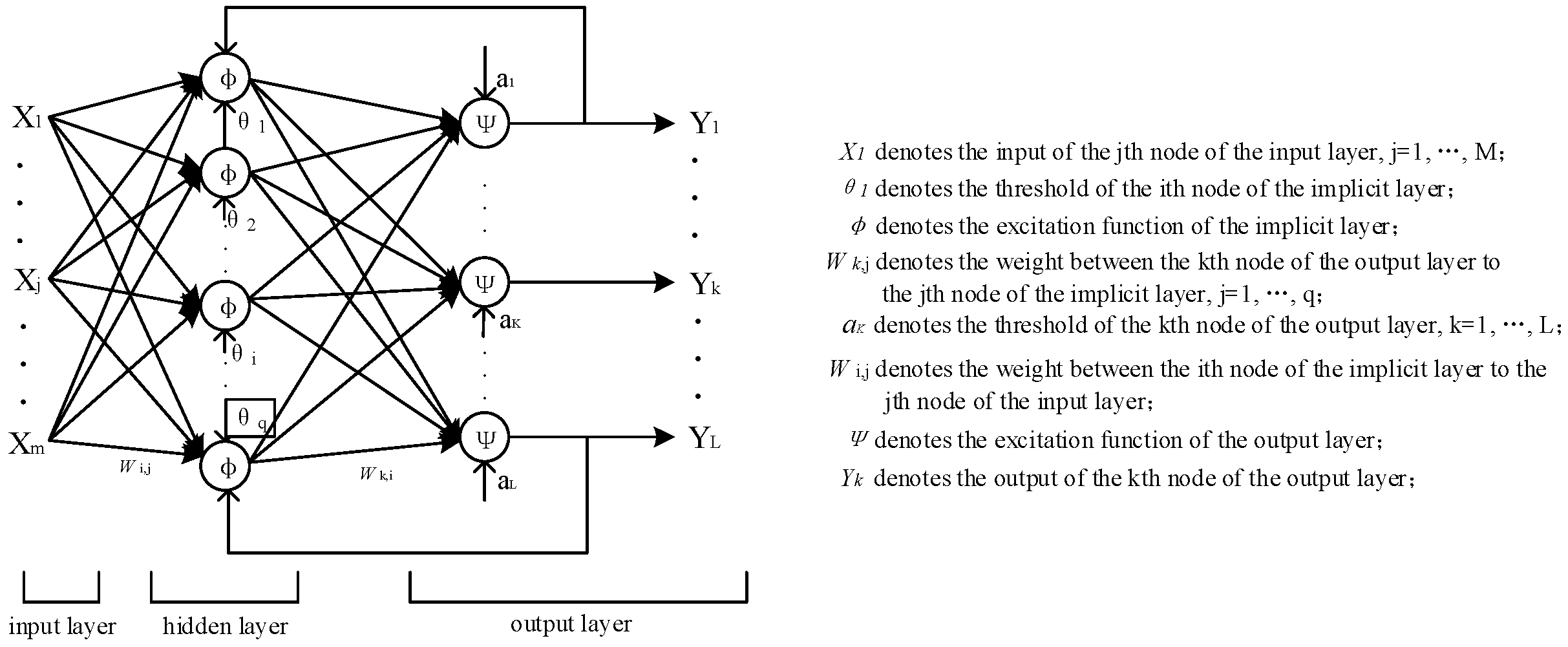
2.1. BP Neural Network Principle

BP neural network is a multi-layer feedforward neural network trained by error backpropagation algorithm, which repeatedly adjusts the weights and thresholds of the network through backpropagation process to minimize the difference between the output value and the true value [17]. The topology structure of the BP neural network model includes an input layer, a hidden layer, and an output layer. The hidden layer can have one or more layers, and the layers are fully interconnected. The basic structure is shown in Figure 1 [18]. In the figure, two types of signals propagate between layers, namely signal forward propagation and error backpropagation, based on the difference between the input and weight functions and the actual output value and expected value of the network. In the forward propagation process, the input vector starts from the hidden layer, is calculated layer by layer through the hidden layer, and then transmitted to the output layer, and the state of each layer of neurons only affects the state of the next layer of neurons. When the output layer cannot obtain the expected value, it will enter the error backpropagation process, and the error signal will return along the original route, gradually adjusting the weights and thresholds of each layer of the network until the input layer and then repeating iterative calculations.

The specific operation steps are as follows.

1. Select training samples and test samples to provide to the network;

2. Positive propagation:

(1) The input net_i of the i-th node in the hidden layer:

$$ne{t}_i={\sum }_{j=1}^M{\omega }_{ij}{x}_j+{\theta }_i.$$

(1)

(2) The output Y_i of the i-th node in the hidden layer:

$$Y_i=\Phi \left(ne{t}_i\right)=\Phi \left({\sum }_{j=1}^M{\omega }_{ij}{x}_j+{\theta }_i\right).$$

(2)

The commonly used activation functions include Sigmoid function and ReLU function.

(3) The input net_k of the kth node in the output layer is

$$ne{t}_k={\sum }_{i=1}^q{\omega }_{ki}{y}_i+a_k={\sum }_{i=1}^q{\omega }_{ki}\Phi \left({\sum }_{j=1}^M{\omega }_{ij}{x}_j+{\theta }_i\right)+a_k.$$

(3)

(4) The output of the kth node in the output layer, Y_k, is

$$Y_k=\psi \left(ne{t}_k\right)=\psi \left({\sum }_{i=1}^q{\omega }_{ki}\Phi \left({\sum }_{j=1}^M{\omega }_{ij}{x}_j+{\theta }_i\right)+a_k\right).$$

(4)

3. Backpropagation:

(1) The error function of the output layer is defined as

$$E={\displaystyle \frac{1}{2}}{\sum }_{k=1}^L{\left(z_k-y_k\right)}^2.$$

(5)

(2) The total error function of the system for the training samples is

$$E={\displaystyle \frac{1}{2}}{\sum }_{p=1}^p{\sum }_{k=1}^L{\left(z_k-y_k\right)}^2.$$

(6)

(3) Correct the ownership values and thresholds obtained from the output layer and hidden layer:

$$\Delta {\omega }_{ki}=-\eta {\displaystyle \frac{\partial E}{\partial {\omega }_{ki}}}=-\eta {\displaystyle \frac{\partial E}{\partial ne{t}_k}}{\displaystyle \frac{\partial ne{t}_k}{\partial w_{ki}}}=-\eta {\displaystyle \frac{\partial E}{\partial y_k}}{\displaystyle \frac{\partial y_k}{\partial ne{t}_k}}{\displaystyle \frac{\partial ne{t}_k}{\partial w_{ki}}}$$

(7)

$$\Delta a_k=-\eta {\displaystyle \frac{\partial E}{\partial a_k}}=-\eta {\displaystyle \frac{\partial E}{\partial ne{t}_k}}{\displaystyle \frac{\partial ne{t}_k}{\partial a_k}}=-\eta {\displaystyle \frac{\partial E}{\partial y_k}}{\displaystyle \frac{\partial y_k}{\partial ne{t}_k}}{\displaystyle \frac{\partial ne{t}_k}{\partial a_k}}$$

(8)

$$\Delta {\omega }_{ij}=-\eta {\displaystyle \frac{\partial E}{\partial {\omega }_{ij}}}=-\eta {\displaystyle \frac{\partial E}{\partial ne{t}_i}}{\displaystyle \frac{\partial ne{t}_i}{\partial {\omega }_{ij}}}=-\eta {\displaystyle \frac{\partial E}{\partial y_i}}{\displaystyle \frac{\partial y_i}{\partial ne{t}_i}}{\displaystyle \frac{\partial ne{t}_i}{\partial {\omega }_{ij}}}$$

(9)

$$\Delta {\theta }_i=-\eta {\displaystyle \frac{\partial E}{\partial {\theta }_i}}=-\eta {\displaystyle \frac{\partial E}{\partial ne{t}_i}}{\displaystyle \frac{\partial ne{t}_i}{\partial {\theta }_i}}=-\eta {\displaystyle \frac{\partial E}{\partial y_i}}{\displaystyle \frac{\partial y_i}{\partial ne{t}_i}}{\displaystyle \frac{\partial ne{t}_i}{\partial {\theta }_i}}.$$

(10)

The organized formula is

$$\Delta {\omega }_{ki}=\eta {\sum }_{p=1}^p{\sum }_{k=1}^L\left(z_k^p-y_k^p\right)\cdot {\psi }^{\prime }\left(ne{t}_k\right)\cdot y_i$$

(11)

$$\Delta a_k=\eta {\sum }_{p=1}^p{\sum }_{k=1}^L\left(z_k^p-y_k^p\right)\cdot {\psi }^{\prime }\left(ne{t}_k\right)$$

(12)

$$\Delta {\omega }_{ij}=\eta {\sum }_{p=1}^p{\sum }_{k=1}^L\left(z_k^p-y_k^p\right)\cdot {\psi }^{\prime }\left(ne{t}_k\right)\cdot {\omega }_{ki}{\Phi }^{\prime }\left(ne{t}_i\right)\cdot x_i$$

(13)

$$\Delta {\theta }_i=\eta {\sum }_{p=1}^p{\sum }_{k=1}^L\left(z_k^p-y_k^p\right)\cdot {\psi }^{\prime }\left(ne{t}_k\right)\cdot {\omega }_{ki}{\Phi }^{\prime }\left(ne{t}_i\right).$$

(14)

The BP neural network algorithm is widely used because of its simple operation and strong parallelism, but because it chooses the fastest descent method in nonlinear programming and modifies the weight according to the negative gradient direction of the error function, it has problems such as slow convergence speed and easy to fall into a local minima state. Therefore, this article uses the GA to optimize its weights and thresholds to solve the above problems and improve the prediction accuracy of the network model.

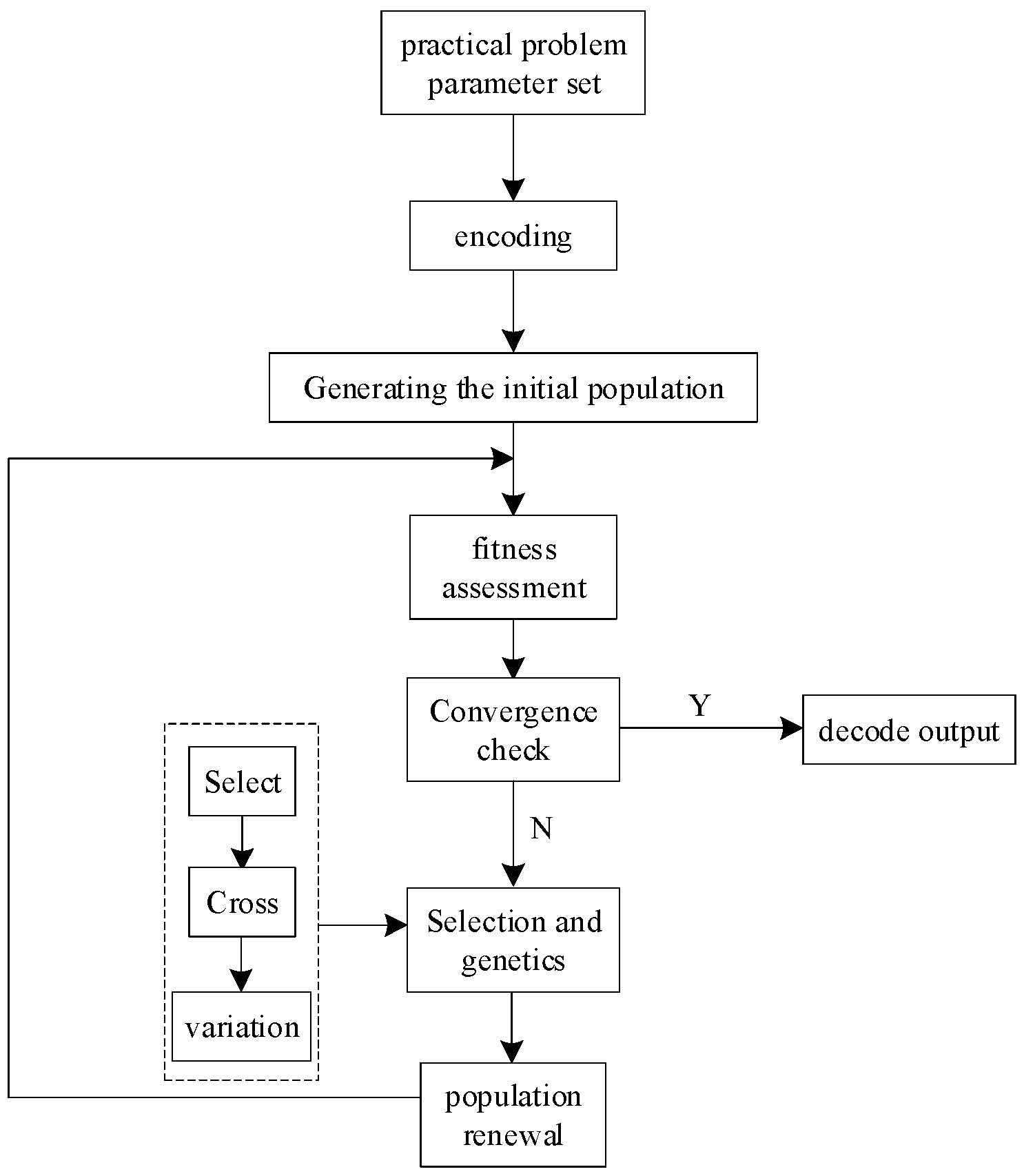
2.2. Principles of Genetic Algorithm

Genetic algorithm imitates the evolutionary mechanisms of biological selection, crossover, and mutation to find the most suitable individuals. It is a random search algorithm that can solve optimization problems for both discrete and continuous functions. In genetic algorithms, the solution to each problem is called a string of chromosomes, typically represented as a bit string, and each chromosome is referred to as an individual. This algorithm adopts a population organization search method, where these populations (chromosome strings) are composed of several individuals, and the individuals are composed of units that control one or more genetic features. The genes for certain features are distributed along the chromosome, and the corresponding strings are called loci. Each genotype represents a potential solution to a problem, which is obtained by mapping chromosome representations to the decision variable space through fitness functions [19]. Algorithms usually preset four operating parameters: population size, evolutionary generation, crossover probability, and mutation probability. When the preset parameter limits are reached, the algorithm will automatically stop. The basic process of classical genetic algorithms is shown in Figure 2.

The specific operation steps are as follows.

(1) Genetic Algorithm Encoding

In genetic algorithm optimization of BP neural network algorithm, each chromosome is decomposed into two parts: connecting genes and parameter genes, and different encoding methods are adopted for these two parts. Encoding is a method of transforming feasible solutions of a problem from its solution space to the search space that the algorithm can handle using genetic algorithms. It is the first problem to be solved when using genetic algorithms. Meanwhile, encoding also affects the operations of selection, crossover, and mutation operators during the operation of genetic algorithms.

(2) Design of fitness function

The fitness function, also known as the evaluation function, in genetic algorithms is the only method to determine the quality of solutions by judging the degree of superiority or inferiority of individuals in the population based on the objective function of the problem being solved. It has a direct impact on the convergence speed of the algorithm and the search for the optimal solution. In the process of searching evolution, genetic algorithms use fitness function values to measure the degree to which each individual in the population can achieve or approach finding the optimal solution in optimization calculations. The fitness function in this article is based on the total error of the neural network and is expressed as follows:

$$f={\displaystyle \frac{1}{\left(1+E\right)}}.$$

(15)

Among them, $E$ is the total error in the network structure, $Z_j^k$ is the ideal output, $Y_j^k$ is the actual output, and K is the number of sample sets.

(3) Genetic operator design

Genetic operations include three basic genetic operators: selection, crossover, and mutation.

(1) The operation of finding excellent individuals from a group and eliminating inferior individuals is called selection. The purpose of selection is to directly pass on optimized individuals or solutions to the next generation or generate new individuals through paired crossover and then pass them on to the next generation. This operation is based on the assessment of individual fitness in the population. The selection operator in this article adopts the most commonly used and simplest roulette wheel selection in genetic algorithms.

The roulette wheel selection first calculates the selection probability of each individual, and the steps are as follows.

① Calculate the sum of fitness values for all individuals in the population:

$$F={\sum }_{K=1}^{M}Eval\left({\nu }_k^{\prime }\right),k=1,2,\dots ,M.$$

(16)

Among them,

F is the sum of the fitness values of all individuals in the group;

M is the number of individuals in the group;

$Eval\left({\nu }_k^{\prime }\right)$ is the fitness value of the kth individual in the population.

② Calculate the selection probability for each chromosome:

$$p_k={\displaystyle \frac{Eval\left(v_k^{\prime }\right)}{F}}.$$

(17)

Among them, p_k is the selection probability of the kth chromosome.

After calculating the selection probability of each chromosome, construct a disk and divide it into N sectors, with the center angle of the Kth sector being 2π$p_k$. Then, imagine a pointer pointing to the junction of the first sector and the Nth sector. Rotate the disk counterclockwise M times, with each rotation. When the disk stops rotating, if the pointer points to the kth sector, select the kth chromosome. When the pointer points to the boundary between the kth sector and the k+1st sector, the kth chromosome is selected. In the algorithm implementation of roulette wheel selection, a random number r from [0, 1] is used to simulate the position pointed by the pointer after the disk stops rotating, and the sector pointed by the pointer is determined by calculating the cumulative probability of each chromosome ${\nu }_k$.

(2) The crossover operator plays a core role in genetic algorithms, which replaces and recombines partial structures of two parent individuals to generate new individuals. Through this operation, the search ability of genetic algorithms can be greatly improved. The commonly used crossover operators include single-point crossover, two-point crossover, multi-point crossover, and uniform crossover. In this article, single-point crossover is used. The so-called single-point crossover refers to randomly selecting a crossover point among individuals and then swapping the substrings of two parents on the right side of the hybridization point to generate two offspring.

In genetic algorithm, single-point crossover first selects several chromosomes from the population generated by roulette wheel selection with a certain probability as the parent, and then generates M random numbers from [0, 1]. If the probability of selecting the parent is greater than or equal to the generated random number, the chromosome corresponding to the random number in the population is selected as the parent. If the selected parents are an odd number, then randomly select another parent from the group, or delete one from the already selected parents. Thus, select an even number of parents and cross them pairwise.

(3) The basic content of mutation operators is to change the gene values on certain loci of individual strings in a population with the aim of introducing chromosome diversity in the population and preventing immature convergence of the algorithm. According to different encoding representations of individuals, it can be divided into real valued variation and binary variation. The operation process of the mutation operator in genetic algorithm is to generate a random number r for each gene locus of each chromosome in the population after hybridization. If $r\le p_m$, the gene locus is mutated, otherwise no mutation is performed.

Before the evolution of genetic algorithms, the solution of the solution space was represented as genotype string structure data of genetic algorithms, and different combinations of these string structure data constituted different loci. After setting the 4 operating parameters, the algorithm will randomly generate N individuals as the initialized population, reflect the advantages and disadvantages of the individual or solution through the appropriate fitness function, and then use three genetic operators, namely selection, crossover and mutation to form a new population with excellent individuals, and then return to the fitness assessment step. When the convergence criterion is reached, the algorithm automatically stops iteration and terminates the operation.

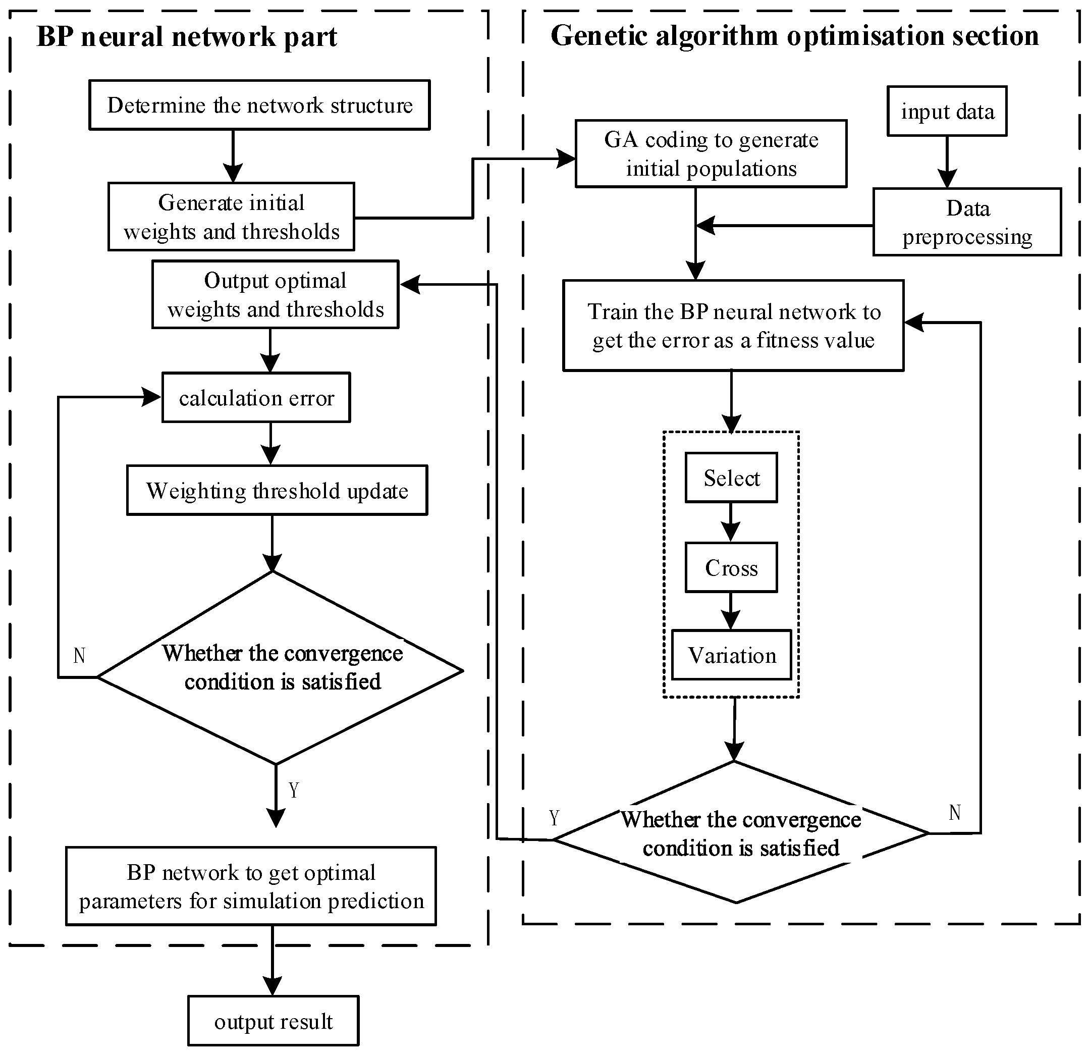
2.3. Construction of the GA–BP Neural Network Model

As a random search algorithm, the genetic algorithm has a strong global merit ability and robustness, which can optimize the weights and thresholds of BP neural networks, which are mainly divided into three parts: the determination of the structure of the BP neural network, the optimization of weights and thresholds of genetic Algorithms, and the training and prediction of BP neural networks. In this paper, the genetic algorithm is used to optimize the initial weights and thresholds of the BP neural network. The optimal weights and thresholds are obtained, and the optimal weights and thresholds are then applied to the BP neural network for training, which can prevent the network from falling into local optimization and improve the training performance. For most problems, the BP neural network with a three-layer structure is sufficient, so a three-layer neural network is selected in this paper, including the input layer, the hidden layer, and the output layer. In the following example, the number of engineering characteristic factors of property reduction in the vector of the rough set is the input layer, per square meter cost of the project is the output layer node, and the hidden layer node N is determined according to the empirical formula, where N is the number of hidden layer nodes, m is the number of neuron nodes of the input layer, and n is the number of output layer neuron nodes, which is $N=\sqrt{m+n}+\alpha$, $\alpha$, a constant between them [1, 10]. Based on the above theory, the steps of genetic algorithm to optimize BP neural network are as follows.

(1) After determining the topology of the neural network, initial weights and thresholds are generated. They are expressed in the BP neural network in the form of vectors, including the vectors composed of the connection weights W_1j,…, W_ij between the input layer and the hidden layer, the vectors composed of hidden layer threshold θ₁, …, θ_i, the vectors composed of the connection weights W_2j, …, W_kj between the hidden layer and the output layer, and the vectors composed of the threshold of the output layer a1, …, ak.

(2) Determine the fitness function. The selection of the fitness function is determined by the minimum mean square error between the obtained test set and the training set by the BP neural network on the data, and the smaller the error, the higher the accuracy.

(3) Determine the global search operator of the algorithm. The roulette method is used to select individuals with good fitness from the population. Two chromosomes are randomly selected from the population, a cross point is randomly generated at the same time, the other half of the two chromosomes is exchanged to obtain the two newly generated individuals, and their feasibility is tested. For the mutation operation, one individual is randomly selected and a mutation point is randomly selected, and the mutation is carried out according to a certain probability, so as to produce a new individual [20].

(4) If the obtained neural network weights and thresholds do not meet the convergence conditions, return to step (1) and iterate again.

(5) After obtaining the optimal weights and thresholds of the BP neural network, they are assigned to the BP neural network for optimized training and prediction to obtain the final results.

Figure 3 shows the process.

3. Determination of Engineering Eigenvectors

It can be seen from the “Investment Estimation Index of Prefabricated Construction Engineering” that the index base price of investment estimation of prefabricated concrete structure engineering is composed of construction engineering cost, installation engineering cost, equipment purchase cost, other engineering construction costs, and basic preparation costs. Also, the proportion of construction and installation engineering cost to the index base price is over 80%. The selection of engineering features directly affects the prediction accuracy of the model, which should reflect not only the basic characteristics of the project, but also the core parameters that affect the cost of the project. According to the research of Hu Guoqing et al. [21], it shows that the cost-significant items (CSIs) of prefabricated buildings are reflected primarily in four projects: cast-in-place reinforced concrete engineering, PC component and installation, decoration engineering, and water supply and drainage engineering., The cost of these four CSIs represents more than 85% of the total cost. Therefore, based on analyzing the cost composition of traditional buildings and prefabricated building projects, this article preliminarily screens out 11 characteristic parameters that affect the estimation of investment estimation of prefabricated buildings by reviewing the literature [16,22,23]: foundation type, structure type, construction area, number of building floors, prefabricated component type, prefabricated component connection method, roofing and waterproofing, decoration engineering, installation, electrical and water supply and drainage engineering, assembly rate, and project cost index.

Rough set theory is the work of the Polish scholar Z. Pawlak, proposed in 1982. It can deal with the problems of data simplification and inconsistent information analysis on the premise of retaining information. It has been widely used in machine learning, knowledge acquisition, decision analysis, and other fields [22]. To avoid the problem of data redundancy caused by too many factors of engineering features, this paper adopts rough set theory to reduce the dimension of engineering feature indicators and improve the speed of the neural network. Since the attribute values in the decision table of rough set theory need to be discretized, the above qualitative features are quantified in this paper, and the quantitative results are shown in

Table 1. Quantification of characteristics of prefabricated building projects.

Engineering Features	Quantify the Value
	1	2	3	4	5
Foundation type	Independent foundation	Raft foundation	Strip foundations	Pile foundations
Structure type	Shear wall structure	Frame structure	Frame shear wall structure	Tube structure	Prefabricated containerized structure
Area	Enter based on actual data, unit: m2
Number of floors of the building	Enter based on actual data
The Type of prefabricated component	Prefabricated laminated floor slabs	Prefabricated sandwich insulated exterior wall panels	Prefabricated interior wall panels	Prefabricated stairs	Prefabricated air conditioning panels
Prefabricated component connections	Grouting rebar sleeve connection	Reinforcement slurry anchor lap connection
Roofing and waterproofing	Flat roof Class 1 waterproof	Flat roof Class 2 waterproof	Flat roof Class 3 waterproof	Pitched roof Class 1 waterproof	Curved roofs Class 1 waterproof
Decoration works	Simple decoration	Standard finish	Mid-range finish	High-end decoration
Installation, Electrical and Water Supply and Drainage Engineering/(Yuan·m−2).	Enter based on actual data
Assembly rate/%.	Enter based on actual data
Project cost index	Enter based on actual data

.

The decision table is an important knowledge expression system in rough set theory. The basic structure of the decision table in this paper is based on engineering characteristic factors as conditional attributes, and the unilateral cost of prefabricated engineering as the decision attribute. By referring to prefabricated construction engineering case studies [24,25] and collecting information on some newly built prefabricated construction projects, 16 sets of prefabricated construction project data from central and southern China were finally compiled for network training, including 15 sets as training samples and 1 set as a testing sample. Due to the confidentiality of some information in the construction project, it is required not to disclose the company and project to which it belongs. Therefore, this article combines the complete actual engineering case information collected offline with the data cited in the literature. At the same time, the Boolean reasoning algorithm in the Rosetta rough set software, adapted to Windows 2000/XP version, is used to discretize the six continuous variables of building area, building floors, installation, electrical and plumbing engineering, assembly rate, engineering cost index, and decision attribute engineering unit cost in the conditional attributes, and it establishes an initial decision table, as shown in

Table 2. Initial decision table.

Sample No.	Conditional Attributes											Decision Attributes
	Foun-dation Type	Struc-ture Type	Area	Number of Floors of the Building	The Type of Prefabric-ated Component	Prefabricated Component Connections	Roofing and Waterproofing	Decoration Works	Installation, Electrical and Water Supply and Drainage Works (RMB/m2).	Asse-mbly rate (%)	Project Cost Index	Cost per Square Meter (RMB/m2)
1	4	1	1	2	1 + 4 + 5	1	1	1	3	1	2	3
2	1	1	3	4	1 + 3	1	1	2	1	4	3	1
3	2	1	3	1	1 + 2 + 3 + 4	1	1	2	3	2	3	5
4	2	1	1	2	1 + 2 + 3 + 4	2	1	2	1	1	2	4
5	2	4	3	1	1 + 2 + 3	1	1	1	3	1	3	2
6	1	1	3	4	1 + 3	2	1	2	1	4	2	1
7	2	1	1	2	1 + 2 + 3	1	1	2	1	1	2	3
8	2	3	5	3	1 + 4	1	2	1	5	1	2	3
9	2	3	3	2	1 + 4	1	2	1	5	4	2	5
10	4	1	2	1	1 + 4 + 5	1	1	1	1	1	2	2
11	2	4	4	2	1 + 2 + 3	1	1	2	1	1	3	1
12	2	1	1	1	1 + 2 + 3	1	4	2	1	1	3	2
13	1	1	5	4	1 + 2 + 3	2	4	2	1	1	3	2
14	2	1	2	1	1 + 2 + 3	1	1	2	1	1	3	1
15	2	1	4	2	1 + 3	1	1	2	3	4	3	2
16	2	1	3	2	1 + 3	1	1	1	1	2	3	2

.

Once the initial decision table is established, genetic algorithm reduces its properties, and the results are shown in

Table 3. Brief table of initial engineering characteristics.

Initial Features	Frequency	Initial Features	Frequency
Base type	8	Structure type	9
Area	21	Number of floors of the building	16
The Type of prefabricated component	16	Prefabricated component connections	21
Roofing and waterproofing	17	Decoration works	14
Installation, electrical and plumbing works	12	Assembly rate	14
Project cost index	17

[26]. Then, select the frequency of ≥14 in the table as the main engineering feature index and use it as the input vector of the neural network.

4. Case Studies

4.1. Neural Network Data Preprocessing

Due to the significant differences and inconsistent units in the data of the main engineering feature indicators, the learning speed and prediction accuracy of the neural network are greatly limited. Therefore, the normalization formula is used to preprocess the data in

Table 4. Data table of sample indicators of main engineering characteristics.

Sample Number	Area	Number of Floors of the Building	The Type of Prefabricated Component	Prefabricated Component Connections	Roofing and Waterproofing	Decoration Works	Assembly Rate (%)	Project Cost Index	Cost per Square Meter (RMB/m2)
1	21,749	25	1 + 4 + 5	1	1	1	51	100	2033.03
2	13,841	18	1 + 3	1	1	2	50	105	2079.71
3	22,164	33	1 + 2 + 3 + 4	1	1	2	65	109	2286.57
4	20,020	30	1 + 2 + 3 + 4	2	1	2	68	113	2265.35
5	23,860	33	1 + 2 + 3	1	1	1	63	105	2104.47
6	14,638	18	1 + 3	2	1	2	50	113	1997.14
7	19,908	30	1 + 2 + 3	1	1	2	62	113	2195.35
8	3167	6	1 + 4	1	2	1	30	100	2805
9	15,733	27	1 + 4	1	2	1	32	100	2743
10	20,453	34	1 + 4 + 5	1	1	1	51	100	2192.68
11	16,451	27	1 + 2 + 3	1	1	2	60	105	2094.53
12	20,246	33	1 + 2 + 3	1	4	2	60	109	2153.62
13	12,881	18	1 + 2 + 3	2	4	2	60	105	2135.28
14	21,468	33	1 + 2 + 3	1	1	2	58	109	2076.81
15	18,200	27	1 + 3	1	1	2	50	105	2006.45
16	19,309	30	1 + 3	1	1	1	55	109	2073.73

, mapping the row minimum and maximum values to [−1, 1] to process the input engineering feature vectors. The processing results are shown in

Table 5. Normalization table of sample data of main engineering characteristic indicators.

Sample Number	Area	Number of Floors of the Building	The Type of Prefabricated Component	Prefabricated Component Connections	Roofing and Waterproofing	Decoration Works	Assembly Rate (%)	Project Cost Index	Cost per Square Meter (RMB/m2)
1	0.796	0.357	1.000	−1.000	−1.000	−1.000	0.105	−1.000	−0.911
2	0.032	−0.143	−1.000	−1.000	−1.000	1.000	0.053	−0.231	−0.796
3	0.836	0.929	1.000	−1.000	−1.000	1.000	0.842	0.385	−0.283
4	0.629	0.714	1.000	1.000	−1.000	1.000	1.000	1.000	−0.336
5	1.000	0.929	−0.333	−1.000	−1.000	−1.000	0.737	−0.231	−0.734
6	0.109	−0.143	−1.000	1.000	−1.000	1.000	0.053	1.000	−1.000
7	0.618	0.714	−0.333	−1.000	−1.000	1.000	0.684	1.000	−0.509
8	−1.000	−1.000	−0.667	−1.000	−0.333	−1.000	−1.000	−1.000	1.000
9	0.215	0.500	−0.667	−1.000	−0.333	−1.000	−0.895	−1.000	0.847
10	0.560	0.714	−1.000	−1.000	−1.000	−1.000	0.316	0.385	−0.810
11	0.284	0.500	−0.333	−1.000	−1.000	1.000	0.579	−0.231	−0.759
12	0.651	0.929	−0.333	−1.000	1.000	1.000	0.579	0.385	−0.613
13	−0.061	−0.143	−0.333	1.000	1.000	1.000	0.579	−0.231	−0.658
14	0.769	0.929	−0.333	−1.000	−1.000	1.000	0.474	0.385	−0.803
15	0.453	0.500	−1.000	−1.000	−1.000	1.000	0.053	−0.231	−0.977
16	0.671	1.000	1.000	−1.000	−1.000	−1.000	0.105	−1.000	−0.516

:

$$X^{\prime }={\displaystyle \frac{x_{min}}{x_{max}-x_{min}}}$$

(18)

4.2. Model Simulation and Comparative Analysis

Using MATLAB R2019a software, 15 sets of sample data were used to optimize the weights and thresholds of the BP neural network through GA genetic algorithm for simulation training, and one set of data was left for prediction verification. The predicted values after fixing the random seeds are shown in

Table 6. GA optimized BP neural network prediction results.

Number	Real Value	Predicted Value	Number	Real Value	Predicted Value
1	2033.03	2092.03	9	2743	2624.79
2	2079.71	2052.06	10	2192.68	2137.67
3	2286.57	2280.84	11	2094.53	2031.71
4	2265.35	2212.65	12	2153.62	2130.39
5	2104.47	1997.63	13	2135.28	2138.09
6	1997.14	2196.37	14	2076.81	2149.30
7	2195.35	2162.74	15	2006.45	2034.42
8	2805	2637.37	Test set	2073.73	2053.40

, and the errors between the training set and the test set are shown in

Table 7. GA optimized BP neural network simulation error table.

Name	MSE	MAE	MAPE (%)
Training set	7657.27	67.60	3.02
Test set	413.49	20.33	0.98

. (Among them, based on empirical formulas, the network prediction model is determined to have 10 hidden layer nodes, and the parameters of GA genetic algorithm are as follows. Population size: 50; maximum iteration number: 30; intersection probability: 0.8; mutation probability: 0.2).

On the basis of optimizing the BP neural network with genetic algorithm, the PSO optimization algorithm was used to predict and analyze the model. The results are shown in

Table 8. PSO optimized BP neural network prediction results.

Number	Real Value	Predicted Value	Number	Real Value	Predicted Value
1	2033.03	2453.59	9	2743	1947.21
2	2079.71	3923.95	10	2192.68	1092.39
3	2286.57	3552.40	11	2094.53	3542.95
4	2265.35	8047.56	12	2153.62	6431.30
5	2104.47	3538.07	13	2135.28	3401.63
6	1997.14	1471.92	14	2076.81	3542.92
7	2195.35	3269.72	15	2006.45	3544.70
8	2805	770.62	Test set	2073.73	2010.36

, and the errors between the training set and the test set are shown in

Table 9. PSO optimized BP neural network simulation error table.

Name	MSE	MAE	MAPE (%)
Training set	4,973,203.32	1751.55	79.29
Test set	4015.43	63.37	3.06

:

Based on the small sample size of this study, stratified k (k = 5) fold cross validation was used, and the optimization results of the two optimization algorithms are shown in

Table 10. Cross-validation results.

Optimization Algorithm	MSE	MAE	MAPE
genetic algorithm	9528.55 ± 8926.31	73.35 ± 44.56	3.3 ± 2.0%
PSO algorithm	1,406,319.31 ± 626,556.23	1123.71 ± 245.06	51.1 ± 9.6%

.

According to Table 10, in the case of a small sample size in this study, the absolute value of the MSE of the genetic algorithm is relatively high, with large fluctuations between different folds. A high MSE standard deviation indicates that the model is sensitive to data partitioning, but the MAPE of the model shows good relative error control. On the other hand, the results of PSO are very poor, and the model can hardly make accurate predictions. Based on this, it can be inferred that genetic algorithms can better adapt to small sample problems by searching the solution space through selection, crossover, and mutation. PSO relies on particle swarm intelligence, which may be difficult to converge in large parameter spaces, especially when there are many local optima in high-dimensional spaces.

The above results are all the results of running the model multiple times. During the simulation process, although the relevant parameters of the model were modified multiple times, the cross-validation results were always unsatisfactory. Therefore, it can be concluded that the optimization performance of genetic algorithm is superior to PSO algorithm in this problem.

5. Conclusions

This article combines prefabricated building investment estimation, rough set theory, and the GA–BP network prediction model. Firstly, based on the collection of factors affecting the characteristics of prefabricated construction engineering, this article uses rough set theory to perform attribute reduction, which improves the prediction accuracy of the GA–BP model while eliminating redundant attributes. Secondly, by normalizing the initial sample data through function operations, the GA–BP neural network model is applied to predict the investment estimation of prefabricated buildings, and the results are compared with the PSO-optimized BP neural network model. The results indicate that the overall prediction accuracy of the GA–BP neural network model in this study is better than that of the PSO-optimized BP neural network, and its prediction results are more stable. It is scientifically effective for estimating and predicting prefabricated buildings in the investment decision-making stage.

The complete investment estimation indicators for prefabricated buildings include equipment purchase costs and other construction costs, among others. As the construction and installation costs of prefabricated buildings account for 80% or more of the base price of the investment estimation prediction indicators for prefabricated buildings, this article only predicts the construction and installation costs of prefabricated buildings. On the other hand, the prediction model of neural networks is built on the basis of obtaining complete information from completed prefabricated construction projects. When collecting relevant data on prefabricated construction projects, this article found that the engineering data information provided by relevant construction units was incomplete, and the information on prefabricated construction projects on relevant construction websites and government regulatory platforms was also incomplete. Therefore, this article suggests that, in actual engineering construction, all participating units should timely exchange engineering information, achieve transparency of engineering information in accordance with principles, and upload it to government regulatory platforms in a timely manner. At the same time, the government should strengthen the supervision of prefabricated construction projects, ensure the timeliness and effectiveness of information uploaded by relevant units participating in prefabricated construction, and improve the database of prefabricated construction. In addition, a BIM-based data platform for the entire lifecycle of prefabricated buildings can be established, integrating data flows from design, production, logistics, and assembly to achieve dynamic mapping of identification codes and cost information.

However, this article still has certain limitations. Firstly, there is the issue of sample size, as a small number of samples may lack certain persuasiveness. Secondly, there is the research methodology. This article uses the genetic optimization algorithm. In future research, if there are sufficient data, deep-learning methods can be introduced for prediction.

References

1. Zhang, M.; Liang, J. Investment Estimation Method of Construction Project in Decision Stage. Pet. Plan. Eng. 2005, 53–55. [Google Scholar]
2. Yan, H.; He, Z.; Gao, C.; Xie, M.; Sheng, H.; Chen, H. Investment estimation of prefabricated concrete buildings based on XGBoost machine learning algorithm. Adv. Eng. Inform. 2022, 54, 101789. [Google Scholar]
3. Liu, M.; Luo, M. Cost estimation model of prefabricated construction for general contractors based on system dynamics. Eng. Constr. Archit. Manag. 2025, 32, 621–638. [Google Scholar]
4. Choi, Y.; Park, C.Y.; Lee, C.; Yun, S.; Han, S.H. Conceptual cost estimation framework for modular projects: A case study on petrochemical plant construction. J. Civ. Eng. Manag. 2022, 28, 150–165. [Google Scholar]
5. Sievers, S.; Seifert, T.; Franzen, M.; Schembecker, G.; Bramsiepe, C. Fixed capital investment estimation for modular production plants. Chem. Eng. Sci. 2017, 158, 395–410. [Google Scholar]
6. Zhang, P.; Dong, Y. Strategy transformation of big data green supply chain by using improved genetic optimization algorithm. Soft Comput. 2023, 1–10. [Google Scholar] [CrossRef]
7. Yunlong, W.; Hao, W.; Guan, G.; Li, K.; Lin, Y.; Chai, S. Intelligent Layout Design of Ship Pipeline Using a Particle Swarm Optimisation Integrated Genetic Algorithm. Int. J. Marit. Eng. 2021, 163. [Google Scholar] [CrossRef]
8. Wang, B.; Yang, C.; Ding, Y. Non-Dominated Sorted Genetic Algorithm-II Algorithm-based Multi-Objective Layout Optimization of Solid Wood Panels. BioResources 2022, 17, 94–108. [Google Scholar]
9. Duan, B.; Guo, C.; Liu, H. A hybrid genetic-particle swarm optimization algorithm for multi-constraint optimization problems. Soft Comput. 2022, 26, 11695–11711. [Google Scholar]
10. Langazane, S.N.; Saha, A.K. Effects of Particle Swarm Optimization and Genetic Algorithm Control Parameters on Overcurrent Relay Selectivity and Speed. IEEE Access 2022, 10, 4550–4567. [Google Scholar]
11. Deep, K.; Thakur, M. Development of a Mutation Operator in a Real- Coded Genetic Algorithm for Bridge Model Optimization. Appl. Math. Comput. 2007, 193, 211–230. [Google Scholar]
12. Kim, G.H.; Yoon, J.E.; An, S.H.; Cho, H.H.; Kang, K.I. Neural network model incorporating a Genetic Algorithm in estimating construction costs. Build. Environ. 2004, 39, 1333–1340. [Google Scholar]
13. Zhou, C. Discussion of Project Investment Estimation Method based on BP Neural Network. Railw. Eng. Cost Manag. 2015, 30, 6–9+13. [Google Scholar]
14. Pan, Y.H.; Zhang, Y.L.; Cai, Y.J.; Wu, H.H.; Sui, H.Y. Research on Highway Engineering Cost Estimation Based on the GA-BP Algorithm. J. Chongqing Jiaotong Univ. (Nat. Sci.) 2016, 35, 141–145. [Google Scholar]
15. Zhang, F.; Liang, X. Research on investment estimation method of urban rail transit project based on GA-ELM. J. Railw. Sci. Eng. 2019, 16, 1842–1848. [Google Scholar]
16. Wang, F.; Zhang, S.; Li, Y. Application of Neural Network Model of BAS-BP in Investment Estimation of Prefabricated Building. J. Anhui Univ. Technol. (Nat. Sci.) 2019, 36, 382–387. [Google Scholar]
17. Rumelhart, D.; Hinton, G.; Williams, R. Learning representations by back-propagating errors. Nature 1986, 323, 533–536. [Google Scholar]
18. MATLAB Technology Alliance; Liu, B.; Guo, H. MATLAB Neural Network Super Learning Manual; Posts & Telecom Press: Beijing, China, 2014; pp. 159–161. [Google Scholar]
19. Scrucca, L. GA: A package for Genetic Algorithms in R. J. Stat. Softw. 2013, 53, 1–37. [Google Scholar]
20. Xiao, Y.; Yang, J.; Zhou, S. Engineering Optimization—Theory, Model and Algorithm; Beihang University Press: Beijing, China, 2021; Volume 1, p. 317. [Google Scholar]
21. Hu, Q.; Cai, B.; He, Z.; Dai, Z. Investment estimation of prefabricated building based on BP neural network. J. Chang. Univ. Sci. Technol. (Nat. Sci.) 2018, 15, 66–72+86. [Google Scholar]
22. Han, Z.; Zhang, Q.; Wen, F. Rough sets: Theory and application. Inf. Control 1998, 38–46. [Google Scholar]
23. Hu, Q.; Tian, X.; He, Z. Green building investment estimation method based on genetic algorithm optimized extreme learning machine. Build. Econ. 2020, 41, 125–130. [Google Scholar]
24. Xia, F.; Fang, S.; Chen, P. Typical Project Case About Prefabricated Building. Hous. Sci. 2015, 35, 18–23. [Google Scholar]
25. Zhao, W.; Wang, S. Research on the Investment Estimation of Prefabricated Building Based on BASBP Model. J. Anhui Univ. Sci. Technol. (Nat. Sci.) 2020, 40, 73–79. [Google Scholar]
26. Xu, W.; Shen, J.; Chen, X.; Wan, S. Construction cost prediction model based on RS-RBFNN. J. Qingdao Univ. Technol. 2021, 42, 96–102. [Google Scholar]
Figure 1. Structure diagram of a typical three-layer BP neural network.
Applsci 15 03474 g001
Figure 2. Genetic Algorithm flow chart.
Applsci 15 03474 g002
Figure 3. Flow diagram of the GA–BP neural network.
Applsci 15 03474 g003