Article

Application of 4PCS and KD-ICP Alignment Methods Based on ISS Feature Points for Rail Wear Detection

School of Mechanical Engineering, Hebei University of Science and Technology, Shijiazhuang 050018, China
*
Author to whom correspondence should be addressed.
Appl. Sci. 2025, 15(7), 3455; https://doi.org/10.3390/app15073455
Submission received: 15 February 2025 / Revised: 18 March 2025 / Accepted: 20 March 2025 / Published: 21 March 2025

Abstract

:
In order to detect the abrasion of rails, a new point cloud alignment method combining 4-points congruent sets (4PCS) coarse alignment based on internal shape signature (ISS) and K-dimensional iterative closest points (KD-ICP) fine alignment is proposed, and for the first time, the combined algorithm is applied to the detection of rail wear. Due to the large amount of 3D rail point cloud data collected by the 3D line laser sensor, the original data are first downsampled by voxel filtering. Then, ISS feature points are extracted from the processed point cloud data for 4PCS coarse alignment, and the feature points are quantitatively analyzed, which in turn provides good alignment conditions for fine alignment. Then, the K-dimensional tree structure is used for the near-neighbor search to improve the alignment efficiency of the ICP algorithm. Finally, the total rail wear is calculated by combining the fine alignment results with the wear calculation formula. The experimental results show that when the number of ISS feature points extracted is 4496, the 4PCS coarse alignment algorithm based on ISS feature points is higher than the original 4PCS algorithm as well as the other algorithms in terms of alignment accuracy; the ICP fine alignment algorithm based on the kd-tree is less than the original ICP algorithm as well as the other algorithms in terms of the time consumed. Further, the proposed new ISS-4PCS + KD-ICP two-stage point cloud alignment method is superior to the original 4PCS + ICP algorithm both in terms of alignment accuracy and runtime. The combined algorithm is applied to the detection of rail wear for the first time, which provides a reference for the non-contact rail wear detection method. The high accuracy and low time consumption of the proposed algorithm lays a good foundation for the calculation of rail wear in the next step.

1. Introduction

Railroads, as an important national transportation infrastructure, play an irreplaceable role both in the travel of the population and in the transportation of goods. With the increase in the speed of high-speed railcars and the frequent operation of trains, the detection of rail abrasion has been increasingly emphasized. Rail abrasion, as a key track geometric parameter, plays a vital role in later line maintenance and overhaul formulation [1]. Wear and tear of rails can lead to changes in the contact relationship between wheels and rails, reducing the service life of rails as well as vehicles, increasing operating costs, and leading to crises in life safety [2]. In order to ensure the safety and reliability of railroads, the accurate detection of rail wear is particularly important.
At present, rail wear detection is mainly divided into two kinds, namely contact and non-contact. Contact detection requires railroad staff to use detection tools to manually measure the rail head data, such as the common Mini Prof rail wear detector [3]. But issues in the use of this method include the low efficiency of detection, low reliability, and the fact that it has not been adapted to the current requirements for rail wear detection [4]. Non-contact detection is divided into passive detection and active detection according to the different imaging methods. In this case, passive detection is the establishment of a binocular vision system to make measurements, and active detection is the use of structured light to make measurements [5]. Both have the advantage of fast measurement speed and high measurement accuracy [6]. In particular, 3D line structured light has been widely used in object detection due to its large measurement range, large amount of collected data, and ability to comprehensively obtain the 3D point cloud data of the object under test [7].
The 3D point cloud of the rail obtained by 3D line structured light needs to be aligned with the complete 3D point cloud of the rail before calculating the wear of the rail. Point cloud alignment is the data processing process of adjusting two pieces of point clouds at different positions in the same space to the same position through coordinate transformation. Since the alignment effect cannot be optimized at one time, it is usually divided into two stages: coarse alignment and fine alignment [8]. Coarse alignment allows the two pieces of point clouds at the initial spatial position to be roughly aligned by coordinate transformation, while fine alignment aims to achieve further alignment on the basis of the coarse alignment [9] in order to achieve minimization of the alignment error.
Coarse alignment is divided into two methods, one based on feature points and the other based on global search [10]. The coarse alignment based on feature points is mainly carried out by extracting the corresponding feature information in the two point clouds, of which the most common ones are the Scale-Invariant Feature Transform (SIFT) algorithm [11], the Harris3D feature point algorithm [12], and the internal shape signature (ISS) algorithm [13]. As for the alignment algorithm based on global search, Chen Yi et al. [14] proposed a Principal Component Analysis (PCA) algorithm based on contour distance improvement to realize efficient point cloud auto alignment. Zhang Han et al. [15] proposed an improved Sample Consistent Initial Alignment (SAC-IA) algorithm using geometric constraints via the scan angle limiting method. Aiger et al. [16] proposed a 4-points congruent sets (4PCS) algorithm using 4-points sets corresponding to point congruence properties, which reduces the time complexity of the algorithm. Mellado et al. [17] improved the 4PCS by proposing the Super-4PCS algorithm, which further reduced the time complexity of the 4PCS algorithm, and Pascal et al. [18] proposed the K-4PCS algorithm in order to better adapt to the characteristics of laser scanning. In the fine alignment stage, the most widely used are those based on the Normal Distribution Transformation (NDT) [19] algorithm and those based on the Iterative Closest Point (ICP) [20] algorithm. The ICP algorithm needs to be iterated, and when the quantity of point cloud data is large enough, the algorithm will take longer. In order to solve this time-consuming problem, researchers have conducted a significant amount of research. Chen J et al. [21] proposed the HT-ICP algorithm, which reduces the computation time by eliminating the incorrectly corresponding point pairs. Segal et al. [22] proposed the GICP algorithm, which improves the accuracy of the algorithm through the introduction of oriented quantities and curvature geometric features. Shen Chen et al. [23] used the kd-tree accelerated ICP algorithm on robot disassembly targets to realize point cloud fine alignment.
Due to the large amount of data obtained from rail collection, the time complexity of point cloud alignment tends to be high, which makes the algorithm suffer in terms of both operation efficiency and alignment accuracy [
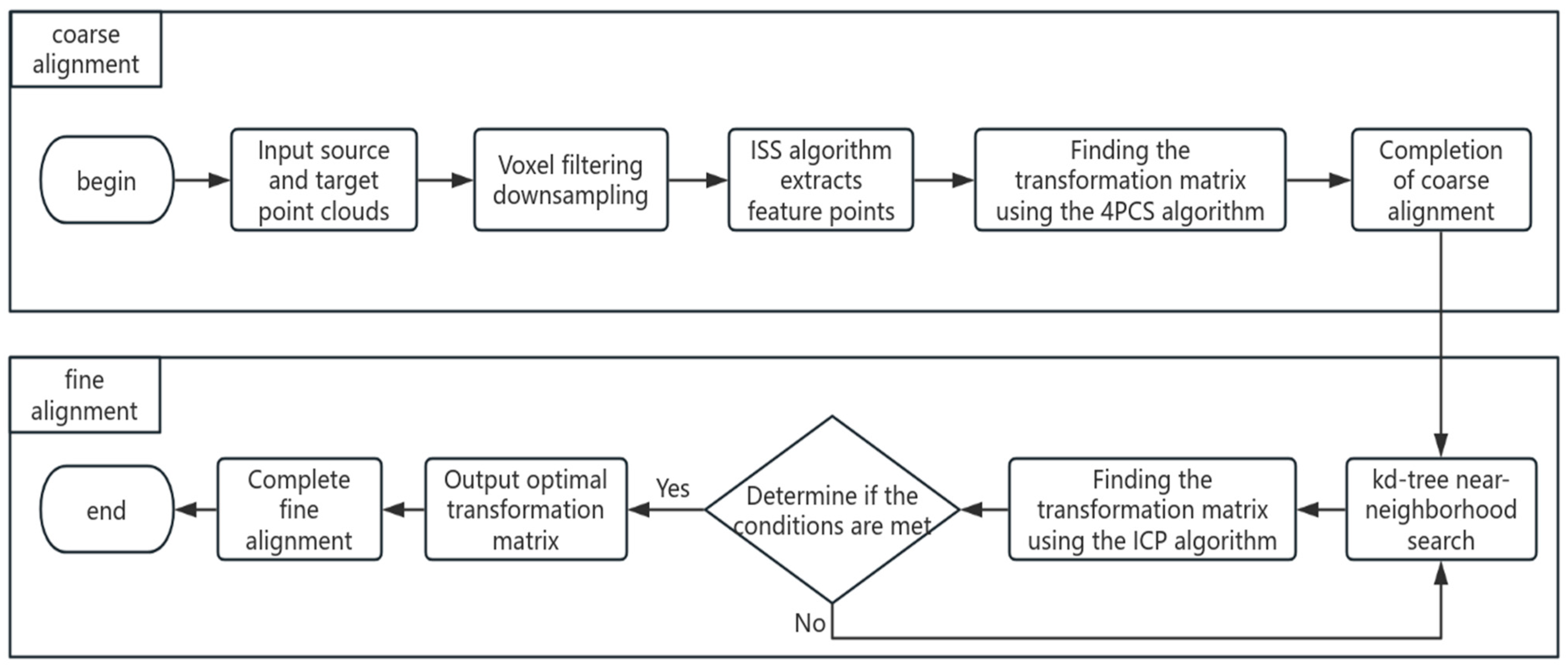
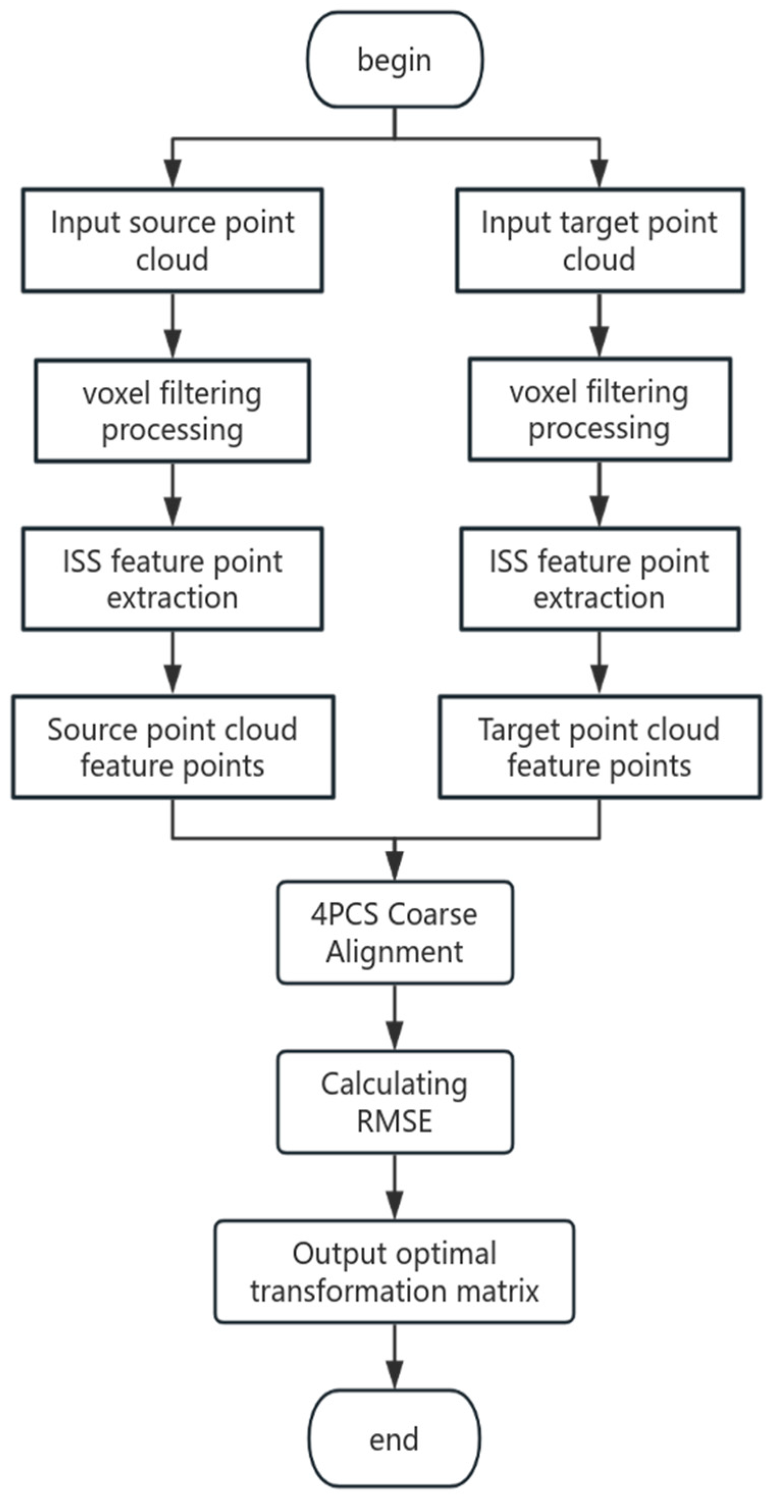
24]. To address the above problems, a point cloud alignment method combining ISS-4PCS and KD-ICP is proposed in this work. That is, ISS feature points are integrated on the basis of the 4PCS algorithm, a 4PCS coarse alignment algorithm based on ISS feature points is proposed, and the KD-ICP algorithm proposed by Shen Chen et al. is applied to rail abrasion detection for fine alignment. The method consists of two stages: ISS-4PCS coarse alignment and KD-ICP fine alignment; the specific realization steps are as follows. In the coarse alignment stage, the voxel filtering is used to downsample the source and target point clouds to be aligned, then the ISS feature point extraction algorithm is used to extract the source and target point cloud feature point sets, and finally the 4PCS algorithm is used to complete the coarse alignment. In the fine alignment stage, the kd-tree near-neighborhood search is used to accelerate the ICP algorithm to complete the fine alignment. This method uses the ISS algorithm to extract the feature points to replace the original data points, which can improve the alignment accuracy of 4PCS algorithm; the use of kd-tree to accelerate the ICP algorithm can improve the alignment efficiency of the ICP algorithm, and the flow of the method used is shown in Figure 1. Experiments show that the combined algorithm proposed in this paper has better robustness in rail point cloud alignment.

2. Point Cloud Data Acquisition and Its Pre-Processing

2.1. Point Cloud Data Acquisition

The data acquisition device used in this paper is the ECCO 75 series 3D line laser sensor of Germany SmartRay Company (Wolfratshausen, Germany), and its related parameters are shown in Table 1. The sensor uses laser triangulation: the laser line is first struck onto the object to be measured, which then reflects the beam back to the image sensor. The 3D sensor receives the offset of the reflected beam from the image sensor and, according to the constant change in the height of the object to be measured, determines the different positions of the reflected beam presented in the image, thus achieving the measurement of the object’s contour.
Using the 3D line laser sensor and its adapted SR_Starterkit 5.5.0.91 software, the data acquisition was carried out on the 60 model rail, setting the laser brightness at 75%, exposure time at 100 μs, the number of image acquisition lines at 100, and the region of interest (ROI) at 1920 × 1200 mm2. The rail profile point cloud data acquisition and preparation process is shown in Figure 2.
The set of coordinate points under the sensor coordinate system for some randomly selected data from the initial 3D point cloud data is shown in Figure 3a, which mainly includes the X, Y, and Z coordinates of the point cloud data in 3D space. The 3D point cloud shape of the rail profile presented by connecting all the data in this coordinate point set sequentially is shown in Figure 3b.

2.2. Point Cloud Downsampling Processing

Since the 3D point cloud data collected by the 3D line laser sensor contains 4,137,760 points, the data volume is extremely large. In order to improve the efficiency of the later point cloud processing, it is necessary to undertake downsampling processing of the original data under the condition of keeping the spatial structure of the initial point cloud unchanged in order to reduce the data volume. Commonly used downsampling methods include voxel filtering, stochastic filtering, uniform filtering, and farthest point filtering.
Voxel filtering involves creating a voxel grid in the original point cloud data and replacing the original points with all the center of gravity points contained in the grid, which can retain the original spatial characteristics of the data. Stochastic filtering involves randomly removing a certain proportion of the point cloud from the original point cloud data for downsampling, and the stochastic nature of the downsampling can be realized quickly. Uniform filtering is a way of preserving points at certain intervals, and the preserved points show uniformity in the overall distribution. The farthest point filtering method is to take the farthest point among the k − 1 points obtained in the previous time as the preserved point, so it can ensure that the downsampled point cloud has a better coverage. In order to retain the original spatial shape of the point cloud and improve the efficiency of point cloud alignment in the later stage, the above four filtering methods are used to downsample the original 3D point cloud data. The sampling rate was kept at about 0.16% (6612 points), and the downsampling effect is shown in Figure 4.
From the sampling results, it can be seen that all four filtering methods can retain the original spatial pattern. The running times of voxel filtering and uniform filtering are 141.3 ms and 230.8 ms. The point cloud obtained after both downsampling methods is uniformly distributed, where the light band in the upper left corner of Figure 4b belongs to the reflection effect of this image in 3D coordinates, not the filtering effect of voxel filtering, which will not have any effect on the results of this experiment. Meanwhile, the running times of stochastic filtering and farthest-point filtering are 92.4 ms and 133,328.4 ms. The point clouds obtained after downsampling with these methods has obvious uneven distributions, which affects the accuracy of point cloud alignment in the later stage. Therefore, considering the running time of the algorithm and the influence on the point cloud alignment in the later stage, voxel filtering is finally selected as the preprocessing method for point cloud.

3. Point Cloud Alignment Methods

3.1. ISS Feature Point Extraction

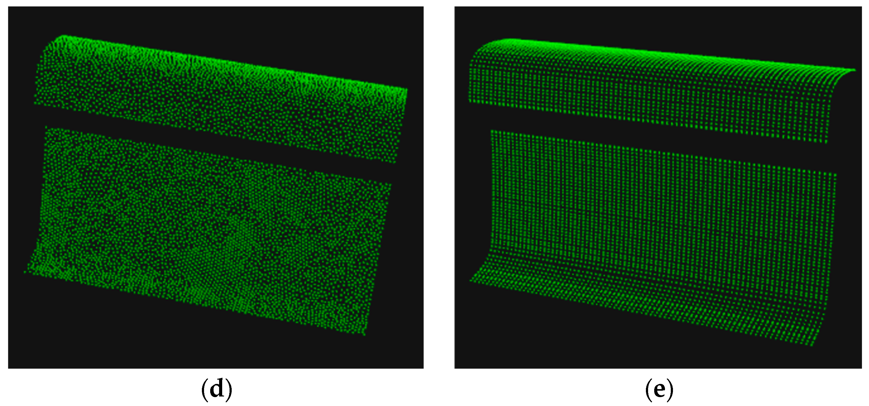
The point cloud data obtained by downsampling the point cloud still has a large amount of data, and direct point cloud calculation is not only complex but also time-consuming, which affects the speed of data processing. Therefore, representative feature points can be extracted from the source and target point clouds before point cloud alignment. This ensures that the spatial structure of the original data features remain unchanged on the premise of the extracted feature points for the later point cloud alignment work. This reduces the amount of data processed in the point cloud and improves the efficiency of point cloud alignment. Considering the geometric characteristics of point cloud data, ISS feature points are selected as the extraction method. If the point cloud set P contains n points, let pi = (xi,yi,zi), the specific process of extracting feature points is as follows:
Step 1: Establish a local coordinate system for each point pi in the point cloud set and set a search radius r for these points; determine all the points pj in the point cloud set each centered on pi and within the region of radius r. Calculate the weights wij of these points with the following expression:
w i j = 1 p i p j , | p i p j | < r
Step 2: Calculate the covariance matrix of each point pi with all the points in the neighborhood radius r:
c o v p i = | p i p j | < r w i j p i p j p i p j T | p i p j | < r w i j
Step 3: Calculate the eigenvalue of covariance matrix cov(pi) for each point pi in the point cloud set. Because the extraction of feature points has a correlation with the size of their eigenvalues, the eigenvalues are arranged in order from the largest to the smallest in order to select the feature points according to the size of the eigenvalues. Then, set the threshold ε1, ε2, take the smallest eigenvalue as the significant feature. The one that satisfies the condition of the following equation is the extracted ISS feature point, where the value of ε1, ε2 is generally less than 1.
λ i 2 λ i 1 ε 1 , λ i 3 λ i 2 ε 2

3.2. 4PCS Point Cloud Coarse Alignment

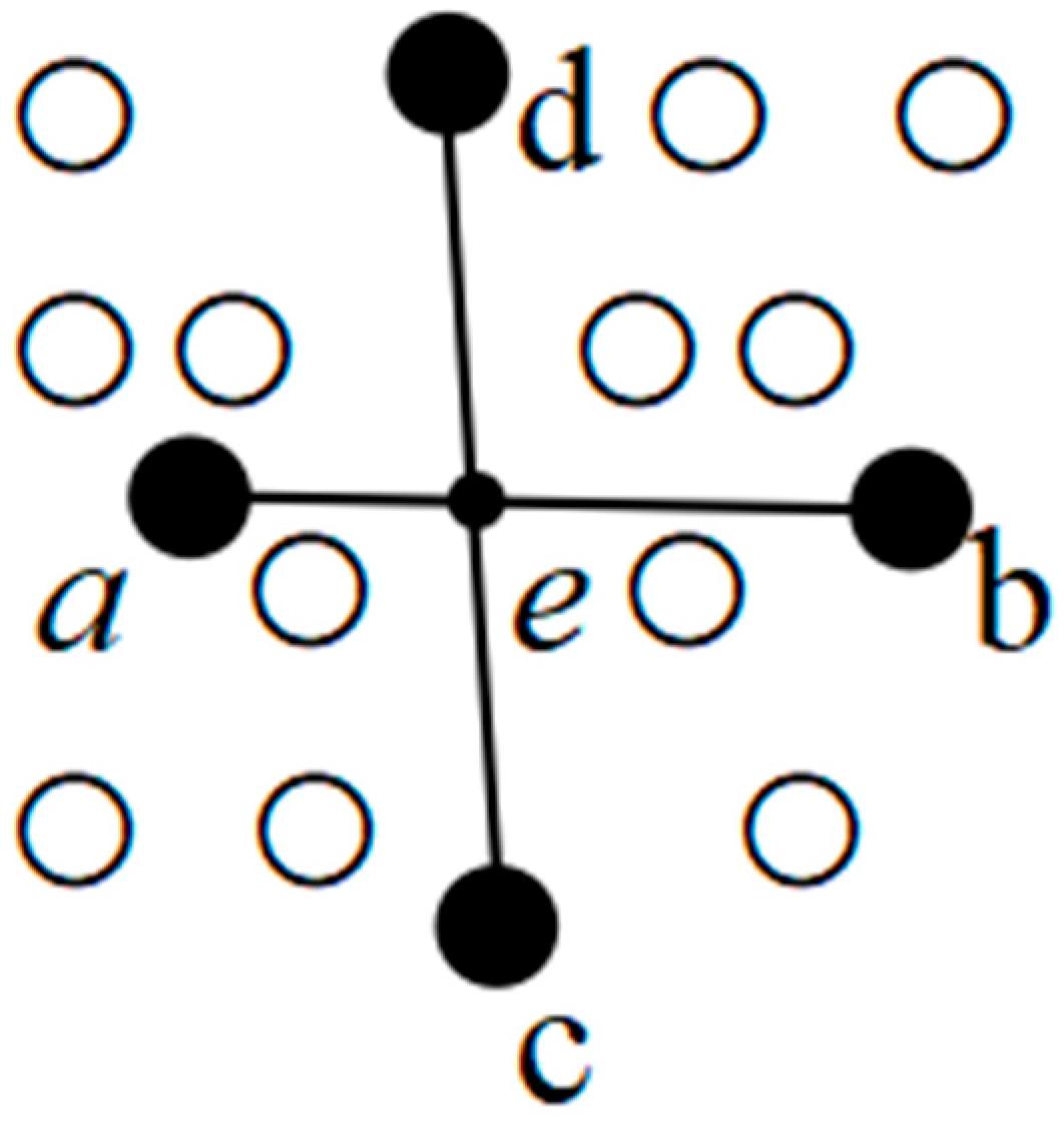
The 4PCS algorithm is a popular point cloud coarse alignment algorithm that performs a full-range search of a point cloud dataset under specified constraints. As shown in Figure 5, the basic principle of the 4PCS algorithm is as follows: randomly select 4 points (a, b, c, d) that are coplanar but not collinear in the source point cloud set P to form a point set B, where the line from ab intersects the line from cd at point e. Then, select 4 pairs of coplanar but not collinear points that are congruent with point set B from the target point cloud set Q and compute the optimal transformation matrix T.
The specific steps to implement the 4PCS algorithm are as follows:
Step 1: Four points that are coplanar and noncollinear are selected from the source point cloud set P to form a 4-point set B = {a, b, c, d}, and two affine invariant scale factors r1 and r2 are defined in this point set with the following expressions:
r 1 = a e a b
r 2 = c e c d
Step 2: Based on the calculated scale factors r1 and r2, all the point sets B’ = {a’, b’, c’, d’} that are consistent with the point set B within the permissible range are traversed from within the target point cloud set Q, and the time complexity of the algorithm is O(n2 + k) (a measure of the complexity of the execution time of the algorithm, n is the number of candidate points and k is the number of 4-point sets). Then, traverse all the point sets B’ to find the rigid body transformation matrix Ti of the point sets B and B’ using the least squares method.
Step 3: Through many iterations, the minimum distance between the source point cloud and the target point cloud after rigid-body transformation is calculated. The sum of the squares of the minimum distances is used as the optimal solution of the rigid-body transformation to realize the coarse alignment of the point cloud.

3.3. 4PCS Coarse Alignment Based on ISS Feature Points

When the 4PCS algorithm is applied to point cloud coarse alignment, due to the need to traverse all the 4-point sets from the target point cloud that have affine invariant consistency features with the source point cloud, which leads to a long time and inefficiency of the coarse alignment. To address the above problems, this paper introduces ISS feature points on the basis of 4PCS algorithm. Although the time complexity O(n2 + k) of searching for point pairs in the target point cloud remains unchanged, the number of points searched by the algorithm is reduced due to the ISS feature points extracted from the source point cloud and the target point cloud, which in turn reduces the time of coarse alignment. The coarse alignment process based on the ISS feature points is shown in Figure 6. After inputting the source and target point clouds at the same time, voxel filtering is used to downsample the source and target point clouds. Next, the ISS feature points are extracted to form the source and target point cloud feature points, and these feature points are used for 4PCS coarse alignment. Finally, the RMSE is computed and the optimal transformation matrix is output.
Step 1: Due to the large amount of data collected from the source and target point clouds, the two pieces of point clouds are downsampled first, and then the ISS algorithm is utilized to extract the feature points of the downsampled two pieces of point clouds.
Step 2: The feature points of the target point cloud are traversed by determining the coplanar disjoint 4-point set of the source point cloud feature points. The 4PCS coarse alignment is used to align the source point cloud feature points with the feature points of the target point cloud. Then, the least squares method is used to calculate the rigid-body transformation matrix of the two feature points.
Step 3: According to the derived rigid-body transformation matrix, the spatial positional transformation of the source point cloud feature points is performed. After several iterations, the sum of the nearest-point distances between the source and target point cloud feature points after the positional transformation is calculated. The rigid-body transformation matrix of the sum of the nearest-point distances will be used as the final positional transformation matrix outputted by the 4PCS algorithm between the source and target point cloud feature points.
Step 4: To analyze the error of the coarse alignment results, this paper chooses root mean square error (RMSE) as the evaluation index to measure the accuracy of the point cloud alignment. RMSE is used to quantify the size of the error of the alignment by calculating the square root of the ratio of the square sum of the distances of the matched pairs of pi and qi to the logarithmic value of n, and the smaller the value, the better the result of the alignment. The expression is as follows:
R M S E = i = 1 n p i q i 2 n

3.4. ICP Fine Alignment Based on Kd-Tree

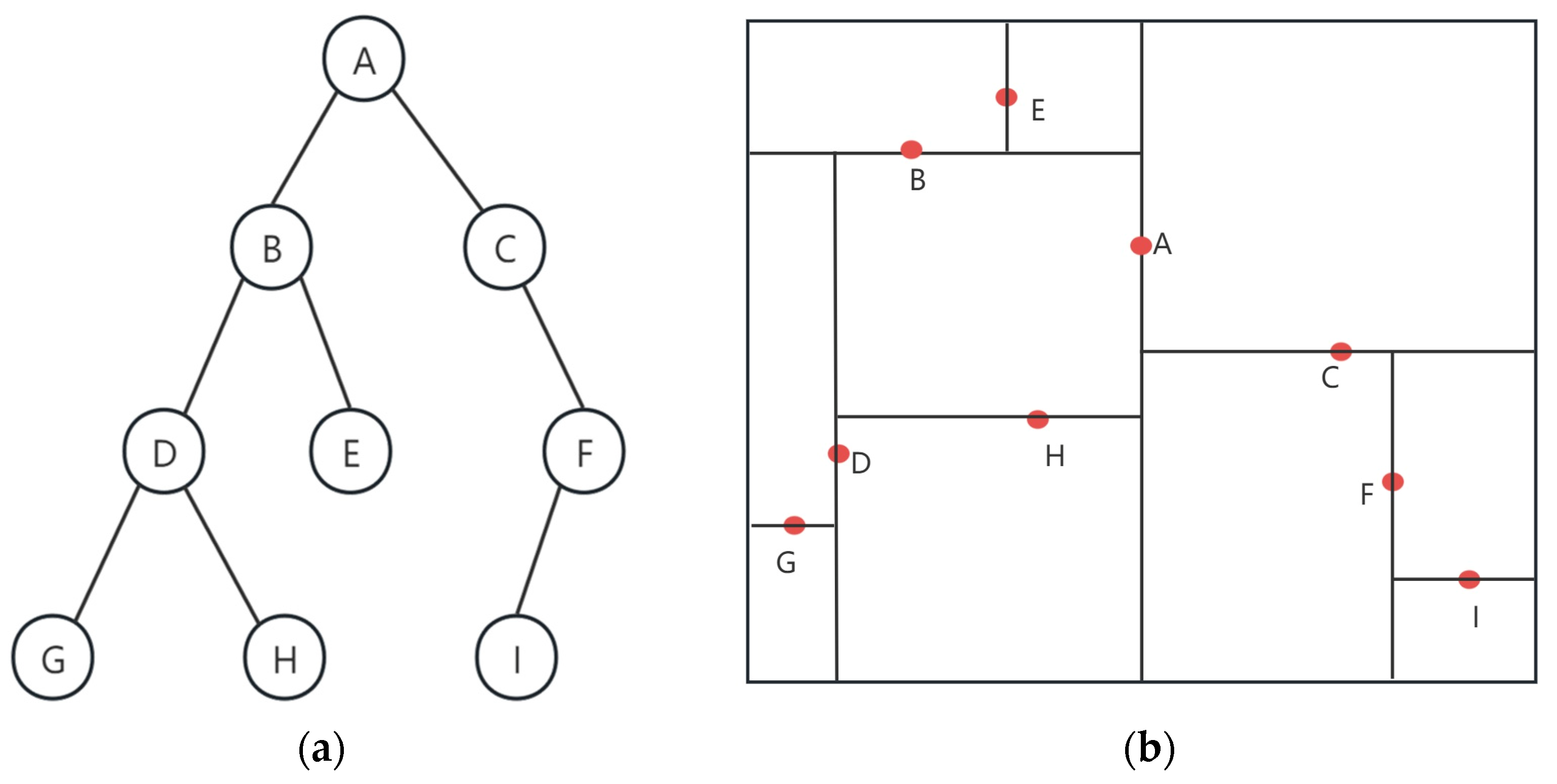
After the 4PCS coarse alignment stage, the contour between the source point cloud attitude transformation and the target point cloud can be basically overlapped. But there still exists a certain contour error, which requires fine alignment to improve the alignment accuracy. ICP is used as a classical point cloud alignment algorithm: through the matching of points to points and iteratively calculating the optimal solution of the transformation matrix of the source point cloud and the target point cloud, the alignment error is minimized. Because the ICP algorithm does not need any feature computation to achieve fast iteration to minimize the function error to get the required spatial transformation matrix, it is widely used in point cloud fine alignment. This paper adds the kd-tree on the basis of ICP to further optimize the computation time of the algorithm. kd-tree is a kind of tree data structure with a number of points in a k-dimensional space. It is widely used in range search and nearest neighbor search, as shown in Figure 7, and its basic principle is as follows:
In kd-tree, the median value of each dimension is often used as the segmentation hyperplane. The root of the tree is the first dimension, and all child nodes are divided downward by this dimension. The basis for the division is as follows: if this node is smaller than the root node, it will be divided into the left branch of the next dimension; if it is larger than the root node, it will be divided into the right branch of the next dimension. Then, the second dimension after the division is the root node, which is divided according to the above division principle and then divided downward until the end of the leaf nodes.
The traditional point-to-point ICP algorithm uses the distance between the corresponding points of two point clouds as the objective function to calculate the transformation matrix. The point-to-face ICP algorithm adopted in this paper uses the distance from each point in the source point cloud to the plane where the normal vector of the corresponding point in the target point cloud is located as the alignment criterion, and then iterates to find the optimal transformation matrix to find the best solution. The main steps of the kd-tree based point-to-plane ICP algorithm are as follows:
Step 1: In order to solve the normal features of each point in the two point cloud sets, establish a kd-tree for near-neighborhood accelerated search on the source point cloud set P and the target point cloud set Q obtained after coarse alignment. Then, compute the weighting factor and feature descriptor based on the normal features, so as to find the corresponding point of each nearest neighbor of the source point cloud set P and the target point cloud set Q.
Step 2: The optimal transformation matrix T is solved based on the found nearest neighbors with the objective function:
F R f , T f = min i = 1 N F R f , T f p i q i n i 2 N
where Rf is the rotation matrix; Tf is the translation matrix; pi and qi are the corresponding points of the source point cloud set P and the target point cloud set Q; and ni denotes the normal vector of the point pi corresponding to qi.
Step 3: Set the maximum number of iterations Nmax and the minimum threshold ε. Repeat the above steps; if the error of the two iterations is less than ε, i.e., Fn(Rf,Tf)-Fn-1(Rf,Tf) < ε, or the number of iterations is greater than Nmax, then stop iteration and find the final transformation matrix T. Otherwise, continue to iterate until it meets the iteration conditions.

4. Analysis of Experimental Results

In order to verify the feasibility of the algorithm, the experimental computer is equipped with Intel(R)Core(TM)i5-10210U@1.60GHz2.11GHz from Huawei in China (Shenzhen, China), 16G running memory, Windows 11, 64-bit operating system, and the development environment of Visual Studio2022 combined with C++ and the open-source Point Cloud Library (PCL) version 1.13.0 to realize the algorithm.

4.1. Quantitative Analysis of ISS Feature Points

When using the 4PCS algorithm based on ISS feature points for coarse alignment, the number of extracted ISS feature points affects the speed and accuracy of coarse alignment. In order to verify the feasibility and effectiveness of this algorithm, the optimal number of ISS feature points needs to be determined, and the following quantitative analysis is conducted on the effect of different numbers of ISS feature points on coarse alignment. The initial number of source point clouds is 4,137,760, and the number of target point clouds is 4,781,288. Considering that the coarse alignment involves aligning the source point clouds with the target point clouds by the positional transformation, the quantitative analysis is based on the target point clouds by increasing about 500 feature points each time to carry out nine groups of experiments. The experiments are set up with the key parameters of the ISS feature points: the radius of the spherical neighborhood of the covariance matrix and the number of feature points extracted from the source and target point clouds. The results of the coarse alignment experiments are shown in Table 2, in which the running time and the RMSE are the evaluation indexes of this quantitative analysis. The number of ISS feature points of the target point cloud extracted by setting the radius of the spherical neighborhood of the covariance matrix essentially meets the experimental requirements. It can be seen from the data in Table 2 that with the increase in the number of extracted ISS feature points, the running time of the algorithm shows a trend of increasing. On the contrary, the value of the RMSE shows a trend of decreasing, which means that the accuracy of the algorithm is continuously improved with the increase in the number of feature points.
The running effect of the 4PCS coarse alignment algorithm with different numbers of feature points is shown in Figure 8. From Figure 8a, it can be seen that when the number of ISS feature points of the target point cloud is extracted to be 996, the source and target point clouds are still in the initial spatial position, which also explains the invalidity of the RMSE values in Table 2. From Figure 8b–g, it can be seen that when the number of extracted feature points is between 1500–4000, the spatial position of the source point cloud has a tendency to be close to the target point cloud. From Figure 8g–i, it can be concluded that when the number of feature points reaches 4000–5000, the spatial position of the two point clouds essentially reaches the overlap state. This is combined with Table 2 to analyze the effect of coarse alignment for the number of points around 4000–5000. When the number of feature points is 3998, its running time is 4.59 s, and its accuracy measure RMSE value is 2.438 mm, which is 1.166 mm higher than 1.272 mm for 4998 feature points and 1.058 mm higher than 1.38 mm for 4496 feature points, and the difference is more than 1 mm. Since the higher the RMSE value, the lower the accuracy, the coarse alignment accuracy at this number of points is lower. When the number of feature points is 4496, although its accuracy measure RMSE is 0.108 mm higher than that of 4998 feature points, its running time is 6.57 s, which is 2.991 s less than that of 9.461 s for 4998 feature points. Considering the influence of the difference between the two on the running time and the accuracy on the alignment, the number of ISS feature points of the target point cloud is finally chosen to be 4496 as the amount of data used for the 4PCS coarse alignment.

4.2. Comparative Analysis of Coarse Alignment Algorithms

On the basis of 1847 and 4496 ISS feature points extracted from the source and target point clouds, the 4PCS coarse alignment method is used with PCA, SAC, K-4PCS, and the original 4PCS algorithms for coarse alignment of model 60 rails, and the resulting alignment results are shown in Figure 9.
From Figure 9b,c, it can be seen that the source and target point clouds of the PCA algorithm and SAC algorithm have obvious deviations, especially the PCA algorithm, which has the largest deviation. From Figure 9d,f, it can be seen that the 4PCS algorithm, K-4PCS algorithm, and the 4PCS algorithm based on the ISS feature points of this paper reach a basic overlap of the two point cloud models after the coarse alignment, which can provide a good initial position for the fine alignment. Table 3 shows the average values of the results obtained by the algorithm running 10 times, and the reliability of the algorithm is verified by comparing the two evaluation criteria of the algorithm’s running time and RMSE. From the data in the table, when the number of the extracted source point clouds is 1847 and the number of the target point clouds is 4496, this paper’s 4PCS algorithm based on the ISS feature points takes 1.48 s less time than the optimal K-4PCS algorithm, 1.48 s less time than the 4PCS algorithm, and 3.64 s less than the 4PCS algorithm; the alignment accuracy is improved by about 0.27 mm or so compared with these two algorithms.

4.3. Comparative Analysis of Fine Matching Algorithms

For the fine alignment stage, on the basis of 4PCS algorithm based on ISS feature points, the point cloud alignment effect of model 60 rails obtained by using the NDT algorithm, the traditional ICP algorithm, the GICP algorithm, and the KD-ICP algorithm in this paper is shown in Figure 10. From the figure, it can be seen that the four algorithms used have achieved a good overlap between the source point cloud and the target point cloud.
The average values of the results obtained by the four algorithms for 10 runs are shown in Table 4. From the data in Figure 10 and Table 4, it can be seen that the RMSE values of the four algorithms are basically the same. however, the KD-ICP algorithm in this paper is 22.309 ms in terms of runtime, which is 71.39% higher than that of the traditional ICP algorithm, 79.02% higher than that of the GICP algorithm, and 83.11% higher than that of the NDT algorithm.

4.4. Implementation of Rail Wear Calculation

For the combination of algorithms proposed in this paper, the 4PCS algorithm based on ISS feature points is used in the coarse alignment stage and the KD-ICP algorithm based on kd-tree accelerated search is used in the fine alignment stage. The combination of ISS-4PCS + KD-ICP algorithms is used for the point cloud alignment of the 60 model rails and compared and analyzed with the original 4PCS + ICP algorithms. The data obtained are shown in Table 5 and Table 6, and the effect comparison is shown in Figure 11.
As can be seen from Table 5 and Table 6 and Figure 11, the ISS-4PCS algorithm is significantly better than the original 4PCS algorithm both in terms of running time and alignment accuracy, and the KD-ICP algorithm has a great improvement over the original ICP algorithm in terms of time. The total alignment time of the 4PCS + ICP algorithm is 10.689 s and the alignment accuracy reaches 1.388 mm, while the total alignment time of the ISS-4PCS + KD-ICP algorithm is 6.592 s and the alignment accuracy reaches 1.103 mm. Overall, the ISS-4PCS + KD-ICP algorithm has an improvement of 38.33% in alignment time and 20.53% in alignment accuracy compared with the 4PCS + ICP algorithm.
In the calculation of wear on rails after fine alignment, as wear generally occurs in the inner working surface, rail section wear is mainly divided into horizontal wear ΔM and vertical wear ΔH, as shown in Figure 12, where the horizontal wear ΔM measurement position is located on the working surface of the rail head from the standard tread surface down 16 mm a position, and the vertical wear ΔH measurement position is located on the working surface of the rail head from the width of the standard tread surface b position. The total wear W is half of the vertical wear ΔH plus the horizontal wear ΔM, i.e.:
W = Δ H + 1 2 Δ M
Finally, the deviation value between the source point cloud and the target point cloud after fine alignment can be combined with the wear calculation formula to derive the rail wear value.

4.5. Experiments on Rail Wear Calculation

In order to verify the effectiveness of the ISS-4PCS + KD-ICP two-stage point cloud alignment method proposed in this paper, a 400 mm long 60 kg/m model standard railroad track is selected for this experiment. This validation process uses a quantitative test method for wear values, and a numerical test is carried out at intervals of 40 mm; the 10 sets of wear data obtained are shown in the form of Table 7.
As can be seen from Table 7, the wear values obtained using the ISS-4PCS + KD-ICP method proposed in this paper as well as a conventional measuring ruler are on the small side, which is attributed to the fact that the selected 60 kg/m model rails are freshly polished new rails, and the amount of wear itself is small. The wear errors were analyzed: the maximum error on vertical wear ΔH was 0.047 mm, that on horizontal wear ΔM was 0.048 mm, and the maximum error on total wear W was 0.058 mm. The maximum errors were all less than 0.06 mm, while the conventional wear calipers used had a reading error of 0.1 mm or less. It can be seen that the wear values measured by the ISS-4PCS + KD-ICP method used in this paper are within the permissible error range and meet the testing requirements.

5. Conclusions

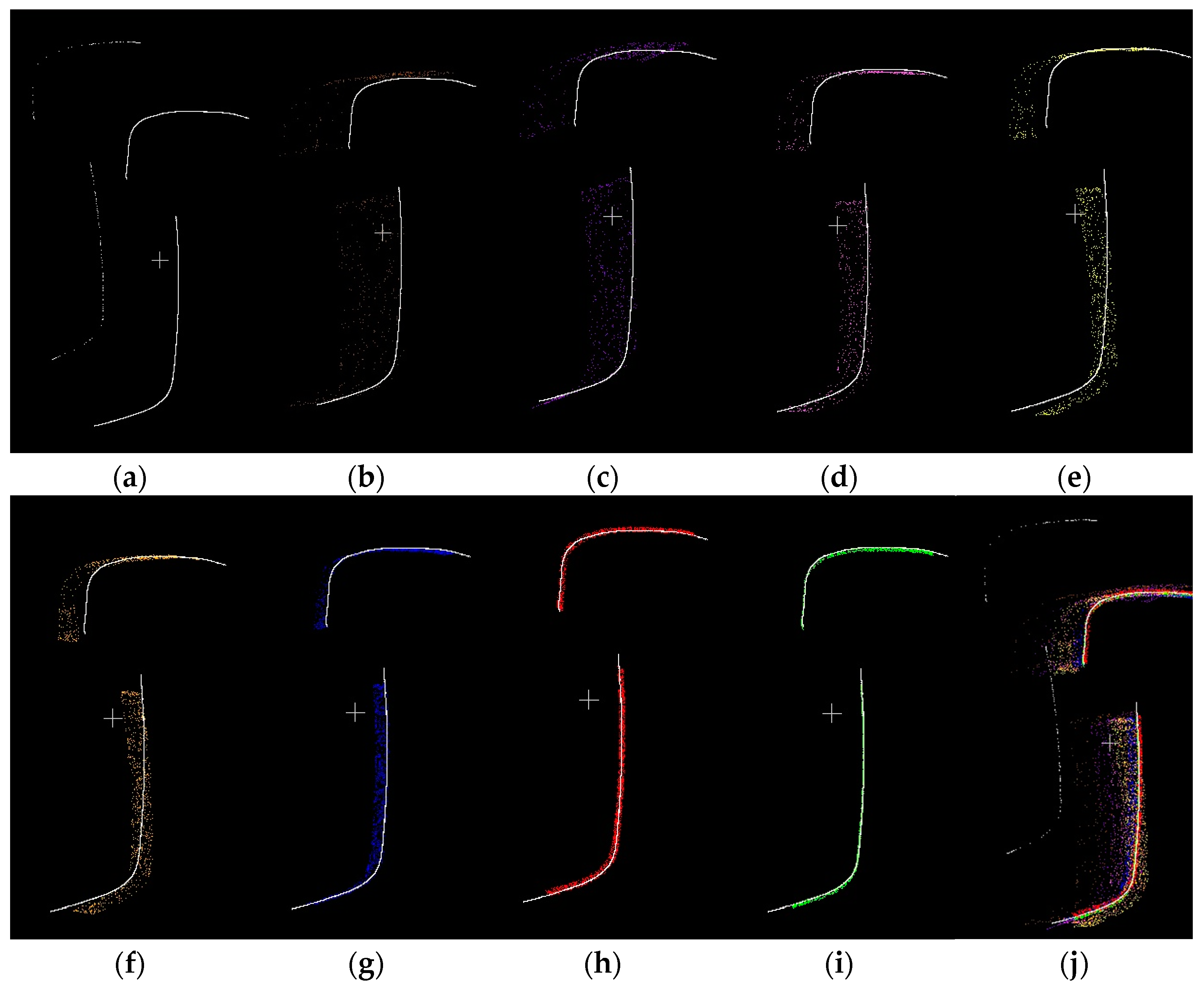
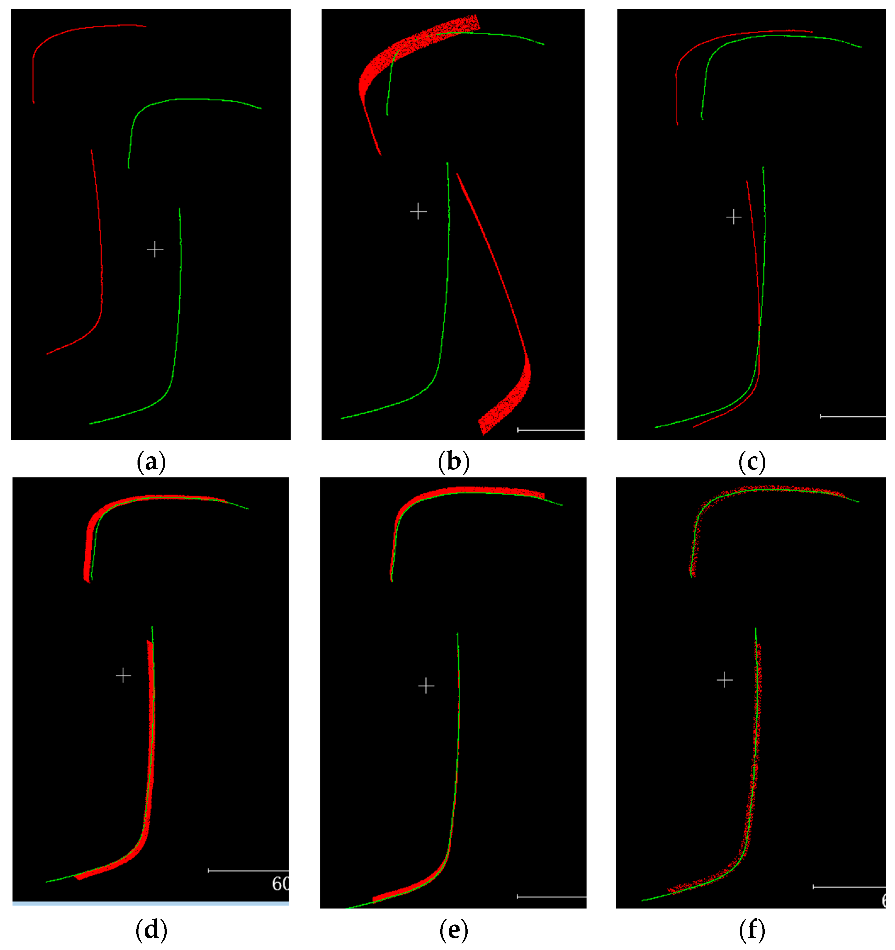
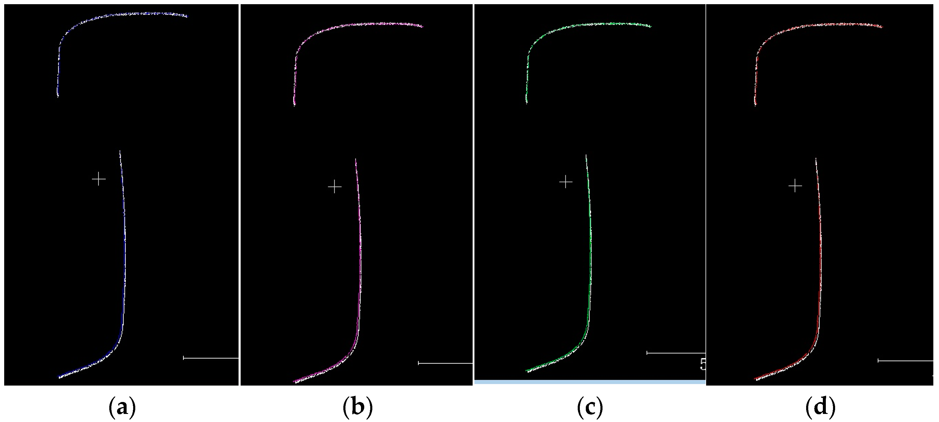
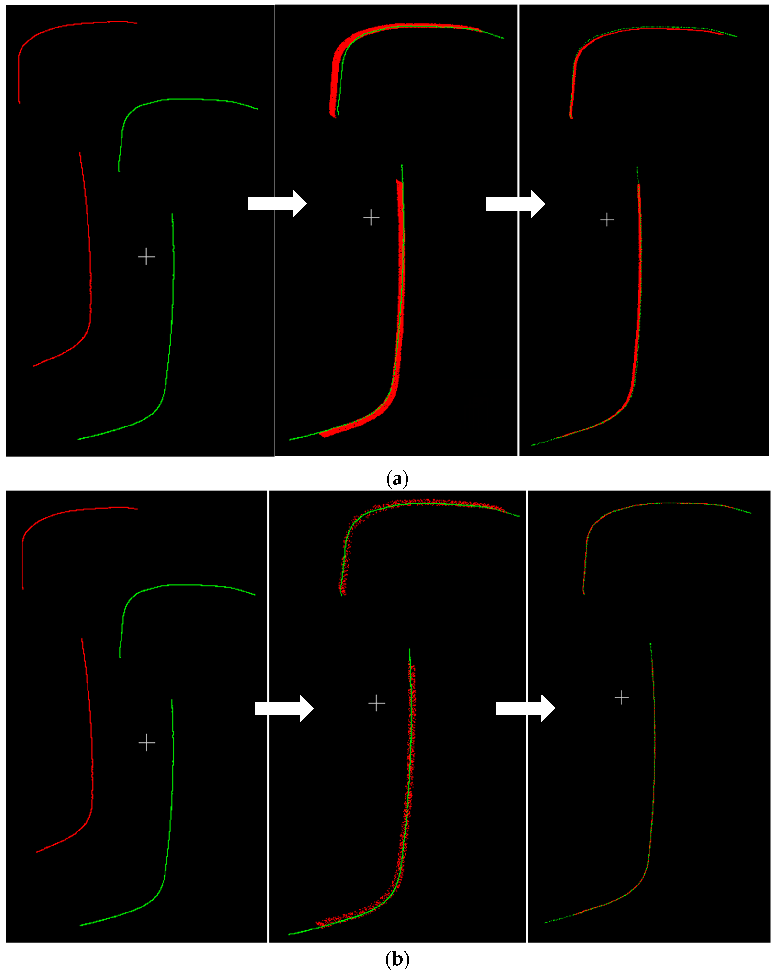
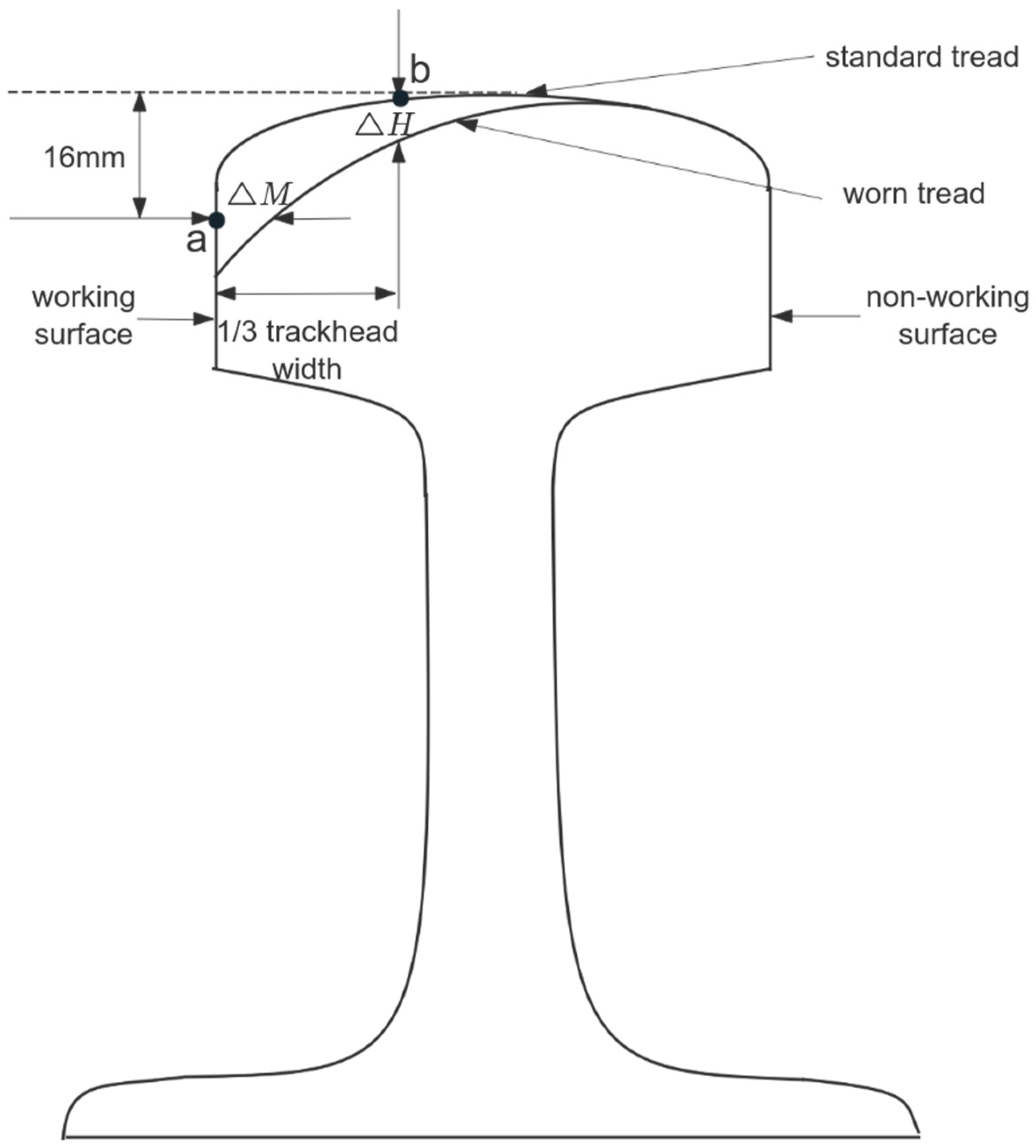
For the application of 3D line laser sensor for rail abrasion detection, a new point cloud alignment combination algorithm is proposed based on the use of voxel filtering downsampling, i.e., the combination algorithm of ISS-4PCS + KD-ICP. The experiment first downsampled the initial collected rail point cloud contour, and finally selected voxel filtering as the downsampling method for the rail point cloud contour by comprehensively considering the running time of the algorithm and the influence on the later point cloud alignment. Next, we quantitatively analyzed the extracted ISS feature points, discussed the influence of the number of extracted feature points on the coarse alignment, and determined the optimal case of the number of feature points. Considering that the proposed coarse alignment algorithm works best when the number of ISS feature points is 4496, the number of feature points of 4496 points was chosen as the number of feature points for the proposed 4PCS coarse alignment algorithm based on ISS feature points. Further, the proposed algorithm was compared and analyzed with other algorithms to verify the superiority of the proposed algorithm in terms of alignment time and accuracy. Finally, the rail vertical wear ΔH and horizontal wear ΔM were derived from the rail wear calculation experiment and then combined with the wear calculation formula to derive the total rail wear W and analyze it. The results show that the wear values measured by the ISS-4PCS + KD-ICP method used in this paper are within the permissible error range and meet the testing requirements. In the coarse alignment stage, the ISS-4PCS algorithm proposed in this paper not only improves the accuracy compared with other algorithms but also shortens the alignment time; in the fine alignment stage, although the KD-ICP algorithm used is similar to the other algorithms in terms of accuracy, it greatly shortens the alignment time and improves the efficiency of the algorithm. In general, the new method adopted in this paper shows great progress compared with the original method both in the alignment accuracy and the alignment time, which can greatly improve the detection efficiency of rail wear and provide a reference for non-contact rail wear detection methods. Although the ISS-4PCS + KD-ICP combination algorithm proposed in this paper presents better results on rail wear detection, it has not been applied on other models. Therefore, the next step is to extend the application of this combined algorithm on other models, especially on rail head geometry, in order to realize the wide range of the algorithm.

Author Contributions

Conceptualization, J.S.; methodology, J.S.; software, J.S.; writing—original draft preparation, J.S.; writing—review and editing, J.S.; supervision, H.S.; project administration, Z.N. All authors have read and agreed to the published version of the manuscript.

Funding

This research received no external funding.

Institutional Review Board Statement

Not applicable.

Informed Consent Statement

Not applicable.

Data Availability Statement

The original contributions presented in this study are included in the article. Further inquiries can be directed to the corresponding author.

Conflicts of Interest

The authors declare no conflicts of interest.

References

  1. Liu, Z.; Chen, J.; Li, W. Improved detection algorithm of rail section wear based on line structure light. Locomot. Electr. Transm. 2024, 65, 138–145. [Google Scholar] [CrossRef]
  2. Tang, K. Analysis of Track Wear Detection Method Based on Image Processing. Master’s Thesis, Shanghai University of Applied Sciences, Shanghai, China, 2021. [Google Scholar] [CrossRef]
  3. Xu, S. Measurement and Research on Track Wear Based on Surface Array CCD. Master’s Thesis, Southwest Jiaotong University, Chengdu, China, 2013. [Google Scholar]
  4. Zhu, W. Design of Railroad Track Wear Detection Terminal. Master’s Thesis, Wuhan Light Industry University, Wuhan, China, 2015. [Google Scholar]
  5. Zhao, J. Rail profile extraction and wear measurement under machine vision. Surv. Mapp. Bull. 2023, 69, 159–163+177. [Google Scholar] [CrossRef]
  6. Zuo, W.; Li, J.F.; Luo, Z.H. A fast rail profile matching algorithm based on superimposed weights ICP. Control Inf. Technol. 2023, 46, 91–97. [Google Scholar] [CrossRef]
  7. Tang, X. Research on Non-Contact Detection System of Rail Abrasion. Master’s Thesis, Southwest Jiaotong University, Chengdu, China, 2017. [Google Scholar]
  8. Liu, Y.; Bi, Y.; Zhang, L.; Huang, L. Optimization of point cloud alignment based on fusion of hyperboloid and geometric features. Laser Infrared 2024, 54, 864–869. [Google Scholar]
  9. Li, Y.; Zhang, Z.; Wang, J. RANSAC-ICP 3D point cloud alignment method based on feature point extraction. J. Shandong Univ. (Eng. Ed.) 2024, 54, 144–154. [Google Scholar]
  10. Wang, Y.; Zhang, X.; Wang, Y.; Su, H. A point cloud alignment method based on ISS-3DSC features. China Test 2025, 51, 62–67+80. Available online: http://kns.cnki.net/kcms/detail/51.1714.TB.20240126.1850.002.html (accessed on 12 December 2024).
  11. Ran, Y.; Xu, X. Point cloud registration method based on SIFT and geometry feature. Optik 2020, 203, 163902. [Google Scholar] [CrossRef]
  12. Hua, Y.N.; Liu, Y.J. Research on improved ICP algorithm based on Harris3D keypoint extraction and RANSAC algorithm. Electron. World 2021, 43, 73–74. [Google Scholar] [CrossRef]
  13. Li, R.; Yang, M.; Tian, Y.; Liu, Y.; Zhang, H. Point cloud alignment algorithm based on ISS feature points combined with improved ICP. Adv. Lasers Optoelectron. 2017, 54, 312–319. [Google Scholar]
  14. Chen, Y.; Wang, Y.; Li, J.; Liu, D.; Gao, X.; Zhang, Y. An efficient point cloud alignment algorithm based on principal component analysis. Adv. Lasers Optoelectron. 2023, 60, 376–383. [Google Scholar]
  15. Zhang, H.; Kang, G.; Zhang, Q.; Zhang, W.; Xu, W. Coarse alignment of laser point cloud based on improved SAC-IA algorithm. Aerosp. Control 2019, 37, 67–74. [Google Scholar] [CrossRef]
  16. Aiger, D.; Mitra, N.J.; Cohen-Or, D. 4-Points congruent sets for robust pairwise surface registration. ACM Trans. Graph. (TOG) 2008, 27, 85. [Google Scholar] [CrossRef]
  17. Mellado, N.; Aiger, D.; Mitra, J.N. Super 4PCS Fast Global Pointcloud Registration via Smart Indexing. Comput. Graph. Forum 2014, 33, 205–215. [Google Scholar]
  18. Theiler, W.P.; Wegner, D.J.; Schindler, K. Keypoint-based 4-Points Congruent Sets—Automated marker-less registration of laser scans. ISPRS J. Photogramm. Remote Sens. 2014, 96, 149–163. [Google Scholar]
  19. Yang, Y.; Li, J.; Wang, Y.; Yu, Y. Research on point cloud alignment algorithm based on NDT and feature point detection. Adv. Laser Optoelectron. 2022, 59, 198–204. [Google Scholar]
  20. Besl, J.P.; McKay, D.N. Method for Registration of 3-D Shapes; General Motors Research Labs.: Detroit, MI, USA, 1992. [Google Scholar]
  21. Chen, J.; Wu, X.; Wang, M.Y. 3D shape modeling using a self-developed hand-held 3D laser scanner and an efficient HT-ICP point cloud registration algorithm. Opt. Laser Technol. 2013, 45, 414–423. [Google Scholar] [CrossRef]
  22. Segal, A.; Hhnel, D.; Thrun, S. Generalized-ICP. In Proceedings of the Robotics: Science and Systems V, Seattle, WA, USA, 28 June–1 July 2009; pp. 435–442. [Google Scholar]
  23. Shen, C.; Xue, L.; Li, W.; Zheng, L.; Wu, C.; Zou, Y. A three-dimensional point cloud alignment method for robot disassembly target based on KD-ICP algorithm. Sci. Technol. Eng. 2024, 24, 9025–9032. [Google Scholar]
  24. Xiao, J.; Wang, P.; Li, W.; Li, B.; Yang, J. Application of density clustering and PCA for point cloud data processing technology in high-speed rail track inspection. Railw. Stand. Des. 2020, 64, 37–42. [Google Scholar]
Figure 1. ISS-4PCS + KD-ICP point cloud alignment method flowchart.
Applsci 15 03455 g001
Figure 2. Flow chart of 3D rail profile data acquisition.
Applsci 15 03455 g002
Figure 3. 3D point cloud data of rail profile. (a) 3D data coordinates; (b) point cloud model of rail profile.
Applsci 15 03455 g003
Figure 4. Point cloud downsampling effect. (a) Raw 3D point cloud; (b) voxel filtering; (c) stochastic filtering; (d) farthest-point filtering; (e) uniform filtering.
Applsci 15 03455 g004aApplsci 15 03455 g004b
Figure 5. 4PCS algorithm schematic. a, b, c, d are the four points chosen in P that are coplanar but not collinear; e is the intersection of the line ab with the line cd.
Applsci 15 03455 g005
Figure 6. Flowchart of 4PCS coarse alignment based on ISS feature points.
Applsci 15 03455 g006
Figure 7. kd-tree schematic. (a) Tree diagram; (b) space division diagram.
Applsci 15 03455 g007
Figure 8. The effect of coarse alignment with different number of feature points. (a) Total of 996 points; (b) total of 1502 points; (c) total of 2000 points; (d) total of 2500 points; (e) total of 3003 points; (f) total of 3497 points; (g) total of 3998 points; (h) total of 4496 points; (i) total of 4998 points; (j) comparison chart of the number of different points.
Applsci 15 03455 g008
Figure 9. Rough alignment effect. (a) Initial position before alignment; (b) PCA algorithm; (c) SAC algorithm; (d) 4PCS algorithm; (e) K-4PCS algorithm; (f) the algorithms in this paper.
Applsci 15 03455 g009
Figure 10. Precision alignment effect. (a) NDT algorithm; (b) GICP algorithm; (c) ICP algorithm; (d) KD-ICP algorithm.
Applsci 15 03455 g010
Figure 11. Comparison of rail alignment algorithms. (a) 4PCS + ICP algorithm, where the white arrow represents the direction of the alignment, and in this direction follow the initial position of the source and target point clouds before alignment, the 4PCS coarse alignment results, and the ICP fine alignment results; (b) ISS-4PCS + KD-ICP algorithm, where the white arrow represents the direction of the alignment, and in this direction follow the initial position of the source and target point clouds before alignment, the ISS-4PCS coarse alignment results, and the KD-ICP fine alignment results.
Applsci 15 03455 g011
Figure 12. Rail section wear.
Applsci 15 03455 g012
Table 1. 3D line laser sensor parameter list.
Model NumberECCO 75.200
Field of view125/190/250 mm
Measuring range250 mm
Optimum working distance325 mm
Vertical resolution12–25 μm
Horizontal resolution66–138 μm
Z linearity0.01% (0.1 μm/mm)
Z repeatability2.5 μm
Weightapprox. 480 g
Table 2. Impact of the number of feature points on coarse alignment.
Radius of Spherical Neighborhood of Covariance Matrix/mNumber of ISS EigenpointsRun Time/sRMSE/mm
Source Point Cloud Target Point Cloud
4.6051889960.124--
4.22333215020.26510.728
3.9349320000.5078.242
3.7271425001.075.865
3.5359433003 2.0214.934
3.335115234972.9463.972
3.16146039984.592.438
2.97184744966.571.38
2.822,7149989.4611.272
Table 3. Comparison of coarse alignment algorithms.
AlgorithmRun Time/sRMSE/mm
PCA 1.19.316
SAC35.583.827
4PCS10.211.655
K-4PCS8.051.648
Algorithm in this paper6.571.387
Table 4. Comparison of precision matching algorithms.
AlgorithmRun Time/msRMSE/mm
NDT 132.09131.1188
GICP106.31371.1193
ICP77.96931.1045
KD-ICP22.3091.1025
Table 5. 4PCS + ICP algorithm.
AlgorithmAlignment time/sRMSE/mm
4PCS 10.211.655
ICP0.4791.388
Table 6. ISS-4PCS + KD-ICP algorithm.
AlgorithmAlignment time/sRMSE/mm
ISS-4PCS 6.571.387
KD-ICP0.0221.103
Table 7. Calculated data for rail wear.
Point NumberVertical Wear ΔH/mmHorizontal Wear ΔM/mmTotal Wear W/mm
ISS-4PCS + KD-ICPMeasuring RulerErrorsISS-4PCS + KD-ICPMeasuring RulerErrorsISS-4PCS + KD-ICPMeasuring RulerErrors
11.2141.250.0360.8060.840.0341.6171.670.053
20.9831.030.0470.6590.670.0111.31251.3650.0525
31.1241.160.0360.7470.760.0131.49751.540.0425
41.2581.280.0220.8410.880.0391.67851.720.0415
51.2961.330.0340.8620.910.0481.7271.7850.058
61.1661.190.0240.7620.790.0281.5471.5850.038
71.0481.080.0320.6810.700.0191.38851.430.0415
81.3071.350.0430.9480.960.0121.7811.830.049
91.3921.410.0181.0051.030.0251.89451.9250.0305
101.0711.110.0390.6920.730.0381.4171.4750.058
Disclaimer/Publisher’s Note: The statements, opinions and data contained in all publications are solely those of the individual author(s) and contributor(s) and not of MDPI and/or the editor(s). MDPI and/or the editor(s) disclaim responsibility for any injury to people or property resulting from any ideas, methods, instructions or products referred to in the content.

