Prediction of Total Organic Carbon Content in Shale Based on PCA-PSO-XGBoost

Abstract

Total organic carbon (TOC) content is an important parameter for evaluating the abundance of organic matter in, and the hydrocarbon production capacity, of shale. Currently, no prediction method is applicable to all geological conditions, so exploring an efficient and accurate prediction method suitable for the study area is of great significance. In this study, for the shale of the Qingshankou Formation of the Gulong Sag in the Songliao Basin, TOC content prediction models using various machine learning algorithms are established and compared based on measured data, principal component analysis, and the particle swarm optimization algorithm. The results showed that GR, AC, DEN, CNL, LLS, and LLD are the most sensitive parameters using the Pearson correlation coefficient. The four principal components were also identified as input features through PCA processing. The XGBoost prediction model, established after selecting the parameters through PSO intelligence, had the highest accuracy with an $R^2$ and RMSE of 0.90 and 0.1545, respectively, which are superior to the values of the other models. This model is suitable for the prediction of TOC content and provides effective technical support for shale oil exploration and development in the study area.

1. Introduction

With the expansion of unconventional oil and gas exploration and development in recent years, shale oil has shown broad energy prospects and development trends [1]. Shale oil in China mainly comes from land-phase basins, with the Songliao Basin currently being a hotspot for land-phase shale oil exploration. Thick layers of dark mud shale are developed in the basin, which has the advantages of wide distribution, large reserves, and high hydrocarbon potential. The Cretaceous Qingshankou Formation shale reservoir of the Gulong Sag, which formed during the subsidence period of the Central Depression’s lake basin development, is currently the shale oil production layer with the most potential in the Songliao Basin [2,3]. Terrestrial shale oil belongs to petroleum resources aggregated within the source, and the development of shale rich in total organic carbon (TOC) content is the material basis for shale oil formation [4]. Organic matter in the Qingshankou Formation is mainly type I, and its source is mostly lacustrine stratiform algae. A total organic carbon content greater than 2% is the predicted limit of effective hydrocarbon source rock for shale oil. Therefore, the Qing 1 member can be considered a potential shale oil formation section with good oil-bearing characteristics. By contrast, the Qing 2 and Qing 3 members have hydrocarbon source rock conditions only in layers with high organic carbon content, presenting localized oil-bearing characteristics. Meanwhile, when the burial depth is shallow and the vitrinite reflectance is generally less than 0.75%, the organic matter is in the immature to low-mature stage, the hydrocarbon generation of organic matter is minimal, and the oil content in the shale is low. As the burial depth gradually increases, the vitrinite reflectance reaches 0.75~1.30%, the organic matter is in the mature stage, and a large amount of hydrocarbon is discharged. With this increase in hydrocarbon discharge, the oil content in the mud shale gradually increases [5,6,7]. In general, the depositional environment of the Qingshankou Formation provides good geological conditions for the preservation and aggregation of its organic matter.

The TOC content reflects the amount of organic matter and hydrocarbon potential in shale and is a key parameter for shale reservoir evaluation [8]. Therefore, the accurate acquisition of TOC content is indispensable in the exploration and development of shale oil. Recently, geochemical methods (e.g., Rock-Eval pyrolysis) have been used to directly determine the TOC content in coal and shale. However, in practical applications, there have been disadvantages, such as the misinterpretation of programmed pyrolysis results, the high cost of coring, and time-consuming experimental testing. Therefore, the effective use of existing data to construct predictive models has become an important means of acquisition [9,10]. Many scholars have used logging data to predict TOC content, which is mainly divided into conventional methods (∆logR method, multiple regression method, etc.) and machine learning methods [11]. Due to the complex relationship between TOC content and logging responses, machine learning methods have been widely applied in different stratigraphic and depositional environments compared to conventional methods [12]. When using machine learning methods to predict TOC content, multiple algorithms are usually established to compare and analyze the prediction results and to select the best prediction method for the study area. Wei et al. [13] established back-propagation neural networks and support vector machine prediction models by collating logging data and laboratory core analysis results after selecting logging parameters, such as natural gamma and density, as input features. Finally, the back-propagation neural network was determined to be the optimal prediction model in their comparative analysis. Tang et al. [14] established a back-propagation neural network, support vector machine, and XGBoost prediction model by selecting sensitive logging parameters of TOC content. Finally, they determined that the XGBoost prediction model performed best after conducting an accuracy check. Zhang et al. [15] predicted the TOC content of shale reservoirs based on a back-propagation neural network and a gradient-boosting decision tree algorithm using density, uranium, acoustic, and resistivity as logging parameters. Finally, they determined that the GBDT model was suitable for TOC content prediction in the study area.

In summary, the applications of the above machine learning methods are mostly limited to the algorithms themselves, and there were no in-depth analyses or processing of the logging data before establishing these models. The input variables of the model should not only have a better correlation with the target value, but the covariance between the variables should also be as low as possible for optimum performance. In addition, the proper setting of the model’s hyperparameters is very critical. For integrated learning algorithms based on boosting, when the number of weak learners, i.e., the number of decision trees, is small, the model’s fitting ability is weak, which can easily lead to underfitting. Furthermore, if the learning rate is low, it requires a more complex iteration process and greater computational volume. A larger depth of the leaf nodes will make the model more complex, allowing it to better fit the training data, but this can also easily lead to overfitting. Therefore, it is necessary to continuously adjust the combination of parameters to achieve the best prediction performance.

In this study, based on the understanding of previous researchers and the actual geological background of the study area, the correlation between the TOC content and the logging data was first quantitatively analyzed using Pearson’s correlation coefficient and heat mapping to select the sensitive parameters. Then, the selected parameters were processed using principal component analysis to determine the input features. Finally, the model parameters were optimized using the particle swarm optimization algorithm. After analyzing the errors of different models, the most suitable TOC content prediction model for the study area was determined to provide an effective basis for the exploration and development of shale oil in the study area.

2. Materials and Methods

2.1. Dataset

The research data of this study are from 8 coring wells in Qingshankou Formation, Gulong Sag, Songliao Basin, including measured TOC content and 8 logs of natural gamma (GR), natural potential (SP), shallow lateral resistivity (LLS), deep lateral resistivity (LLD), microsphere focusing resistivity (MSFL), acoustic (AC), compensated neutron (CNL), and compensated density (DEN). After data cleaning, the total sample size was 461 groups. The statistical characteristics are shown in

Table 1. Statistical characteristics of data in the study area.

	GR/API	SP/mV	LLS/(Ω·m)	LLD/(Ω·m)	MSFL/(Ω·m)	AC/(μs/m)	CNL/%	DEN/(g·cm−3)	w(TOC)/%
count	461	461	461	461	461	461	461	461	461
mean	121.59	−118.21	6.26	5.88	7.54	102.32	24.42	2.52	2.10
25%	116.51	−121.66	5.25	4.98	5.78	97.28	22.79	2.48	1.75
50%	121.63	−116.33	5.98	5.66	7.23	101.79	24.17	2.51	2.11
75%	127.13	−119.97	6.76	6.41	8.97	107.07	26.21	2.56	2.44

.

2.2. Correlation Analysis

Correlation analysis is the key to data characterization. Its main purpose is to analyze the degree of linear correlation between continuous variables and express it with statistical indicators. To more accurately describe the relationship between TOC content and logging data, quantitative correlation analysis was performed by calculating Pearson’s correlation coefficient and plotting the heat map.

Assuming that any two sets of TOC content and logging data are $X$ and $Y,$ respectively, after standardization, Pearson’s correlation coefficient value $r$ can be calculated, as shown in Equation (1). The value of $r$ ranges from −1 to 1. An absolute $r$ value closer to 1 indicates that the correlation between the two variables is higher and the correlation is better. At the same time, based on $r$, Pearson’s correlation coefficient matrix can be constructed. Then, according to the size of the color filling, the intuitive correlation heat map can be generated [16].

$$\begin{array}{c}r(X,Y)={\displaystyle \frac{\mathrm{c}\mathrm{o}\mathrm{v}(X,Y)}{\sqrt{\mathrm{v}\mathrm{a}\mathrm{r}\left(X\right)\mathrm{v}\mathrm{a}\mathrm{r}\left(Y\right)}}}\end{array}$$

(1)

where $\mathrm{c}\mathrm{o}\mathrm{v}(X,Y)$ is the covariance of $X$ and $Y$; $\mathrm{v}\mathrm{a}\mathrm{r}\left(X\right)$ and $\mathrm{v}\mathrm{a}\mathrm{r}\left(Y\right)$ are the variances of $X$ and $Y$, respectively.

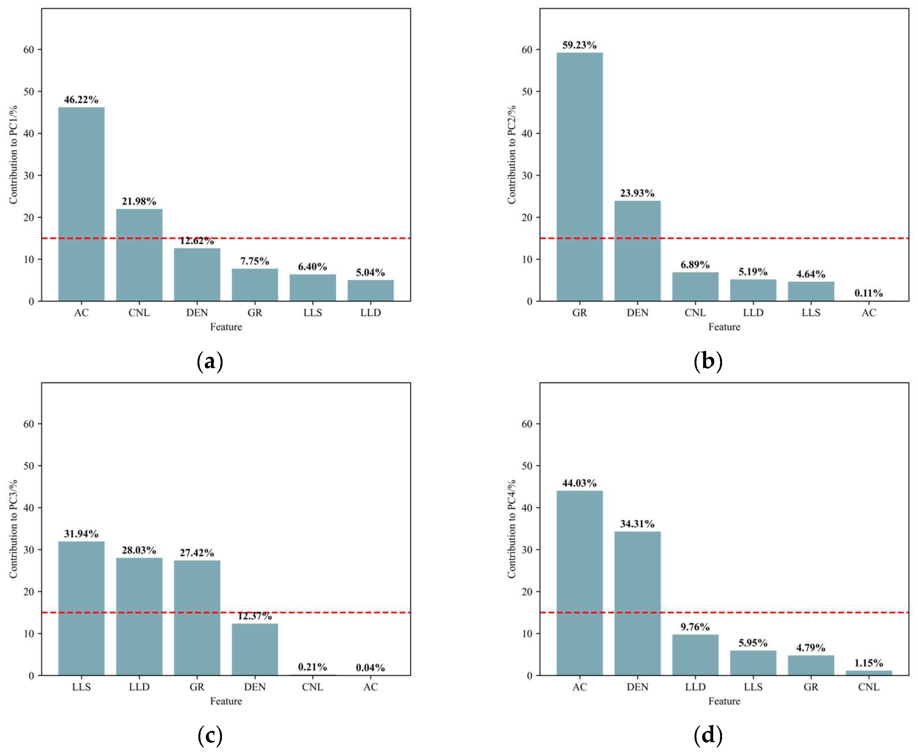
2.3. Principal Component Analysis

When there is multicollinearity in the original features, i.e., there is duplication of information between the features, they must be further processed. Principal component analysis (PCA) uses the idea of dimensionality reduction to convert a set of highly correlated independent variables into a set of variables that are independent of each other and do not have a linear relationship. The converted variables are called principal components, which reflect most of the information in the original data [17]. In applications, several principal components, which are fewer than the number of original variables and can explain most of the original data, are usually selected to replace the original variables for modeling [18].

In the principal component analysis of logging data, it is necessary to construct the original eigenmatrix $X$, as shown in Equation (2). Then, center standardization must be carried out. For simplicity, the standardized data matrix is still noted as $X$. The correlation coefficient matrix and its eigenvalues are obtained based on the cumulative contribution rate, from which the first $m$ eigenvalues are selected to build the eigenvector matrix, i.e., the matrix $Y$, as shown in Equation (3). Finally, the principal component $Z$ is calculated. As shown in Equations (4)–(6), $Z_1$ is the 1st principal component, $Z_2$ is the 2nd principal component, and $Z_m$ is the $m$th principal component.

$$\begin{array}{c}\begin{array}{c}X=\left(\begin{array}{cc}\begin{array}{ccc}{x}_{11}& x_{12}& \cdots \\ x_{21}& x_{22}& \cdots \\ ⋮& ⋮& \ddots \end{array}& \begin{array}{c}{x}_{1p}\\ x_{2p}\\ ⋮\end{array}\\ \begin{array}{ccc}{x}_{n1}& x_{n2}& \cdots \end{array}& x_{np}\end{array}\right)=(X_1,X_2,\cdots ,X_p)\end{array}\end{array}$$

(2)

where $n$ is the number of samples and $p$ is the number of logging data; $X_{np}$ is the $p$th logging value corresponding to the $n$th sample.

$$\begin{array}{c}Y=\left(\begin{array}{cc}\begin{array}{ccc}{y}_{11}& y_{12}& \cdots \\ y_{21}& y_{22}& \cdots \\ ⋮& ⋮& \ddots \end{array}& \begin{array}{c}{y}_{1m}\\ y_{2m}\\ ⋮\end{array}\\ \begin{array}{ccc}{y}_{p1}& y_{p2}& \cdots \end{array}& y_{pm}\end{array}\right)\end{array}$$

(3)

where $m$ is the number of principal components.

$$Z_1=y_{11}{X}_1+y_{21}{X}_2+{\cdots +y}_{p1}{X}_p$$

(4)

$$Z_2=y_{12}{X}_1+y_{22}{X}_2+{\cdots +y}_{p2}{X}_p$$

(5)

$$Z_m=y_{1m}{X}_1+y_{2m}{X}_2+{\cdots +y}_{pm}{X}_p$$

(6)

2.4. Particle Swarm Optimization

When using machine learning algorithms for modeling, the selection of model hyperparameters affects prediction results. The principle of hyperparameter selection is mainly judged by evaluation indexes. Only by setting the appropriate values can we achieve better evaluation results. When using different machine learning algorithms to predict TOC content, each algorithm must set hyperparameters. The problem of selecting algorithmic parameters is transformed into an optimization problem due to the difficulty of finding the optimal solution via conventional manual parameter tuning. The intelligent preferential selection of the best hyperparameters of the model is realized by particle swarm optimization.

The Particle Swarm Optimization (PSO) algorithm is a population-based metaheuristic optimization technique inspired by the collective intelligence of bird flocking or fish schooling. Each particle in the algorithm represents a potential solution in the solution space. The particles adjust their positions and speeds according to their own optimal positions (individual optimal) and the optimal positions of the flock (global optimal), gradually approaching the global optimal solution [19,20]. In constructing the TOC content prediction model, the evaluation index of the model was set as the objective function. The optimal hyperparameters of the model were determined by continuously updating the particle velocity and position. The process is shown in Equations (7) and (8).

$$v_i^{t+1}=w{v}_i^t+c_1{r}_1(p_{i,pbest}^t-x_i^t)+c_2{r}_2(p_{gbest}^t-x_i^t)$$

(7)

$$x_i^{t+1}=x_i^t+v_i^{t+1}$$

(8)

where, $v_i^{t+1}$ is the velocity of the particle in $t+1$ iterations; $v_i^t$ is the velocity of the particle in $t$ iterations; $x_i^t$ is the position of the particle in $t$ iterations; $w$ is the weight; $c_1$ is the learning factor of the individual; $c_2$ is the learning factor of the group; $r_1$ and $r_2$ are random numbers with values ranging from 0 to 1; $p_{i,pbest}^t$ is the individual optimal position of the particle in $t$ iterations; $p_{gbest}^t$ is the global optimal position in $t$ iterations.

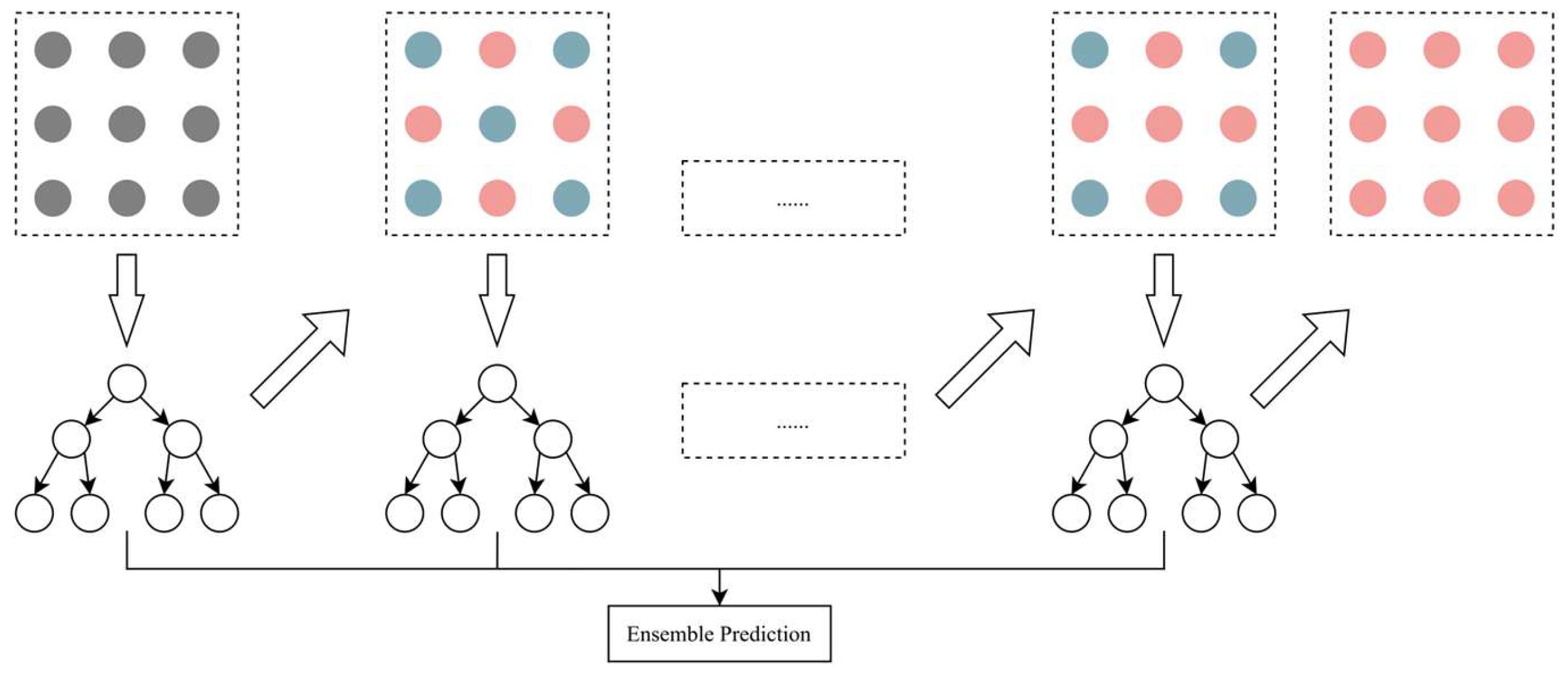
2.5. Machine Learning

2.5.1. BPNN

The BP (Back Propagation) neural network is a type of feed-forward network consisting of multiple layers, with each layer connected sequentially and information passed forward through these layers. It is one of the most widely applied neural network algorithms. The BP neural network consists of an input layer, one or more hidden layers, and an output layer. The training process involves two main phases: forward propagation of signals and backward propagation of errors. During forward propagation, input signals are processed through the hidden layers and transmitted to the output layer. If the output layer does not produce the desired output, the process shifts to the backward propagation of errors. In this phase, the network weights and thresholds are continuously updated based on the prediction error, aiming to minimize the error function [21].

The TOC content prediction model based on the BP neural network can be expressed as Equation (9).

$$y_{pre}=f(w_2·f(w_{1}x+b_1)+b_2)$$

(9)

where, $y_{pre}$ is the predicted value of TOC content; $x$ is the principal component of the log after processing; $f$ is the activation function; $w_1$ is the weight between the input layer and the hidden layer; $b_1$ is the threshold between the input layer and the hidden layer; $w_2$ is the weight between the hidden layer and the output layer; $b_2$ is the threshold between the hidden layer and the output layer.

2.5.2. GBDT

GBDT (Gradient-Boosting Decision Tree) is a gradient drop algorithm based on the CART regression tree and function space, which has the advantages of strong prediction ability and good stability. The basic principle of GBDT includes two core algorithm ideas. One is additive enhancement, and the other is gradient enhancement. The basic idea of additive enhancement is that multiple weak learners can form a stronger learner, while the basic idea of gradient enhancement is that every time a weak learner is selected, the direction of the loss function decreases the fastest, thus accelerating the convergence process [22]. GBDT builds multiple weak learners by optimizing the loss function step by step. Each new weak learner further enhances the model’s performance by fitting the residual of the current model and then obtaining the optimal model.

The TOC content prediction model based on GBDT can be expressed as Equation (10).

$$y_{pre}=F_0(x)+\sum _{k=1}^K\alpha F_k(x)$$

(10)

where, $y_{pre}$ is the predicted value of TOC content; $x$ is the principal component of the log after processing; $F_0\left(x\right)$ is the initial model; $K$ is the number of trees; $\alpha$ is the learning rate; $F_k\left(x\right)$ is the $k$th tree.

2.5.3. XGBoost

XGBoost (eXtreme Gradient Boosting) is an optimized gradient-boosting decision tree algorithm that has undergone a number of improvements, including second-order Taylor expansion of loss functions, the addition of regular terms, parallel computation, and missing value processing, which improves training speed and model generalization ability [23,24]. The XGBoost model structure is shown in Figure 1. XGBoost builds the model step by step by optimizing the objective function, which is the weighted sum of the loss function that measures the error between the predicted and true values as well as the regularization term, which controls the complexity of the model and prevents overfitting.

The TOC content prediction model based on XGBoost can be expressed as Equation (11).

$$y_{pre}=\sum _{k=1}^K{f}_k\left(x\right)$$

(11)

where, $y_{pre}$ is the predicted value of TOC content; $x$ is the principal component of the log after processing; $K$ is the number of trees; $f_k\left(x\right)$ is the $k$th tree.

2.6. Evaluation Metrics

Different tasks require different evaluation indexes to measure the model effect. The main role of evaluation indexes for the regression task is to quantify the degree of fit and error between the model prediction results and the real values, which helps assess and compare the performance of different models. In this study, the coefficient of determination ($R^2$) and Root Mean Square Error (RMSE) were used to evaluate the TOC content prediction model, as shown in Equations (12) and (13). A value of $R^2$ closer to 1 and a smaller RMSE value indicate the better fitting effect of the established TOC content prediction model.

$$R^2=1-{\displaystyle \frac{{\sum }_{i=1}^n{\left(y_i-\widehat{y_i}\right)}^2}{{\sum }_{i=1}^n{\left(y_i-\overline{y}\right)}^2}}$$

(12)

$$\mathrm{R}\mathrm{M}\mathrm{S}\mathrm{E}=\sqrt{{\displaystyle \frac{1}{n}}\sum _{i=1}^n{\left(y_i-\widehat{y_i}\right)}^2}$$

(13)

where $y_i$ is the actual value of TOC content; $\overline{y}$ is the actual mean value of TOC content; $\widehat{y_i}$ is the predicted value of TOC content; $n$ is the number of samples.

3. Results and Discussion

3.1. Logging Parameter Analysis

In building the prediction model, TOC content cannot be accurately predicted by a single logging parameter or all logging parameters; hence, sensitive logging parameters must be selected as input variables. After data normalization, the sensitive characteristics of total organic carbon content were analyzed based on Pearson’s correlation coefficient and heat maps. The results are shown in Figure 2 and Figure 3. The results show that w(TOC) is highly correlated with natural gamma (GR) and acoustic (AC), followed by compensated density (DEN), compensated neutron (CNL), shallow lateral resistivity (LLS) and deep lateral resistivity (LLD), low correlation with microsphere focusing resistivity (MSFL), and natural potential (SP). Therefore, GR, AC, DEN, CNL, LLS, and LLD logging parameters were selected as input variables for the TOC content prediction model. In addition, there is a multiple covariance relationship between logging parameters, such as compensated density (DEN) and acoustic (AC), compensated neutron (CNL) and compensated density (DEN), and shallow lateral resistivity (LLS) and deep lateral resistivity (LLD), which have high similarity and need further processing.

3.2. Logging Response Characterization

After selecting the logging parameters, PCA was used to eliminate the more complex covariance relationship between the logging data, which obtained the principal component results, as shown in Figure 4 and Figure 5. According to the analysis, the cumulative contribution rate of the first four principal components (PC) reached 95.37%, i.e., PC1, PC2, PC3, and PC4 contain more than 95% of the information in the original data. Furthermore, PC1 mainly reflects the characteristics of acoustic (AC) and compensated neutrons (CNL). PC2 mainly reflects the characteristics of natural gamma (GR) and compensated density (DEN). PC3 reflects the characteristics of shallow lateral resistivity (LLS) and deep lateral resistivity (LLD). PC4 reflects the characteristics of acoustic (AC) and compensation density (DEN). Therefore, according to the principle that the cumulative contribution rate is greater than 90%, the first four principal components were selected as new input variables to build the TOC content prediction model.

3.3. Build Prediction Model

The 461 sets of sample data in the study area were divided by 70% and 30% into a training dataset and a test dataset, respectively. The TOC content prediction model based on BPNN, GBDT, and XGBoost algorithms was established by treating the results of PCA as input values and the TOC content of core analysis as output values. The implementation process is shown in Figure 6. Due to the hyperparameters of each model requiring adjustment, and the adjustment process being speculative, the PSO algorithm and fivefold cross-validation were adopted to determine the best combination of hyperparameters for different models to reduce randomness in the selection process, avoid overfitting, and enhance prediction performance. The results of setting model hyperparameters are shown in

Table 2. Hyperparameter settings of different models.

Model	Hyperparameters	The Concept of Hyperparameters	Settings
BPNN	hidden_layer_sizes	The ith element represents the number of neurons in the ith hidden layer	(64, 64, 32)
	activation_function	Activation function for the hidden layer	$Relu$
GBDT	learning_rate	Weight reduction factor for weak learners	0.07
	n_estimators	The number of iterations for weak learners	190
	min_samples_split	The minimum number of samples required to split internal nodes	2
	min_samples_leaf	The minimum number of samples on leaf nodes	1
	max_depth	The maximum depth of tree	4
XGBoost	learning_rate	Weight reduction factor for weak learners	0.08
	n_estimators	The number of iterations for weak learners	180
	subsample	Ratio of subsampling	0.7
	colsample_bytree	Controls the sampling scale of the number of columns in the tree	0.6
	max_depth	The maximum depth of tree	5

. The BPNN prediction model consists of one input layer, three hidden layers, and one output layer. The hidden layer structure is (64, 64, 32), and the activation function is the $Relu$ function. In the GBDT and XGboost prediction models, the weak learners amount to 190 and 180, the learning rate is 0.07 and 0.08, and the maximum depth of the decision tree is 4 and 5.

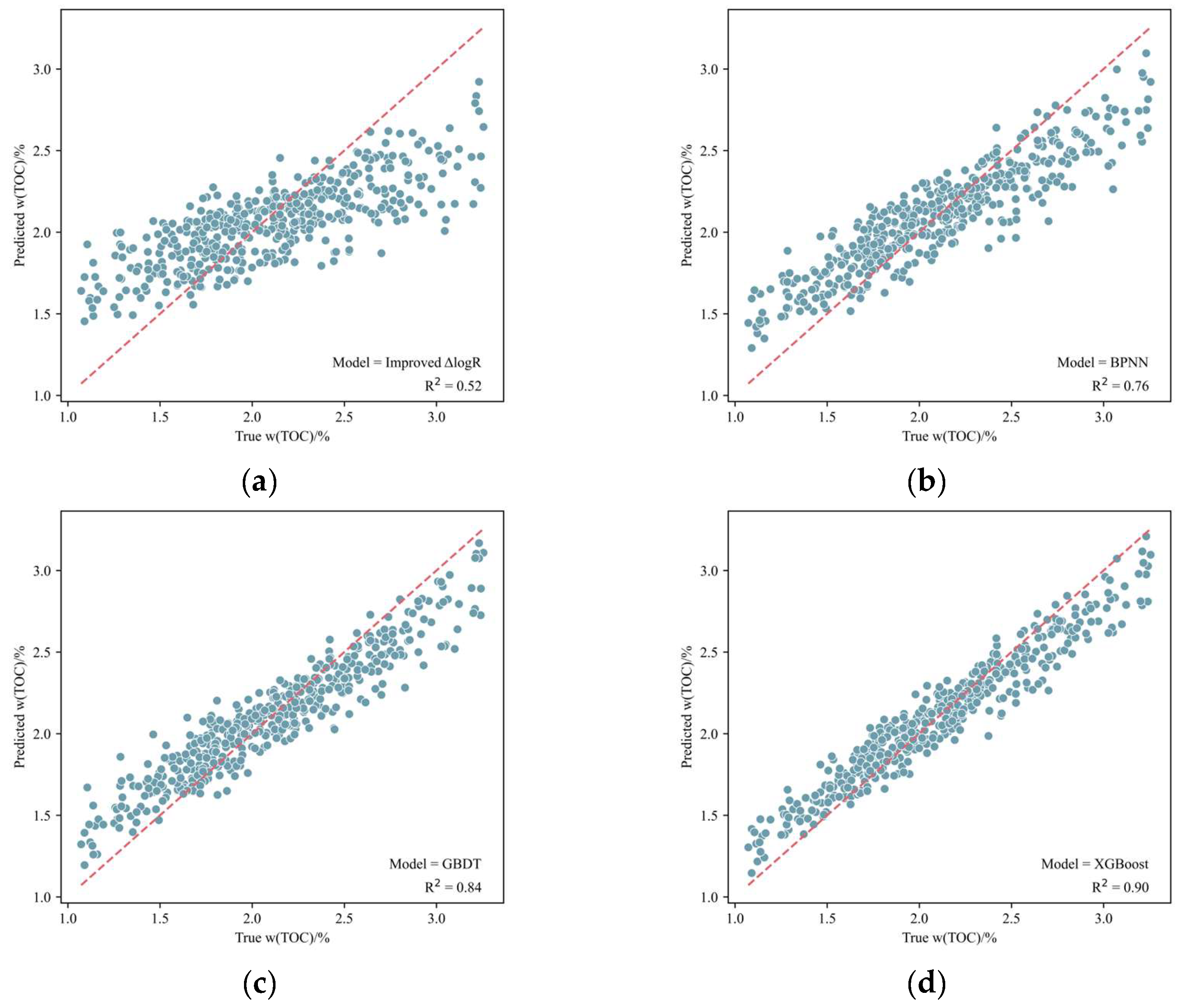
3.4. Comparative Analysis of Different Models

To further illustrate the prediction effect of machine learning methods, an improved ∆logR method was established for comparison [25]. The results are shown in Figure 7 and Figure 8. In all datasets, the XGBoost prediction model has the highest accuracy with an $R^2$ of 0.90 and RMSE of 0.1545, followed by the GBDT and BP neural network prediction models, with an $R^2$ of 0.84 and 0.76, and an RMSE of 0.1956 and 0.2375, respectively. The improved ∆logR method has the lowest accuracy with an $R^2$ of 0.52 and an RMSE of 0.3397. The $R^2$ values of different methods show significant variability. The superior performance of XGBoost stems from its ensemble learning architecture, which combines gradient-boosted decision trees with regularization, effectively capturing complex nonlinear relationships while preventing overfitting. The relatively lower $R^2$ values of the GBDT and BP neural network models reflect their respective limitations. GBDT lacks the built-in regularization of XGBoost, while the neural network’s performance is constrained by the size and architectural complexity of the dataset. The improved ∆logR method’s substantially lower $R^2$ value underscores the limitations of conventional petrophysical approaches in modeling complex reservoir relationships compared to machine learning algorithms. Furthermore, in this study, the XGBoost prediction model also outperformed other models on the training set and test set, with an $R^2$ of 0.92 and 0.88 and an RMSE of 0.1417 and 0.1598, respectively. The consistency between training and testing also confirms the XGBoost model’s excellent performance.

3.5. Comparative Analysis of Model Application

To test the application effect of the TOC content prediction model, the TOC content of the shale reservoir in the study area’s X2 well was predicted. The application results are shown in Figure 9. A low degree of conformity was observed between the predicted value and the measured value with the worst performance. The predicted value of the BP neural network prediction model was low at 2335–2345 m. The predicted value was close to the measured value at 2345–2355 m. The overall trend of GBDT and XGBoost prediction models was the same, but the predicted value of the former was lower at 2335–2355 m, while the predicted value of the latter was closer to the measured value. In summary, the XGBoost prediction model was the most effective and suitable for predicting TOC content in the study area.

4. Conclusions

In this study, based on Pearson’s correlation coefficient and heat maps, the correlation between total organic carbon content and logging data in the study area was quantitatively analyzed. GR, AC, DEN, CNL, LLS, and LLD were selected as sensitive logging responses. Principal component analysis was used to reduce collinearity between logging data, and four principal components from PC-1 to -4 were determined as input features of the model.

The prediction models of total organic carbon content based on the BP neural network, GBDT, and XGBoost algorithms were established. Optimal parameter combinations of different models were selected using the particle swarm optimization algorithm. Through comparison and analysis with conventional prediction methods, the XGBoost model was selected as the optimal prediction model for its superior performance on different datasets. Its evaluation metrics also outperformed GBDT, BP neural network, and the ∆logR improved method. It is suitable for predicting total organic carbon content in shale reservoirs in the study area.

The TOC content prediction model established using multiple methods has broad application prospects, is low cost, has strong operability, and has a high reference value for guiding significance for the prediction of TOC content in shale reservoirs in the study area.

References

1. Liu, G. Challenges and Countermeasures of Log Evaluation in Unconventional Petroleum Exploration and Development. Pet. Explor. Dev. 2021, 48, 1033–1047. [Google Scholar] [CrossRef]
2. Gao, B.; Feng, Z.; Luo, J.; Shao, H.; Bai, Y.; Wang, J.; Zhang, Y.; Wang, Y.; Yan, M. Geochemical Characteristics of Mature to High-Maturity Shale Resources, Occurrence State of Shale Oil, and Sweet Spot Evaluation in the Qingshankou Formation, Gulong Sag, Songliao Basin. Energies 2024, 17, 2877. [Google Scholar] [CrossRef]
3. Zhou, B.; Xiao, Y.; Lei, Z.; Wang, R.; Hu, S.; Hou, X. Controlling Factors for Oil Production in Continental Shales: A Case Study of Cretaceous Qingshankou Formation in Songliao Basin. Pet. Res. 2023, 8, 183–191. [Google Scholar] [CrossRef]
4. He, W.; Sun, N.; Zhang, J.; Zhong, J.; Gao, J.; Sheng, P. Genetic Mechanism and Petroleum Geological Significance of Calcite Veins in Organic-Rich Shales of Lacustrine Basin: A Case Study of Cretaceous Qingshankou Formation in Songliao Basin, China. Pet. Explor. Dev. 2024, 51, 1083–1096. [Google Scholar] [CrossRef]
5. Zhang, S.; Zhang, B.; Wang, X.; Feng, Z.; He, K.; Wang, H.; Fu, X.; Liu, Y.; Yang, C. Gulong Shale Oil Enrichment Mechanism and Orderly Distribution of Conventional– Unconventional Oils in the Cretaceous Qingshankou Formation, Songliao Basin, NE China. Pet. Explor. Dev. 2023, 50, 1045–1059. [Google Scholar] [CrossRef]
6. Huang, Y.; Zhang, J.; Zhang, S.; Wang, X.; He, K.; Guan, P.; Zhang, H.; Zhang, B.; Wang, H. Petroleum Retention, Intraformational Migration and Segmented Accumulation within the Organic-Rich Shale in the Cretaceous Qingshankou Formation of the Gulong Sag, Songliao Basin, Northeast China. Acta Geol. Sin.-Engl. Ed. 2023, 97, 1568–1586. [Google Scholar] [CrossRef]
7. Liu, B.; Wang, L.; Fu, X.; Huo, Q.; Bai, L.; Lyu, J.; Wang, B. Identification, Evolution and Geological Indications of Solid Bitumen in Shales: A Case Study of the First Member of Cretaceous Qingshankou Formation in Songliao Basin, NE China. Pet. Explor. Dev. 2023, 50, 1345–1357. [Google Scholar] [CrossRef]
8. Chen, S.; Wang, X.; Li, X.; Sui, J.; Yang, Y.; Yang, Q.; Li, Y.; Dai, C. Geophysical Prediction Technology for Sweet Spots of Continental Shale Oil: A Case Study of the Lianggaoshan Formation, Sichuan Basin, China. Fuel 2024, 365, 131146. [Google Scholar] [CrossRef]
9. Zou, W. Artificial Intelligence Research Status and Applications in Well Logging. Well Logging Technol. 2020, 44, 323–328. [Google Scholar] [CrossRef]
10. Hazra, B.; Dutta, S.; Kumar, S. TOC Calculation of Organic Matter Rich Sediments Using Rock-Eval Pyrolysis: Critical Consideration and Insights. Int. J. Coal Geol. 2017, 169, 106–115. [Google Scholar] [CrossRef]
11. Wang, J.; Xu, Y.; Sun, P.; Liu, Z.; Zhang, J.; Meng, Q.; Zhang, P.; Tang, B. Prediction of Organic Carbon Content in Oil Shale Based on Logging: A Case Study in the Songliao Basin, Northeast China. Geomech. Geophys. Geo-Energy Geo-Resour. 2022, 8, 44. [Google Scholar] [CrossRef]
12. Lai, J.; Bai, T.; Su, Y.; Zhao, F.; Li, L.; Li, Y.; Li, H.; Wang, G.; Xiao, C. Researches progress in well log recognition and evaluation of source rocks. Geol. Rev. 2024, 70, 721–741. [Google Scholar] [CrossRef]
13. Wei, M.; Zhou, J.; Duan, Y. Prediction Model of Total Organic Carbon Content in Shale Gas. Sci. Technol. Eng. 2023, 23, 12917–12925. [Google Scholar] [CrossRef]
14. Tang, S.; Yang, B.; Jin, J.; Liu, H.; Dai, X.; Pu, J. Comparative Study on Total Organic Carbon Content Logging Prediction Method Based on Machine Learning. Well Logging Technol. 2024, 48, 428–437. [Google Scholar] [CrossRef]
15. Zhang, Y.; Zhang, G.; Zhao, W.; Zhou, J.; Li, K.; Cheng, Z. Total Organic Carbon Content Estimation for Mixed Shale Using Xgboost Method and Implication for Shale Oil Exploration. Sci. Rep. 2024, 14, 20860. [Google Scholar] [CrossRef]
16. Cheng, B.; Xu, T.; Luo, S.; Chen, T.; Li, Y.; Tang, J. Method and Practice of Deep Favorable Shale Reservoirs Prediction Based on Machine Learning. Pet. Explor. Dev. 2022, 49, 1056–1068. [Google Scholar] [CrossRef]
17. Zhang, Y.; Wang, G.; Wang, X.; Fan, H.; Shen, B.; Sun, K. TOC Estimation from Logging Data Using Principal Component Analysis. Energy Geosci. 2023, 4, 100197. [Google Scholar] [CrossRef]
18. Chen, D.; Huang, C.; Wei, M. Shale Gas Production Prediction Based on PCA-PSO-LSTM Combination Model. J. Circuits Syst. Comput. 2024, 33, 2450176. [Google Scholar] [CrossRef]
19. Ahangari, D.; Daneshfar, R.; Zakeri, M.; Ashoori, S.; Soulgani, B.S. On the Prediction of Geochemical Parameters (TOC, S1 and S2) by Considering Well Log Parameters Using ANFIS and LSSVM Strategies. Petroleum 2022, 8, 174–184. [Google Scholar] [CrossRef]
20. Lu, C.; Jiang, H.; Yang, J.; Wang, Z.; Zhang, M.; Li, J. Shale Oil Production Prediction and Fracturing Optimization Based on Machine Learning. J. Pet. Sci. Eng. 2022, 217, 110900. [Google Scholar] [CrossRef]
21. Liu, D. Prediction Method of TOC Content in Mudstone Based on Artificial Neural Network. IOP Conf. Ser. Earth Environ. Sci. 2021, 781, 022087. [Google Scholar] [CrossRef]
22. Qian, S.; Dong, Z.; Shi, Q.; Guo, W.; Zhang, X.; Liu, Z.; Wang, L.; Wu, L.; Zhang, T.; Li, W. Optimization of Shale Gas Fracturing Parameters Based on Artificial Intelligence Algorithm. Artif. Intell. Geosci. 2023, 4, 95–110. [Google Scholar] [CrossRef]
23. Hou, M.; Xiao, Y.; Lei, Z.; Yang, Z.; Lou, Y.; Liu, Y. Machine Learning Algorithms for Lithofacies Classification of the Gulong Shale from the Songliao Basin, China. Energies 2023, 16, 2581. [Google Scholar] [CrossRef]
24. Sun, J.; Dang, W.; Wang, F.; Nie, H.; Wei, X.; Li, P.; Zhang, S.; Feng, Y.; Li, F. Prediction of TOC Content in Organic-Rich Shale Using Machine Learning Algorithms: Comparative Study of Random Forest, Support Vector Machine, and XGBoost. Energies 2023, 16, 4159. [Google Scholar] [CrossRef]
25. Liu, C.; Zhao, W.; Sun, L.; Zhang, Y.; Chen, X.; Li, J. An Improved ΔlogR Model for Evaluating Organic Matter Abundance. J. Pet. Sci. Eng. 2021, 206, 109016. [Google Scholar] [CrossRef]
Figure 1. XGBoost model structure.
Applsci 15 03447 g001
Figure 2. Logging parameters and total organic carbon content correlation.
Applsci 15 03447 g002
Figure 3. Sensitive parameter ranking of total organic carbon content.
Applsci 15 03447 g003
Figure 4. Principal component analysis gravel diagram. The contribution rate of PC1 is the highest at 51.98%. The contribution rate of PC2 is 14.96%. The contribution rate of PC3 is 7.47%. The contribution rate of PC4 is 4.72%. The contribution rates of PC5 and PC6 are 1.91% and 0.48%, respectively.
Applsci 15 03447 g004
Figure 5. Ranking of feature contributions to principal components. (a) Ranking of feature contributions to PC1; (b) ranking of feature contributions to PC2; (c) ranking of feature contributions to PC3; (d) ranking of feature contributions to PC4.
Applsci 15 03447 g005
Figure 6. The construction process of the TOC content prediction model.
Applsci 15 03447 g006
Figure 7. Comparison between the prediction results of different models on all datasets. (a) Prediction results of improved ∆logR; (b) prediction results of BPNN model; (c) prediction results of GBDT model; (d) prediction results of XGBoost model.
Applsci 15 03447 g007
Figure 8. Comparison between the evaluation metrics of different models on different datasets. (a) Comparison of RMSE of different models; (b) comparison of R 2 .
Applsci 15 03447 g008
Figure 9. Application results of different models in X2 well.
Applsci 15 03447 g009