Drilling Condition Identification Method for Imbalanced Datasets

Abstract

To address the challenges posed by class imbalance and temporal dependency in drilling condition data and enhance the accuracy of condition identification, this study proposes an integrated method combining feature engineering, data resampling, and deep learning model optimization. Firstly, a feature selection strategy based on weighted symmetrical uncertainty is employed, assigning higher weights to critical features that distinguish minority classes, thereby enhancing class contrast and improving the classification capability of the model. Secondly, a sliding-window-based Synthetic Minority Oversampling Technique (SMOTE) algorithm is developed, which generates new minority-class samples while preserving temporal dependencies, achieving balanced data distribution among classes. Finally, a coupled model integrating bidirectional long short-term memory (BiLSTM) networks and gated recurrent units (GRUs) is constructed. The BiLSTM component captures global contextual information, while the GRU efficiently learns features from complex sequential data. The proposed approach was validated using logging data from 14 wells and compared against existing models, including RNN, CNN, FCN, and LSTM. The experimental results demonstrated that the proposed method achieved classification F1 score improvements of 8.95%, 9.58%, 10.25%, and 8.59%, respectively, over these traditional models. Additionally, classification loss values were reduced by 0.32, 0.3315, 0.2893, and 0.2246, respectively. These findings underscore the significant improvements in both accuracy and balance achieved by the proposed method for drilling condition identification. The results indicate that the proposed approach effectively addresses class imbalance and temporal dependency issues in drilling condition data, substantially enhancing classification performance for complex sequential data. This work provides a practical and efficient solution for drilling condition recognition.

1. Introduction

Drilling condition identification technology, by monitoring and analyzing the time-series logging parameters generated during the drilling process, can accurately determine the current operational status. It plays a crucial role in the integrated monitoring of drilling engineering and risk early warning [1,2]. As oil and gas exploration and development advance into deeper formations and more complex geological structures, drilling engineering is facing severe challenges such as high temperature and pressure, as well as increased uncertainty in the formation [3]. In this context, accurate condition recognition becomes the core technological support for ensuring drilling safety and optimizing operational parameters. Its importance is reflected in three aspects: real-time monitoring of downhole conditions can prevent major accidents such as blowouts and stuck pipe; accurate identification of drilling, tripping, and circulation phases can improve mechanical drilling speed and well construction efficiency; and timely judgment of special conditions provides decision-making support for the closed-loop control of intelligent drilling systems [4]. With the powerful data processing and self-learning capabilities of artificial intelligence, efficient intelligent recognition models can be developed to handle the vast amounts of drilling data and significantly improve the accuracy and efficiency of condition identification [5,6]. However, intelligent recognition of drilling conditions still faces a series of technical challenges. Currently, most studies focus on improving overall classification performance, while to some extent neglecting an in-depth exploration of the recognition accuracy for different drilling conditions. In actual drilling operations, conditions such as rotary drilling and tripping occur more frequently and thus have a larger sample volume, whereas conditions like bit idling at the bottom of the well are less frequent, resulting in a limited number of samples. This imbalanced sample distribution causes the input data for classification models to exhibit a prevalent class imbalance. During the model training phase, the class imbalance problem causes the classification model to overlearn the features of majority-class conditions while inadequately learning the characteristics of minority-class conditions. Consequently, the model tends to favor majority-class conditions during prediction, reducing its reliability in identifying minority-class conditions. Although the overall classification accuracy of the model may be high, it fails to accurately recognize all types of drilling conditions. This diminishes the effectiveness of the recognition results as a reliable basis for assessing drilling status, ultimately limiting the practical value of the model in real-world applications [7].

Class imbalance is a common issue in classification prediction tasks. To address this problem, relevant scholars have conducted targeted research on how to eliminate the impact of imbalanced data on classification prediction tasks, focusing on areas such as data preprocessing, classifier construction, and classifier evaluation [8,9]. In data preprocessing, commonly used methods include undersampling [10], oversampling [11], and sample augmentation techniques based on generative models [12]. Undersampling balances the data distribution by reducing the number of majority-class samples. Although this method can significantly improve classifier performance, it may result in the loss of useful information [13]. On the other hand, oversampling addresses the class imbalance by increasing the number of minority-class samples, but it is important to avoid the risk of overfitting due to excessive replication [14]. The application of generative models such as Generative Adversarial Networks (GANs) and Variational Autoencoders (VAEs) has provided new pathways for generating high-quality minority-class samples [15,16]. In terms of classifier construction, scholars have explored strategies such as cost-sensitive learning and ensemble learning [17]. Cost-sensitive learning introduces class weights or designs adaptive loss functions to place more emphasis on the correct classification of the minority class during training [18]. Ensemble learning methods, such as Bagging and Boosting, enhance the robustness and generalization ability of classification models by combining the decisions of multiple weak classifiers, thus improving performance on imbalanced datasets [19,20]. Regarding classifier evaluation, traditional accuracy metrics are no longer effective in reflecting the actual performance of models on imbalanced datasets. As a result, metrics such as the F1 score and the Area Under the ROC Curve (AUC) are widely used to provide a more comprehensive evaluation of the model’s performance across all classes [21]. Although improvements in classifier construction and evaluation methods provide important tools for addressing the class imbalance issue, effectively mitigating this problem at its core still relies on data preprocessing. Data preprocessing methods, due to their model-independent nature and flexibility in optimizing sampling strategies and feature space representations, have become the preferred solution for addressing class imbalance in many fields. However, research in the field of drilling condition identification remains somewhat limited. With the development of intelligent drilling technologies, introducing these methods into the processing and modeling of drilling condition data could potentially offer new breakthroughs in improving model performance and reliability.

To address this, this paper proposes a drilling condition identification method that integrates feature engineering, data resampling, and deep learning model optimization. A weighted symmetric uncertainty method is employed to prioritize features that are beneficial for recognizing the minority class, enhancing the model’s ability to identify minority classes and balancing classification performance. A sliding-window-based SMOTE oversampling method is introduced, which processes the data in segments to preserve temporal dependencies and generates a balanced dataset that follows the time evolution pattern, thereby addressing the issue of insufficient minority-class samples. A BiLSTM–GRU hybrid model is used, combining the bidirectional temporal capturing capability of BiLSTM and the efficient dynamic feature compression of GRU to improve classification accuracy and efficiency, demonstrating excellent performance in handling high-dimensional, multivariate time-series data. Field data were used for condition identification, and the results show that this method significantly improves the accuracy of drilling condition recognition, providing reliable technical support for the intelligent recognition of drilling conditions.

2. Feature Selection Algorithm Based on Weighted Symmetric Uncertainty

Feature selection is an important dimensionality reduction technique. Its core goal is to remove irrelevant, redundant, and noisy features to extract the optimal subset of features, thereby improving the generalization ability of the model, reducing the risk of overfitting, lowering computational costs, and enhancing model interpretability [22,23]. Based on the relationship between feature selection and the model, feature selection methods are generally divided into three categories: filter methods, wrapper methods, and embedded methods [24]. Among these, filter methods ignore the relationship between features and model adaptability during the selection process, making it difficult to uncover the combined value of features. Embedded methods require hyperparameter tuning to optimize the model, which incurs high computational costs and poor transferability. Wrapper methods, on the other hand, assess the quality of feature subsets using a specific model, allowing for the full exploration of the potential advantages of feature combinations.

When traditional feature selection methods are applied to handle imbalanced drilling data, the distribution of each feature often exhibits bias due to the imbalanced data distribution. Under this imbalanced distribution, the features selected by traditional methods often align more closely with the characteristic patterns of majority-class conditions. When these biased features are fed into the classifier for condition classification, the recognition accuracy for majority-class conditions becomes significantly higher than that for minority-class conditions. As a result, minority-class conditions are difficult to identify effectively during classification, rendering the model’s classification results unreliable and lacking reference value.

To address this issue, this paper proposes a wrapper-based feature selection method. In this method, weighted symmetric uncertainty is used to calculate the correlation between different drilling condition categories and features, assigning different weights to features accordingly. During the feature selection process, this ensures that features critical for minority-class recognition are not removed, allowing the feature set to comprehensively reflect the data variation across different conditions. Ultimately, this approach balances the classification performance across various drilling conditions and enhances the reliability of the model’s classification results. Specifically, the weighted symmetric uncertainty index between each feature and the drilling condition categories is first calculated to generate a candidate feature subset. Then, a sequential search mechanism is employed, using a classification model as the evaluation tool for the quality of the feature subsets. Based on the model’s classification performance on different feature sets, the optimal feature set is selected, thereby improving the model’s classification performance under class imbalance conditions.

2.1. Weighted Symmetric Uncertainty

Weighted symmetric uncertainty is an extended form of symmetric uncertainty. Symmetric uncertainty is essentially a measure based on information entropy, used to quantify the nonlinear relationship between two variables [25]. In the feature selection process, symmetric uncertainty is often used to assess the correlation between features and class labels, thereby selecting features that are more strongly correlated with the target class [26]. Weighted symmetric uncertainty, on this basis, introduces a mechanism for adjusting class weights. By assigning weights to different classes, it enhances the adaptability to class-imbalanced data distributions [27]. In this context, the drilling condition categories are denoted by $S$, the total sample size is denoted by $N$, and the weight for each class is defined as follows:

$$w_i=1-{\displaystyle \frac{n_i}{N}}$$

(1)

where $n_i$ is the sample size of class $s_i$, and $w_i$ is the weight assigned to class $s_i$.

The weighted entropy of feature $X$ is defined as follows:

$$H_w\left(X\right)=-{\displaystyle \sum }_i{\displaystyle \sum }_j{w}_{i}P\left(s_i,x_j\right){\log }_2\left(P\left(x_j\right)\right)$$

(2)

where $P\left(s_i,x_j\right)$ is the joint probability of class $S$ and feature $X$, $P\left(x_j\right)$ is the prior probability of feature $X$.

The conditional entropy of feature $X$ with respect to category $S$ is defined as follows:

$$H_w\left(S|X\right)=-{\displaystyle \sum }_{j}P\left(x_j\right){\displaystyle \sum }_i{w}_{i}P\left(s_i|x_j\right){\log }_2\left(P\left(s_i|x_j\right)\right)$$

(3)

where $P\left(s_i|x_j\right)$ is the posterior probability of class $S$ given that feature $X$ has occurred.

Given the weighted entropy of feature $X$ and class $S$, as well as the conditional entropy, the formula for the weighted information gain is as follows:

$$\mathrm{I}{G}_w\left(S|X\right)=H_w\left(S\right)-H_w\left(S|X\right)$$

(4)

where $H_w\left(S\right)$ represents the weighted entropy of class $S$, and $H_w\left(S\right)$ denotes the weighted conditional entropy of feature $X$ with respect to class $S$. The weighted information gain is defined as the difference between these two terms.

Finally, the weighted symmetric uncertainty between feature $X$ and class $S$ is defined as follows:

$$S{U}_w\left(S,X\right)=2\left[{\displaystyle \frac{\mathrm{I}{G}_w\left(S|X\right)}{H_w\left(S\right)+H_w\left(X\right)}}\right]$$

(5)

where $\mathrm{I}{G}_w\left(S|X\right)$ represents the weighted information gain of class $S$ given feature $X$, $H_w\left(S\right)$ is the weighted entropy of class $S$, and $H_w\left(X\right)$ is the weighted entropy of feature $X$. When the value of $\mathrm{S}{U}_w\left(S,X\right)$ is 1, it indicates that feature $X$ and class $S$ are perfectly correlated. When the value of $\mathrm{S}{U}_w\left(S,X\right)$ is 0, it indicates that $X$ and $S$ are independent of each other. In calculating the weighted uncertainty between feature $X$ and class $S$, different weights are assigned to each class based on their proportions. The minority class is given a higher weight, which means that features that are more beneficial for distinguishing the minority class will receive a higher correlation score and are more likely to be retained in the feature selection process.

The weighted symmetric uncertainty between each feature $x_j$ and each class $s_i$ is calculated, resulting in a matrix K.

$$K=\left[\begin{array}{cccc}S{U}_w\left(x_1,s_1\right)& S{U}_w\left(x_2,s_1\right)& \dots & S{U}_w\left(x_j,s_1\right)\\ S{U}_w\left(x_1,s_2\right)& S{U}_w\left(x_2,s_2\right)& \dots & S{U}_w\left(x_j,s_2\right)\\ ⋮& ⋮& \ddots & ⋮\\ S{U}_w\left(x_1,s_i\right)& S{U}_w\left(x_2,s_i\right)& \dots & S{U}_w\left(x_j,s_i\right)\end{array}\right]$$

(6)

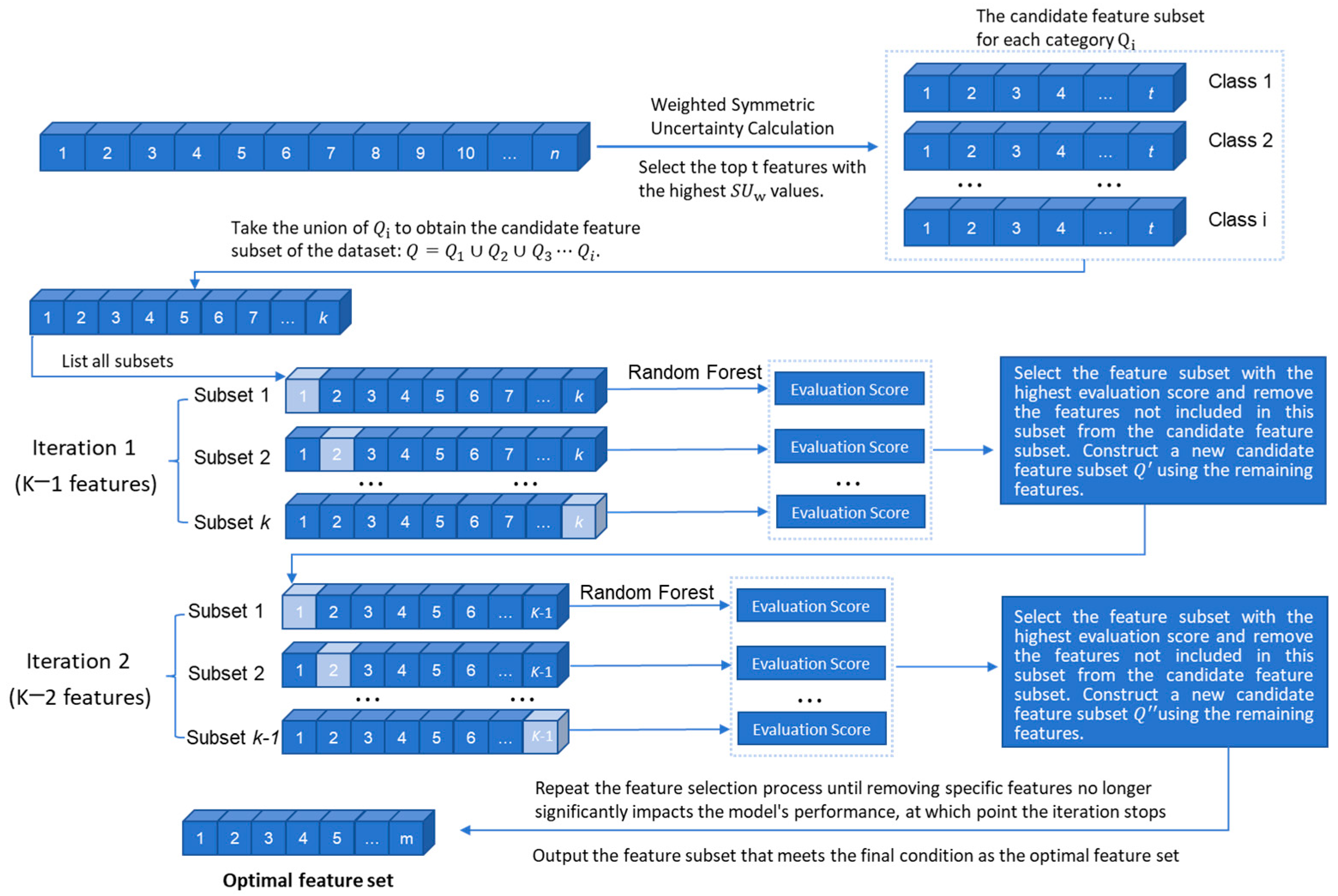
For each row in the matrix, which represents the weighted symmetric uncertainty between different features and class $s_i$, perform a descending sort. For each class $s_i$, select the top t features with the highest weighted symmetric uncertainty values, forming the candidate feature subset $Q_i$ for each class. The union of all these subsets $Q_i$ across all classes forms the overall candidate feature subset $Q=Q_1\cup Q_2\cup \cdots \cup Q_i$.

2.2. Sequential Backward Selection

In feature selection, search algorithms can be divided into exhaustive search, greedy search, and heuristic search. Exhaustive search evaluates all possible feature combinations and, in theory, can find the optimal feature subset in terms of performance. However, its computational complexity grows exponentially with the number of features n (requiring traversal of $2^n-1$ combinations), making it impractical for high-dimensional drilling data. Greedy algorithms include forward search and backward search: forward search starts with an empty set and, at each step, adds the feature that provides the greatest improvement to model performance. While it has low computational cost, it is prone to getting stuck in local optima due to its disregard for feature interactions. Backward search starts from the full feature set and gradually removes features with the least impact on performance, allowing for better consideration of inter-feature relationships. However, since each feature removal requires evaluating its effect on performance, the method involves training on numerous feature combinations, leading to a relatively high computational cost when applied to high-dimensional datasets. Heuristic search methods, such as simulated annealing and genetic algorithms, attempt to find a near-global optimum with lower computational complexity. Simulated annealing avoids local optima by accepting slightly worse solutions, gradually converging over iterations. Genetic algorithms optimize feature subsets through selection, crossover, and mutation operations, but require multiple iterations, leading to higher computational overhead. Considering both computational cost and effectiveness, this paper adopts the sequential backward search algorithm, using random forests to evaluate the quality of the feature set and progressively eliminate redundant features, ensuring a balance between computational efficiency and performance.

The steps of the weighted symmetric uncertainty feature selection process are shown in Figure 1:

• Calculate the weighted symmetric uncertainty between each feature and class, generating the candidate feature subset $Q$;
• For the k features in $Q$, remove one feature to form all possible k−1 subsets. These subsets are input into a random forest model for training, and the subset with the best classification performance is selected;
• Eliminate the features that were not selected and update the candidate feature subset to $Q^{\prime }$;
• Repeat the above steps until removing features no longer significantly impacts the model’s performance, at which point the iteration stops.

The final output feature set not only fully considers the classification needs of minority classes but also effectively incorporates the interactions between features, achieving the goal of precise and efficient feature selection.

3. Sliding-Window-Based SMOTE Oversampling Method

Classical oversampling methods include random oversampling, SMOTE, and its derivative algorithms (such as SMOTE-Tomek, Borderline-SMOTE, and ADASYN) [28]. These methods achieve class balance by either randomly duplicating minority-class samples or generating new samples through interpolation in the feature space [29]. However, different strategies have certain limitations:

• Random duplication of minority-class samples may cause the model to overfit to the characteristics of the minority-class samples. This issue is particularly problematic when the minority class contains noise, as it can further increase the number of anomalous samples;
• Interpolation-based generation of minority-class samples, while leveraging the distribution information of the minority-class samples, may disrupt the temporal relationships in the original data. This can cause the model to learn a distribution that deviates from the true distribution.

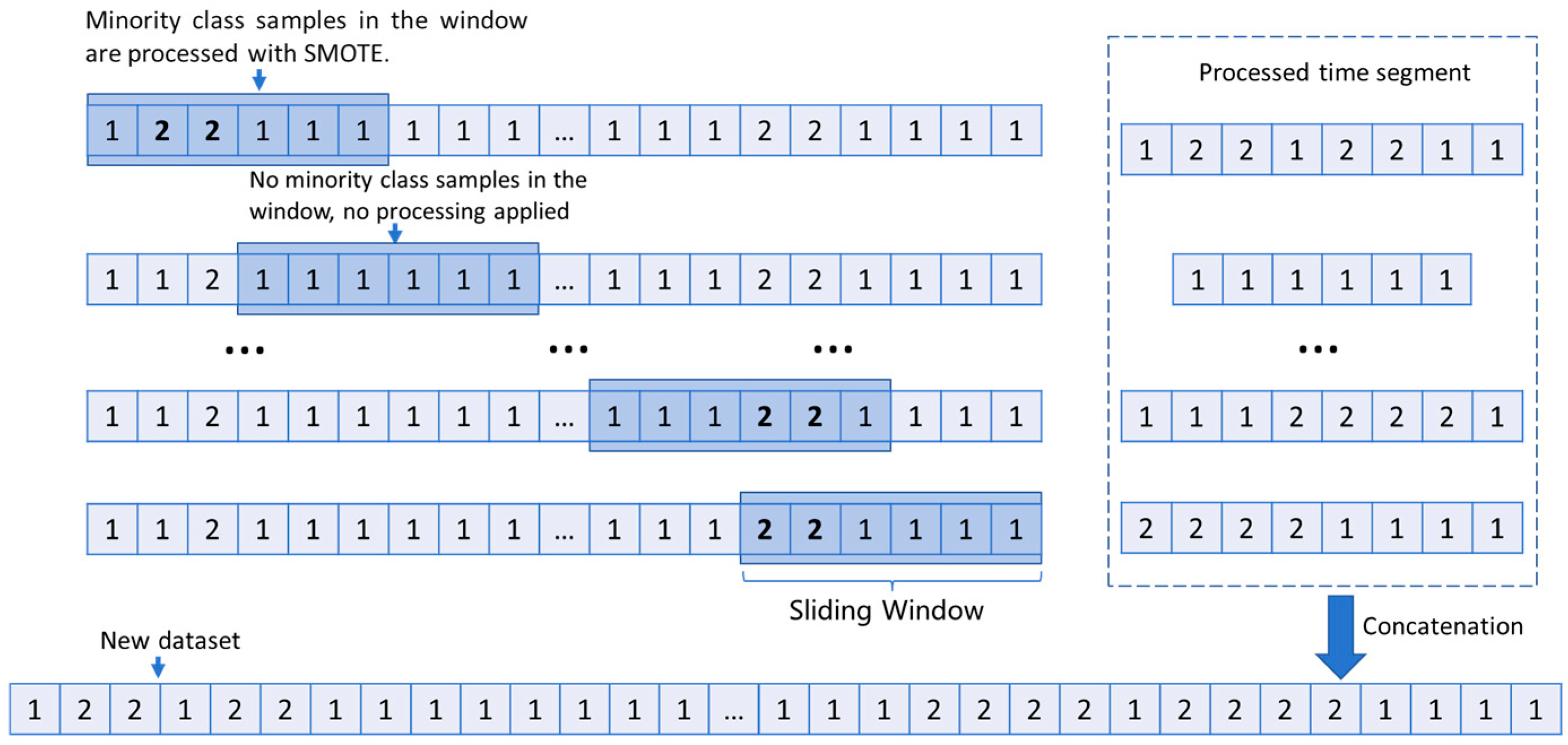
To overcome the aforementioned issues, this paper proposes a sliding-window-based SMOTE oversampling method, which integrates a local temporal preservation mechanism with the SMOTE approach, ensuring the retention of temporal relationships during the synthesis of minority-class samples. First, the drilling time-series data are segmented using a sliding window. Oversampling is then performed within each window, ensuring that the newly generated samples retain the local temporal structure. Meanwhile, the sliding window mechanism enables the gradual expansion of minority-class samples across different segments, overcoming the temporal discontinuities caused by traditional global oversampling. As a result, the generated drilling parameter sequences maintain the continuity of the physical process. By reducing noise interference and enhancing the alignment between the resampled data and the actual distribution, this method significantly improves the quality of data input to the classifier. Consequently, it effectively enhances model classification accuracy and is particularly well suited for applications with strong temporal dependencies, such as drilling state recognition.

3.1. SMOTE Oversampling

SMOTE generates new samples based on the distribution of the minority-class samples by analyzing them, adding these synthetic samples to the original dataset to increase the number of minority-class samples, thus balancing the class distribution and improving the prediction performance of classification algorithms for the minority class [30]. The main steps of the SMOTE method are as follows:

• Neighboring sample set construction: For each minority-class sample, calculate the distance to other minority-class samples using methods like Euclidean distance or Manhattan distance. The k nearest minority-class samples are selected to form the sample’s neighborhood set;
• Random selection of neighboring samples: Based on the class imbalance level q, randomly select q samples from the neighborhood set;
• Generation of new samples: For each original minority-class sample, linear interpolation is performed with the randomly selected q neighboring samples to generate new minority-class samples. The formula for generating new samples is as follows:

  $$x_{new}=x+\alpha \left(x_{nn}-x\right)$$

  (7)

  where $x_{new}$ is the newly generated synthetic sample, x is the original minority-class sample, $x_{nn}$ is the selected neighboring sample, and $\alpha$ is a random number within the range [0, 1] used to control the interpolation ratio. The principle of SMOTE data synthesis is illustrated in Figure 2.

3.2. Sliding Window

Drilling data exhibit strong sequential and temporal dependencies, and traditional oversampling methods may disrupt these temporal dependencies, making it difficult for the model to accurately capture temporal feature information. To address this, by employing a sliding window to segment drilling data, redundant computations during the oversampling process are avoided, effectively reducing the time complexity of data balancing. Additionally, by adjusting the step size, the method provides flexible control over the number of data samples and their overlap, ensuring that SMOTE oversampling expands the minority-class samples while preserving temporal information. Taking binary classification as an example, the SMOTE processing workflow based on the sliding window is illustrated in Figure 3.

• The raw data, window size, and step size are input into the sliding window function, which iterates through the data to segment the continuous drilling time-series into multiple overlapping subsequences. Simultaneously, it extracts drilling parameters, timestamps, and class labels;
• Each subsequence is iterated over, and the proportion of each class label within the current sequence is calculated to distinguish between minority and majority classes:

• If there are minority-class samples within the window (as shown by symbol 2 in Figure 3), linear interpolation is applied to the continuous data within the current window to generate new minority-class samples;
• If there are no minority-class samples within the window, skip this window.

3.

After traversal, concatenate all the segmented subsequences in chronological order to form a new time-series dataset.

Figure 3. Sliding-window-based SMOTE processing flow.

Figure 3. Sliding-window-based SMOTE processing flow.

4. BiLSTM–GRU-Based Classification Model for Drilling Conditions

To balance modeling performance with computational efficiency and reduce the risk of overfitting, this paper explores the application of the BiLSTM–GRU concatenated model in drilling condition classification. The model combines BiLSTM’s ability to capture global context with GRU’s efficient feature compression, demonstrating significant advantages in handling complex, multivariate drilling time-series classification tasks. By adjusting parameters such as the number of network layers and hidden units, the BiLSTM–GRU model can adapt to data characteristics of various scales, enhancing the model’s generalization ability and ensuring robustness and reliability in real-world drilling condition identification. Additionally, its efficient architecture strikes a balance between classification accuracy and computational efficiency, making it suitable for complex drilling scenarios.

4.1. Model Principle

4.1.1. BiLSTM Model

The long short-term memory (LSTM) network is an improved version of the recurrent neural network (RNN), specifically designed to handle time-series data and long-term dependencies. By introducing gating mechanisms, LSTM dynamically controls the retention and forgetting of information, effectively solving the issues of gradient vanishing or explosion that occur in traditional RNNs. This makes LSTM better suited for capturing information from long-term dependencies [31].

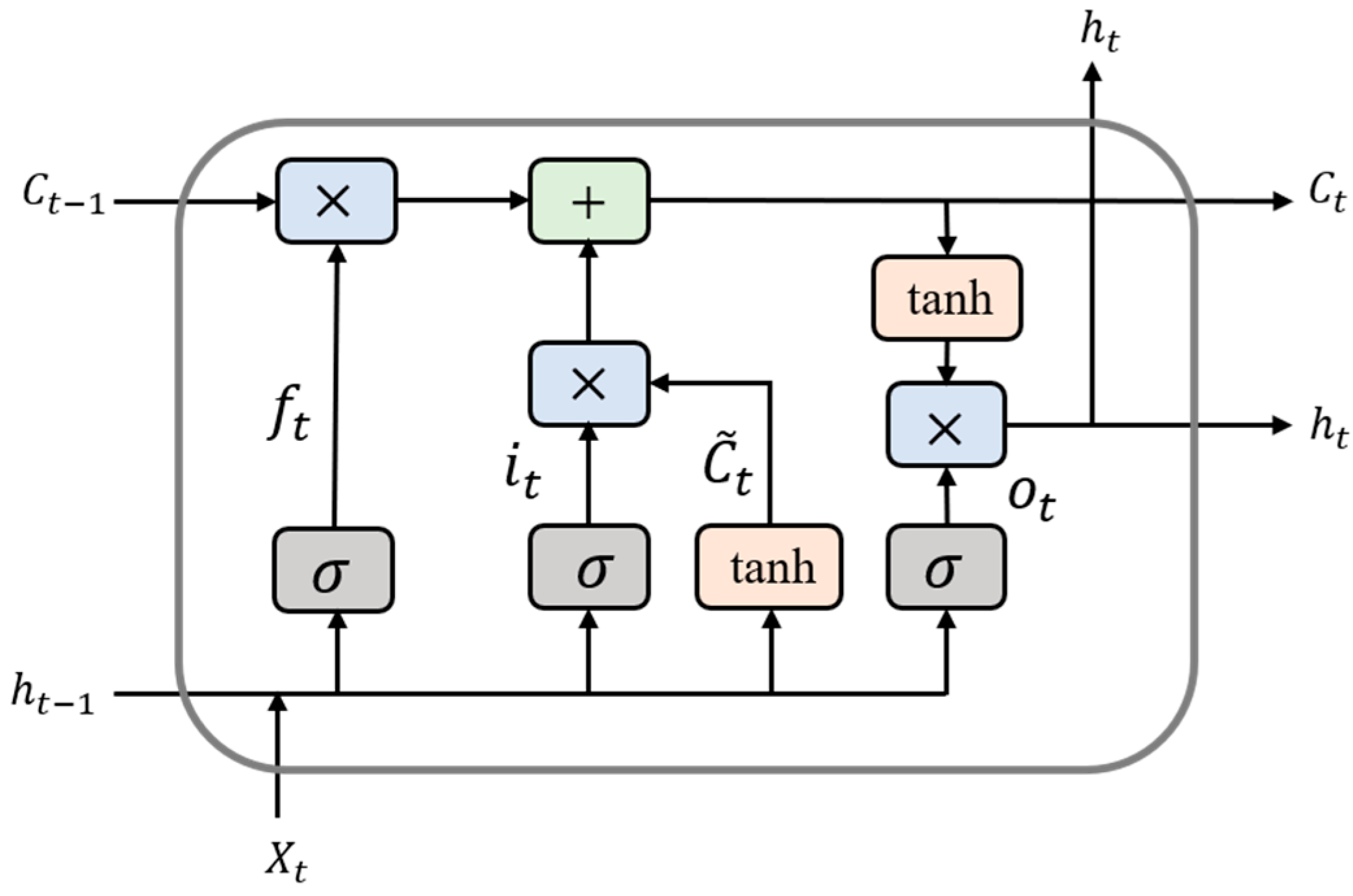
The structure of the LSTM network consists of three gates, as shown in Figure 4:

• Forget gate ($f_t$): Determines the information to discard from the cell state. The input includes the previous hidden state ($h_{t-1}$) and the current input ($X_t$). After passing through a sigmoid function, the output value is between 0 and 1, where 0 means complete discarding and 1 means complete retention;
• Input gate ($i_t$): Controls the update of new information. The sigmoid function selects which values should be updated, while the tanh function generates a candidate state (${\tilde{C}}_t$). The candidate state is then multiplied by the sigmoid result, and the result is added to the previous cell state ($C_{t-1}$) to update the current cell state ($C_t$);
• Output gate ($o_t$): Determines the output of the hidden state. The current cell state ($C_t$) is processed through the tanh function, and the result is multiplied by the output of the sigmoid function to generate the current hidden state ($h_t$), thereby considering both the current input and the long-term memory.

The computational expressions for the LSTM network are as follows:

$$f_t=\sigma \left(W_f{h}_{t-1}+U_f{X}_t+b_f\right)$$

(8)

$$i_t=\sigma \left(W_i{h}_{t-1}+U_i{X}_t+b_i\right)$$

(9)

$$o_t=\sigma \left(W_o{h}_{t-1}+U_o{X}_t+b_o\right)$$

(10)

$${\tilde{C}}_t=tan h\left(W_c{h}_{t-1}+U_c{X}_t+b_c\right)$$

(11)

$$C_t=f_t\times c_{t-1}+i_t\times {\tilde{C}}_t$$

(12)

$$h_t=o_t\times tan h\left(C_t\right)$$

(13)

where $\sigma$ is the sigmoid activation function. $W_f$,$W_i$,$W_o$,$W_c$ are the weight matrices for the gate units and state units. These matrices are used to linearly transform the previous hidden state $h_{t-1}$. $U_f$,$U_i$,$U_o$,$U_c$ are the weight matrices for the gate units and state units. These matrices are used to linearly transform the current input $X_t$. $b_f$, $b_i$, $b_o$,$b_c$ are the bias terms for the gate units and state units.

The structure of the BiLSTM network is shown in Figure 5, consisting of a forward LSTM and a backward LSTM. The forward LSTM processes the input data in normal sequential order. For example, for the drilling sequence data $X=\left(X_0,X_1,X_2, \dots ,X_T\right)$, the forward LSTM starts from $X_0$ and calculates the forward hidden state $\overrightarrow{h_t}$ at time step t, then sequentially processes $X_1,X_2,\dots ,X_T$. In contrast, the backward LSTM processes the input data in reverse order, starting from $X_T$ and calculating the backward hidden state $\overleftarrow{h_t}$ at time step t, then sequentially processes $X_{T-1},X_{T-2},\dots ,X_0$. The output of the BiLSTM is obtained by concatenating the forward and backward hidden states. Specifically, for each time step t, the output is $Y_t=\left[\overrightarrow{h_t},\overleftarrow{h_t}\right]$. The BiLSTM model comprehensively considers both the past trends (forward) and future trends (backward) of sequence data, providing more comprehensive feature information for condition classification and prediction.

4.1.2. GRU Model

GRU is a variant of the LSTM structure with a simplified design. It combines the input gate and forget gate of LSTM into a single update gate and merges the cell state with the hidden state. With the same number of hidden units, the GRU model has lower computational cost and faster training speed compared to the LSTM model, especially when processing large volumes of drilling data. This makes GRU more efficient for training on extensive datasets [32].

The GRU network structure consists of two gates, as shown in Figure 6:

Update gate ($z_t$): This gate determines how much of the previous memory should be retained and how much new information should be added at the current time step. Its input is the previous hidden state ($h_{t-1}$) and the current input ($X_t$), which, after passing through the sigmoid function, produces an output value ($z_t$) between 0 and 1. When $z_t$ is closer to 1, it indicates that more of the previous state information is retained; when it is closer to 0, it suggests that more reliance is placed on the current input to update the state.

Reset gate ($r_t$): This gate controls how much of the previous memory should be retained. Its input is the previous hidden state ($h_{t-1}$) and the current input ($X_t$). The output ($r_t$) is also a value between 0 and 1, and it is used to control the impact of the previous hidden state ($h_{t-1}$) on the current computation. When the reset gate output is 0, the previous hidden state is ignored; when it is 1, the previous hidden state is fully considered.

The candidate hidden state ${\tilde{h}}_t$ is obtained by concatenating and linearly transforming the scaled previous hidden state $h_{t-1}$ (adjusted by the reset gate) and the current input $X_t$. The current hidden state $h_t$ is then computed by using the update gate’s output to control the relative contributions of the previous hidden state $h_{t-1}$ and the candidate hidden state ${\tilde{h}}_t$. The update gate dynamically balances historical information and new data, allowing the hidden state to effectively capture changes and patterns in sequence data. This mechanism helps avoid the issues of vanishing and exploding gradients when processing long sequences, thus enabling better learning of long-term dependencies.

The computational expressions for the GRU are as follows:

$$z_t=\sigma \left(W_z{X}_t+U_z{h}_{t-1}+b_z\right)$$

(14)

$$r_t=\sigma \left(W_r{X}_t+U_r{h}_{t-1}+b_r\right)$$

(15)

$${\tilde{h}}_t=tan h\left(W_h{X}_t+U_h\left(r_t\times h_{t-1}\right)+b_h\right)$$

(16)

$$h_t=\left(1-z_t\right)\times h_{t-1}+z_t\times {\tilde{h}}_t$$

(17)

where $\sigma$ is sigmoid activation function, $W_z$, $W_r$,$W_h$,$U_z$,$U_r$,$U_h$ are the weight matrices, and $b_z,b_r$,$b_h$ are the bias terms.

4.2. BiLSTM–GRU Model

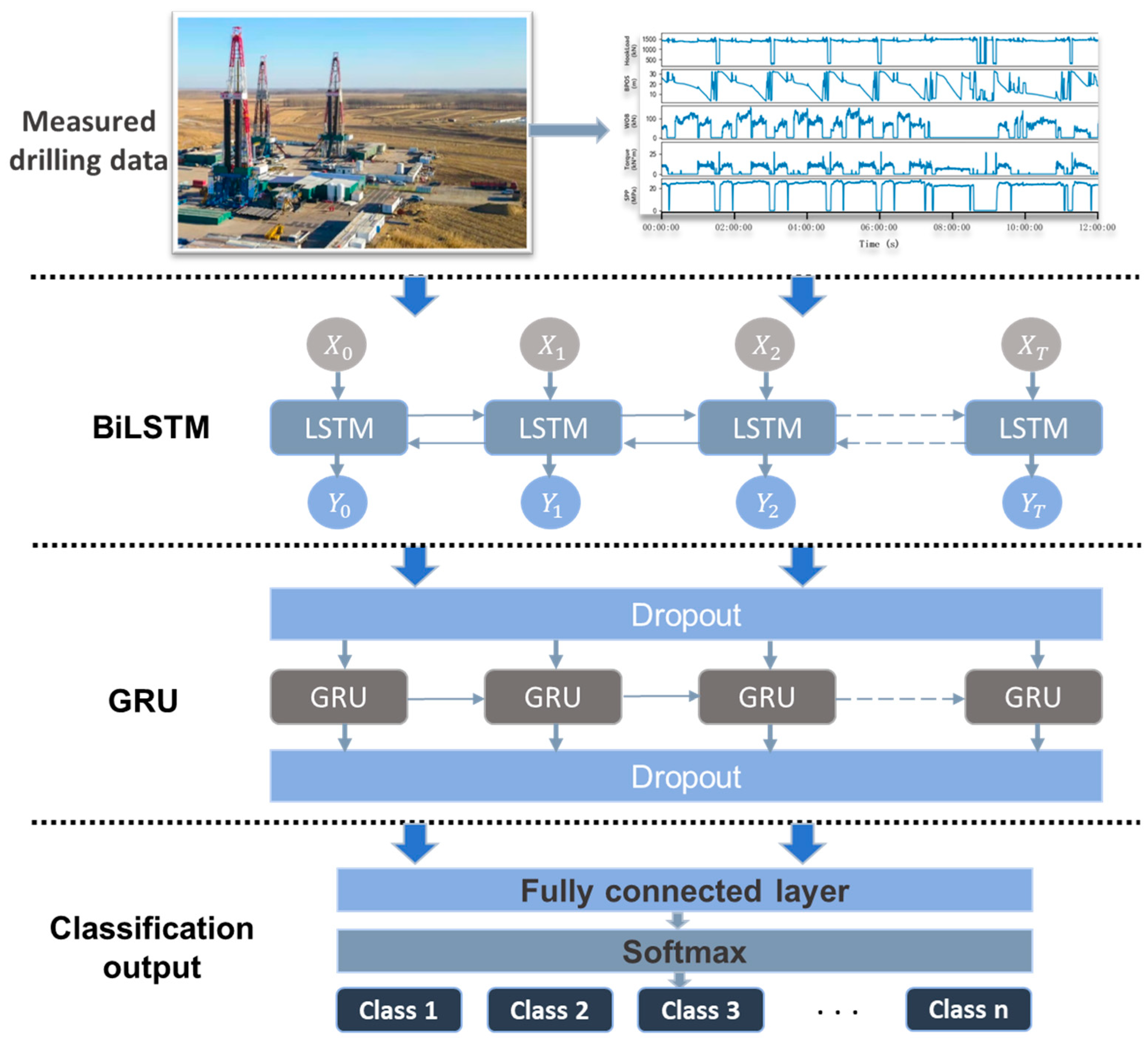
The structure of the BiLSTM–GRU concatenated model is shown in Figure 7. The model’s input is a three-dimensional tensor with the shape $\left(m,t,n\right)$, where m is the number of samples in the drilling sequence data, t is the time steps, and n is the number of features contained in the dataset. The model’s output is the probability distribution for each class, which is used to predict the operational condition corresponding to the input data. After the data are input, they first pass through the BiLSTM layer, enabling the model to capture both forward and backward information from the input sequence. This allows the model to learn bidirectional dependencies and complex temporal features in the time-series data, providing rich representations for subsequent layers. Following the BiLSTM layer, the output sequence is fed into a dropout layer. During training, the dropout layer randomly sets a portion of the neuron outputs to zero, effectively “dropping out” a certain number of neurons. This prevents the model from relying excessively on specific neurons, thus enhancing its generalization ability on new data and mitigating overfitting. The output of the dropout layer is then input into the GRU model, which performs a higher-level time-series pattern extraction based on the BiLSTM model, emphasizing the key temporal information and improving the quality of temporal feature representation. The sequence output by the GRU is further passed through another dropout layer, further enhancing the model’s generalization capability. Following the dropout layer, a fully connected layer is applied, where an activation function introduces nonlinearity, allowing the model to learn the complex nonlinear relationships between the drilling data features. The output of the fully connected layer is processed by the softmax activation function, converting the output into a probability distribution across the different classes. The class with the highest probability is selected as the predicted result, thus achieving the multi-class classification task for drilling conditions.

5. Experiment and Analysis of Drilling Condition Identification

5.1. Model Evaluation Indicators

In the study of classification problems, the confusion matrix serves as an effective tool for representing prediction results, providing a clear presentation of the various situations that may arise during the model’s prediction process [33]. For binary classification, the confusion matrix compares the model’s predicted values with the actual labels of the data to assess the model’s performance.

Specifically, True Positive (TP) refers to the number of positive samples that the model correctly classifies as positive. True Negative (TN) represents the number of negative samples that the model correctly classifies as negative. False Positive (FP) refers to the number of negative samples that the model incorrectly predicts as positive. False Negative (FN) indicates the number of positive samples that the model incorrectly predicts as negative. These metrics are crucial for evaluating the performance of classification models, including accuracy, precision, recall, and F1 score. Accuracy represents the proportion of correctly predicted samples among the total number of samples. Precision measures the proportion of actual positive samples among those predicted as positive, reflecting the model’s prediction accuracy. Recall refers to the proportion of positive samples that the model correctly identifies, indicating the model’s ability to detect positive cases. The F1 score is the harmonic mean of precision and recall, combining the model’s prediction accuracy and recall ability, providing a more valuable reference for performance evaluation and improvement. The formulas for calculating these evaluation metrics are as follows:

$$Accuracy={\displaystyle \frac{TP+TN}{TP+TN+FP+FN}}$$

(18)

$$recision={\displaystyle \frac{TP}{TP+FP}}$$

(19)

$$Recall={\displaystyle \frac{TP}{TP+FN}}$$

(20)

$$F1={\displaystyle \frac{2\times Precision\times Recall}{Precision+Recall}}$$

(21)

5.2. Data Processing and Model Design

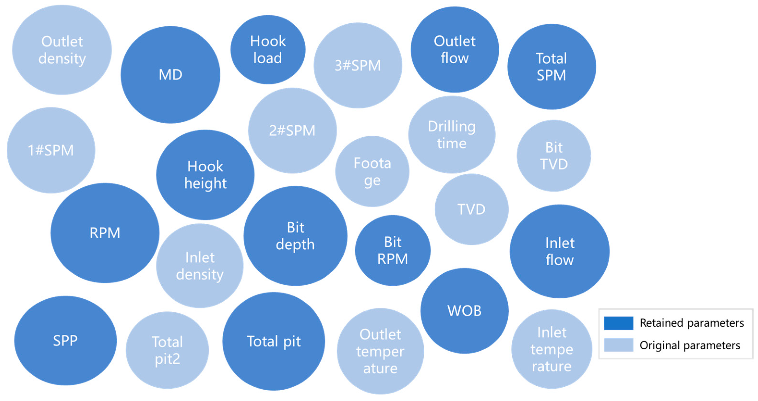
The dataset used in this study originates from the actual logging data of 14 adjacent wells in Block H of an oilfield, all from the same drilling cycle, totaling 194,035 data points. The model is built using Python (3.11) and the TensorFlow (2.17) deep learning framework, with sklearn (1.5.2) for data evaluation and processing. Additionally, matplotlib (3.9.2) and seaborn (0.13.2) are utilized for visualizing the training process. To address anomalies or missing data caused by equipment failures, communication issues, and other factors, the boxplot analysis method was employed for data cleaning. First, missing and blank values were removed, and outliers were handled. To prevent differences in the dimensions of drilling parameters from affecting feature importance and correlation, the Z-score normalization method was applied to the data prior to feature engineering. The original dataset contained 25 parameters, including wellbore depth, vertical depth, bit position, and drilling pressure. After feature engineering using a weighted symmetric uncertainty-based feature selection method, 12 drilling parameters were selected. The original parameters and the parameters retained after feature selection are shown in Figure 8.

In conjunction with the drilling work logs, the data were labeled with nine drilling conditions, with the proportion of each condition in the original dataset and the corresponding label assignments shown in

Table 1. Proportions of each condition and label settings before and after class imbalance handling.

Condition	Original Data		Processed Data After Oversampling		Label
	Sample Size	Percentage	Sample Size	Percentage
Rotary drilling	40,159	20.70%	40,159	11.11%	0
Sliding drilling	18,977	9.78%	40,159	11.11%	1
Trip out	21,423	11.04%	40,159	11.11%	2
Trip in	25,378	13.08%	40,159	11.11%	3
Making a connection	34,851	17.96%	40,159	11.11%	4
Stationary (drilling)	23,740	12.23%	40,159	11.11%	5
Drilling break cycle	14,571	7.51%	40,159	11.11%	6
Drilling break cycle + rotation	11,947	6.16%	40,159	11.11%	7
Bottom hole spinning	2989	1.54%	40,159	11.11%	8

. The proportion differences between the conditions in the original data were significant, and the imbalance rate between the majority and minority classes in this dataset reached 13.43.

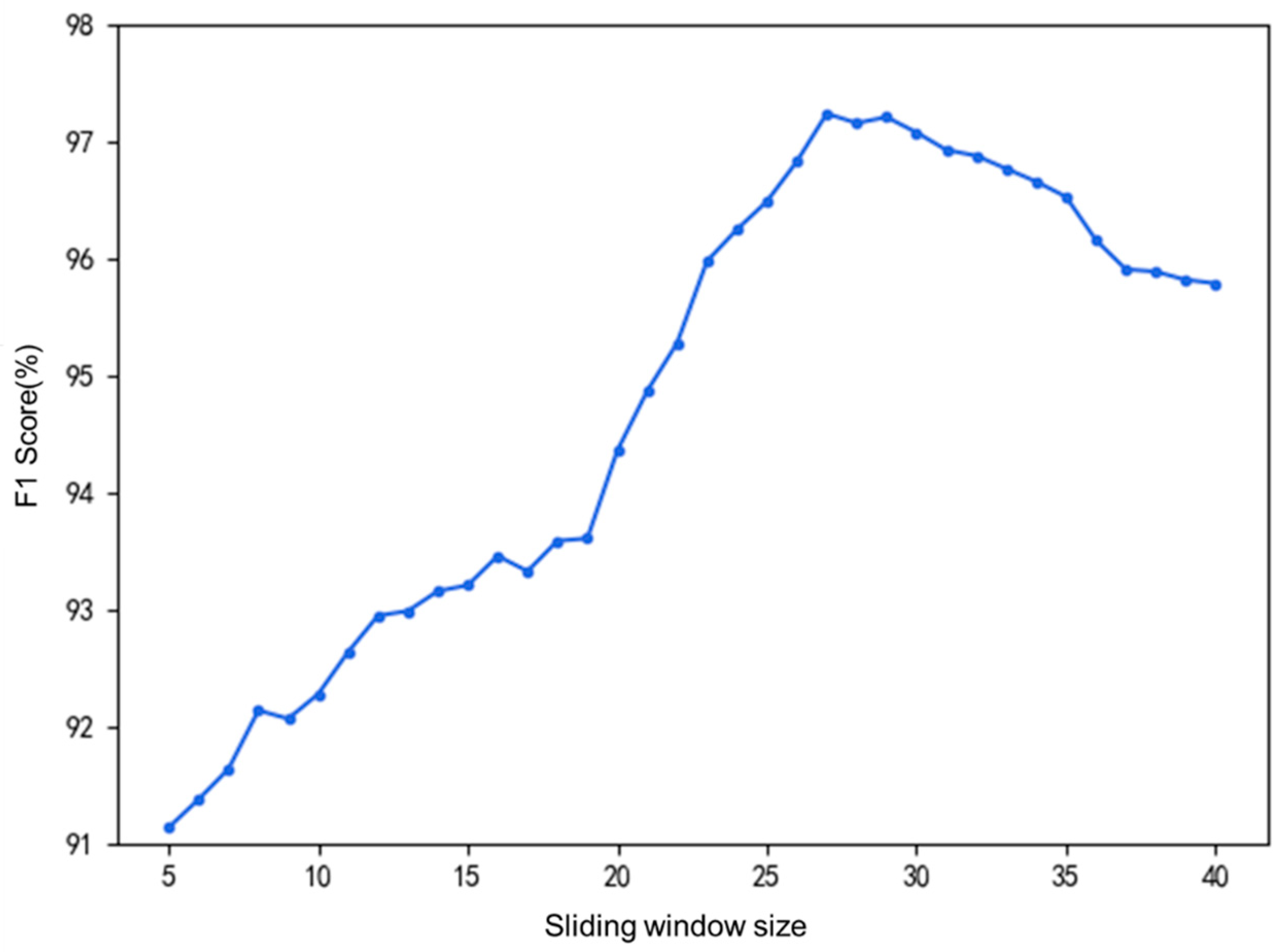
When using the sliding-window-based SMOTE oversampling method, the choice of window size and time step significantly affects the results. The window size determines the local segment range of the data during each resampling, while the time step determines the distance the sliding window moves each time. To preserve the dependencies between adjacent time points in the drilling time-series data, the time step is set to half of the window size. To select an appropriate sliding window size, the window size is increased from 5 to 40, and the synthetic dataset is input into the classifier for training. The relationship between the model’s classification F1 score and the sliding window size is shown in Figure 9. The final window size is determined to be 24, and after applying the sliding-window-based SMOTE method for oversampling, the class distribution of the different drilling conditions becomes balanced.

To optimize the model performance, hyperparameter configurations were adjusted based on key indicators such as precision, recall, loss value, and training time on the test set. The detailed hyperparameter settings are shown in

Table 2. Hyperparameter settings for the BiLSTM–GRU model.

Model	Network Architecture	Parameter Setting
BiLSTM	Number of neurons	128
	Dropout	0.5
	Return sequences	True
GRU	Number of neurons	128
	Dropout	0.5
	Return sequences	True
Full connectivity layer	Number of neurons	(12,864)
	Activation function	ReLU
Other	Learning rate	0.001
	Batch size	64

. For the BiLSTM model, the number of hidden units is set to 128. To enable the network to better handle long-term dependencies in sequential data, the BiLSTM model outputs the full sequence as input for subsequent recurrent layers. The data undergo a dropout layer with a dropout rate of 0.5 both when inputting to the GRU model and when outputting, which randomly discards half of the neurons to prevent over-reliance on specific neurons, thus improving the model’s generalization ability. The number of hidden units in the GRU model is also set to 128. To reduce data dimensionality and highlight the most important feature information, two fully connected layers are used with 128 and 64 neurons, respectively. The activation function for both layers is ReLU (Rectified Linear Unit). Finally, the data are input into a softmax layer for classification, with the output having nine categories corresponding to nine different drilling condition labels. The model is compiled using the Adam (Adaptive Moment Estimation) optimizer and the F1 score as the evaluation metric, with the learning rate set to 0.001. Since drilling condition classification is a multi-class classification task, sparse categorical cross-entropy is chosen as the loss function, and the predicted values input into the loss function are the probabilities processed by the softmax activation function. The dataset is divided into a training set and a test set in a 7:3 ratio, with the number of samples input into the model for each iteration set to 64.

5.3. Analysis of the Effect of Feature Selection on Model Performance Improvement

To validate the effect of feature selection based on weighted symmetric uncertainty on model performance, a comparison is made with the predictive results of classifiers under various feature selection methods, including no feature selection, variance threshold filtering, the chi-squared test, and extreme gradient boosting feature selection. Among them, variance threshold filtering and the chi-squared test are filtering methods in feature selection. Variance threshold filtering calculates the variance of each feature and determines whether to remove the feature from the dataset based on whether its variance is below the set threshold. The chi-squared test measures the correlation between categorical features and the target variable through statistical tests, calculating the chi-squared statistic and p-value using a contingency table to determine whether a significant relationship exists between the feature and the target variable. Extreme gradient boosting, belonging to the embedding methods of the three main feature selection categories, computes the contribution of each feature in building the tree model during training to assess feature importance. The feature selection process is completed based on the ranking of feature importance. Accuracy, precision, recall, and F1 score are selected as performance evaluation metrics for the models. A comparison of the model performance improvements under different feature selection algorithms is shown in Figure 10.

As shown in the figure, after applying the feature selection based on weighted symmetric uncertainty to the dataset and training the model, the model’s accuracy, precision, recall, and F1 score improved by 1.56%, 3%, 3%, and 3%, respectively, compared to the dataset without feature selection. The feature selection method based on weighted symmetric uncertainty outperformed the variance threshold filtering and chi-squared test filtering methods, as well as the embedding-based extreme gradient boosting feature selection method. Specifically, the model accuracy improved by 0.29%, 0.47%, and 0.2%, precision improved by 2%, 2%, and 2%, recall improved by 3%, 4%, and 3%, and the F1 score improved by 3%, 3%, and 3%, respectively.

5.4. Analysis of the Effect of Oversampling on Model Performance Improvement

To validate the effect of the sliding-window-based SMOTE oversampling method on the performance improvement of model recognition for different drilling conditions, the drilling data processed using the sliding-window-based SMOTE oversampling method will be compared with the original data and datasets resampled using other synthetic oversampling methods such as random oversampling, SMOTE, SMOTE-Tomek [34], Borderline-SMOTE [35], and ADASYN [36]. These datasets will be input into the BiLSTM–GRU classification model for training. The recognition precision, recall, and F1 score for each condition under different oversampling methods are shown in

Table 3. Comparison table of drilling condition recognition precision under different oversampling methods.

Oversampling Method	Precision
	Rotary Drilling	Sliding Drilling	Trip Out	Trip in	Making a Connection	Stationary (Drilling)	Drilling Break Cycle	Drilling Break Cycle + Rotation	Bottom Hole Spinning
Original data	95%	85%	87%	87%	94%	88%	87%	89%	85%
Random oversampling	95%	91%	94%	92%	93%	92%	92%	96%	99%
SMOTE	95%	93%	94%	93%	95%	92%	92%	96%	99%
SMOTE-Tomek	96%	92%	91%	92%	92%	89%	92%	96%	98%
Borderline-SMOTE	94%	91%	94%	95%	94%	92%	94%	97%	99%
ADASYN	97%	91%	96%	96%	89%	89%	95%	98%	99%
Sliding-window-based SMOTE	99%	100%	98%	98%	98%	97%	99%	98%	100%

,

Table 4. Comparison table of drilling condition recognition recall under different oversampling methods.

Oversampling Method	Recall
	Rotary Drilling	Sliding Drilling	Trip Out	Trip in	Making a Connection	Stationary (Drilling)	Drilling Break Cycle	Drilling Break Cycle + Rotation	Bottom Hole Spinning
Original data	96%	92%	91%	90%	92%	90%	78%	87%	78%
Random oversampling	95%	95%	91%	94%	91%	92%	90%	95%	98%
SMOTE	96%	92%	94%	91%	92%	95%	93%	96%	98%
SMOTE-Tomek	96%	93%	91%	94%	89%	92%	91%	95%	98%
Borderline-SMOTE	97%	95%	92%	97%	92%	94%	91%	96%	98%
ADASYN	98%	96%	93%	98%	91%	89%	89%	96%	98%
Sliding-window-based SMOTE	98%	99%	98%	99%	98%	98%	99%	98%	100%

and

Table 5. Comparison table of drilling condition recognition F1 score under different oversampling methods.

Oversampling Method	F1 Score
	Rotary Drilling	Sliding Drilling	Trip Out	Trip in	Making a Connection	Stationary (Drilling)	Drilling Break Cycle	Drilling Break Cycle + Rotation	Bottom Hole Spinning
Original data	96%	88%	89%	88%	93%	89%	82%	88%	81%
Random oversampling	96%	93%	91%	94%	89%	92%	91%	95%	98%
SMOTE	96%	92%	94%	92%	93%	94%	92%	96%	98%
SMOTE-Tomek	96%	92%	91%	93%	91%	91%	92%	96%	98%
Borderline-SMOTE	96%	93%	93%	96%	93%	93%	93%	96%	98%
ADASYN	97%	93%	94%	97%	90%	89%	92%	97%	99%
Sliding-window-based SMOTE	98%	100%	98%	98%	98%	98%	99%	98%	100%

.

From Table 3, Table 4 and Table 5, it can be observed that after training the classification model on the original dataset, there are significant differences in precision, recall, and F1 scores across different classes. For example, in terms of the F1 score, the proportion of rotary drilling and making-a-connection samples in the original dataset is 20.70% and 17.96%, respectively, making them majority classes. Their classification F1 scores reach 96% and 93%, respectively. In contrast, bottom hole spinning accounts for only 1.54% of the original data, making it a minority class, and its classification F1 score is only 81%. These results indicate that when classifying the original drilling data, there is a substantial disparity in classification performance across different categories. Minority-class samples are frequently misclassified, while the overall classification performance of the model appears strong due to the high accuracy in majority classes. This imbalance prevents the model from truly reflecting its performance across all categories, making it unreliable for accurately estimating and making decisions about different drilling conditions. Consequently, the overall classification performance of the model lacks practical value. Using the sliding-window-based SMOTE oversampling method, the precision, recall, and F1 scores for all operating conditions were improved to the 98–100% range. For the less-frequent conditions in the original dataset, such as drilling break cycle, drilling break cycle + rotation, and bottom hole spinning, the classification performance showed no significant difference compared to the majority classes like rotary drilling and sliding drilling. This result indicates that after processing the dataset with the sliding-window-based SMOTE oversampling method, the classifier training did not suffer from performance disparities caused by class imbalance. The model’s classification results are reliable, demonstrating the classifier’s practical applicability in handling imbalanced drilling condition datasets.

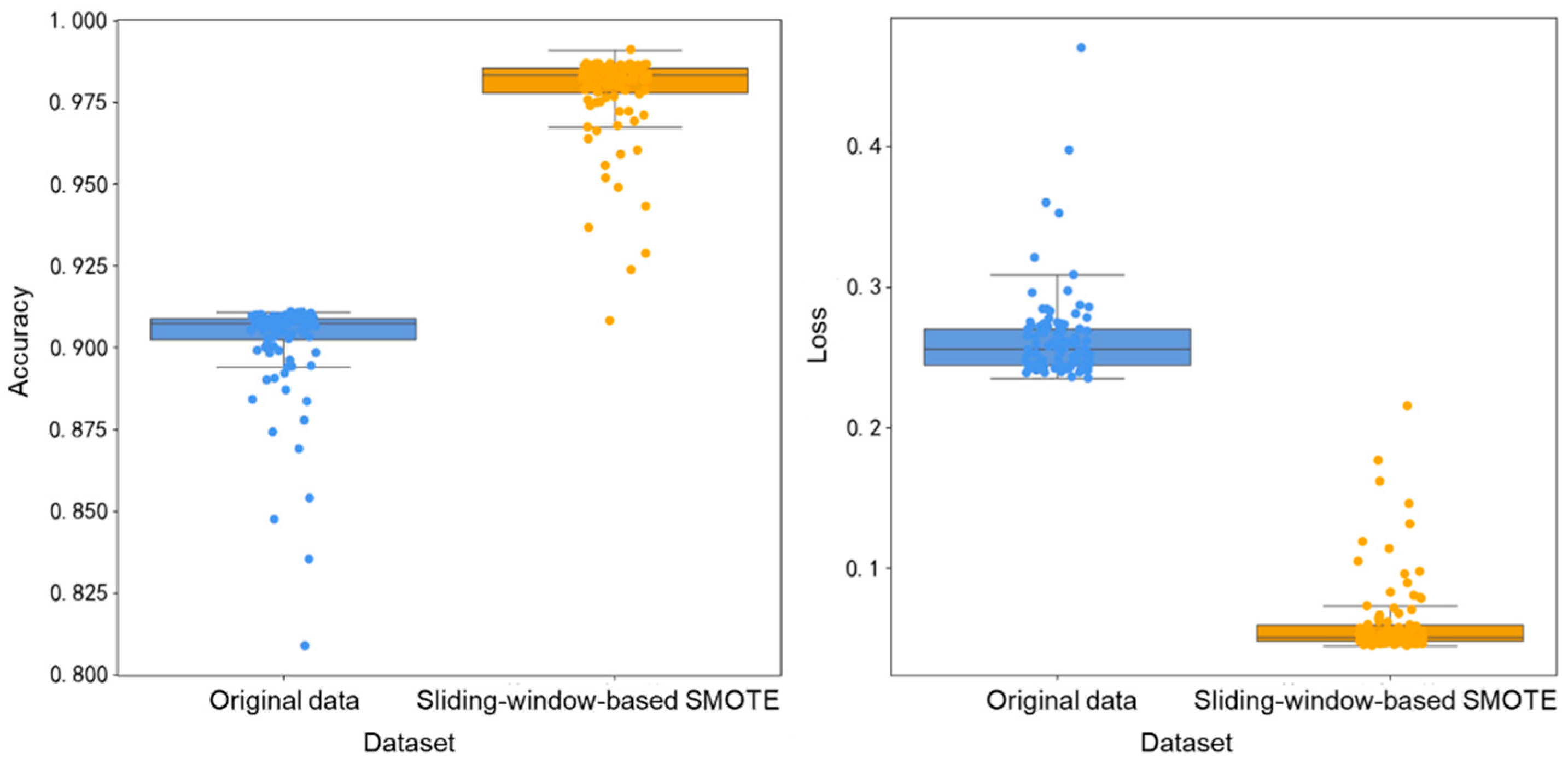
To validate the overall accuracy and fitting degree of the model trained using the sliding-window-based SMOTE oversampling method, both the original dataset and the dataset after sliding-window-based SMOTE oversampling were input into the model for training. The distribution of accuracy and loss values on the test set during 100 iterations of training is shown in Figure 11. As can be seen from the figure, compared to the original data without class balancing treatment, when the model was trained with the resampled dataset, the training accuracy increased from 91.72% to 98.70%, and the training loss decreased from 0.2856 to 0.0450. Moreover, the distribution of accuracy and loss values became more concentrated. In conclusion, after performing data augmentation on the drilling dataset, the model’s fitting to the data improved, and both the recognition performance for various drilling conditions and the overall classification performance of the model were enhanced.

5.5. Analysis of the Classification Performance of the BiLSTM–GRU Model

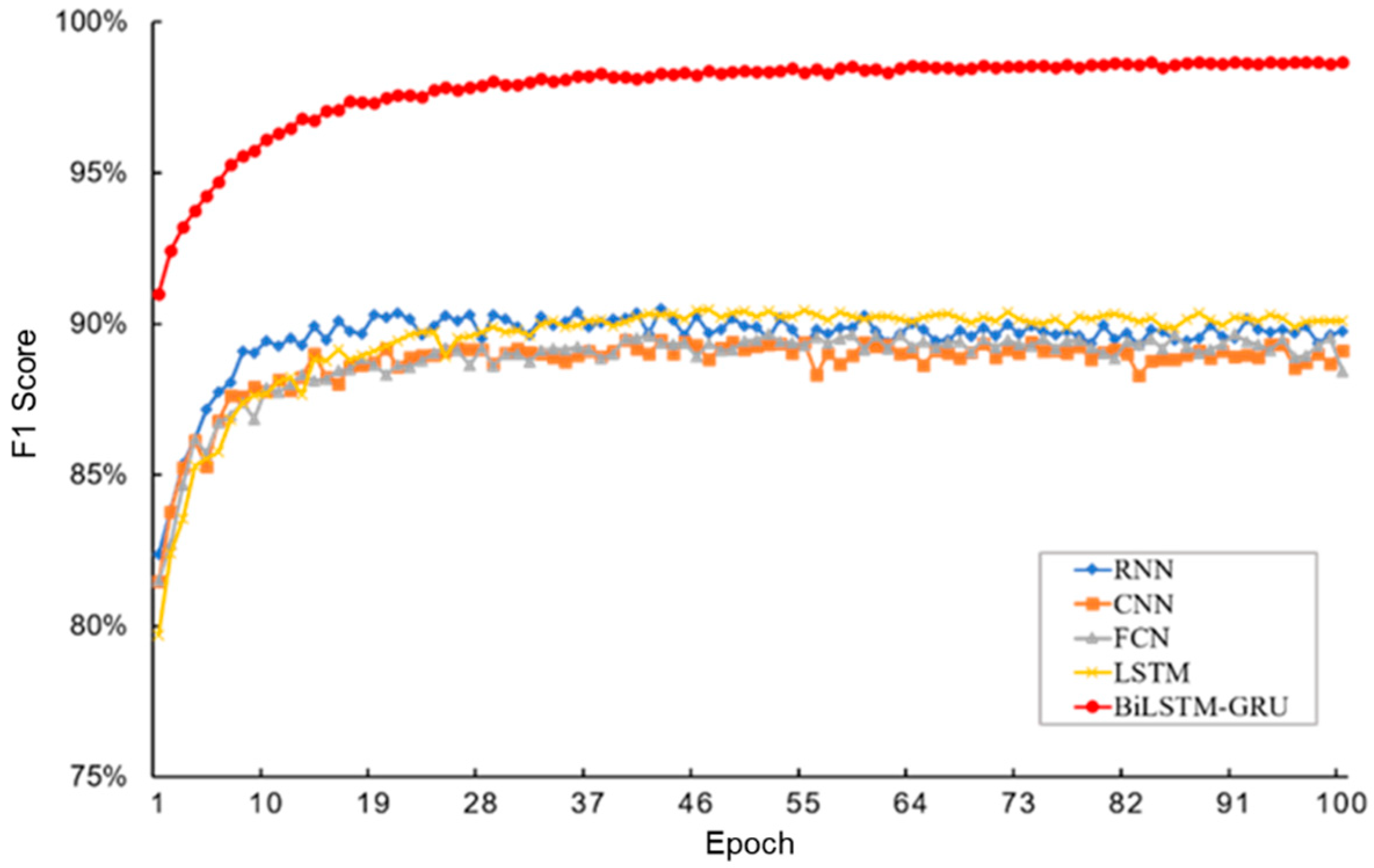
To validate the performance improvement of the BiLSTM–GRU model in drilling condition classification prediction, four commonly used classification models were selected for comparison. The F1 score variation curve of the test set during training for different models is shown in Figure 12. Compared to the RNN (recurrent neural network), CNN (convolutional neural network), FCN (fully convolutional network), and LSTM models, the F1 scores of the BiLSTM–GRU model in this paper improved by 8.95%, 9.58%, 10.25%, and 8.59%, respectively. 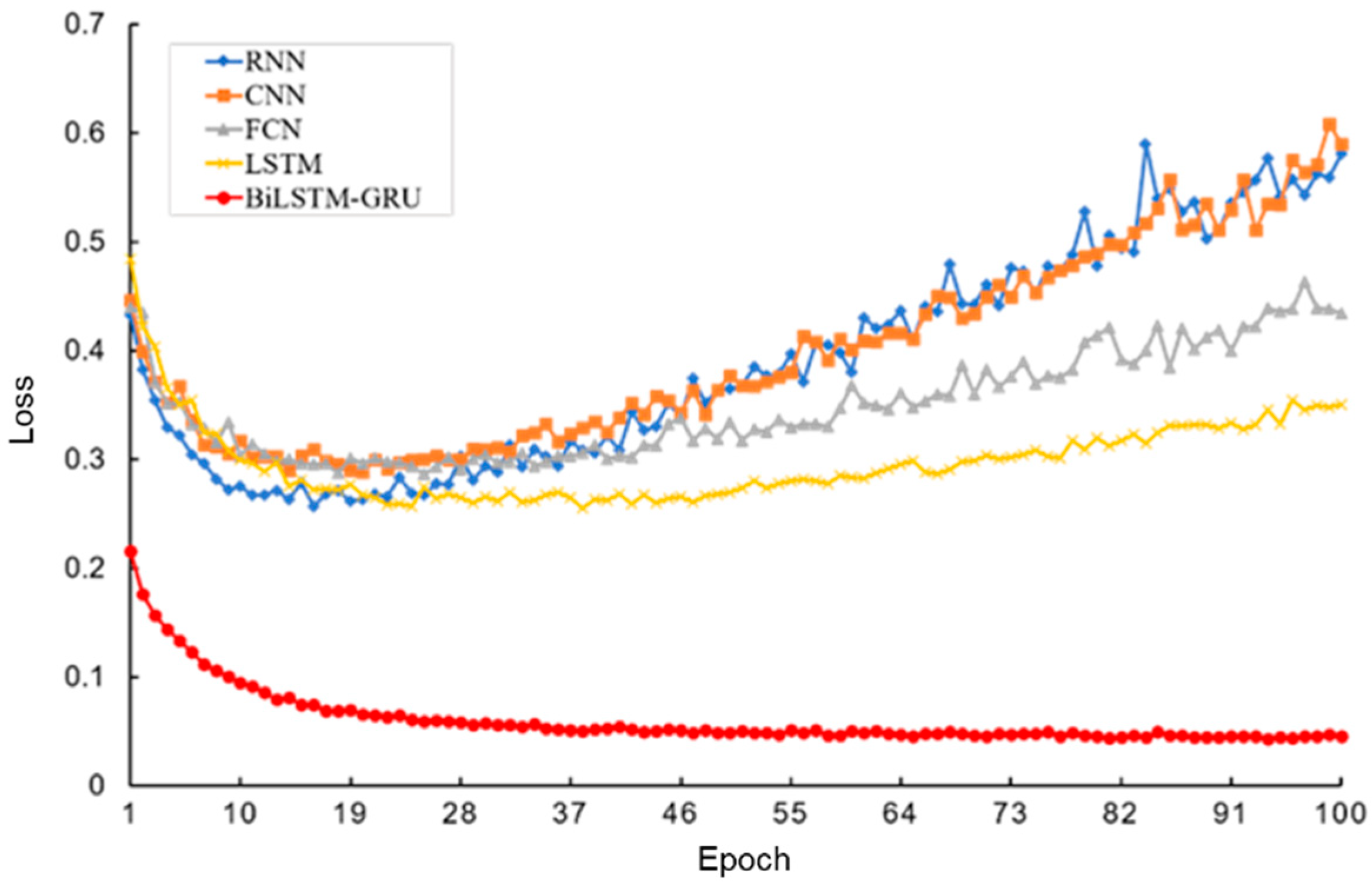Moreover, the F1 score of the BiLSTM–GRU model did not stagnate or decline in the later stages of training, indicating that the learning process of the model is stable and can continuously extract useful information from the data to improve its performance. The loss value variation curve of the test set during training for different models is shown in Figure 13. Compared to the RNN, CNN, FCN, and LSTM models, the loss value of the BiLSTM–GRU model in this paper decreased by 0.32, 0.3315, 0.2893, and 0.2246, respectively. Other models showed varying degrees of loss value increase in the later stages of training, indicating that they overlearned noise, outliers, and other special patterns in the training data, leading to overfitting and loss of the ability to grasp general patterns. In contrast, the loss value of the BiLSTM–GRU model steadily decreased without any increasing trend, demonstrating its good generalization ability. The variation curves of F1 score and loss value during the training process suggest that the BiLSTM–GRU model proposed in this paper has a good fit to the drilling data patterns, with reasonable model parameter settings and strong generalizability.

Using the BiLSTM-FCN model to predict the categories of drilling data generated within 48 h, the confusion matrix of the classification results is shown in Figure 14. In the figure, the number of samples on the main diagonal is significantly higher than that of the off-diagonal elements, indicating that the model, trained with the dataset processed through data augmentation, demonstrates high classification accuracy and stability. Additionally, the classification prediction performance across different categories is relatively balanced, with no shift in classification results towards the majority class.

The above experimental results demonstrate that the drilling condition recognition method proposed in this paper, which is tailored for imbalanced datasets, effectively addresses the impact of class imbalance on model classification results. The BiLSTM–GRU composite model constructed in this paper enhances the accuracy of condition classification prediction and exhibits good generalization ability.

6. Conclusions

To address the class imbalance issue in drilling condition data, a feature selection method based on weighted symmetric uncertainty is proposed. This method enhances the weight of minority class features by applying weighting, optimizing the class contrast. Compared to methods such as variance threshold filtering, the chi-squared test, and extreme gradient boosting, this approach effectively improves the model’s performance: accuracy increased by 0.29%, 0.47%, and 0.2%, precision increased by 2%, recall increased by 3%, and F1 score improved by 3%.

To preserve the temporal characteristics of drilling data, a sliding-window-based SMOTE oversampling method is proposed. By segmenting and concatenating subsequences, this method balances the number of conditions for each class while maintaining the time-series features of the data. After applying oversampling, the BiLSTM–GRU model trained on the data achieved condition recognition accuracy, recall, and F1 scores in the range of 98–100%, with balanced accuracy across all categories.

The proposed weighted symmetric uncertainty feature selection and sliding-window-based SMOTE oversampling collaborative optimization method also holds significant application value in typical small-sample, high-risk scenarios such as drilling equipment fault diagnosis and stuck pipe accident prediction. By optimizing class contrast and preserving temporal features, this approach reduces the probability of missed alarms, enhances fault identification performance, and provides strong support for the safe and efficient operation of drilling activities.

The model’s transferability needs improvement, as it cannot be fully adapted to drilling condition analysis across different oilfield blocks. Given the multidimensional nature of drilling condition data, it is recommended to extend the existing model by integrating a multi-task learning framework, combining tasks such as condition recognition, drilling efficiency prediction, and risk assessment, to enhance the model’s overall performance in practical applications.

References

- Liu, W.; Tang, C.; Fu, J.; Song, X.; Xu, B.; Ji, Y. Research progress of early identification and safety control of well kick and lost circulation complexities. China Pet. Mach. 2023, 51, 9–16. [Google Scholar] [CrossRef]
- Wang, X.; Zhang, F.; Li, Z.; Wang, Y.; Fang, H. Real-time intelligent drilling monitoring technique based on the coupling of drilling model and artificial intelligence. Oil Drill. Prod. Technol. 2020, 42, 6–15. [Google Scholar] [CrossRef]
- Gao, D.; Huang, W. Basic research progress and prospect in deep and ultra-deep directional drilling. Nat. Gas Ind. 2024, 44, 1–12+201. [Google Scholar] [CrossRef]
- Liu, M. Real-Time Drilling Process State Monitoring and Diagnosis. Bachelor’s Thesis, China University of Petroleum (East China), Qingdao, China, 2022. [Google Scholar]
- Zhang, F.; Wang, X.; Wang, X.; Yu, Y.; Lou, W.; Peng, F. Multi-source and multi-modal data fusion technology and its prospect in oil and gas well engineering. Nat. Gas Ind. 2024, 44, 152–166. [Google Scholar] [CrossRef]
- Zhang, R.; Zhu, Z.; Li, D.; Song, X.; Li, G.; Zhang, C.; Zhu, S. Interpretable real-time prediction of drilling parameters based on improved sequential network. China Pet. Mach. 2024, 52, 1–10. [Google Scholar] [CrossRef]
- Johnson, J.M.; Khoshgoftaar, T.M. Survey on deep learning with class imbalance. J. Big Data 2019, 6, 27. [Google Scholar] [CrossRef]
- Thabtah, F.; Hammoud, S.; Kamalov, F.; Gonsalves, A. Data imbalance in classification: Experimental evaluation. Inf. Sci. 2020, 513, 429–441. [Google Scholar] [CrossRef]
- Liu, W.; Zhang, H.; Ding, Z.; Liu, Q.; Zhu, C. A comprehensive active learning method for multiclass imbalanced data streams with concept drift. Knowl.-Based Syst. 2021, 215, 106778. [Google Scholar] [CrossRef]
- Liu, X.Y.; Wu, J.; Zhou, Z.H. Exploratory undersampling for class-imbalance learning. IEEE Trans. Syst. Man Cybern. Part B (Cybern.) 2008, 39, 539–550. [Google Scholar] [CrossRef]
- Gosain, A.; Sardana, S. Handling class imbalance problem using oversampling techniques: A review. In Proceedings of the 2017 International Conference on Advances in Computing, Communications and Informatics (ICACCI), Udupi, India, 13–16 September 2017; pp. 79–85. [Google Scholar]
- Bhagwani, H.; Agarwal, S.; Kodipalli, A.; Martis, R.J. Targeting class imbalance problem using GAN. In Proceedings of the 2021 5th International Conference on Electrical, Electronics, Communication, Computer Technologies and Optimization Techniques (ICEECCOT), Mysuru, India, 10–11 December 2021; pp. 318–322. [Google Scholar]
- Wang, L.; Han, M.; Li, X.; Zhang, N.; Cheng, H. Review of classification methods on unbalanced data sets. IEEE Access 2021, 9, 64606–64628. [Google Scholar] [CrossRef]
- Wang, S.; Dai, Y.; Shen, J.; Xuan, J. Research on expansion and classification of imbalanced data based on SMOTE algorithm. Sci. Rep. 2021, 11, 24039. [Google Scholar] [CrossRef] [PubMed]
- Engelmann, J.; Lessmann, S. Conditional Wasserstein GAN-based oversampling of tabular data for imbalanced learning. Expert Syst. Appl. 2021, 174, 114582. [Google Scholar] [CrossRef]
- Liu, C.; Antypenko, R.; Sushko, I.; Zakharchenko, O. Intrusion detection system after data augmentation schemes based on the VAE and CVAE. IEEE Trans. Reliab. 2022, 71, 1000–1010. [Google Scholar] [CrossRef]
- Gupta, N.; Jindal, V.; Bedi, P. CSE-IDS: Using cost-sensitive deep learning and ensemble algorithms to handle class imbalance in network-based intrusion detection systems. Comput. Secur. 2022, 112, 102499. [Google Scholar] [CrossRef]
- Johnson, J.M.; Khoshgoftaar, T.M. Cost-sensitive ensemble learning for highly imbalanced classification. In Proceedings of the 2022 21st IEEE International Conference on Machine Learning and Applications (ICMLA), Nassau, Bahamas, 12–14 December 2022; pp. 1427–1434. [Google Scholar]
- Klikowski, J.; Woźniak, M. Deterministic Sampling Classifier with weighted Bagging for drifted imbalanced data stream classification. Appl. Soft Comput. 2022, 122, 108855. [Google Scholar] [CrossRef]
- Tanha, J.; Abdi, Y.; Samadi, N.; Razzaghi, N.; Asadpour, M. Boosting methods for multi-class imbalanced data classification: An experimental review. J. Big Data 2020, 7, 1–47. [Google Scholar] [CrossRef]
- Carrington, A.M.; Manuel, D.G.; Fieguth, P.W.; Ramsay, T.; Osmani, V.; Wernly, B.; Bennett, C.; Hawken, S.; Magwood, O.; Sheikh, Y.; et al. Deep ROC analysis and AUC as balanced average accuracy, for improved classifier selection, audit and explanation. IEEE Trans. Pattern Anal. Mach. Intell. 2022, 45, 329–341. [Google Scholar] [CrossRef]
- Zebari, R.; Abdulazeez, A.; Zeebaree, D.; Zebari, D.; Saeed, J. A comprehensive review of dimensionality reduction techniques for feature selection and feature extraction. J. Appl. Sci. Technol. Trends 2020, 1, 56–70. [Google Scholar] [CrossRef]
- Khaire, U.M.; Dhanalakshmi, R. Stability of feature selection algorithm: A review. J. King Saud Univ.-Comput. Inf. Sci. 2022, 34, 1060–1073. [Google Scholar] [CrossRef]
- Zhang, F.; Cui, Y.; Yu, C.; Zhang, T.; Chen, J.; Yan, H. Recent developments and future trends of drilling status recognition technology based on machine learning. J. Yangtze Univ. (Nat. Sci. Ed.) 2023, 20, 53–65. [Google Scholar] [CrossRef]
- Dash, M.; Liu, H. Consistency-based search in feature selection. Artif. Intell. 2003, 151, 155–176. [Google Scholar] [CrossRef]
- Wang, Y.; Feng, L. A new hybrid feature selection based on multi-filter weights and multi-feature weights. Appl. Intell. 2019, 49, 4033–4057. [Google Scholar] [CrossRef]
- Zhang, H.L.; Lu, G.; Qassrawi, M.T.; Zhang, Y.; Yu, X. Feature selection for optimizing traffic classification. Comput. Commun. 2012, 35, 1457–1471. [Google Scholar] [CrossRef]
- Fernandez, A.; Garcia, S.; Herrera, F.; Chawla, N.V. SMOTE for learning from imbalanced data: Progress and challenges, marking the 15-year anniversary. J. Artif. Intell. Res. 2018, 61, 863–905. [Google Scholar] [CrossRef]
- Mohammed, R.; Rawashdeh, J.; Abdullah, M. Machine learning with oversampling and undersampling techniques: Overview study and experimental results. In Proceedings of the 2020 11th International Conference on Information and Communication Systems (ICICS), Irbid, Jordan, 7–9 April 2020; pp. 243–248. [Google Scholar]
- Elreedy, D.; Atiya, A.F.; Kamalov, F. A theoretical distribution analysis of synthetic minority oversampling technique (SMOTE) for imbalanced learning. Mach. Learn. 2024, 113, 4903–4923. [Google Scholar] [CrossRef]
- Wen, X.; Li, W. Time Series Prediction Based on LSTM-Attention-LSTM Model. IEEE Access 2023, 11, 48322–48331. [Google Scholar] [CrossRef]
- Nosouhian, S.; Nosouhian, F.; Kazemi Khoshouei, A. A Review of Recurrent Neural Network Architecture for Sequence Learning: Comparison between LSTM and GRU. Preprints 2021, 2021070252. [Google Scholar] [CrossRef]
- Heydarian, M.; Doyle, T.E.; Samavi, R. MLCM: Multi-label confusion matrix. IEEE Access 2022, 10, 19083–19095. [Google Scholar] [CrossRef]
- Batista, G.E.; Prati, R.C.; Monard, M.C. A study of the behavior of several methods for balancing machine learning training data. ACM SIGKDD Explor. Newsl. 2004, 6, 20–29. [Google Scholar] [CrossRef]
- Han, H.; Wang, W.Y.; Mao, B.H. Borderline-SMOTE: A new over-sampling method in imbalanced datasets learning. In Proceedings of the 2005 International Conference on Intelligent Computing, Hefei, China, 23–26 August 2005; Springer: Berlin, Geramny, 2005; pp. 878–887. [Google Scholar]
- He, H.B.; Bai, Y.; Garcia, E.A.; Li, S. ADASYN: Adaptive synthetic sampling approach for imbalanced learning. In Proceedings of the 2008 IEEE International Joint Conference on Neural Networks, Hong Kong, China, 1–8 June 2008; IEEE Press: Piscataway, NJ, USA, 2008; pp. 1322–1328. [Google Scholar]