Computational Model and Constructal Design Applied to Thin Stiffened Plates Subjected to Elastoplastic Buckling Due to Combined Loading Conditions

Featured Application

Numerical methodology to evaluate and optimize the geometry of stiffened plates submitted to elastoplastic buckling due to biaxial and lateral loading by means of the constructal design method.

Abstract

The size of ships has increased considerably in recent decades. This growth impacts the stress magnitude in the bottom hull plates, which constantly suffer from biaxial compression and lateral water pressure, potentially leading to buckling. Adding stiffeners is an effective alternative to increase mechanical buckling resistance if placed in a proper way. Several researchers have investigated the influence of stiffeners on plates under different loading conditions. However, the behavior under combined biaxial compression and lateral pressure has not yet been widely explored. This work aims to verify and validate a computational model to analyze the elastoplastic buckling of plates under biaxial compression and lateral pressure, applying it in a case study to define the ideal geometric configuration to increase ultimate buckling resistance, using the constructal design method and exhaustive search technique. In this study, a portion of the volume from a reference plate without stiffeners was converted into stiffeners to determine the optimal geometry for maximizing ultimate buckling resistance. The numerical model was verified and validated, and the case study identified the optimal plate configuration with five longitudinal and four transverse stiffeners, with a height-to-thickness ratio of 8.70, achieving a 284% increase in ultimate buckling resistance compared to the reference plate. These results highlight the importance of geometric evaluation in structural engineering problems.

1. Introduction

In recent decades, the size of vessels has significantly increased to accommodate more containers, thereby reducing operational costs and enhancing the sustainability of the shipping process [1,2]. This growth in vessel dimensions has profound implications for the ship’s structural components, particularly the hull’s bottom panels, which are primarily composed of thin plates. These thin plates are subjected to various stress types, including tension, compression, bending, and torsion, due to their weight, the weight of the cargo, lateral water pressure, navigation forces, and sea conditions [3].

Due to their slenderness, thin plates inherently have low resistance to compressive loads. At the bottom of the hull, these plates are subjected to biaxial compressive stress and lateral water pressure [4]. This combined loading can lead to a phenomenon known as buckling, which initially occurs in the elastic regime, where the panel experiences instability and reversible deformation under a critical load. The buckling can transition to the elastoplastic regime, causing stress redistribution and developing a transverse tensile membrane, allowing the structures to support stress beyond critical strength without failure [5].

To mitigate this issue of buckling in thin plates, adding longitudinal and transverse stiffeners can significantly enhance their mechanical resistance. These stiffeners can support the weight of the cargo, in-plane loadings, and lateral water pressure [6]. In plates under longitudinal loading, the longitudinal stiffeners are responsible for carrying a portion of the longitudinal force applied to the plate, while the transverse stiffeners are used to subdivide the plate into smaller units [7]. The behavior is the opposite for plates under transverse loading, with the transverse stiffeners supporting the plate, and the perpendicular stiffeners subdividing the plate. For plates under biaxial loading, both longitudinal and transverse stiffeners perform both functions due to the application of longitudinal and transverse loadings. However, randomly adding stiffeners to non-stiffened plates does not efficiently improve resistance to buckling. Therefore, it is essential to understand how the geometric configuration of stiffened plates influences displacement and stress distribution, thus affecting their buckling resistance under different loading conditions.

In this context, the application of the constructal design method, developed by Adrian Bejan in 1996, emerges as an innovative solution. Bejan, when studying heat flow in cooling problems for electronic components, realized that the ideal solution resembled the structure of trees. This insight led him to formulate the constructal law, which states that for a finite system (natural or not) to persist, its configuration must evolve to facilitate flow [7,8]. This approach can also be applied to the buckling problem in plates, where evolving the system and facilitating flow means redistributing the displacement and stress to increase buckling resistance [9]. Recent studies have successfully applied the constructal design method to plates under different types of loading by reducing thickness and converting the corresponding volume into stiffeners, without adding materials, thus keeping the total material volume constant.

In addition, several researchers have investigated the influence of stiffened plate geometry in different loading scenarios, aiming to understand the mechanical behavior and improve its resistance.

Wang et al. [10] developed a novel methodology based on numerical buckling analyses to formulate empirical equations and design curves. This approach allows for predicting the maximum lateral pressure that stiffened panels under combined loading can withstand, considering various load scenarios, stiffener characteristics, and initial imperfections. The authors concluded that the position of the stiffeners significantly affects the ultimate strength, that considering local buckling as an initial imperfection provides more results of ultimate strength, and that the proposed design curves and empirical equations provide relatively high safety margins for reinforced plates concerning lateral pressure.

Baumgardt et al. [11] developed a computational model using the finite element method (FEM) in the ANSYS software (Version 2023R1) to simulate elastoplastic buckling in plates under uniaxial, biaxial, lateral, and combined compressive loading for different plate models. The authors concluded that the computational model could be used for elastoplastic buckling analysis under combined loads, as it was verified and validated, achieving differences of 2.47% and 4.83% compared to analytical and numerical reference results, and a maximum error of 5.40% compared to experimental results.

Ma et al. [12] experimentally and numerically studied the ultimate strength and collapse modes of stiffened plates subjected to biaxial compression and lateral pressure. The authors considered scenarios of loadings with and without lateral pressure, concluding that lateral pressure can reduce the ultimate buckling strength. However, when the deformation of the plate occurred in the direction opposite to the application of the lateral pressure, the lateral pressure resulted in an increase on the ultimate strength due to the restrained displacements.

Lima et al. [13] applied the constructal design method and exhaustive search technique to investigate the influence of longitudinal and transverse stiffeners, and their height-to-thickness ratio in a plate on buckling subjected to uniaxial compression. The authors considered two unstiffened plates with volumes $V_{T1}$ and $V_{T2}$ as ultimate stress reference and converted part of volume from plates into stiffeners, investigating different configurations regarding the number of stiffeners and height-to-thickness ratio. For the $V_{T2}$ plate, the improvement in ultimate buckling resistance was 88.50% with the plate configuration using two longitudinal stiffeners and two transverse stiffeners. The difference between the best and worst configuration was 481.24%. For the $V_{T1}$ plate, converting part of the steel volume into stiffeners was ineffective, achieving only a 7.38% improvement in ultimate buckling stress, reinforcing the importance of the geometry influence research.

Amaral et al. [14] also applied constructal design and exhaustive search to evaluate plates subjected to pure lateral load, ranging the number of longitudinal and transverse stiffeners. The authors concluded that plates with configuration using two longitudinal–five transverse stiffeners, and two longitudinal–six transverse stiffeners can efficiently reduce displacements and improve resistance in the proposed scenario. Improvement in displacements resulted in a 95.23% reduction compared to the reference plate, while bending resistance was increased by 44.98% compared to the reference plate. Just adding stiffeners to an unstiffened plate does not necessarily improve mechanical behavior.

Despite some studies applying constructal design in different scenarios of plate and stiffener geometries subjected to different types of loadings, it remains a challenge to find studies that fully understand how the geometric configuration of stiffeners impacts the buckling resistance and displacements of plates subjected to combined loading, such as biaxial compression and lateral pressure.

In this context and inspired by Lima et al. [13], the main goals of the present study are: (i) to develop a computational model in ANSYS Mechanical APDL to numerically simulate the mechanical behavior of plates under elastoplastic buckling subjected to biaxial compressive loading combined with lateral pressure; and (ii) to apply the developed computational model together with the constructal design method and exhaustive search technique in a case study. This approach will allow understanding how the variation in degrees of freedom affects the performance indicators and identifying the optimal configuration of stiffened plates that improve the ultimate buckling resistance in this loading scenario. To do so, taking a plate without stiffeners and its ultimate buckling stress as a reference, 30% of its steel volume is transformed into I-shaped longitudinal and transverse stiffeners. Additionally, the number of longitudinal and transverse stiffeners and their height-to-thickness ratio varies, generating several new geometric configurations with the same total volume of material. By numerically determining the ultimate buckling resistance of these new configurations, the best geometric configuration for the loading scenario under investigation can be identified.

It is important to mention that several optimization methods, such as those proposed by Liu et al. [15] and Amouzgar and Strömberg [16], focus on adaptive sampling and meta-modeling to efficiently determine optimal geometric configurations. While effective in reducing computational costs, these approaches may not fully capture the influence of geometric variations on structural performance. In contrast, the methodology applied in Lima et al. [13] and adopted in this study not only identifies the optimized geometry, but also provides insight into how degrees of freedom affect performance indicators. Constructal design systematically explores geometric configurations, while exhaustive search ensures a comprehensive comparison across all possibilities. This approach provides deeper insights into how geometry influences mechanical resistance, making it particularly suitable for problems where structural behavior is strongly dependent on geometric parameters, such as stiffened plates under elastoplastic buckling.

2. Materials and Methods

2.1. Computational Modeling of Buckling

The elastoplastic buckling analysis needs to consider initial imperfections. As in thin plates, the elastoplastic regime occurs after the elastic buckling; in this buckling model, the first buckling mode was considered as the basis for defining the imperfect initial configuration for the elastoplastic buckling computational model. So, for each elastoplastic analysis, a previous elastic buckling numerical simulation is necessary.

2.1.1. Computational Modeling of Elastic Buckling

The numerical modeling of elastic buckling considers an eigenvalue and eigenvector problem, with the smallest eigenvalue corresponding to the critical buckling load and the respective eigenvector representing the first buckling mode [17]. The numerical model is based on the analytical model described by Przemieniecki [18], in which the global matrix equation is:

$$[K] \{U\}=\{P\},$$

(1)

where {U} is the unknown displacement vector, [$K$] is the stiffness matrix of the system, and $P$ is the external loading vector. [$K$] is composed of the geometric stiffness matrix [$K_G$] and the conventional stiffness matrix for small deformations [$K_E$]:

$$[K]=[K_E]+[K_G],$$

(2)

being [$K_G$] a function of the initial internal load vector {$N_0\}$ of the material. When the load reaches a value equal to the reference load multiplied by an amplification factor, [$K$] adjusts as follows:

$$[K]=[K_E]+\lambda [K_G],$$

(3)

where $\lambda \mathrm{is}$ an amplification factor (eigenvalue). Thus, the equilibrium of the elastic buckling problem results in:

$$\left[\right[K_E]+\lambda [K_G\left]\right] \{U\}=\lambda \{N_0\},$$

(4)

with {$U$} being obtained by:

$$\{U\}={\left[\right[K_E]+\lambda [K_G\left]\right]}^{-1}\lambda \left\{N_0\right\}.$$

(5)

In the inverse matrix, the adjoint matrix is divided by the determinant of the coefficients, causing the displacements to tend toward infinity when:

$$\det \left[\right[K_E]+\lambda [K_G\left]\right]=0.$$

(6)

The Lanczos method is used to determine the smallest λ, and the critical buckling load $P_{cr}$ is then determined by:

$$P_{cr}={\lambda }_1\left\{N_0\right\}$$

(7)

where $P_{cr}$ represents the critical load of elastic buckling, and the {$U$} associated with this load defines the initial imperfections of the elastic buckling.

2.1.2. Computational Modeling of Elastoplastic Buckling

Although the elastoplastic buckling was defined with bilinear isotropic hardening, the material was considered as a linear elastic–perfectly plastic model, without strain-hardening, resulting in more conservative results. This regime involves the presence of geometric and material nonlinearities, causing [$K_G$] and {$U$} to no longer be proportional to the stresses. The initial imperfections of the elastic buckling were considered with the maximum amplitude value of initial imperfections [19]:

$$w_b = {\displaystyle \frac{b}{2000}}$$

(8)

where $w_b$ is the maximum amplitude value of initial imperfections and b is the width of the plate. This maximum amplitude value multiplied to the first buckling mode displacements results in the initial shape of plate in the elastoplastic buckling, and it is considered in ANSYS, as described by Fonseca [20].

To determine the resultant displacements, two reference loads were defined as corresponding to the material’s yield load for the plate and for the stiffeners:

$$P_{Rp} = {\sigma }_y{t}_p,$$

(9)

$$P_{Rs} = {\sigma }_y{t}_s,$$

(10)

where $P_{Rp}$ represents the reference load of the plate, ${\sigma }_y$ represents the yield stress of the material, $t_p$ represents the plate thickness (or only $t$ for an unstiffened plate), $P_{Rs}$ represents the reference load of the stiffener, and $t_s$ represents the stiffener thickness. The application of these reference loads ensures the application of the ${\sigma }_y$ over the stiffened plate. The reference loads are divided into sub-steps and incremented with the Newton–Raphson iterative method, where the unbalanced load vector represents the difference between the external loads and the nonlinear internal forces at each iteration. At each iteration, the displacement vector was recalculated:

$${\left\{\phi \right\}}_{r+1 }={\left\{P\right\}}_{i+1}-{\left\{N_{NL}\right\}}_r,$$

(11)

$${\left\{\phi \right\}}_{r+1 }=[{\left\{K_T\right\}}_r]{\left[∆U\right]}_{r+1},$$

(12)

$${\left\{∆U\right\}}_{r+1} ={\left\{U\right\}}_r + ∆U,$$

(13)

where $\left\{\phi \right\}$ represents the unbalanced load vector, $\left\{P\right\}$ represents the vector of applied external forces, $\left\{N_{NL}\right\}$ represents the vector of nonlinear internal forces, $\left\{K_T\right\}$ represents the tangent stiffness matrix of the material, and $∆U$ represents the displacement increment vector needed to reach the equilibrium configuration.

The ultimate buckling load $P_u$ and ultimate buckling stress ${\sigma }_u$ were determined when, as the load sub-steps increments were applied, the material deformations reached magnitudes so large that the internal loads could no longer balance or meet the equilibrium tolerance, indicating that the material had reached its maximum stress [13].

For the case study, due to the higher number of simulations, the number of sub-steps was standardized according to the sub-steps convergence test realized before the simulations. To verify and validate the computational model of buckling, the number of sub-steps was set to 200, with a maximum of 400 and a minimum of 100. The solution convergence criteria were based on ANSYS’s standards for force, moment, and displacements, i.e., a nonlinear solution is considered converged when the normalized residual of any key variable (force, moment, or displacement) falls within an acceptable threshold. This occurs when the sum of the absolute values of the unbalanced residuals, whether in terms of force, moment, or displacement, is at most 0.5% of the corresponding applied or incremental quantity. In this context, the unbalanced residual represents the portion of the force, moment, or displacement that has not yet been balanced in the iterative process, while the reference value corresponds to the total applied or incremental quantity used for comparison.

2.1.3. Computational Model Discretization

SHELL finite elements were used to reduce the computational complexity of 3D analyses to 2D. By minimizing shear effects, which are negligible in thin plate behavior, these elements accurately determine the ultimate buckling stress for thin and moderately thick plate structures.

For complex nonlinear analyses, the SHELL281 finite element, recommended by ANSYS [21] and employed by Baumgardt et al. [11], was utilized in this computational model, due to its greater accuracy in nonlinear problems and in representing the effects of bending and plasticity. This eight-node element, with six degrees of freedom per node (translations and rotations in the x, y, and z axes), allows for the creation of quadrilateral or triangular elements. SHELL281 offers versatility through comprehensive configuration options, including adjustable integration point quantities for complex geometries, thickness offset, and advanced curved shell formulation. In this model, nine integration points were used along with the shell thickness. This choice, aligned with the ANSYS recommendation to use five or more points in simulations involving plasticity, ensures adequate representation of the material’s nonlinear behavior. Additionally, result storage was configured for the top, bottom, and middle surfaces (KEYOPT (8) = 2), and the other element configurations were considered as standard value from ANSYS [21].

For the case study, the element size was standardized according to the mesh convergence test conducted prior to the numerical simulations, and the element size for verification and validation was determined based on the results of the mesh convergence test for each specific case.

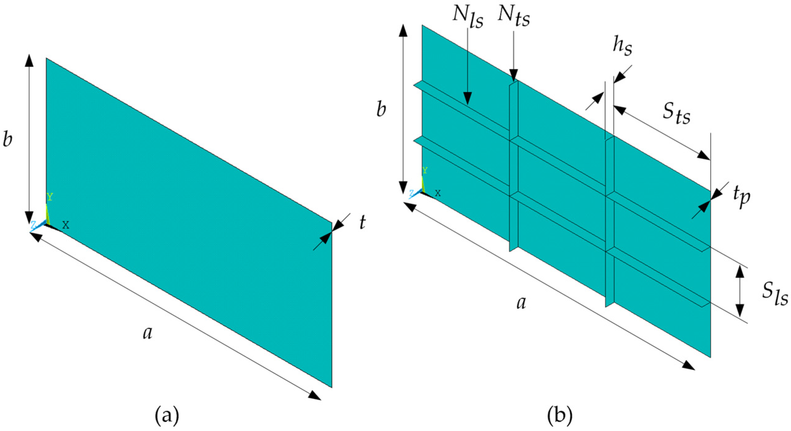
2.2. Computational Modeling of Plates

For the unstiffened plate, the relevant material properties are the module of elasticity E, Poisson’s ratio $\nu$, and the yield stress ${\sigma }_y$; while the geometric parameters are the length a, width b, thickness t, and volume $V_p$ (Figure 1a). For the stiffened plate, the material properties and geometric parameters of the plate remain unchanged, except for the nomenclature of the plate thickness, which is denoted as $t_s$ instead of t. For the stiffeners, the relevant mechanical properties are also E, $\nu$, and ${\sigma }_y$, but some additional dimensions are needed: height $h_s$, thickness $t_s$, height-to-thickness ratio $h_s/t_s$, number of longitudinal stiffeners $N_{ls}$, longitudinal stiffeners spacing $S_{ls}$, number of transverse stiffeners $N_{ts}$, transverse stiffeners spacing $S_{ts}$, and stiffeners volume $V_s$ (Figure 1b). The length of the longitudinal stiffeners is the same as the plate, a, while the length of the transverse stiffeners is equal to the width of the plate, b.

For the case study, the thickness offset of the SHELL281 finite element was the bottom one, which causes the plate’s behavior to exhibit compressive stress and maximum $U_z$ in the positive direction of the z axis, similarly to what occurs in the bottom plates of vessels during sagging, as illustrated by Wang et al. [10], as shown in Figure 2. Due to the selection of the bottom thickness offset, the height $h_s$ of all stiffeners was increased by the value $t_p$ to compensate for the overlap of the plate and stiffeners interface.

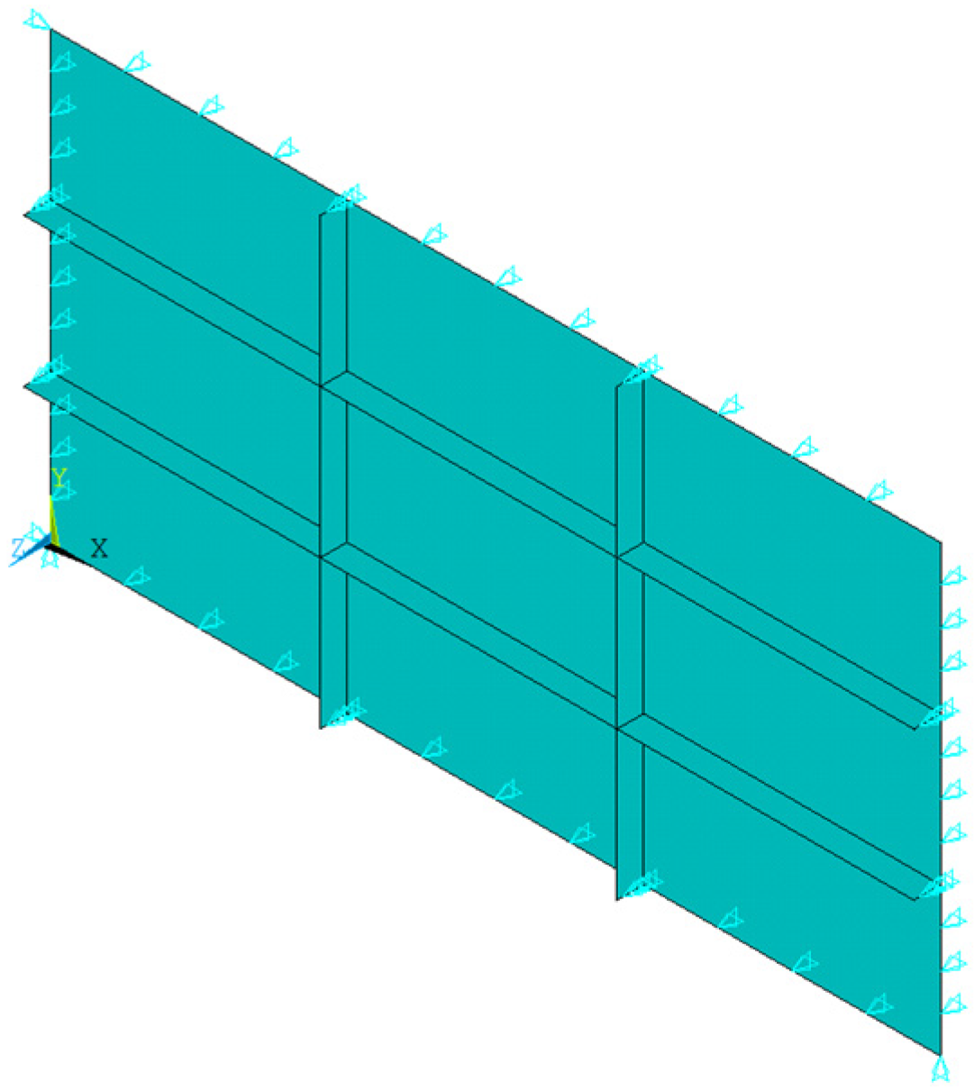
2.2.1. Boundary Conditions

The stiffened plates used in constructing ship’s hull are welded to adjacent sheets and stiffeners, being considered fixed in the boundary. However, representing the plate as simply supported results in a more conservative analysis of the plates’ buckling resistance [19,22]. For this reason, all simulations consider simply supported plates, restricting out-of-plane displacements $U_z$ along all the edges of the plate and stiffeners. Additionally, restrictions on both horizontal $U_x$ and vertical $U_y$ displacements are also applied, as shown in Figure 3.

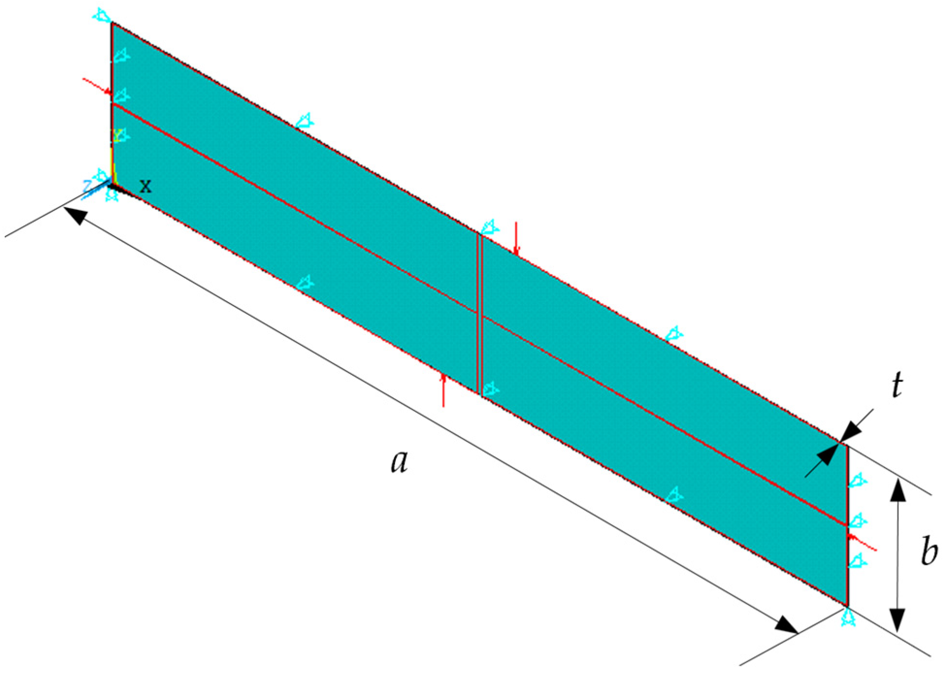
2.2.2. Loading Application

For the case study, only horizontal $P_x$ and vertical $P_y$ in plane loadings were applied to the elastic buckling analysis. In the elastoplastic buckling analysis were applied the combined loading, which includes the $P_x$, $P_y$, and lateral pressure $P_z$. The values of $P_x$ and $P_y$ were the reference loading (Equations (9) and (10)), and the $P_z$ module was constant and equal to 0.16 MPa, representing the extreme pressure conditions projected for a 100,000-ton class double-hull oil tanker [23]. First, the lateral pressure $P_z$ is applied, and large deformations are obtained. After this, $P_z$ is maintained, and biaxial loading is then applied.

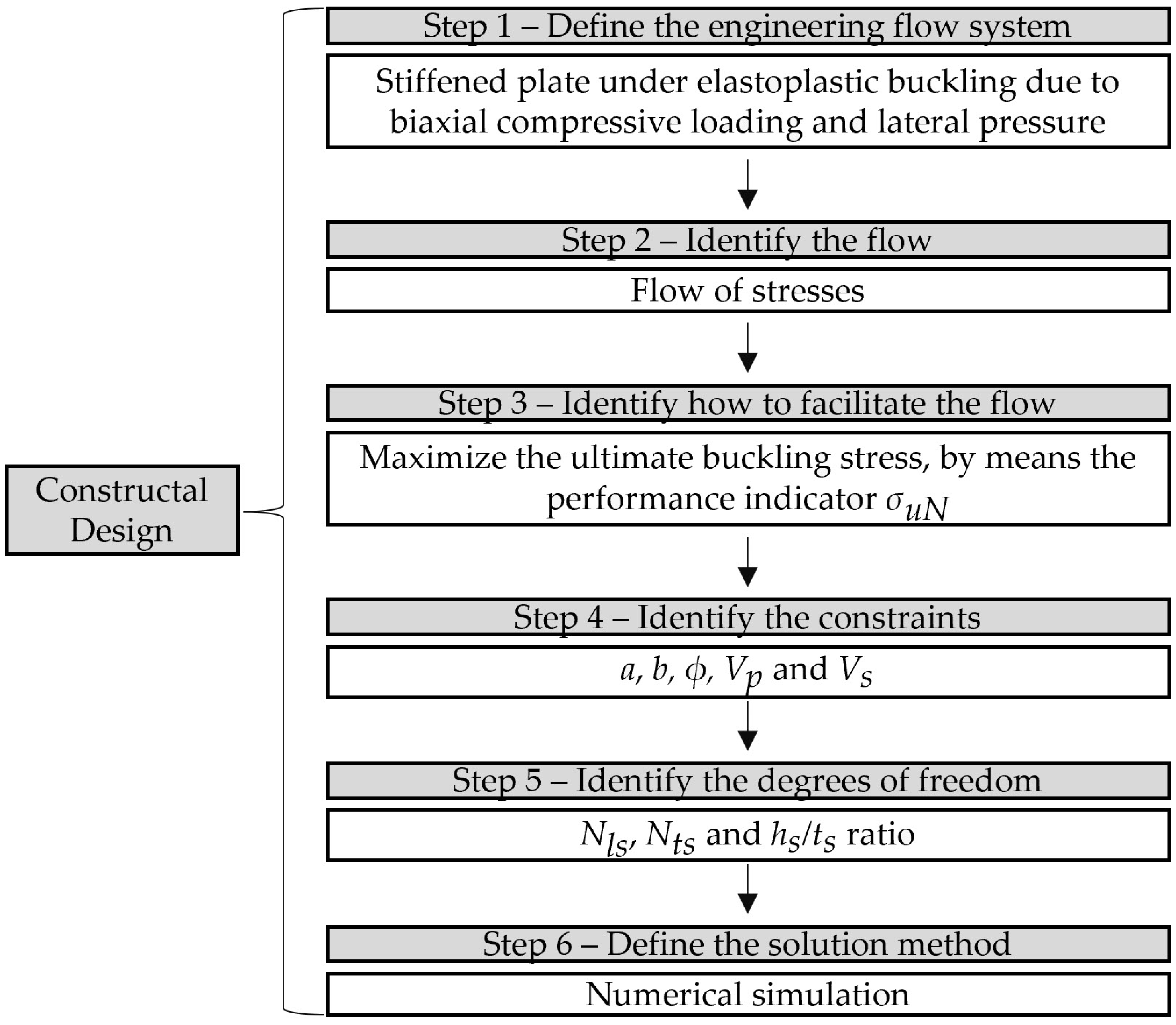
2.3. Constructal Design Method and Exhaustive Search Technique

As in Lima et al. [13], the application of constructal design starts from an unstiffened plate that is considered as a reference, and its ultimate buckling strength ${\sigma }_{uR}$ is adopted as a comparison parameter. The a and b were maintained constantly, and t was reduced to $t_p$ to allocate volume for the stiffeners according to a defined volume fraction $\varphi$, as follows:

$$\varphi ={\displaystyle \frac{V_s}{V_p}}={\displaystyle \frac{N_{ls}(a{h}_s{t}_s)+N_{ts}(b {-{ N}_{ls}t}_s){h_{s}t}_s) }{abt}},$$

(14)

where $\varphi$ represents the fraction of the total volume of the reference plate that is transformed into stiffeners, $V_s$ is the total volume of stiffeners, and $V_p$ is the total volume of the reference plate.

The number of stiffeners $N_{ls}$ and $N_{ts}$ and their respective $h_s$/$t_s$ are degrees of freedom (DOF) necessary for the application of constructal design, generating new geometric configurations of stiffened plates. The ${\sigma }_u$ results of these proposed geometries were obtained and evaluated numerically. It is important to emphasize that the $h_s$ and $t_s$ are variables, but in each new configuration generated, they had the same values for both longitudinal and transverse stiffeners. How ${ N}_{ls}$ and $N_{ts}$ are degrees of freedom, to respect the symmetrical distribution of the stiffeners on the plate, the spacings between stiffeners were defined as:

$$S_{ls}={\displaystyle \frac{b}{N_{ls}+1 }},$$

(15)

$$S_{ts}={\displaystyle \frac{a}{N_{ts}+1 }},$$

(16)

where $S_{ls}$ is the spacing between longitudinal stiffeners and $S_{ts}$ is the spacing between transverse stiffeners.

To understand how the $P_z$ and $h_s$/$t_s$ impacts on ${\sigma }_u$, three conditions of lateral pressure were considered: an application of lateral pressure in a positive direction of the z-axis, in a negative direction of the z-axis, and null pressure. However, the optimized stiffened plate configurations were investigated only for the application of positive lateral pressure and biaxial compressive loading, being the unstiffened plate under this condition defined as the reference plate. This was adopted due to the desirable positive displacement over z-axis, similarly to sagging behavior (Figure 3). Because of this, its respective ultimate buckling stress reference ${\sigma }_{uR}$ was considered for comparisons with the other plate geometries. To compare these results, the ${\sigma }_u$ resulted from geometric configurations proposed by constructal design were dimensionless as normalized ultimate buckling strength ${\sigma }_{uN}$. This serves as the performance indicator, and is calculated as:

$${\sigma }_{uN }={\displaystyle \frac{{\sigma }_u}{{\sigma }_{uR} }},$$

(17)

where ${\sigma }_{uN }$ is the normalized ultimate buckling stress, ${\sigma }_u$ is the ultimate buckling stress obtained from the varying DOF, and ${\sigma }_{uR}$ is the ultimate buckling stress of the reference plate.

In turn, the constructal design method is applied according to the following steps, shown in Figure 4.

The fraction $\varphi$ was set as 0.3, identified by Lima et al. [13] as the best ratio between $V_s$ and $V_p$ to improve ${\sigma }_u$ in elastoplastic buckling due to uniaxial compression, for a plate with the same dimensions considered in this study, with $N_{ls}$ and $N_{ts}$ values ranging from 2 to 5, resulting in sixteen plate configurations. While the $t_s$ was defined as a minimum of 5 mm, set according to commercial dimensions, and varied incrementally up to 45 mm, and the $h_s$ values range depending on the available volume, respecting the volume conservation. This resulted in eight different values of $h_s/t_s$ for each plate configuration, leading to a total of 128 distinct stiffened plates geometries being investigated. As mentioned earlier, due the volume conservation, as $N_{ls}$ and/or $N_{ts}$ increase, the maximum $h_s$ value that the stiffeners can achieve tends to decrease to respect this premise. Moreover, as $t_s$ increases, the $h_s$ value also tends to decrease due to the same principle. This behavior is common to all plate configurations and is illustrated in Figure 5, considering arbitrary $N_{ls}$, $N_{ts},$ and $t_s$ values. Furthermore, the Supplementary Materials provides all the values of $N_{ls}$, $N_{ts}$, $h_s$, and $t_s$, which were determined through the application of constructal design and a graphical explanation of the influence of $N_{ls}$, $N_{ts},$ and $t_s$ over $h_s$.

After that, the exhaustive search technique was applied, according to the subsequent steps shown in Figure 6.

As earlier explained, the number of $N_{ls}$ and $N_{ts}$ ranging from 2 to 5, is allowed to generate sixteen different plate arrangements P($N_{ls};N_{ts}$): P(2;2), P(2;3), P(2;4), P(2;5), P(3;2), P(3;3), P(3;4), P(3;5), P(4;2), P(4;3), P(4;4), P(4;5), P(5;2), P(5;3), P(5;4), and P(5;5). By varying $h_s$/$t_s$ for each arrangement, the optimal stiffened plate geometry was determined to enhance ${\sigma }_{uN}$. All these definitions formed the basis and sequence for the search space used to conduct the exhaustive search technique, as illustrated in Figure 7.

Through the variation of $N_{ls}$, $N_{ts}$, and $h_s$/$t_s$, and calculation of ${\sigma }_{uN}$, the $h_s$/$t_s$ values were identified for each plate configuration that maximized the ${\sigma }_{uN}$. These values were defined as once optimized height-to-thickness ${(h_s/t_s)}_o$ and once maximized ultimate buckling strength ${\left({\sigma }_{uN}\right)}_m$. From these optimized and maximized values, the higher values of ${\left({\sigma }_{uN}\right)}_m$ and consequently their ${(h_s/t_s)}_o$ and $N_{ts}$ were identified and defined as twice maximized ultimate buckling strength ${\left({\sigma }_{uN}\right)}_{mm}$, twice optimized height-to-thickness ratio ${(h_s/t_s)}_{oo}$, and once optimized number of transverse stiffeners ${\left(N_{ts}\right)}_o$. Finally, from these last optimized and maximized values, the plate configuration with the highest ultimate strength was identified, being defined as the three times maximized ultimate strength ${\left({\sigma }_{uN}\right)}_{mmm},$ three times optimized ${(h_s/t_s)}_{ooo}$, twice optimized number of transversal stiffeners ${\left(N_{ts}\right)}_{oo}$, and once optimized number of longitudinal stiffeners ${\left(N_{ls}\right)}_o$.

3. Results and Discussion

3.1. Verification and Validation of Computational Modeling of Buckling

The verification and validation of computational buckling modeling were realized considering the critical and ultimate buckling stress of unstiffened and stiffened plates subjected to axial, biaxial, and combined loadings.

3.1.1. Verification of Elastoplastic Buckling Model Under Combined Loading on Unstiffened Plates

The first verification was carried out considering Paik and Seo [23]’s study, which applied longitudinal compressive loading ${\sigma }_X$ and transverse compressive ${\sigma }_Y$ loading in different ratios, and a constant lateral pressure $P_z$ = 0.16 MPa to a simply supported unstiffened plate, with a = 4300 mm, b = 815 mm, t = 19 mm, E = 208.5 GPa, ${\sigma }_y =$315 MPa, and $\nu =$ 0.3. An initial imperfection of plate as $w_0$ = b/200, while the proposed model considered $w_0$ = b/2000 (Equation (8)). The geometry of the unstiffened plate with boundary conditions of the proposed model is shown in Figure 8.

The finite element size used in the proposed computational modeling was defined according to the mesh convergence test considering the loading condition ${\sigma }_{X }:{\sigma }_Y$ = 0.8:0.2, as shown in

Table 1. Mesh convergence test for verification of elastoplastic buckling model under combined loading on unstiffened plate.

Element Length (mm)	Number of Elements	${\mathbf{\sigma }}_{\mathit{uX}}$ (MPa)
100	387	225.22
75	638	225.22
50	1462	225.22
25	5676	225.22

.

Considering the element size with 25 mm in Table 1, the proposed model resulted in ${\sigma }_{\mathit{uX}}$ = 225.22 MPa and ${\sigma }_{\mathit{uY}}$ = 56.30 MPa. When compared to the values obtained by Paik and Seo [23], which were ${\sigma }_{\mathit{uX}}$ = 222.96 MPa and ${\sigma }_{\mathit{uY}}$ = 55.72 MPa, the differences are 1.01% and 1.04% higher, respectively. For the ratio ${\sigma }_{X }:{\sigma }_Y$ = 0.7:0.3, the proposed model resulted in ${\sigma }_{\mathit{uX}}$ = 159.07 MPa and ${\sigma }_{\mathit{uY}}$ = 68.17 MPa. When compared to the values obtained by Paik and Seo [23] which were ${\sigma }_{\mathit{uX}}$ = 153.97 MPa and ${\sigma }_{\mathit{uY}}$ = 65.99 MPa, the differences are 3.31% and 3.30% higher, respectively. Despite accounting for different boundary conditions and values of initial imperfections, the ultimate stress values confirm that the proposed model is verified for use in the elastoplastic analysis of unstiffened plates.

The second verification was performed considering Baumgardt et al.’s [11] work, which applied biaxial compressive loading and a constant lateral pressure $P_z$ = 0.0507 MPa to a plate made of AH-36 steel, with a = 2000 mm, b = 1000 mm, t = 12 mm, E = 210 GPa, ${\sigma }_y =$355 MPa, and $\nu =$0.3, with a rectangular perforation in the center, with length $a_0=$450 mm and width $b_0=$667 mm, as shown in Figure 9.

Baumgardt et al. [11] used the SHELL281 finite element with 30 mm and a quadrilateral form. The ${\sigma }_u$ obtained with the proposed computational model was achieved according to the mesh convergence test shown in

Table 2. Mesh convergence test for verification of elastoplastic buckling model under combined loading on unstiffened plate with rectangular perforation.

Element Length (mm)	Number of Elements	${\mathbf{\sigma }}_{\mathit{u}}$ (MPa)
100	174	28.75
75	345	28.40
50	704	28.40
30	1974	28.40
25	2747	28.40

.

In the present study, a ${\sigma }_u =$ 28.40 MPa was obtained with 200 sub-steps of loading. When compared to ${\sigma }_u =$ 28.76 MPa with 1000 sub-steps of loading by Baumgardt et al. [11], the result is 1.25% lower. Despite the different reference loading sub-steps considered in each model, the ultimate stress values also confirm that the proposed model is verified for use in the elastoplastic analysis of unstiffened plates.

3.1.2. Verification of Elastoplastic Buckling Model Under Combined Loading on Stiffened Plates

The first verification was developed considering Paik and Seo [24] study, and its results from ANSYS (version 10.0), ALPS/ULSAP (version 2006.3), and DNV PULS (version 2.05) software’s, through the application of longitudinal compressive loading ${\sigma }_X$ and transverse compressive ${\sigma }_Y$ loading in different ratios, and a constant lateral pressure $P_z$ = 0.16 MPa to a simply supported stiffened plate with E = 208.5 GPa, ${\sigma }_y =$315 MPa, $\nu =$0.3, a = 16300 mm, b = 4300 mm, and $t_p$ = 19 mm. The stiffeners present a T-shape, with $t_s$ = 10 mm, $h_s$ = 100 mm, and flange with thickness $t_f=$ 17 mm and height $h_f=$ 172 mm. The initial imperfections were considered as $w_0$ = 4.07 mm from plate, $w_w$ = 0.5 mm for stiffeners web, and $w_f$ = 4.2 mm for fabrication-related initial distortions. The proposed model considered $w_0$ = b/2000 = 2.15 mm (Equation (8)) from the first buckling mode. The geometry of the stiffened plate with boundary conditions of the proposed model is shown in Figure 10.

The finite element size used in the proposed model was defined according to the mesh convergence test considering the loading condition ${\sigma }_X$:${\sigma }_Y$ = 0.79:0.21, presented in

Table 3. Mesh convergence test for verification of elastoplastic buckling model under combined loading on stiffened plates.

Element Length (mm)	Number of Elements	${\mathbf{\sigma }}_{\mathit{u}\mathit{X}}$ (MPa)
600	776	236.25
500	970	236.25
250	4290	236.25

.

The results of ${\sigma }_{\mathit{uX}}$ and ${\sigma }_{\mathit{uY}}$ from the present study and from reference are shown in

Table 4. Results of ${\sigma }_{\mathit{uX}}$ and ${\sigma }_{\mathit{uY}}$ obtained from the present study and from Paik and Seo [24].

${\mathbf{\sigma }}_{\mathit{uX}}:{\mathbf{\sigma }}_{\mathit{uY}}$ Ratio	Present Study		Paik and Seo [24]
			ANSYS		ALPS/ULSAP		DNV PULS
	${\mathbf{\sigma }}_{\mathit{uX}}$	${\mathbf{\sigma }}_{\mathit{uY}}$	${\mathbf{\sigma }}_{\mathit{uX}}$	${\mathbf{\sigma }}_{\mathit{uY}}$	${\mathbf{\sigma }}_{\mathit{uX}}$	${\mathbf{\sigma }}_{\mathit{uY}}$	${\mathbf{\sigma }}_{\mathit{uX}}$	${\mathbf{\sigma }}_{\mathit{uY}}$
0.79:0.21	236.25	62.80	223.65	59.85	199.33	53.55	245.70	66.15
0.40:0.60	76.65	114.97	66.78	100.17	62.02	93.02	73.05	109.56

.

For ${\sigma }_{\mathit{uX}}$:${\sigma }_{\mathit{uY}}$ = 0.79:0.21, the present study achieved ${\sigma }_{\mathit{uX}}$ = 236.25 MPa and ${\sigma }_{\mathit{uY}}$ = 62.80 MPa, showing differences of 5.63% and 4.93% compared to the ANSYS results, 18.52% and 17.27% compared to the ALPS/ULSAP results, and −3.85% and −5.06% compared to the DNV PULS results from Paik and Seo [24]. For the loading condition ${\sigma }_{\mathit{uX}}$:${\sigma }_{\mathit{uY}}$ = 0.40:0.60, the present study resulted in ${\sigma }_{\mathit{uX}}$ = 76.65 MPa and ${\sigma }_{\mathit{uY}}$ = 114.97 MPa, showing, respectively, differences of 14.78% and 14.77% compared to the ANSYS results, 23.59% and 23.60% compared to the ALPS/ULSAP results, and 4.93% and 4.94% compared to the DNV PULS results from Paik and Seo [24]. These differences in results can be attributed to the distinct boundary conditions and the different considerations for initial imperfections between the models. However, the present study demonstrated comparable values with those of Paik and Seo [24].

The second verification of elastoplastic buckling model under combined loading on stiffened plates was carried out based on the study of Beg et al. [25], which presents the $P_u$ through FEM model. Moreover, the ${\sigma }_{cr}$ of this stiffened plate using different solution methodologies (EBPlate (a) and (b), FEM using ABAQUS version 6.7, and the EN1993-1-5 A.2 standard [26]) is also presented in Beg et al. [25], allowing a verification of the proposed elastic buckling model. The studied stiffened plate has material properties of E = 210 GPa, ν = 0.3, and ${\sigma }_y$ = 355 MPa, with dimensions a = 1800 mm, b = 1800 mm, $t_p$ = 12 mm, $t_s$ = 10 mm, and $h_s$ = 100 mm, being submitted to a compressive uniaxial loading, as depicted in Figure 11.

This computational model achieved the ${\sigma }_{cr}$ and $P_u$ through the mesh convergence test, shown in

Table 5. Mesh convergence test for verification of elastic and elastoplastic models of stiffened plate.

Element Length (mm)	Number of Elements	${\mathbf{\sigma }}_{\mathit{cr}}$ (MPa)	${\mathit{P}}_{\mathit{u}}$ (kN)
100	396	277.73	4524.12
75	672	277.76	4524.12
50	1512	277.79	4566.01
25	5904	277.79	4566.01

.

The results obtained are compared with the reference results in

Table 6. Comparison of ${\sigma }_{cr}$ and $P_u$ results between the present study and the referenced literature.

Methodology	${\mathbf{\sigma }}_{\mathit{cr}}$ (MPa)	Difference (%)	Pu (kN)	Difference (%)
Present study	277.76	-	4566.01	-
EBPlate (a)	276.00	0.64	-	-
EBPlate (b)	289.00	−3.89	-	-
ABAQUS	268.00	3.64	4424.00	3.21
EN1993-1-5 A.2 [26]	290.00	−4.22	-	-

.

The present study obtained ${\sigma }_{cr}$ = 277.79 N/mm², showing a small difference when compared to other methods. The maximum difference was 4.22%, which was observed when compared to the EN1993-1-5 A.2 methodology, although with a lower value, providing safety. The smallest difference was obtained in relation to the EBPlate (a) method, with a difference of 0.64% higher. Regarding the finite element method, the difference between the result obtained in this study and the reference using ABAQUS (version 6.7) was 3.64% higher. According to the ultimate strength, the present study results in $P_u$ = 4566.01 kN, 3.11% higher than $P_u$ = 4424.00 kN obtained from FEM by Beg et al. [25]. Overall, the results demonstrate good consistency across the different approaches.

3.1.3. Validation of Elastoplastic Buckling Model Under Combined Loading on Stiffened Plate

The validation was performed by comparing the $P_u$ obtained by the present study with the $P_u$ obtained experimentally by Kumar et al. [26]. The authors applied uniaxial compressive loading and lateral pressure $P_z$ = 0.06 MPa to a stiffened panel, illustrated in Figure 12, having a = 1160 mm, b = 960 mm, $t_p$ = 4 mm, E = 180 GPa, ν = 0.3, and ${\sigma }_{\mathit{yp}} =$ 218 MPa. The panel has four longitudinal stiffeners located with $a_1 =$ 100 mm from the sides and spaced $c_2$ = 320 mm apart, as well as four transverse stiffeners spaced by $b_1$ = 60 mm from the ends and $c_1$ = 280 mm between them. The stiffeners have $t_s$ = 5 mm, $h_s$ = 50 mm, E = 180 GPa, ν = 0.3, and ${\sigma }_{\mathit{ys}}$ = 300 MPa.

For the proposed model, the ${\sigma }_u$ was obtained with the mesh convergence test. The obtained values of ${\sigma }_u$ are presented in

Table 7. Mesh convergence test for validation of ${\sigma }_u$ under combined loading.

Element Length (mm)	Number of Elements	${\mathbf{\sigma }}_{\mathit{u}}$ (MPa)
75	382	140.32
50	894	123.55
35	1472	123.25
20	3936	122.90

.

This model results in ${\sigma }_u$ = 122.90 MPa, with an error of 0.39% compared to the experimental result of ${\sigma }_u$ = 123.38 MPa obtained by Kumar et al. [26]. The displacements and von Mises stress distributions are shown in Figure 13.

The ${\sigma }_u$ obtained for the stiffened panel under combined loading aligns well with the experimental result of Kumar et al. [26]. The transverse stiffeners presented less stress concentration than longitudinal, meaning that the stiffeners in the loading direction are responsible for supporting majority stress, corroborating with Lima et al.’s [13] conclusions about that. Therefore, both quantitatively and qualitatively, the computational model was duly validated.

3.2. Case Study

3.2.1. Mesh Convergence Test

The mesh convergence test was conducted to standardize the mesh element size based on the P(2;2) plate configuration with $h_s$/$t_s$ = 1.02, under $P_z =$ 0.16 MPa and biaxial compression, which were divided into 100 sub-steps. The results of ${\sigma }_u$ are shown in

Table 8. Mesh convergence test for plate configuration P(2;2) with $h_s =$ 45.82 mm and $t_s =$ 45 mm.

Element Length (mm)	Number of Elements	Processing Time (s)	${\mathbf{\sigma }}_{\mathit{u}}$ (MPa)
50	1134	82	101.17
30	3114	112	99.40
25	4140	158	97.62
20	6426	216	97.62
10	24,744	975	97.62

.

From Table 8, one can infer that the mesh convergence test obtained the same ${\sigma }_u$ value for element size with 25 mm, 20 mm, and 10 mm. Considering the element size with 25 mm results in a computational effort reduction by 27% and 84% being achieved, respectively. Moreover, the difference in the von Mises stress distribution is depicted in Figure 14.

Although in some cases the difference in mesh element size does not impact the ${\sigma }_u$, there is a difference in the obtained stress distribution. Therefore, based on Table 8 and Figure 14, the mesh element size adopted for all case studies is 25 mm.

3.2.2. Sub-Steps Convergence Test

The sub-steps convergence test was conducted to standardize the number of sub-steps that the reference loads will be divided and applied. This study is also based on the P(2;2) plate configuration with $h_s$/$t_s$ = 1.02, under $P_z$ = 0.16 MPa and biaxial compression, with a finite element size of 25 mm. The results of ${\sigma }_u$ are shown in

Table 9. Number of sub-steps test for plate configuration P(2;2) with $h_s =$ 45.82 mm and $t_s =$45 mm.

Number of Sub-Steps	Maximum Number of Sub-Steps	Minimum Number of Sub-Steps	Processing Time (s)	${\mathbf{\sigma }}_{\mathit{u}}$ (MPa)
100	200	50	168	97.62
200	400	100	212	98.51
300	600	150	385	98.51
400	800	200	440	98.51

.

The results in Table 9 indicate that dividing the reference load into 100 sub-steps versus 200, 300, and 400 resulted in only a −0.9% difference in ${\sigma }_u$, but reduced computational effort by 21%, 56%, and 62, respectively. In addition, the von Mises stress distribution for each case of Table 9 is presented in Figure 15.

From Figure 15, the stress values and distributions showed a slight discrepancy when considering the different sub-steps. Therefore, to reduce the computational effort, all case study simulations were performed with 100 sub-steps of loading, which can achieve a maximum of 200 and a minimum of 50 sub-steps according to problem convergence.

3.3. Geometric Evaluation

This section presents and discusses the results of the analysis with the constructal design method and exhaustive search technique. To do so, the influence of $P_z$ direction application and degrees of freedom variation on the ultimate biaxial buckling stress of stiffened plates was investigated, allowing to identify the maximized stress and their respective optimized geometric configurations.

3.3.1. Reference Plate

The reference plate was defined as an unstiffened plate with dimensions $a$ = 2000 mm, $b$ = 1000 mm, and $t$ = 20 mm; made of AH-36 steel, with material properties E = 210 GPa, ν = 0.3, and ${\sigma }_y$= 355 MPa; and subjected to a lateral loading $P_z=$0.16 MPa. The application of $P_z$ resulted in an out-of-plane maximum displacement of $U_z=$10.40 mm located at the center of the plate (Figure 16a). Thereafter, with the subsequent application of the biaxial compressive loading, this displacement achieved $U_z =$ 40.19 mm (Figure 16b), resulting in ${\sigma }_{uR} =$44.37 MPa (Figure 16c).

3.3.2. Influence of $P_z$ and $h_s$/$t_s$ over ${\sigma }_{uN}$

Two distinct behaviors from the influence of $P_z$ and $h_s$/$t_s$ over ${\sigma }_{uN}$ were identified in this study: in stiffened plates having $N_{ls}$ < 4 (represented in Figure 17 by stiffened plates $N_{ls}$= 2) and those with $N_{ls}$ ≥ 4 (represented by stiffened plates with $N_{ls}$= 4, which will be presented and discussed later).

In stiffened plates with $N_{ls}$ < 4, from Figure 17, it can be noted that the application of positive lateral pressure reduced the ${\sigma }_{uN}$, while negative lateral pressure increased ${\sigma }_{uN}$. For positive pressure, lower values of $h_s$/$t_s$ resulted in a severe reduction in ${\sigma }_{uN}$. This can be explained by the displacement resulting from the application of positive lateral pressure and subsequent biaxial loading, as illustrated in Figure 18.

In plate configurations with $N_{ls}$< 4, one can observe in Figure 18 that lower values of $h_s$/$t_s$ resulted directly in a global displacements distribution (Figure 18a), and the subsequent application of the biaxial loading maintained this mechanical behavior (Figure 18b), increasing the out-of-plane displacements and leading to a quick structural collapse. On the other hand, higher values of $h_s$/$t_s$ resulted in local displacements distribution due to the application of lateral pressure (Figure 18c). With the subsequent application of biaxial loading, the displacements just evolved until the local collapse of the stiffened plate (Figure 18d). So, in the graphics on Figure 17, at the values of $h_s$/$t_s$ the ${\sigma }_{uN}$ $\mathrm{increased},$ and the stiffened plates geometry results into local displacements until collapse.

Also, for plates configurations with $N_{ls}$< 4, the negative pressure improved ${\sigma }_{uN}$. It can be explained by the displacement resulting from negative lateral pressure and subsequent biaxial loading, shown in Figure 19, in which lower values of $h_s$/$t_s$ resulted in global displacements distribution due to the application of lateral pressure (Figure 19a), and subsequent application of biaxial loading overcame these displacements, resulting in local displacements until collapse (Figure 19b). Higher values of $h_s$/$t_s$ resulted in local displacements due to the application of lateral pressure (Figure 19c), and the subsequent application of biaxial loading also overcame these displacements until the local collapse (Figure 19d). From this reason, there is no significant variation on ${\sigma }_{uN}$ in the graphics in Figure 17, indicating that all $h_s$/$t_s$ values led to local displacements due to the application of biaxial compressive loading until local collapse.

In turn, the results for the stiffened plates with $N_{ls}$ ≥ 4 is presented in Figure 20, represented by the cases with $N_{ls}=$ 4.

It is interesting to emphasize that due to the conservation of the total volume of the stiffened plates (Equation (15)), the increasing number of stiffeners requires reducing the maximum and minimum available $h_s$/$t_s$ values to respect this premise, consequently propitiating global displacements distributions.

In Figure 20, for lower values of $h_s$/$t_s$, the application of positive lateral pressure leads to global displacements distributions, which evolve into global collapse due to compressive biaxial loading, resulting in low values of ${\sigma }_{uN}$ for these geometric configurations. While for higher values of $h_s$/$t_s$, the lateral pressure induces global displacements distributions that evolve into local displacements collapse, resulting in the best ${\sigma }_{uN}$ values for these plate configurations.

Figure 20 also indicates that the negative lateral pressure increased or decreased ${\sigma }_{uN}$ according to $h_s$/$t_s$ values. This fact can be explained by the resulting displacements due to negative lateral pressure application and subsequent biaxial loading, as illustrated in Figure 21.

In Figure 21, one can infer that lower values of $h_s$/$t_s$ led to negative global displacements distributions due to the application of negative $P_z$ (Figure 21a), and the subsequent application of biaxial loading contributed to these negative displacements and consequently considerably reduced ${\sigma }_{uN}$, causing the structural collapse (Figure 21b). Whilst higher values of $h_s$/$t_s$ resulted in negative global displacements distributions due to negative $P_z$ application (Figure 21c), and the subsequent application of biaxial compressive loading resulted in positive displacements (Figure 21d), overcame negative displacements and consequently improved ${\sigma }_{uN}$, collapsing with local displacements (Figure 21b) and achieving better values of ${\sigma }_{uN}$. With this, for negative pressure application (Figure 20), at the $h_s$/$t_s$ as ${\sigma }_{uN}$ presented lower values, the stiffened plate displacements maintained global displacements distributions from negative lateral pressure to biaxial loading until collapse, and the increase of $h_s$/$t_s$ resulted in higher values of ${\sigma }_{uN}$, indicating that the biaxial loading overcame the global displacements into local displacements until collapse.

It could be stated that lower values of $N_{ls}$ allow for higher values of $h_s$/$t_s$, but in contrast, this results in an increased spacing $S_{ls}$ between them, leading to local displacements on the stiffened plate, which tends to improve ${\sigma }_{uN}$. On the other hand, higher values of $N_{ls}$ reduce the spacing $S_{ls}$, but the necessary reduction in $h_s$/$t_s$ to maintain the constant volume constraint makes the stiffened plate more susceptible to global displacement distribution, tending to reduce ${\sigma }_{uN}$.

3.3.3. Highest Values of $h_s$/$t_s$, $N_{ls}$, and $N_{ts}$ over ${\sigma }_{uN}$

The highest value of ${\sigma }_{uN}$ was 3.84, reached from the P(5;4) with $h_s$/$t_s$ = 8.74 and from the P(5;5) with $h_s$/$t_s$ = 8.14, and the P(5;4) selected as better due its lower displacements. The lowest value of ${\sigma }_{uN}$ was 1.22 achieved by P(3;5) with $h_s$/$t_s$ = 0.57. These highest and lowest values represent an increase on ${\sigma }_{uR}$ of 284% and 22%, respectively. The displacement and von Mises stress distributions for both cases are depicted in Figure 22.

The best configuration collapsed with local displacements (Figure 22a), while the worst configuration collapsed with global displacements (Figure 22c). In comparison with their von Mises stress distribution, it noted that the stiffened plate which presented the best stress distribution resulted in the highest ${\sigma }_{uN}$ (Figure 22b). Conversely, the stiffened plate with the worst stress distribution (Figure 22d) displayed the lowest value of ${\sigma }_{uN}$, in accordance with the constructal law.

3.3.4. Influence of $N_{ls}$ and $N_{ts}$ over Once Optimized ${(h_s/t_s)}_o$ and Once Maximized ${\left({\sigma }_{uN}\right)}_m$

From the results of ${\sigma }_{uN}$ for each $h_s/t_s$ value in each plate configuration, the ${\left({\sigma }_{uN}\right)}_m$ and their respective ${(h_s/t_s)}_o$ were obtained, as described in

Table 10. ${\left({\sigma }_{uN}\right)}_m$ and ${(h_s/t_s)}_o$ for plate configurations.

Plate Configuration	Nls	Nts	(hs/ts)o	(σuN)m
P(2;2)	2	2	8.98	3.28
P(2;3)	2	3	7.72	3.36
P(2;4)	2	4	2.46	3.46
P(2;5)	2	5	13.48	3.52
P(3;2)	3	2	15.11	3.56
P(3;3)	3	3	13.47	3.60
P(3;4)	3	4	12.15	3.64
P(3;5)	3	5	11.06	3.68
P(4;2)	4	2	12.10	3.72
P(4;3)	4	3	11.03	3.72
P(4;4)	4	4	10.14	3.76
P(4;5)	4	5	9.38	3.78
P(5;2)	5	2	10.08	3.78
P(5;3)	5	3	9.34	3.80
P(5;4)	5	4	8.70	3.84
P(5;5)	5	5	8.14	3.84

.

Based on the results of Table 10, the highest value of ${\left({\sigma }_{uN}\right)}_m$ was 3.84, achieved by P(5;4) with ${(h_s/t_s)}_o$ = 8.70, while the lowest value of ${\left({\sigma }_{uN}\right)}_m$ was 3.28, reached from the P(2;2) with ${(h_s/t_s)}_o$ = 8.98. These highest and lowest values represent an increase on ${\sigma }_{uR}$ of 284% and 228%, respectively. The displacements and stress distributions are shown in Figure 23, with both P(5;4) and P(2;2) collapsing with local displacements. In comparison with their von Mises stress distribution, it can be noted that the stiffened plate which presented the best stress distribution between plate and stiffeners resulted in the highest ${\left({\sigma }_{uN}\right)}_m$ (Figure 23b), while the stiffened plate that presented the worst stress distribution (Figure 23d) resulted in the lowest ${\left({\sigma }_{uN}\right)}_m$, also respecting the constructal law.

The influence of $N_{ls}$, $N_{ts}$, and ${(h_s/t_s)}_o$ on ${\left({\sigma }_{uN}\right)}_m$ from Table 7 was plotted in Figure 24. The increase in $N_{ls}$ and $N_{ts}$ improved ${\left({\sigma }_{uN}\right)}_m$ and, in general, the ${\left({\sigma }_{uN}\right)}_m$ was obtained by higher values of ${(h_s/t_s)}_o$ from most respective plate configurations, except for plates with P(2;2), P(2;3), and P(2;4). To understand this aspect, the plate configuration P(2;4) served as a model to investigate this behavior through comparison of the resulting displacements and von Mises stress distributions, depicted in Figure 25 and Figure 26 (in which the red color on stiffened plate images represents the maximum values and the blue color represents the minimum values).

Several key findings can be drawn from the behavior of the stiffened plate configurations P(2;2), P(2;3), and P(2;4), as seen in Figure 25 and Figure 26. The ratio $h_s/t_s$ significantly influenced ${\sigma }_{uN}$, with the potential to either improve or reduce the ultimate strength of the stiffened plate. For the highest value $h_s/t_s$ = 6.77 (Figure 25a), the moment of inertia of the stiffeners was so high that it limited their $U_z$ displacements, acting close to dividing the plate into smaller sections. Due to the low number of longitudinal stiffeners, the spacing $S_{ls}$ between them was significant, allowing the plate to displace into areas less influenced by the stiffeners, such as the upper and lower corners. Hence, when lateral pressure and biaxial compressive loading were applied, high displacements occurred at the plate corners, leading to local displacements and collapse. The stress distribution in this case (Figure 26a) showed a poor distribution, with a high concentration of stress only in the plate, ultimately resulting in local collapse.

When $h_s/t_s$ was reduced to 3.83, the moment of inertia of stiffeners decreased, allowing the stiffeners to displace in $U_z$ (Figure 25b). This behavior improved the distribution of displacements across the plate and the stiffeners, including at the upper and lower corners and at the center of the stiffened plate. In addition, ${\sigma }_{uN}$ was not increased with the reduction of $h_s/t_s$ from 6.77 to 3.83, but the geometric configuration resulted in a reduction in maximum local displacements of the plate that also led to local collapse. The stress distribution (Figure 26b) also improved with the reduction of $h_s/t_s$, with a larger area now concentrating the stress more evenly across the plate.

Further reduction of $h_s/t_s$ (Figure 25c) significantly improved the $U_z$ displacement, leading to better displacement distribution between the plate and stiffeners. While the plate still experienced local displacements at the upper and lower corners without failure, local displacements at the center ultimately led to local collapse. The more balanced displacement distribution enhanced the achievement of ${\left({\sigma }_{uN}\right)}_m$ and ${(h_s/t_s)}_o$ for this configuration. Stress distribution (Figure 26c) also improved, with stress concentration previously limited to the plate now also distributed across the transverse stiffeners. This behavior resulted in the plate and stiffeners working together as a cohesive system, achieving the maximum value ${\left({\sigma }_{uN}\right)}_m$ for this case.

Finally, reducing $h_s/t_s$ to the lowest value of 0.78 (Figure 25d) significantly reduced the moment of inertia of the stiffeners, improving $U_z$ in these components and causing them to exhibit the highest displacements. The stiffeners displaced more easily along with the plate, offering minimal resistance to out-of-plane displacements. This behavior resulted in the global displacement distribution of the system, occurring early during lateral pressure application, with displacement continuing as biaxial compression progressed, ultimately leading to global collapse. In contrast to previous configurations, when $h_s/t_s$ was significantly reduced (Figure 26d), the geometry showed the worst stress distribution and ${\sigma }_{uN}$. The transverse stiffeners exhibited a concentration of stress immediately after applying lateral pressure, causing global collapse before any significant stress was distributed across the plate.

3.3.5. Influence of $N_{ls}$, ${\left(N_{ts}\right)}_o$, and ${(h_s/t_s)}_{oo}$ over ${\left({\sigma }_{uN}\right)}_{mm}$

From the results of $N_{ts}$, ${(h_s/t_s)}_o$, and ${\left({\sigma }_{uN}\right)}_m$, the once optimized ${\left(N_{ts}\right)}_o$, the twice maximized normalized ultimate strength ${\left({\sigma }_{uN}\right)}_{mm}$, and their respective twice optimized height-to-thickness ratio ${(h_s/t_s)}_{oo}$ were obtained, as can be viewed in

Table 11. Results of ${\left(N_{ts}\right)}_o$, ${(h_s/t_s)}_{oo}$, and ${\left({\sigma }_{uN}\right)}_{mm}$ for $N_{ls}$.

Plate Configuration	Nls	(Nts)o	(hs/ts)oo	(σuN)mm
P(2;5)	2	5	13.48	3.52
P(3;5)	3	5	11.06	3.68
P(4;5)	4	5	9.38	3.78
P(5;4)	5	4	8.70	3.84

.

The highest value of ${\left({\sigma }_{uN}\right)}_{mm}$ was 3.84, achieved by P(5;4) with ${(h_s/t_s)}_{oo}$ = 8.70, and the lowest value of ${\left({\sigma }_{uN}\right)}_{mm}$ was 3.52, reached from the P(2;5) with ${(h_s/t_s)}_{oo}$ = 13.48. These highest and lowest values represent an increase on ${\sigma }_{uR}$ of 284% and 252%, respectively. The displacements and stress distribution are illustrated in Figure 27.

As previously discussed, the highest value was obtained from P(5;4), which exhibited a geometric configuration that enabled the best distribution of displacements (Figure 27a) and stresses (Figure 27b) between the plate and stiffeners. In contrast, for P(2;5), the lowest value of ${\left({\sigma }_{uN}\right)}_{mm}$ resulted from poor displacement (Figure 27c) and stress distribution (Figure 27d), caused by the very high value of ${(h_s/t_s)}_{oo}$. This behavior led to the highest moment of inertia, which restricted $U_z$ displacements of stiffeners and acted close to dividing the plate into smaller sections. Additionally, the low number of $N_{ls}$ increased the spacing $S_{ls}$ between them. As a result, displacements and stresses became concentrated in areas with less contact with the stiffeners, specifically the upper and lower corners of the plate, with no significant stresses in the stiffeners, leading to a local collapse.

The influence of $N_{ls}$, ${\left(N_{ts}\right)}_o$, and ${(h_s/t_s)}_{oo}$, over ${\left({\sigma }_{uN}\right)}_{mm}$ are graphically shown in Figure 28.

From Figure 28, the plate configurations that had ${\left({\sigma }_{uN}\right)}_{mm}$ presented in majority, the highest value of ${\left(N_{ts}\right)}_o$ for each $N_{ls}$. Only the plate P(5;4) presented less value of ${\left(N_{ts}\right)}_o$, but as discussed previously, both P(5;5) and P(5;4) presented the same value of ${\left({\sigma }_{uN}\right)}_m$, however P(5;4) presented less value of $U_z$, being maximized. Finally, as the increase of $N_{ls}$, the values of ${(h_s/t_s)}_{oo}$ that resulted in ${\left({\sigma }_{uN}\right)}_{mm}$ were the highest from each plate configuration.

4. Conclusions

Through the verification and validation of a numerical model capable of performing elastoplastic analyses of unstiffened and stiffened plates under combined loading, consisting of biaxial compression and lateral pressure, it was possible to apply the constructal design and exhaustive search to understand insights into the elastoplastic buckling behavior. The computational model was verified and validated, respectively, achieving a difference of 3.64% compared to another numerical model and a maximum error of 1.57% compared to the experimental reference. Thereafter, by converting part of the reference plate volume into stiffener volume, all proposed geometric configurations increased ${\sigma }_{uN}$. The geometry that showed the maximized normalized ultimate buckling stress was P(5;4), with ${\left({\sigma }_{uN}\right)}_{mmm}$= 3.84, ${(h_s/t_s)}_{ooo}$= 8.70, ${\left(N_{ts}\right)}_{oo}=$4, and ${\left(N_{ls}\right)}_o=5,$ representing a 284% improvement compared to ${\sigma }_{uR}$ of the unstiffened plated adopted as the reference. In addition, the optimized stiffened plate geometry was 262% superior to the worst stiffened plate geometry P(5;3), with ${\sigma }_{uN}$ = 1.22 and $h_s$/$t_s$= 0.57.

Several relevant conclusions were drawn from this work. The mesh element size and the number of sub-steps in the load application slightly affect the ultimate strength, displacements, and stress distribution of the plates. The application of lateral pressure opposite to the displacement due to biaxial compression can increase buckling resistance by helping to prevent displacements or decrease buckling resistance adding displacements. Converting part of the plate volume into stiffeners can increase the ultimate buckling strength, but it is necessary to determine a better geometric configuration to achieve the best results. The $N_{ls},N_{ts}, \mathrm{and} h_s$/$t_s$ ratio directly affects the displacements caused by lateral pressure and biaxial compression. Very high $h_s$/$t_s$ values tend to improve the moment of inertia, prevent out-of-plane displacement of the stiffeners, concentrate stresses on the plate, and favor the occurrence of local plate collapse. Conversely, very low $h_s$/$t_s$ values tend to cause the stiffeners to displace out of the plane, resulting in the global collapse of the plate and stiffeners. Therefore, the choice of the $N_{ls}$ and $N_{ts}$, as well as their respective $h_s$/$t_s$, should be made to increase the stiffness of the plate–stiffener system, ensuring that both components work together. This behavior will improve the displacement and stress distribution between the plate and stiffeners, leading to higher plate ultimate strength and reduced displacements.

For future work, it is suggested to apply the developed methodology to investigate the mechanical behavior of various stiffener types, explore different plate a/b aspect ratios, and analyze the effects of cyclic loading, welding, and corrosion, together with combined loadings and how the design can improve the ultimate buckling stress in these conditions.

References

1. Tatsumi, A.; Htoo Ko, H.H.; Fujikubo, M. Ultimate strength of container ships subjected to combined hogging moment and bottom local loads, Part 2: An extension of Smith’s method. Mar. Struct. 2020, 69, 102683. [Google Scholar] [CrossRef]
2. Lee, D.H.; Kee Paik, J. Ultimate strength characteristics of as-built ultra-large containership hull structures under combined vertical bending and torsion. Ships Offshore Struct. 2021, 15 (Suppl. S1), S143–S160. [Google Scholar] [CrossRef]
3. Ozdemir, M.; Ergin, A.; Yanagihara, D.; Tanaka, S.; Yao, T. A new method to estimate ultimate strength of stiffened panels under longitudinal thrust based on analytical formulas. Mar. Struct. 2018, 59, 510–535. [Google Scholar] [CrossRef]
4. Li, D.; Chen, Z.; Chen, X. Numerical investigation on the ultimate strength behavior and assessment of continuous hull plate under combined biaxial cyclic loads and lateral pressure. Mar. Struct. 2023, 89, 103408. [Google Scholar] [CrossRef]
5. Ziemian, R. Guide to Stability Design for Metal Structures, 6th ed.; Wiley: Hoboken, NJ, USA, 2010. [Google Scholar]
6. Zhang, D.; Xu, Z.; Okada, T.; Kawamura, Y.; Hayakawa, G.; Ishibashi, K.; Koyama, H. A study on the scantling formulae of a stiffener against lateral pressure under the simultaneous action of axial load. Mar. Struct. 2024, 95, 103595. [Google Scholar] [CrossRef]
7. Reis, A.H. Constructal theory: From engineering to physics, and how flow systems develop shape and structure. Appl. Mech. Rev. 2006, 59, 269–282. [Google Scholar] [CrossRef]
8. Bejan, A. Constructal-theory network of conducting paths for cooling a heat generating volume. Int. J. Heat Mass Transf. 1997, 40, 799–816. [Google Scholar] [CrossRef]
9. Da Silveira, T.; Pinto, V.T.; Lima, J.P.S.; Pavlovic, A.; Rocha, L.A.O.; Dos Santos, E.D.; Isoldi, L.A. Applicability Evidence of Constructal Design in Structural Engineering: Case Study of Biaxial Elasto-Plastic Buckling of Square Steel Plates with Elliptical Cutout. J. Appl. Comput. Mech. 2021, 7, 922–934. [Google Scholar]
10. Wang, Z.; Kong, X.; Wu, W.; Kim, D.K. An advanced design diagram of stiffened plate subjected to combined in-plane and lateral loads considering initial deflection effects. Thin-Walled Struct. 2024, 203, 112144. [Google Scholar] [CrossRef]
11. Baumgardt, G.R.; Fragassa, C.; Rocha, L.A.O.; Dos Santos, E.D.; Da Silveira, T.; Isoldi, L.A. Computational Model Verification and Validation of Elastoplastic Buckling Due to Combined Loads of Thin Plates. Metals 2023, 13, 731. [Google Scholar] [CrossRef]
12. Ma, H.; Xiong, Q.; Wang, D. Experimental and numerical study on the ultimate strength of stiffened plates subjected to combined biaxial compression and lateral loads. Ocean Eng. 2021, 228, 108928. [Google Scholar] [CrossRef]
13. Lima, J.P.S.; Cunha, M.L.; dos Santos, E.D.; Rocha, L.A.O.; Real, M.V.; Isoldi, L.A. Constructal Design for the ultimate buckling stress improvement of stiffened plates submitted to uniaxial compressive load. Eng. Struct. 2020, 203, 109883. [Google Scholar] [CrossRef]
14. Amaral, R.R.; Troina, G.S.; Fragassa, C.; Pavlovic, A.; Cunha, M.L.; Rocha, L.A.O.; dos Santos, E.D.; Isoldi, L.A. Constructal design method dealing with stiffened plates and symmetry boundaries. Theor. Appl. Mech. Lett. 2020, 10, 366–376. [Google Scholar] [CrossRef]
15. Liu, H.; Ong, Y.S.; Cai, J. A survey of adaptive sampling for global metamodeling in support of simulation-based complex engineering design. Struct. Multidiscip. Optim. 2018, 57, 393–416. [Google Scholar] [CrossRef]
16. Amouzgar, K.; Strömberg, N. Radial basis functions as surrogate models with a priori bias in comparison with a posteriori bias. Struct. Multidiscip. Optim. 2017, 55, 1453–1469. [Google Scholar] [CrossRef]
17. Wang, C.M.; Wang, C.Y.; Reddy, J.N. Exact Solutions for Buckling of Structural Members. In CRC Series in Computational Mechanics and Applied Analysis; CRC Press: Boca Raton, FL, USA, 2004. [Google Scholar] [CrossRef]
18. Przemieniecki. Theory of Matrix Structural Analysis; Dover Publications: Mineola, NY, USA, 1985. [Google Scholar]
19. El-Sawy, K.M.; Nazmy, A.S.; Martini, M.I. Elasto-plastic buckling of perforated plates under uniaxial compression. Thin-Walled Struct. 2004, 42, 1083–1101. [Google Scholar] [CrossRef]
20. Fonseca, E.M.M. Steel Columns under Compression with Different Sizes of Square Hollow Cross-Sections, Lengths, and End Constraints. Appl. Sci. 2024, 14, 8668. [Google Scholar] [CrossRef]
21. ANSYS Inc. Element reference. In Ansys Mechanical APDL Manual; ANSYS Inc.: Canonsburg, PA, USA, 2011. [Google Scholar]
22. Kim, J.H.; Jeon, J.H.; Park, J.S.; Seo, H.D.; Ahn, H.J.; Lee, J.M. Effect of reinforcement on buckling and ultimate strength of perforated plates. Int. J. Mech. Sci. 2015, 92, 194–205. [Google Scholar] [CrossRef]
23. Paik, J.K.; Kim, B.J.; Seo, J.K. Methods for ultimate limit state assessment of ships and ship-shaped offshore structures: Part I-Unstiffened plates. Ocean Eng. 2008, 35, 261–270. [Google Scholar] [CrossRef]
24. Paik, J.K.; Kim, B.J.; Seo, J.K. Methods for ultimate limit state assessment of ships and ship-shaped offshore structures: Part II-Stiffened plates. Ocean Eng. 2008, 35, 271–280. [Google Scholar] [CrossRef]
25. Beg, D.; Kuhlmann, U.; Davaine, L.; Braun, B. Design of plated structures: Eurocode 3: Design of steel structures. Part 1–5, design of plated structures. In ECCS—European Convention for Constructional Steelwork; John Wiley & Sons: Hoboken, NJ, USA, 2010. [Google Scholar]
26. Suneel Kumar, M.; Lavana Kumar, C.; Alagusundaramoorthy, P.; Sundaravadivelu, R. Ultimate strength of orthogonal stiffened plates subjected to axial and lateral loads. J. Civ. Eng. 2010, 14, 197–206. [Google Scholar]
Figure 1. Computational modeling of: (a) unstiffened plate and (b) stiffened plate.
Applsci 15 03354 g001
Figure 2. Behavior of vessel plates loading and deformations in sagging and hogging conditions (adapted from Wang et al. [10]), being the cargo weight the total weight that the ship is transporting and the continuous blue line the waterline.
Applsci 15 03354 g002
Figure 3. Boundary conditions of a simply supported stiffened plate, with displacement restrictions represented in blue on the stiffened plate boards, according to the respective axis directions.
Applsci 15 03354 g003
Figure 4. Steps of constructal design method (adapted from Lima et al. [13]).
Applsci 15 03354 g004
Figure 5. Influence of N l s , N t s , and t s over h s : (a) P(2;2), (b) P(2;4), and (c) P(3;5).
Applsci 15 03354 g005
Figure 6. Steps of exhaustive search technique (adapted from Lima et al. [13]).
Applsci 15 03354 g006
Figure 7. Search space sequence for exhaustive search technique application (adapted from Lima et al. [13]).
Applsci 15 03354 g007
Figure 8. Unstiffened plate geometry and boundary conditions of the proposed model, with the blue symbols representing the displacement constraints according to the axis direction, the red arrows representing the biaxial compressive loading, and the red lines on the plate representing the applied lateral pressure.
Applsci 15 03354 g008
Figure 9. Unstiffened plate geometry with rectangular hole and boundary conditions of the proposed model, with the blue symbols representing the displacement constraints according to the axis direction, the red arrows representing the biaxial compressive loading, and the red lines on the plate representing the applied lateral pressure.
Applsci 15 03354 g009
Figure 10. Stiffened plate: (a) geometry and (b) boundary conditions of the proposed model, with the blue symbols representing the displacement constraints according to the axis direction, the red arrows representing the biaxial compressive loading, and the red lines on the plate representing the applied lateral pressure.
Applsci 15 03354 g010
Figure 11. Modeling of plate with two longitudinal stiffeners, with the blue symbols representing the displacement constraints according to the axis direction and the red arrows representing the uniaxial compressive loading.
Applsci 15 03354 g011
Figure 12. Stiffened plate considered in validation: (a) dimensions and (b) loading and boundary conditions, with the blue symbols representing the displacement constraints according to the axis direction, the red arrows representing the biaxial compressive loading, and the red lines on the plate representing the applied lateral pressure.
Applsci 15 03354 g012
Figure 13. Validation of elastoplastic buckling of stiffened plates due combined loading: (a) U z and (b) von Mises stress distribution.
Applsci 15 03354 g013
Figure 14. The von Mises stress distribution of plates with finite element size of: (a) 50 mm, (b) 30 mm, (c) 25 mm, (d) 20 mm, and (e) 10 mm.
Applsci 15 03354 g014
Figure 15. The von Mises stress distribution of plates with number of sub-steps: (a) 100, (b) 200, (c) 300, and (d) 400.
Applsci 15 03354 g015
Figure 16. Unstiffened plate with application of P z   =   0.16 MPa: (a) U z due lateral pressure, (b) U z due application of lateral pressure and biaxial compression, and (c) von Mises stress distribution due application of lateral pressure and biaxial compression.
Applsci 15 03354 g016
Figure 17. Influence of h s / t s and lateral pressure P z on σ u N in plates with N l s   < 4: (a) P(2;2), (b) P(2;3), (c) P(2;4), and (d) P(2;5).
Applsci 15 03354 g017
Figure 18. Influence of h s / t s , positive lateral pressure, and subsequent biaxial compressive loading on displacements of plates with N l s   < 4: (a) h s / t s = 1.02 and lateral pressure, (b) h s / t s = 1.02, lateral pressure, and biaxial loading, (c) h s / t s = 20.13 and lateral pressure, and (d) h s / t s = 20.13, lateral pressure, and biaxial loading.
Applsci 15 03354 g018
Figure 19. Influence of h s / t s , negative lateral pressure, and subsequent biaxial compressive loading on displacements of plates with N l s < 4: (a) h s / t s = 1.02 and lateral pressure, (b) h s / t s = 1.02, lateral pressure, and biaxial loading, (c) h s / t s = 20.13 and lateral pressure, and (d) h s / t s = 20.13, lateral pressure, and biaxial loading.
Applsci 15 03354 g019
Figure 20. Influence of h s / t s and lateral pressure on σ u N in plates with N l s ≥ 4: (a) P(4;2), (b) P(4;3), (c) P(4;4), and (d) P(4;5).
Applsci 15 03354 g020
Figure 21. Influence of h s / t s , negative lateral pressure, and subsequent biaxial compressive loading on displacements of plates with N l s ≥ 4: (a) h s / t s = 0.61 and negative lateral pressure, (b) h s / t s = 0.61, negative lateral pressure, and biaxial loading, (c) h s / t s = 12.10 and lateral pressure, and (d) h s / t s = 12.10, negative lateral pressure, and biaxial loading.
Applsci 15 03354 g021
Figure 22. Best and worst plate configurations displacements and von Mises stress distribution: (a) P(5;4) displacements, (b) P(5;4) stress distribution, (c) P(3;5) displacements, and (d) P(3;5) stress distribution.
Applsci 15 03354 g022
Figure 23. Displacements and von Mises stress distribution of best and worst plate configurations on ( σ u N ) m : (a) P(5;4) displacements, (b) P(5;4) stress distribution, (c) P(2;2) displacements, and (d) P(2;2) stress distribution.
Applsci 15 03354 g023
Figure 24. Influence of N l s and N t s on: (a) ( σ u N ) m and (b) ( h s / t s ) o .
Applsci 15 03354 g024
Figure 25. Results of the application of lateral pressure and subsequent compressive biaxial loading on displacements of P(2;4) with different values of h s / t s : (a) h s / t s = 6.77, (b) h s / t s = 3.83, (c) h s / t s = 2.46, and (d) h s / t s = 0.78.
Applsci 15 03354 g025
Figure 26. Results of the application of lateral pressure and subsequent biaxial compressive loading on von Mises stress of P(2;4) with different values of h s / t s : (a) h s / t s = 6.77, (b) h s / t s = 3.83, (c) h s / t s = 2.46, and (d) h s / t s = 0.78.
Applsci 15 03354 g026
Figure 27. Displacements and von Mises stress distribution of best and worst plate configurations on σ u N m m : (a) P(5;4) displacements, (b) P(5;4) stress distribution, (c) P(2;5) displacements, and (d) P(2;5) stress distribution.
Applsci 15 03354 g027
Figure 28. Influence of N l s over ( N t s ) o , ( h s / t s ) o o , and ( σ u N ) m m .
Applsci 15 03354 g028