Evaluating the Degradation of WE43 for Implant Applications: Optical and Mechanical Insights

Featured Application

Basic investigation of the use of magnesium alloy WE43 as an orthopaedic implant.

Abstract

In the context of an ageing society, advancements in medicine and biomedical technology are becoming increasingly important. A major goal is to minimise the number of surgical operations. Magnesium alloys are gaining attention due to their degradable properties, good biocompatibility, and osteoconductivity. However, for implants made from this material to be usable, a precise understanding of the degradation rate and a correspondingly adapted design must be available. This work focuses on constructing a suitable experimental chamber for degradation analysis, as well as investigating the impact of sample positioning on degradation using two different geometries of WE43 alloy for potential use as osteosynthesis implants. Optical and mechanical tests were carried out on these geometries. The tests revealed that the sample positioning in the experimental chamber affects degradation, with the central position yielding the most suitable results for future applications. In addition, mechanical tests demonstrated reduced mechanical properties in the degradation layer. This work provides an initial basis for further investigations into the use of the WE43 alloy as an osteosynthesis implant and supports the numerical calculation of degradation.

1. Introduction

Due to an ageing society, medicine and biomedical technology are facing new challenges. These include an increasing number of operations, which relate to orthopaedic care and consequently a higher risk of side effects or subsequent illnesses [1]. In the field of implantology, in particular, the orthopaedic treatment of deformities or fractures, metallic materials are frequently applied. The natural regeneration process in cases of patient fractures or deformities is facilitated through the use of these implants. Implants can be differentiated into permanent and temporary implants [2]. The latter have a significant benefit in the application and are further differentiated into temporarily non-resorbable and temporarily resorbable implants. Temporarily resorbable implants eliminate the need for a second operation to remove the implant [3]. As regards temporarily resorbable materials, options include degradable metallic materials such as magnesium, as well as polymers, composite materials, and bioceramics. Materials are chosen based on the area of application and the specific objective, making different groups of the listed materials appropriate [4]. In addition to the necessary mechanical properties, these materials are subject to extensive requirements with regard to their biocompatibility. From a fundamental point of view, all elements present in the implant material are released into the organism during degradation. Therefore, it must be ensured that this does not have any negative side effects on the human body [5]. According to Wintermantel et al., biocompatibility is described as the compatibility between a technical and a biological system, whereby no toxic or allergic reactions are caused [2].

The focus of this work is on magnesium alloys, as pure magnesium is unsuitable for use in medical technology due to its high degradation rate [6]. Due to their special material properties, such as biocompatibility or stimulation of bone growth (osteoconductivity), these alloys are increasingly becoming the focus of research questions. In the field of implantology, these alloys are also attractive due to their ability to dissolve in the body (degradation) and to be decomposed [3]. Based on numerous in vivo studies, magnesium and its alloys have been found to be a resorbable material with great biocompatibility [7,8,9]. Moreover, orthopaedic implants made of magnesium alloys have been shown to have a positive effect on new bone tissue and blood vessel formation [10]. For instance, the suitability of magnesium for use as a screw has been evaluated both numerically and through simplified experimental trials, and it has been identified as feasible [11]. Therefore, magnesium alloys could be widely used for orthopaedic purposes [12].

For the application as implant materials, the materials must be analysed through degradation experiments. Consequently, various degradation test setups have been developed, each study emphasising a different aspect; however, a dedicated setup specifically for osteosynthesis implants has not yet been established. In this work, the magnesium alloy WE43 was investigated in greater detail for its potential use as an orthopaedic implant in a body replacement fluid. To provide an initial assessment, an appropriate degradation setup was established, which continuously recorded parameters such as temperature and pH value throughout the experiment’s duration. Within this setup, three different positions were evaluated for their suitability as sample sites. The experiments were analysed in terms of surface roughness and prevailing flow conditions. Additionally, the effect of two different sample geometries on degradation was investigated. The results were evaluated in terms of degradation phenomena and degradation rates and assessed for their suitability as osteosynthesis implants. To further assess the applicability in this area, the mechanical properties of the degradation layer were determined and compared with the base material.

2. State of the Art

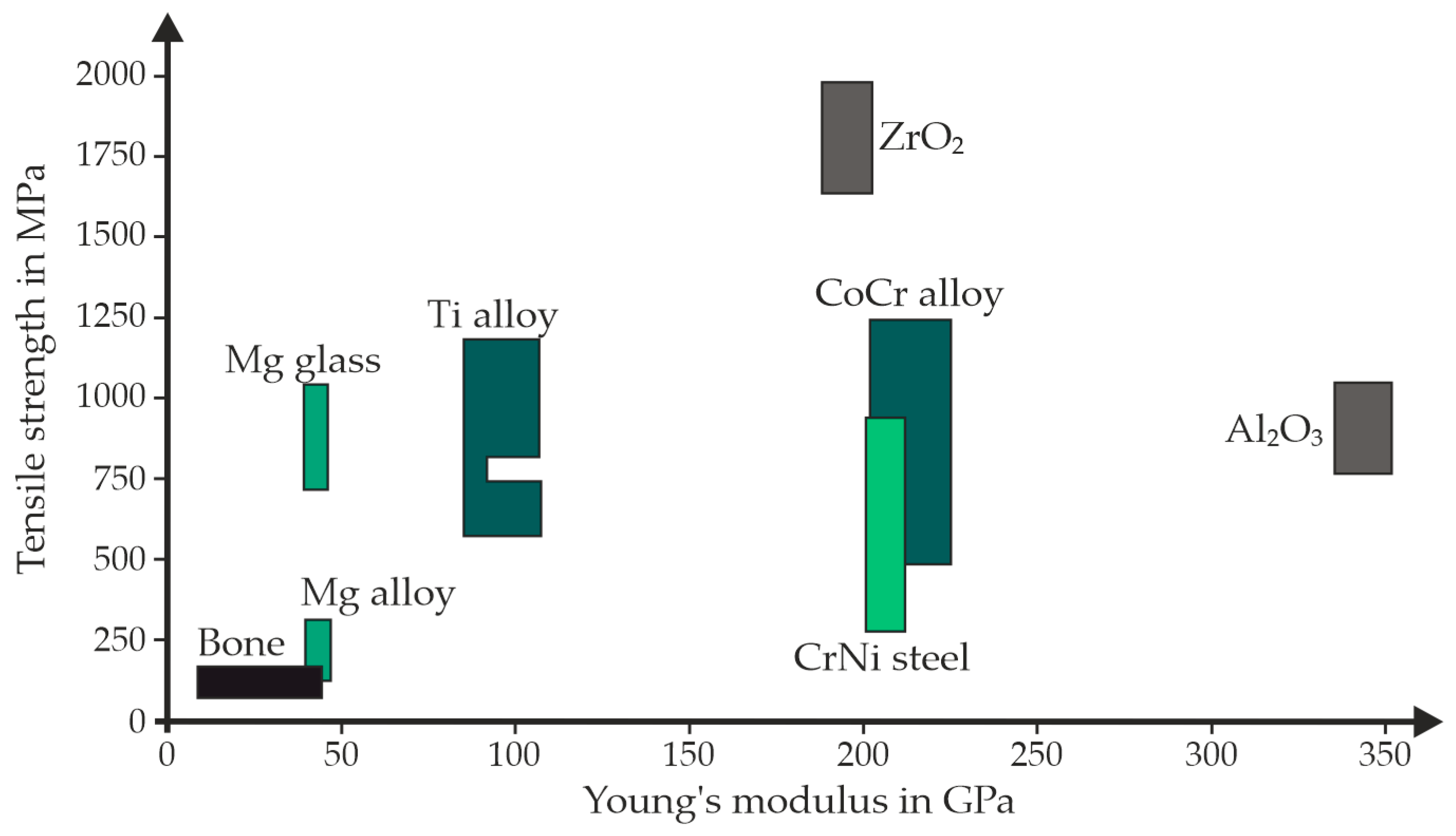
2.1. Classification of Magnesium and Its Alloys

Current metallic implants predominantly consist of a titanium alloy or a CoCr-alloy, which has at least three times the Young’s modulus and five to ten times the tensile strength compared to human bone (Figure 1) [13]. Due to the higher mechanical properties, stress shielding occurs when these materials are used as load-bearing implant materials. Efforts are being made to avoid this process. This can be achieved, for example, by choosing a different material. As a result, magnesium alloys are increasingly becoming the focus of research questions. Using magnesium alloys, the stress shielding of the bone is reduced and better healing of the bone is achieved [4].

The group of magnesium alloys also includes the alloy WE43 [14,15]. WE43 is approved for medical use and, in terms of mechanical properties and regulatory approval as a medical implant, is comparable to the magnesium screws commercially distributed by Syntellix [12]. In addition, this alloy has a similar density to bone, as shown in

Table 1. Individual mechanical properties of human bone, pure magnesium, and magnesium alloy WE43 [14,16].

Material	Density in g/cm3	Tensile Strength in MPa	Young’s Modulus in GPa
Average human bone	1.80–2.10	110–130	10–30
Pure magnesium	1.74–2.00	90–190	41–45
WE43	1.83–1.84	~220	~44

. Regarding tensile strength and Young’s modulus, the values are above those of human bone and partially above those of pure magnesium [13].

In addition to the mechanical properties, other characteristics like biocompatibility or manufacturability are also important for an implant material. During the degradation of magnesium alloys in aqueous solutions, including physiological fluids such as body replacement fluid, magnesium dissolves. As a result of the degradation, magnesium hydroxide (Mg(OH)₂) and hydrogen gas (H₂) are formed (Equation (1)). These degradation products must be manageable by the body. Therefore, it is important to select a degradation rate that aligns with the body’s capacity to process the resultant degradation products [17,18].

$$Mg+2H_{2}O\rightleftharpoons Mg{\left(OH\right)}_2+H_2$$

(1)

In addition to the time required for the removal of degradation products, the loss of mechanical strength due to the degradation process also plays a crucial role in determining the recommended degradation rate [19]. The degradation rate in millimetres per year (mm/y) should be less than 0.5 mm/y and higher than 0.2 mm/y to match the healing rate of the bone and correspond to the body’s capacity to manage the resulting degradation products [20]. The degradation rate can be calculated using Equation (2) [21]. Early degradation can lead to failure of the implant. This, in turn, means that complete healing cannot be guaranteed. This is because the bone has not yet had sufficient time to regain strength and stability and to withstand the loads that occur [22]. The relevance of the required mechanical strength of the bioresorbable implant can be seen by comparing the degradation of the implant and the healing process of the bone in Figure 2. The implanted material should necessarily provide the required load-bearing capacity during the healing process, as it takes over the support function of the bone [23].

$$P_W={\displaystyle \frac{3.65\times ∆W_r}{\rho }}$$

(2)

P_W = degradation rate in mm/y (gravimetric); ΔW_r = mass loss per area and time unit in mg/cm²/d; ρ = density of the sample in g/cm³ [21].

Figure 2. Idealised target degradation rate in relation to bone formation (modified after [10]).

Figure 2. Idealised target degradation rate in relation to bone formation (modified after [10]).

2.2. Degradation Experiments on Magnesium Alloys

Shang et al. developed an experimental test chamber where a dynamic flow state of the body replacement fluid can be set for the abstraction of a blood vessel. The samples are placed within a single tubular section, with a pump installed ahead of it. In addition, the change in the pH value was recorded over the duration of the experiments. The degradation rate is established by assessing the Mg²⁺ concentration using an atomic absorption spectrophotometer [24]. Other approaches for determining the degradation rate are electrochemical measurement using electrochemical impedance spectroscopy or determination of the mass loss by weighting. The same tendencies can be seen in the results, whereby the determination of the weighting cannot be carried out continuously during the decomposition process, but only when the process is interrupted or terminated [25].

The determination of the degradation rate using the mass loss approach (weighing) was compared with the volume loss approach using µCT measurements in the work by Liu et al. Both approaches provide similar results, but the volume loss approach is particularly suitable for very small samples and short degradation times. In addition, the degradation products do not have to be removed with this approach. However, the measurements and data analyses are time-consuming. The mass loss approach (weighing), on the other hand, is faster and can always be performed [6].

A simplified experimental setup for measuring the influence of degradation on the mechanical properties and the degradation form is described in the work of van Gaalen et al. [26]. Here, the degradation rate was determined on the basis of H₂ evolution. For this purpose, a burette was fixed over the sample and the rising gas was collected. To ensure a uniform pH value in the body replacement fluid, a magnetic stirrer was placed at a certain distance below the sample. Parafilm was wrapped around the areas to be protected so that the sample was not exposed to the fluid in all areas [26]. The same approach for establishing fluid circulation was also used by Li et al. [27].

2.3. Magnesium Alloy WE43

The magnesium alloy WE43 is classified among the ternary alloy systems and contains rare earths (

Table 2. Chemical composition of WE43 by weight (%) (yttrium = Y; zirconium = Zr; gadolinium = Gd; neodymium = Nd; copper = Cu; nickel = Ni; iron = Fe; magnesium = Mg) [3,31].

Y	Zr	Gd	Nd	Cu	Ni	Fe	Mg
3.7–4.3	0.4–1.0	0.0–0.9	2.0–2.5	≤0.02	≤0.005	≤0.01	rest

) [3,28]. It is considered biocompatible [29] and has a positive effect on bone growth [13]. As an additional positive effect, the alloy has an infection-inhibiting effect, which makes the material particularly attractive for use as an implant [30].

Van Gaalen et al. used a test rig for the degradation of magnesium WE43 round tensile samples, which were subsequently mechanically tested by means of tensile experiments. Within these tests, four different times (7, 14, 21, and 28 days) of degradation were compared with the initial state. It was established that the strength decreases over the period of degradation. In addition to assessing the mechanical properties at different degradation times, the change in geometry over time was also observed. For this purpose, computer tomography (CT) scans of the samples were taken and the change in depth was analysed. The analysis revealed that the samples exhibited surface corrosion as well as pitting corrosion. Over time, pitting corrosion formed smaller holes that coalesced into larger holes, with a sharp increase in depth observed between day 21 and day 28. In addition, the degradation rate was compared by measuring the H₂ evolution and by determining the volume loss based on the CT scans. The comparison indicated that the determination of the degradation rate using the H₂ evolution method yielded lower results than the method used for assessing volume loss via CT scans [26].

In the study by Windhagen et al., screws made of titanium were compared with MgYREZr (Magnezix^® by Syntellix) screws for the treatment of hallux valgus [32]. The MgYREZr screws exhibited the same mechanical properties as the WE43 alloy. One group of patients was treated with the titanium screw, and the other group received the MgYREZr screw. The titanium screw was considered the gold standard and reference trial. No negative influence of the MgYREZr screw, such as allergic reaction, osteolysis, or foreign body reaction, was observed during the study period. The healing process of both groups was identical and fulfilled their function. These results were confirmed by the work of Klauser and supplemented by the information that normal bone function was present after the healing phase and degradation of the MgYREZr screw [30]. The advantage of the Mg screws was that they did not have to be removed again due to degradation and, therefore, had no negative influence on the patient’s life later on. The presented results were confirmed in the work of Sahin et al. [33]. Titanium and magnesium screws were tested ex vivo in sawbones. The mechanical experiments involved applying a compressive load in two effective directions on the sawbones and the implant. No significant difference was found between the screws in these tests.

3. Materials and Methods

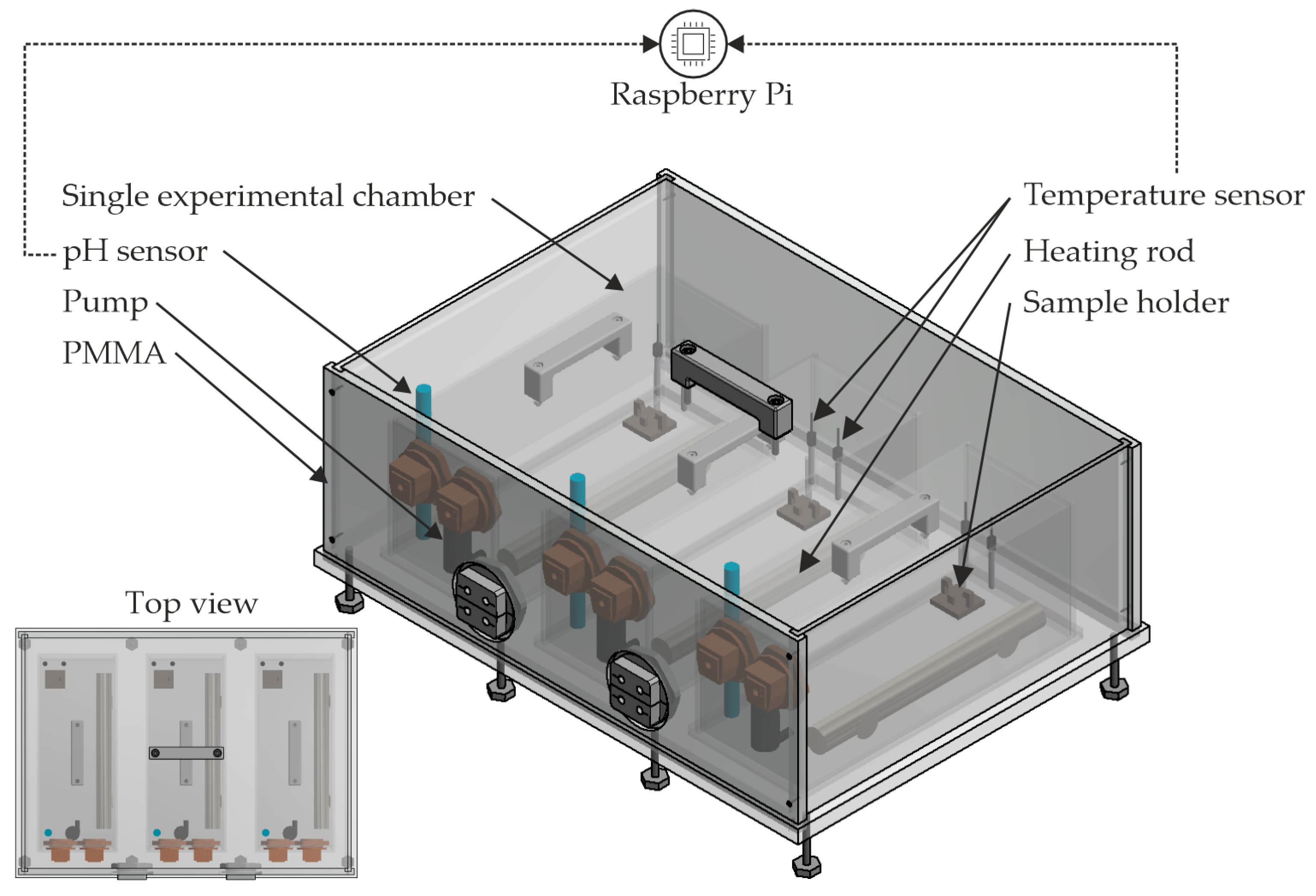
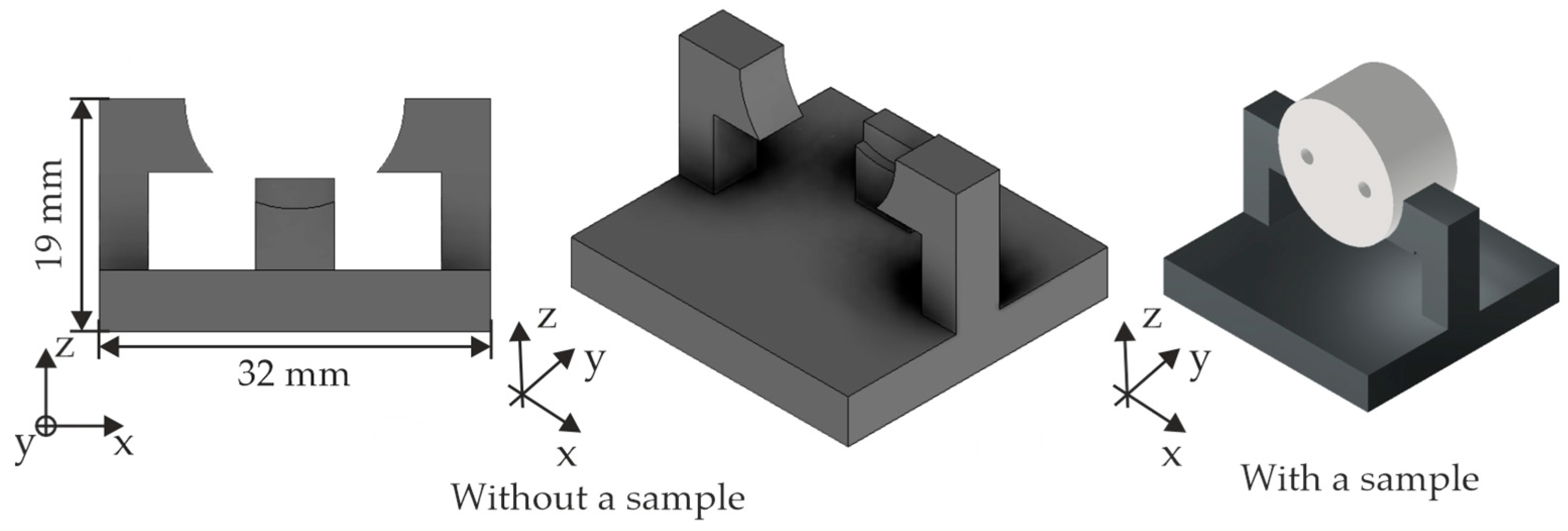
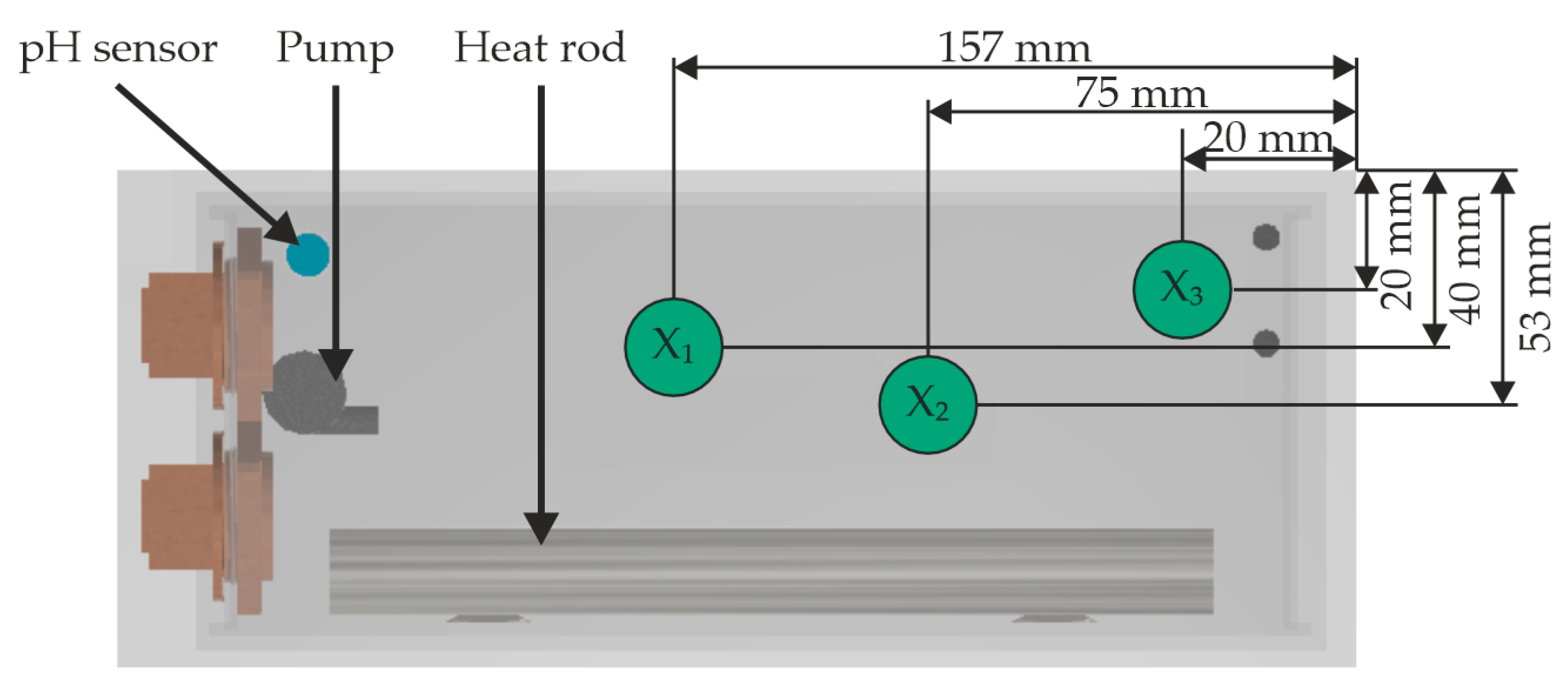
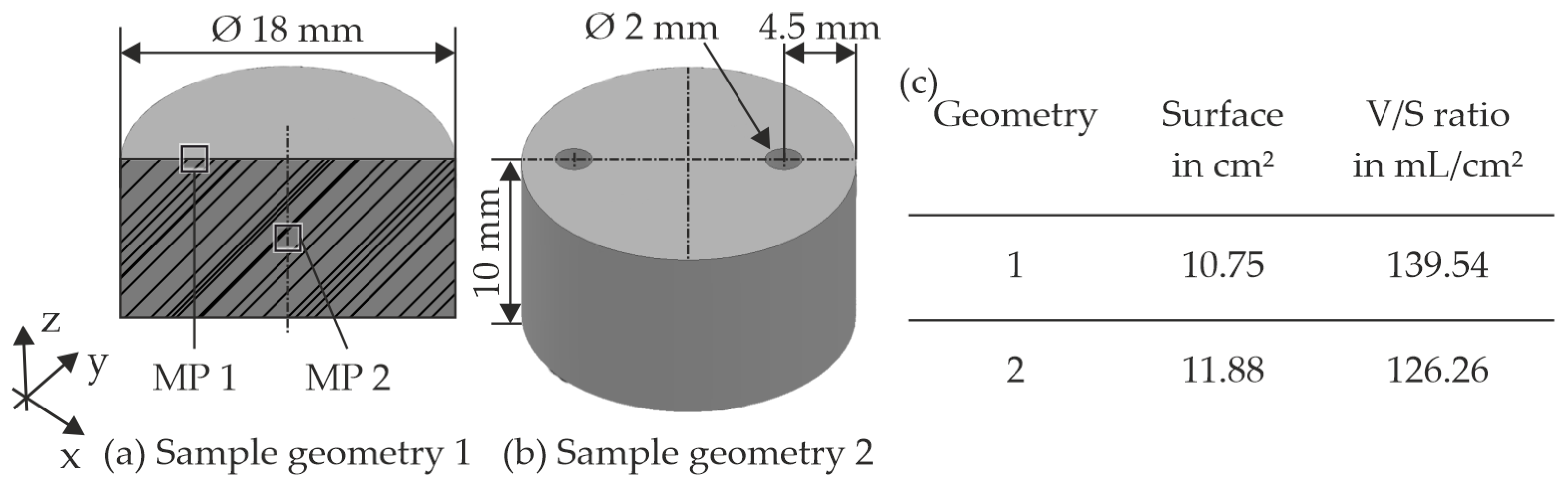
3.1. Experimental Setup and Preparation of the Experiments

An experimental setup was designed and constructed before the experiments were carried out, which is shown schematically in Figure 3. The aim was to have three independently running experimental chambers (three in one box), each with identical but autonomously operating sensor technology. Three experimental chambers were aimed for, allowing multiple independent experiments to be conducted simultaneously. The construction of an immersion test (an experiment to evaluate chemical resistance) [16], which determines mass loss using the gravimetric method [6], was considered to be the most effective in the context of this work. The advantage is that, for example, the gases produced do not have to be collected in an extra container for volume measurement. This ensures that different sample geometries can also be analysed at different locations in the experimental chamber. By using the immersion experiment, it is possible to create a bone-like environment. In this environment, for example, there are no high flow properties as in blood vessels (artery 30–40 cm/s [2]) or high temperature fluctuations as on the skin. Furthermore, it was necessary to implement a flow in the fluid by using pumps. A circulation pump (Micro Centrifugal Liquid Pump Range from TCS Micropumps Ltd, UK) was used to maintain a constant fluid volume, eliminating the need for an additional reservoir. The pumps are each attached to one end of the test chamber with a flow rate of 330 mL/min, based on information provided by the manufacturer (left side in Figure 3). The inlet and outlet of the pump were positioned at the same vertical height to ensure that the flow behaviour was not affected by any additional gravitational influences. In order to simulate the flowing environment, which represents an abstraction for later use as an osteosynthesis implant, a suitable flow was selected. A flow rate was targeted, ranging from a minimum of 7.065 mL/min to 706.5 mL/min, based on typical mid-sized veins due to the lack of available measurements within bones [2]. This enables the simulation on a laboratory scale of the degradation of the implant by the body’s own processes. The sensor technology includes a temperature controller (heating rod from Schego, Schemel & Goetz GmbH & Co KG, Offenbach, Germany), each equipped with its own temperature sensor (Hobby Biotherm, Dohse Aquaristik GmbH & Co. KG, Gelsdorf, Germany), within each experimental chamber. In addition, each experimental chamber has a pH sensor (Gravity compatible with Raspberry Pi (DFRobot, Shanghai, China)) and another temperature sensor (DEBO LK-Temp compatible with Raspberry Pi (Reichelt Elektronik GmbH, Sande, Germany)). These are each connected to the Raspberry Pi for storing the results. The data storage of the Raspberry Pi can be varied and was set to a frequency of 3600 s for longer experiments. The temperature sensors, as well as the pH sensor, are positioned opposite the pump side to effectively monitor temperature and pH value development. Consideration was given to positioning the pH sensor away from the direct exposure outlet to the pump to ensure accurate measurements. Each experimental chamber measures 114 × 296 × 126 mm (width × length × height (w × l × h)) and is made of polymethyl methacrylate (PMMA). The box around the three experimental chambers was made of PMMA with the dimensions 550 × 400 × 195 mm (w × l × h) for thermal insulation and further protection against leakage.

The temperature was set to 37.0 ± 0.2 °C for all experiments to simulate human body temperature [34]. Temperature regulation, such as heating, was carried out via the respective heating rod joint with the temperature sensor. Validation was carried out by comparing the temperature display, which is joined to the heating rod, with the independent temperature recorded on the Raspberry. The pH value of the body replacement fluid was initially set to 7.4 ± 0.05 to simulate the human body pH value [16]. Before the experiments, the sensors were calibrated using the supplied liquids, which were assigned a specific pH value. The calibration solutions used had a pH value of both 7.0 and 4.0. Hank’s balanced salt solution (HBSS) was used as the body replacement fluid. It consists of the following inorganic salts: KCl, KH₂PO₄, NaCl, Mg₂SO₄, CaCl₂, and D-glucose. It should be emphasised that no buffer was used to regulate the pH value. The aim was to assess pH changes during degradation to identify potential adverse effects on future applications. In bone environments, rapid pH correction may not be feasible. The lack of a buffer system enables an estimation of the timeframe for a critical pH increase, thereby excluding applications that cannot accommodate such pH adjustments. In addition, this allows a comparison with other work such as in Chen et al. [19] or Bian et al. [16]. Additionally, sample holders were integrated into the respective experimental chambers (Figure 4). The sample holders were designed in such a way that only a small surface area was covered by the holder. Design considerations ensured the exposure of samples to fluid flow at the cross-sectional area rather than at the mantle surface. The cross-sectional surface is easier to analyse in terms of other parameters such as degradation form. In addition, this surface corresponds more to the processing condition as it will be in the later application than the mantle surface of the sample. The samples are cylinders with a diameter of 18 mm and a height of 10 mm. These samples were extruded and then machined at the front end.

3.2. Preparing and Conducting the Experimental Tests

The degradation was analysed depending on the positioning in the experimental setup of the three different experimental chambers. This was used to identify which position is suitable for determining a degradation similar to that in the human body or as reported in the literature [18,20] and what influence arises from the distance to the heating rod or the pump. For this purpose, three different positions were investigated (Figure 5). These experiments were carried out in the same way in all chambers to verify their independence. For this purpose, the samples were placed in the HBSS at these positions for five days. Only one sample was in each chamber at a time. For better comparison with the initial state and to identify uniform surface corrosion, one half of the sample was always taped with parafilm. It was not recommended to use adhesive tape or similar adhesive-based utensils, as these could have interacted with the samples or the HBSS. Parafilm is stable in the environment and leaves no residue on the samples [26].

The investigation also involved the analysis of the degradation rate as a function of the sample geometry. Since the focus here was on the later use as an osteosynthesis implant, such as screws or plates, the geometric conditions occurring there were used as a basis for abstraction. Therefore, two different sample shapes were designed, manufactured, and analysed (Figure 6). Sample geometry 1 was the reference sample and at the same time corresponds to the shank area of a screw with a partial thread (Figure 6a). Sample geometry 2 features two equally sized through-holes (Figure 6b), each inserted axially from the front side of the sample. These holes are centrally positioned within each half of the sample. This configuration, which simplifies to a plate used in the osteosynthesis treatment of bone fractures, was primarily analysed to assess the impact of the holes on the structural integrity and performance of the implant. Both geometries were constructed in such a way that they are symmetrical and thus make it possible to cover half of the sample. Covering part of the sample allows for the examination of both the initial and final states during subsequent characterisation. This comparison enables the determination of height reduction due to uniform surface corrosion. In total, each geometry was placed in the experimental setup with HBSS three times for five days each. The size of the samples was chosen so that there was a large ratio of HBSS volume (1.5 L) to sample surface area (V/S ratio). Sample geometry 1 had a V/S ratio of 139.54 mL/cm², and sample geometry 2 had 126.26 mL/cm², as listed in the table in Figure 6c. The respective surface area is listed there for the subsequent calculation of the degradation rate. If the V/S ratio is chosen too small, the degradation rate will accelerate depending on the immersion time, which means that the desired abstraction of the application site is not achieved. This effect is prevented with a ratio of over 80 mL/cm² [25,35]. In addition, a large ratio corresponds to the abstraction for application in the human body.

All samples were ground with 1400-grit silicon carbide paper. Cleaning sample geometry 2 with the grit silicon carbide paper required special care. They were subsequently cleaned with ethanol to remove any surface residue and then rinsed with distilled water. Finally, the samples were air-dried for one day. Then, all samples were weighed (Kern & Sohn GmbH, Balingen-Frommern, Germany) three times to measure the initial weight. For sample geometry 1, the initial weight was 4.67 g (± 0.01), and for sample geometry 2, 4.55 g (±0.007). To outline the exact initial surface topology, an optical measurement was carried out with the VR-3200 3D profilometer from Keyence. In addition, the surface roughness was analysed with the confocal LED microscope Smartproof from ZEISS (Oberkochen, Germany). These tests were supplemented by measurements with the Hysitron TI 950 Triboindenter (Bruker, Billerica, MA, USA) to determine the hardness and Young’s modulus. The focus here was on determining the mechanical properties of the degradation layer. It was carried out exemplarily on one sample. The values at the edge (measuring point = MP 1) of the sample and in the centre (MP 2) of the sample (halved in the middle) were analysed (Figure 6a). In each case, the values were measured both before and after the degradation experiments in the cross-section of the samples. For this purpose, the samples were initially embedded and then ground down to the centre. For the samples post-degradation, this process was conducted only after exposure to HBSS. To determine the properties, a total of 2 × 2 (before degradation) or 5 × 5 (after degradation) indent fields with 14 × 14 indents each were placed at the previously determined positions. Each indent field had a size of 42 × 42 µm, and a total of 70 × 70 indents were used. A force of 170 µN was applied to each indent, and the mechanical properties were determined by the measured force-displacement curve. The samples analysed with the Triboindenter were subsequently acidified for metallographic examination to determine the grain structuring and were not used further for degradation analysis.

For the other samples, which were not analysed using the Triboindenter, the degradation layer was removed to determine the degradation rate using 10 % chromic acid. This allows a more accurate value of the degradation rate to be determined, as the degradation products were already removed and did not contribute to the stability of the material. Accordingly, they were no longer part of the sample mass. Prior to further analysis, all samples were dried to prevent measurement distortions caused by residual liquid.

4. Results and Discussion

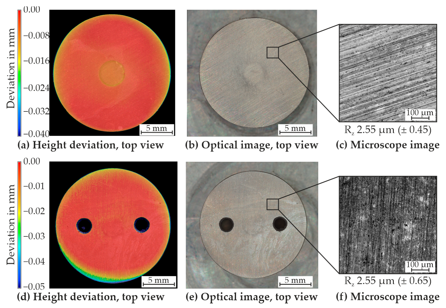
4.1. Initial State

Prior to commencing the experiments in HBSS, an analysis of the initial state was required. For this purpose, the surface of sample geometry 1 (Figure 7a–c) and 2 (Figure 7d–f) were examined with the confocal LED microscope and the 3D profilometer. In Figure 7a), the height deviation from the set base plane is visible on the 3D profilometer for sample geometry 1. It is evident that the sample does not show any major deviations from the surface baseline. Only a slight shift in the height of the sample is visible. This is important for the investigations in the HBSS with regard to the subsequent comparison of the height development after degradation. Furthermore, the overview image of the sample can be observed in Figure 7b. In this image, slight grooves caused by the manufacturing process and post-processing can be detected. These details are more clearly in the image captured using the confocal LED microscope (Figure 7c). Small inclusions are also visible in the microscope image, which could represent alloy precipitates. The surface roughness was measured, resulting in an R_z value of 2.55 µm (±0.45).

The investigation results for sample geometry 2 are depicted in Figure 7d–f. These findings align with those of sample geometry 1, as anticipated. Similar to sample geometry 1, small inclusions are identifiable in the microscope images. Moreover, a comparable R_z value of 2.55 µm (±0.65) was determined.

The results of Young’s modulus and hardness mappings from the centre of the planar sample surface (a,c; MP 2) and the centre side (b,d; MP 1) are presented in Figure 8 for sample geometry 1 as an example. When comparing the results from Young’s modulus, no difference between the two test areas could be identified (Figure 8a,b). The average Young’s modulus is about 45 GPa. In some areas, a maximum of about 80 GPa is measured. The individual higher values may be due to intermetallic compounds containing yttrium or neodymium from the alloy. Mapping from the side region shows a blue area with very low values (Figure 8b). This area represents the embedding material. A similar distribution of the maximum and minimum values within the hardness mapping of the two investigated areas is evident (Figure 8c,d). On average, a hardness of approximately 1.125 GPa was recorded. Maximum and minimum values of 3.0 GPa and 0.75 GPa, respectively, were measured.

In the etched (1% alcoholic nitric acid) metallographic images (Figure 8e,f), no difference can be seen between the edge centre and the centre side of the sample. Uneven grain sizes can be recognised in both areas. It can be assumed that the dark particles in the metallographic images are inclusions or precipitates of the alloy, which were measured as hard particles in the hardness and Young’s modulus mappings. The grain size is between a few micrometres and 25 µm in individual cases.

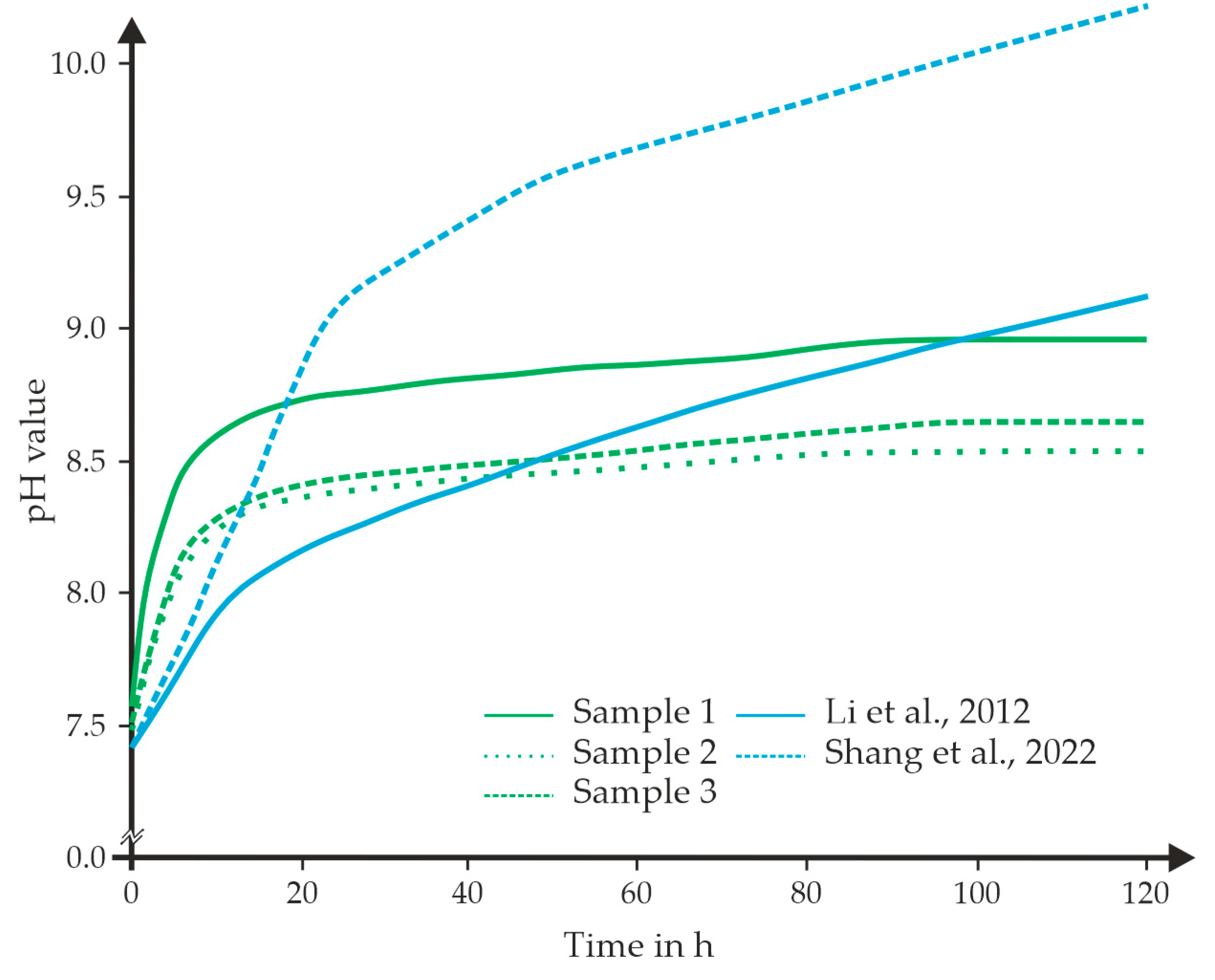
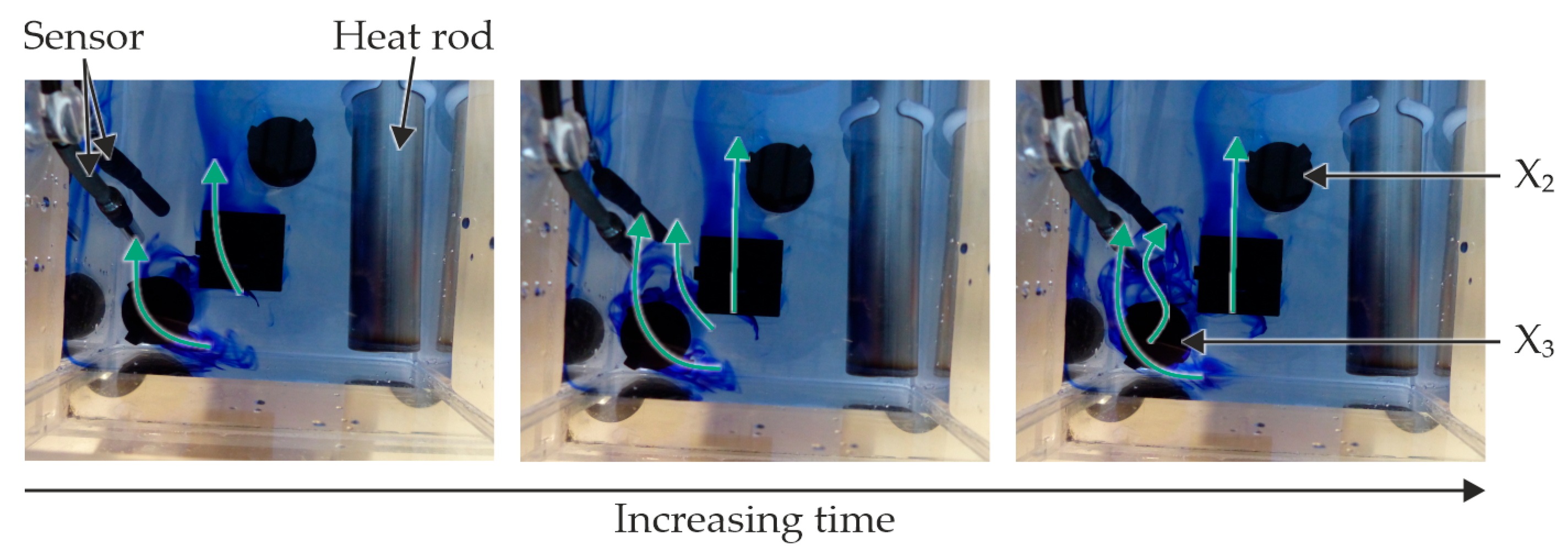
4.2. Results from the Degradation Experiments

By using HBSS as body replacement fluid without another buffer introduced, the pH value changed over the time of the experiment (Figure 9). Before starting the experiment, the pH was set to a physiological value of about 7.5. After the start of the experiment (placing the sample in the liquid), the pH value increases sharply within a short time. As a result, the value was between 8.4 and 8.8 after 20 h. In the further course, an almost constant value of 8.5 to 8.9 was reached (after 80 h). This exemplary course was observed in an approximate manner for all samples and in all experimental chambers of sample geometry 1. During all tests, the set temperature remained constant at 37 °C (±0.2).

The behaviour of the pH value in this study is improved compared to the findings of Shang et al. (V/S ratio of 40 mL/cm²) [24] and Li et al. (V/S ratio not mentioned) [27]. In both studies, WE43 samples were immersed in HBSS liquid for a defined duration, during which the pH value was observed to increase rapidly initially (pH value between 9.0 and 10.5 after 120 h). Kim et al. [25] reported a pH range of 10.0 to 10.5 after five days (V/S ratio not mentioned), whereas Bian et al. [16] measured a value of approximately 11.0 (V/S ratio of 30 mL/cm²). Comparing with the existing literature, it becomes clear that an appropriate V/S ratio must be selected. The significantly higher increase in pH value within the first five days in the studies by Shang et al. [24] and Bian et al. [16] can be explained by their lower V/S ratio. Another influence could be minimal differences in the HBSS composition. Overall, it can be stated that in the experimental chamber presented here, a pH value increase of 0.7 to 1.2 was observed within the first 24 h. This leads to the conclusion that an additional coating might be recommended for future applications to slow down degradation and, consequently, mitigate its impact on the pH value. This can reduce the body’s need to compensate for pH changes.

The results for the positioning of sample geometry 1 and 2 in the experimental chamber are shown in Figure 10. Before the start of the experiments, the roughness depth R_z was 2.55 µm for the samples (Figure 7 and Figure 10a). After five days in the HBSS, an increase in the roughness depth is measured. Depending on the positioning, the value is between 10.0 µm (X₂ sample geometry 2) and 20.5 µm (X₁ sample geometry 2). Overall, position X₁ exhibits the highest resulting roughness for both sample geometries. The spread of the values is highest for position X₁ compared to the other two positions. This greater spread can be attributed to its location in the experimental chamber. In general, both geometries lead to very similar results. An exemplary view of the surface roughness can be seen in Figure 10b. A clod-like layer structure can be observed in the topmost layer of the image. These “clods” are the degradation layer that lies loosely on top of the base material. In the bottom-most layer of the image, the base material is visible, and the initial signs of degradation can be identified.

To contextualise the results of the roughness analysis, Figure 11 presents the findings from the analysis of flow conditions. A non-directional flow is present at position X₃ (left position, largest distance to the pump). This is due to the position in the installation space, which is located directly in the corner. Position X₂ (middle position) experiences a directional flow, characterised by a constant flow that exerts uniform loads on the degradation layer due to fluid movement. Position X₁ (the smallest distance to the pump, not visible in the figure) undergoes the direct flow of the pump due to its positioning close to the pump outlet. Due to the position, more particles can detach from the degradation layer, which results in greater roughness and greater dispersion; therefore, samples from this position have been used for analyses with the Triboindenter. Based on the information from the roughness measurements and the analysis of the HBSS flow conditions, only position X₂ can be recommended for further analyses.

In addition, investigations related to hardness and Young’s modulus were carried out on sample geometry 2 (of position X₁) as an example (Figure 12). It should be noted that the degradation products were not removed before measuring. The central area (MP 2) on the sample surface of the covered part was analysed (Figure 12a,c). Additionally, the edge area (MP 1) of the borehole that had contact with HBSS was investigated (Figure 12b,d,f). In the area that had no contact with HBSS, equal values for Young’s modulus of approximately 45 GPa can be measured (Figure 12a). In the edge area, the measurements are placed in such a way that an area with localised degradation is also examined. This ensures that a possible degradation layer is also investigated, which can also be recognised in the post-image in Figure 12f. In the area at the edges where surface corrosion was present, the degradation layer was removed due to the process. Consequently, it was not possible to measure this layer. Therefore, the focus was directed towards localised degradation.

Through the analysis of Young’s modulus, it was indicated that the degradation progressed from the outside towards the inside, rather than originating internally (Figure 12b). In the area with the local degradation, lower values of around 25 GPa were determined. In some instances, these values are also slightly lower, but it is important to note the increased roughness in areas of localised degradation. This roughness might introduce minor distortions in the results; however, the overall trend remains consistent. It was to be expected that there would be a reduction in the mechanical properties in the area of degradation, as the degradation layer is described as brittle and lacking in strength. When analysing the middle sample area, a hardness of around 1.5 GPa was determined (Figure 12c). Only individual small areas with higher values of a maximum of 3 GPa and lower values of 0.75 GPa were measured. These local differences can be attributed to alloy precipitations, which were visible both in the analysis before the degradation experiments (chapter 4.1) and in the metallographic image Figure 12e. In the area of the local degradation, an average hardness of approximately 0.6 GPa was determined (Figure 12d). Occasionally, higher hardness values can be recognised around the local degradation, up to a maximum value of 4 GPa. The metallographic image in Figure 12e shows a slight change in the outer surface layer (green box). There is no uniform surface, and it appears that the outer grains have bonded together. This may indicate the presence of a degradation layer. The examination of the local degradation showed a reduction of Young’s modulus. However, this should be analysed again in further experiments to determine possible influencing factors.

In addition to the surface roughness, the influence of geometry on the mass loss can also be recognised (Figure 13a). Sample geometry 1 exhibited a higher mass loss of 0.09%, whereas sample geometry 2 experienced a mass loss of 0.06%. A similar trend can also be seen in the degradation rate (Figure 13b). Again, sample geometry 2 shows a lower degradation rate (0.25 mm/y) compared to sample geometry 1 (0.75 mm/y). The degradation rate was calculated using the linear relationship between mass loss and density (Equation (1)). Overall, it can be stated here that an influence of the sample geometry can be recognised. Although both sample geometries lose a similar mass in percentage terms, different degradation rates are calculated due to the different surface areas exposed to the medium. Both rates fall within the targeted degradation range of 0.2–0.5 mm/y, which is recommended for bone healing [20]. Consequently, both geometries could be replaced by the alloy WE43 in future applications.

For sample geometry 1, one half was covered with parafilm before the experiments (Figure 14). During the optical measurement, the influence of the degradation is made clear by a difference in the height between the covered (left half) and uncovered side (right half) (Figure 14a). Before conducting the measurements, the degradation layer was removed to prevent any distortion of the results. It can be seen that on the covered half is a smooth and even surface, which is used as a reference plane for determining the height differences. It is evident that this area was not in contact with HBSS due to the application of Parafilm, indicating that no degradation process occurred. On the uncovered half, height differences ranging from 0.02 mm to −0.05 mm are measured. On one hand, a slight uniform reduction in height is observable on the exposed side, where even degradation occurred. On the other hand, there is significant height reduction, indicative of localised degradation, in certain areas, which is highlighted by the blue regions. In some areas around the strong height reduction, there is a punctual height increase. This may indicate the accumulation of possible degradation products or measurement inaccuracies, as the height increase is very small (0.02 mm). The observed results from the optical measurement can also be seen in the top view in Figure 14b. In this instance as well, the difference between covered and uncovered areas is distinctly observable due to a variation in colour. Furthermore, both the almost uniform and the punctual/local degradation can be seen. With the help of the microscope, different areas of the sample were examined more closely (Figure 14c). Firstly, a covered area (left side) was examined in more detail. Clear scratches are visible due to the previous polishing of the sample. These observations correspond to the analyses before the start of the experiment (Figure 7). It can therefore be concluded that the Parafilm protected the part of the sample from the contact with HBSS. Moreover, areas exposed to HBSS are also analysed (right side). In Figure 14c, the scratches are less clearly visible due to the degradation of this sample area. In addition, the local degradation is visible in the lower right area of the image. Due to the depth of the degradation, it was not possible to visualise the area completely in focus.

For sample geometry 2, the left half of the specimen was also covered with parafilm before the start of the experiments (Figure 15). The optical measurement clearly shows the difference due to the influence of degradation between the covered and uncovered sides (Figure 15a). Overall, similar results are achieved here between the covered and uncovered sides compared to sample geometry 1. Increased degradation can be seen in the area of the hole. An almost uniform degradation can be recognised between the two boreholes in the uncovered area. In the far-right area, more pronounced localised grooves can be seen, which are mainly concentrated in the area of the hole. The observations from the optical measurement can also be recognised in the top view of the sample (Figure 15b). With the help of the microscope, different areas were also analysed in this sample geometry (Figure 15c). Firstly, the covered area of the sample is examined (left image). In this image, the scratches can be detected due to the pre-treatment of the sample prior to the experiments, which clearly indicates the absence of contact with HBSS. In addition, areas that had been exposed to HBSS are analysed in more detail (right image). An uneven surface is evident, with localised deeper extrema, which, as previously, cannot be fully rendered in sharp detail due to the height differences in the image.

Homogeneous degradation was observed globally across both sample geometries. However, significantly stronger, locally confined degradation in the form of pitting corrosion was also evident. This behaviour of local degradation can be explained by the phase distribution in the alloy, which was also investigated in more detail in the work by Wang et al. [18]. In their work, it was found that the α-Mg phases on the surface of the samples degrade first. In addition, individual inclusions in the alloy were observed in this work through the confocal microscope images. It is assumed that the degradation had spread along the phases and that α-Mg phases had dissolved first according to the work of Wang et al. [18].

To summarise the results, it was observed that the shortest distance (X₁) to the pump led to the greatest increase in the roughness R_z. Due to the increase in the R_z value, there was also a greater scattering of the measured values for all sample positions. Position X₁ showed the highest scatter for both sample geometries. For position X₂, only sample geometry 1 showed a greater scatter compared to sample position X₃. If the location of a possible bone implant is also taken into account, it is obvious that a purely flowing state is not suitable as an abstraction for the planned location of the application. Accordingly, the middle distance (X₂) in the experimental chamber should be targeted for further experiments. This corresponds more to a mixture of dynamic uniform flowing and static state, which corresponds to an abstraction of the state in the bone. At the same time, the influence of the sample geometry on the degradation rate should be investigated in more detail. This becomes clear from the fact that although sample geometry 2 shows the same or similar percentage loss compared to sample geometry 1, it has a lower degradation rate. The mass loss rate in mm/(cm² * day) is included in the calculation of the degradation rate. Accordingly, the lower value results from the lower initial mass and the larger surface area also plays a role.

5. Conclusions and Outlook

In this work, the experimental setup for analysing the degradation behaviour was first presented. To verify the obtained and measured values, for example, the measured pH value was compared with the data from Shang et al. [24] and Li et al. [27]. In addition, the appropriate positioning of the samples in the experimental chamber was also analysed. Three different positions were compared for this purpose. Based on the flow situation and the measured surface roughness, position X₂ is recommended for further experiments. In an abstracted form, this position best reflects the ratio of slow and uniform flow of the fluid to the subsequent implant application. Both typical forms of degradation (uniform and local degradation) could be demonstrated by optical measurement of the height differences, which were 0.02 mm for uniform degradation and up to 0.05 mm for local degradation. This once again emphasises the usability of the experimental setup. Analysis of the degradation layer revealed a reduction of mechanical properties in the degradation layer. Consequently, the degradation layer does not contribute to the additional stabilisation of a potential implant. This consideration must be taken into account when designing implants made from this material.

Overall, the results presented validate the design of the experimental chamber. Additionally, they provide an analysis of the mechanical properties of the degradation layer, facilitating the application of the WE43 alloy as an osteosynthesis implant. The next step involved conducting experiments with a constant pH value to more accurately replicate the conditions of in vivo applications. Furthermore, the influence of the choice of geometry and the manufacturing process on the application as a potential bone screw should be examined in more detail. With regard to its application as a bone screw, additional experiments should be conducted to assess a longer degradation time and to determine further mechanical properties, such as tensile strength. All these analyses can then be used as a basis for developing a numerical model to predict the degradation of magnesium alloy WE43. Thus, a realistic numerical design of implants is possible, considering the development of human bone and implant properties.

References

1. Gesundheitsberichterstattung des Bundes: Diagnosedaten der Krankenhäuser ab 2000. Available online: https://www.gbe-bund.de/gbe/pkg_isgbe5.prc_menu_olap?p_uid=gast&p_aid=57722364&p_sprache=D&p_help=0&p_indnr=550&p_indsp=&p_ityp=H&p_fid= (accessed on 25 March 2023).
2. Wintermantel, E.; Ha, S.-W. Medizintechnik: Life Science Engineering, 5th ed.; Springer: Berlin/Heidelberg, Germany, 2009. [Google Scholar]
3. Rahim, M.I.; Tavares, A.; Evertz, F.; Kieke, M.; Seitz, J.-M.; Eifler, R.; Weizbauer, A.; Willbold, E.; Jürgen Maier, H.; Glasmacher, B.; et al. Phosphate conversion coating reduces the degradation rate and suppresses side effects of metallic magnesium implants in an animal model. J. Biomed. Mater. Res. Part B Appl. Biomater. 2017, 105, 1622–1635. [Google Scholar] [CrossRef] [PubMed]
4. Grün, N.G.; Donohue, N.; Holweg, P.; Weinberg, A.-M. Resorbierbare Implantate in der Unfallchirurgie. J. Miner. Muskuloskelettale Erkrank. 2018, 25, 82–89. [Google Scholar] [CrossRef]
5. Seitz, J.-M. Entwicklung von Magnesiumlegierungen Mit Seltenen Erden Für Medizintechnische Anwendungen. Ph.D. Thesis, Leibniz University Hannover, Hannover, Germany, 2013. [Google Scholar]
6. Liu, L.; Gebresellasie, K.; Collins, B.; Zhang, H.; Xu, Z.; Sankar, J.; Lee, Y.-C.; Yun, Y. Degradation Rates of Pure Zinc, Magnesium, and Magnesium Alloys Measured by Volume Loss, Mass Loss, and Hydrogen Evolution. Appl. Sci. 2018, 8, 1459. [Google Scholar] [CrossRef]
7. Durisin, M.; Reifenrath, J.; Weber, C.M.; Eifler, R.; Maier, H.J.; Lenarz, T.; Seitz, J.-M. Biodegradable nasal stents (MgF2 -coated Mg-2 wt %Nd alloy)-A long-term in vivo study. J. Biomed. Mater. Res. Part B Appl. Biomater. 2017, 105, 350–365. [Google Scholar] [CrossRef]
8. Han, P.; Cheng, P.; Zhang, S.; Zhao, C.; Ni, J.; Zhang, Y.; Zhong, W.; Hou, P.; Zhang, X.; Zheng, Y.; et al. In vitro and in vivo studies on the degradation of high-purity Mg (99.99wt.%) screw with femoral intracondylar fractured rabbit model. Biomaterials 2015, 64, 57–69. [Google Scholar] [CrossRef]
9. Manescu, V.; Antoniac, I.; Antoniac, A.; Laptoiu, D.; Paltanea, G.; Ciocoiu, R.; Nemoianu, I.V.; Gruionu, L.G.; Dura, H. Bone Regeneration Induced by Patient-Adapted Mg Alloy-Based Scaffolds for Bone Defects: Present and Future Perspectives. Biomimetics 2023, 8, 618. [Google Scholar] [CrossRef]
10. Tan, J.; Ramakrishna, S. Applications of Magnesium and Its Alloys: A Review. Appl. Sci. 2021, 11, 6861. [Google Scholar] [CrossRef]
11. Zhao, Y.; Cui, H.; Guo, X.; Bu, C. Design and Characterization of Mg Alloy Pedicle Screws for Atlantoaxial Fixation. Metals 2023, 13, 352. [Google Scholar] [CrossRef]
12. Tsakiris, V.; Tardei, C.; Clicinschi, F.M. Biodegradable Mg alloys for orthopedic implants—A review. J. Magnes. Alloys 2021, 6, 1884–1905. [Google Scholar] [CrossRef]
13. Md Saad, A.P.; Prakoso, A.T.; Sulong, M.A.; Basri, H.; Wahjuningrum, D.A.; Syahrom, A. Impacts of dynamic degradation on the morphological and mechanical characterisation of porous magnesium scaffold. Biomech. Model. Mechanobiol. 2019, 18, 797–811. [Google Scholar] [CrossRef]
14. Staiger, M.P.; Pietak, A.M.; Huadmai, J.; Dias, G. Magnesium and its alloys as orthopedic biomaterials: A review. Biomaterials 2006, 27, 1728–1734. [Google Scholar] [CrossRef] [PubMed]
15. Seitz, J.-M.; Eifler, R.; Bach, F.-W.; Maier, H.J. Magnesium degradation products: Effects on tissue and human metabolism. J. Biomed. Mater. Res. Part A 2014, 102, 3744–3753. [Google Scholar] [CrossRef] [PubMed]
16. Bian, J.-C.; Yu, B.-Y.; Hao, J.-F.; Zhu, H.-W.; Wu, H.-S.; Chen, B.; Li, W.-R.; Li, Y.-F.; Zheng, L.; Li, R.-X. Improvement of microstructure, mechanical properties, and corrosion resistance of WE43 alloy by squeeze casting. China Foundry 2022, 19, 419–426. [Google Scholar] [CrossRef]
17. Gonzalez, J.; Hou, R.Q.; Nidadavolu, E.P.S.; Willumeit-Römer, R.; Feyerabend, F. Magnesium degradation under physiological conditions—Best practice. Bioact. Mater. 2018, 3, 174–185. [Google Scholar] [CrossRef]
18. Wang, L.; He, J.; Yu, J.; Arthanari, S.; Lee, H.; Zhang, H.; Lu, L.; Huang, G.; Xing, B.; Wang, H.; et al. A Review: Degradable Magnesium Corrosion Control for Implant Applications. Materials 2022, 15, 6197. [Google Scholar] [CrossRef]
19. Chen, Y.; Xu, Z.; Smith, C.; Sankar, J. Recent advances on the development of magnesium alloys for biodegradable implants. Acta Biomater. 2014, 10, 4561–4573. [Google Scholar] [CrossRef]
20. Shuai, C.; Li, S.; Peng, S.; Feng, P.; Lai, Y.; Gao, C. Biodegradable metallic bone implants. Mater. Chem. Front. 2019, 3, 544–562. [Google Scholar] [CrossRef]
21. Shi, Z.; Liu, M.; Atrens, A. Measurement of the corrosion rate of magnesium alloys using Tafel extrapolation. Corros. Sci. 2010, 52, 579–588. [Google Scholar] [CrossRef]
22. Radha, R.; Sreekanth, D. Insight of magnesium alloys and composites for orthopedic implant applications—A review. J. Magnes. Alloys 2017, 5, 286–312. [Google Scholar] [CrossRef]
23. Lachmayer, R.; Lippert, R.B. Additive Manufacturing Quantifiziert: Visionäre Anwendungen und Stand der Technik, 1st ed.; Springer: Berlin/Heidelberg, Germany, 2017. [Google Scholar]
24. Shang, T.; Wang, K.; Tang, S.; Shen, Y.; Zhou, L.; Zhang, L.; Zhao, Y.; Li, X.; Cai, L.; Wang, J. The Flow-Induced Degradation and Vascular Cellular Response Study of Magnesium-Based Materials. Front. Bioeng. Biotechnol. 2022, 10, 940172. [Google Scholar] [CrossRef]
25. Kim, W.-C.; Han, K.-H.; Kim, J.-G.; Yang, S.-J.; Seok, H.-K.; Han, H.-S.; Kim, Y.-Y. Effect of surface area on corrosion properties of magnesium for biomaterials. Met. Mater. Int. 2013, 19, 1131–1137. [Google Scholar] [CrossRef]
26. van Gaalen, K.; Gremse, F.; Benn, F.; McHugh, P.E.; Kopp, A.; Vaughan, T.J. Automated ex-situ detection of pitting corrosion and its effect on the mechanical integrity of rare earth magnesium alloy—WE43. Bioact. Mater. 2022, 8, 545–558. [Google Scholar] [CrossRef] [PubMed]
27. Li, N.; Guo, C.; Wu, Y.H.; Zheng, Y.F.; Ruan, L.Q. Comparative study on corrosion behaviour of pure Mg and WE43 alloy in static, stirring and flowing Hank’s solution. Corros. Eng. Sci. Technol. 2012, 47, 346–351. [Google Scholar] [CrossRef]
28. Song, G.; Atrens, A.; StJohn, D. An Hydrogen Evolution Method for the Estimation of the Corrosion Rate of Magnesium Alloys. In Magnesium Technology 2001; John Wiley & Sons, Inc.: Hoboken, NJ, USA, 2013; pp. 254–262. [Google Scholar]
29. Willumeit, R.; Feyerabend, F.; Huber, N. Magnesium degradation as determined by artificial neural networks. Acta Biomater. 2013, 9, 8722–8729. [Google Scholar] [CrossRef]
30. Klauser, H. Internal fixation of three-dimensional distal metatarsal I osteotomies in the treatment of hallux valgus deformities using biodegradable magnesium screws in comparison to titanium screws. Foot Ankle Surg. 2019, 25, 398–405. [Google Scholar] [CrossRef]
31. Zhang, R.; Zhang, Z.; Zhu, Y.; Zhao, R.; Zhang, S.; Shi, X.; Li, G.; Chen, Z.; Zhao, Y. Degradation Resistance and In Vitro Cytocompatibility of Iron-Containing Coatings Developed on WE43 Magnesium Alloy by Micro-Arc Oxidation. Coatings 2020, 10, 1138. [Google Scholar] [CrossRef]
32. Windhagen, H.; Radtke, K.; Weizbauer, A.; Diekmann, J.; Noll, Y.; Kreimeyer, U.; Schavan, R.; Stukenborg-Colsman, C.; Waizy, H. Biodegradable magnesium-based screw clinically equivalent to titanium screw in hallux valgus surgery: Short term results of the first prospective, randomized, controlled clinical pilot study. Biomed. Eng. Online 2013, 12, 62. [Google Scholar] [CrossRef]
33. Sahin, A.; Gulabi, D.; Buyukdogan, H.; Agar, A.; Kilic, B.; Mutlu, I.; Erturk, C. Is the magnesium screw as stable as the titanium screw in the fixation of first metatarsal distal chevron osteotomy? A comparative biomechanical study on sawbones models. J. Orthop. Surg. 2021, 29, 23094990211056439. [Google Scholar] [CrossRef]
34. Denkena, B.; Köhler, J.; Stieghorst, J.; Turger, A.; Seitz, J.; Fau, D.R.; Wolters, L.; Angrisani, N.; Reifenrath, J.; Helmecke, P. Influence of Stress on the Degradation Behavior of Mg LAE442 Implant Systems. Procedia CIRP 2013, 5, 189–195. [Google Scholar] [CrossRef]
35. Kirkland, N.T.; Birbilis, N.; Staiger, M.P. Assessing the corrosion of biodegradable magnesium implants: A critical review of current methodologies and their limitations. Acta Biomater. 2012, 8, 925–936. [Google Scholar] [CrossRef]
Figure 1. Schematic overview of the tensile strength via the modulus of elasticity of various materials compared to human bone (modified after [4]).
Applsci 15 03300 g001
Figure 3. CAD representation of the experimental setup.
Applsci 15 03300 g003
Figure 4. CAD model of the sample holder with and without a sample.
Applsci 15 03300 g004
Figure 5. Different positions of the samples during some tests (top view of a single experimental chamber).
Applsci 15 03300 g005
Figure 6. The two different geometry samples both Ø 18 mm, height 10 mm; (a,b) to analyse the influence on the degradation rate and the information on the V/S ratio of the two sample geometries (HBSS volume of 1500 cm3) (c).
Applsci 15 03300 g006
Figure 7. Exemplary result of the optical measurement from the initial state of sample geometry 1 (ac) and sample geometry 2 (df).
Applsci 15 03300 g007
Figure 8. Exemplary comparison of Young’s modulus and hardness measurements at two positions (centre of the surface (a,c) MP 2 and centre side of the sample (b,d) MP 1), etched metallographic images (e,f) of the sample geometry 1.
Applsci 15 03300 g008
Figure 9. Development of the pH value during the experiment time of sample geometry 1 and the comparison with literature values [24,27].
Applsci 15 03300 g009
Figure 10. Roughness development (a) of all positions; an image of the roughness (b) of geometry 2 of sample position X1.
Applsci 15 03300 g010
Figure 11. Images of the flow behaviour of the HBSS in one experimental chamber (back section), with the colour added to clarify the flow, without a sample present in the chamber.
Applsci 15 03300 g011
Figure 12. Investigations with the Triboindenter after five days in the body replacement fluid of sample geometry 2 ((a,c) a region without contact to the fluid; (b,d) with contact to the fluid; (f) postscan of the investigations (b,d)) and (e) metallographic image of the centre side with contact to the fluid.
Applsci 15 03300 g012
Figure 13. Mass development (a) as well as the degradation rate (b) of position X2 for sample geometry 1 and 2.
Applsci 15 03300 g013
Figure 14. Optical analysis results of sample geometry 1 after five days in the HBSS by (a) optical measurement (b) overview image and (c) microscope images.
Applsci 15 03300 g014
Figure 15. Optical analysis results of sample geometry 2 after five days in the HBSS ((a,b) optical measurement; (c) microscope images).
Applsci 15 03300 g015