Application of Modeling and Simulation in a Self-Reprogrammable Prototype of a Manufacturing System

Abstract

Shorter product life cycles and the growing demand for mass customization have led to the development of complex production systems, which are crucial for maintaining competitiveness. In this context, digital technologies and simulation tools play a fundamental role in integrating virtual and physical systems to enhance operational performance. This study presents a prototype for self-programming manufacturing systems, achieved through the integration of computer simulation and production management tools, leveraging the Digital Twin (DT) concept. To validate this approach, a prototype capable of interacting with a simulation model was developed. In the event of a failure that compromises product delivery conditions, the simulation model is activated to reprogram the production system’s operating parameters, ensuring compliance with initial production requirements and minimizing the impact of disruptions. The tests confirmed effective data exchange between the physical and virtual environments. Additionally, intentional failures were introduced in the real environment to assess system behavior. Each time a failure occurred, the simulation model generated new operating parameters, adjusting the working speed in the real environment and thereby maintaining the production system’s ability to meet its requirements. Consolidating the application of self-reprogramming.

1. Introduction

Production systems have undergone significant growth since the Industrial Revolution in the late 18th century. This expansion has been primarily driven by advancements in technologies such as machinery, energy systems, and computing. Moreover, in recent decades, the digital revolution and globalization have introduced profound transformations in consumer markets, consequently reshaping production systems [1].

As a result, numerous companies have expanded their operations internationally, intensifying market competition. This increased competitiveness has led to a significant diversification of product offerings, posing challenges in production management due to shorter product life cycles and a growing demand for personalization and mass customization [2,3]. Several authors assert that the complexity of production systems is expected to increase due to escalating customer demands, necessitating the implementation of more flexible and agile manufacturing systems [4]. In this scenario, the most impacted areas include production scheduling and the management of operational failures in manufacturing systems, such as rework and supply chain disruptions [5,6,7,8].

To address these challenges, various technologies and computational tools have been developed. Among them, digitalization stands out as a transformative innovation, enabling the consolidation of business data into virtual databases. Another significant advancement involves the application of production simulation software, which facilitates the creation of digital models to evaluate and optimize manufacturing processes within a virtual environment, thereby minimizing disruptions in real-world operations [9,10,11].

However, for simulation models to effectively support decision-making, it is crucial to ensure high-quality modeling, which, in turn, depends on the ability to collect and process data from the production system. The evolution of sensors and electronic components used in manufacturing has significantly enhanced data collection and processing capabilities [12]. The integration of these data with simulation models, in conjunction with optimization tools, enables more effective decision-making for manufacturing management [6,13]. In this context, the concept of smart factories has emerged [12,14,15].

In recent years, simulation models have evolved into Digital Twins (DT), wherein the digital environment maintains continuous connectivity with the physical environment through sensors that collect real-time data and transmit it to the models. This connectivity significantly enhances the accuracy of analyses compared to traditional production modeling methods [16,17,18]. This real-time data exchange mechanism has become feasible due to advancements in Internet of Things (IoT) tools and concepts [19]. Consequently, DT-based decision-making has become faster and more precise, owing to the integration of production simulation with optimization algorithms, supported by mathematical models and Artificial Intelligence (AI) tools, aligning with the requirements of Industry 4.0 [6,8,20,21,22].

Cañas et al. (2021) argue that Industry 4.0 enables the real-time collection and synchronization of data, allowing manufacturing systems to dynamically adjust to product variations or process failures [12]. However, the architecture of Industry 4.0 still requires further development to facilitate the efficient simulation of complex environments. This involves several critical steps, including real-time data acquisition, integration of these data into DT-based simulation models, optimization processes, and automated reprogramming of production systems [23]. A notable gap exists between the output of DT systems and the input requirements of production systems, which is conceptually linked to the goal of achieving self-reprogramming capabilities—one of the fundamental pillars of Industry 4.0 [2,24].

The successful implementation of DT concepts relies on a well-structured simulation model and a high level of connectivity between physical and virtual environments. This integration allows the real-world system to benefit from insights generated by simulation models, thereby enhancing decision-making in production scheduling [21,25]. In this regard, Rafael et al. (2020) highlight that the adoption of Industry 4.0 necessitates the digitalization of the entire manufacturing system, leading to improvements in productivity, efficiency, flexibility, and agility—key factors for enabling mass customization, which is essential for modern factories [6,15].

The use of digital models, in conjunction with optimization tools, offers significant benefits for supporting decision-making in manufacturing. One notable advantage is observed in production scheduling when simulation models incorporate Genetic Algorithm techniques [26,27]. Despite the benefits of using simulation and Digital Twins (DT) to aid decision-making in manufacturing, the widespread application of DT remains challenging due to the complexities of real-time data exchange and its implementation as an autonomous optimization tool [28].

This paper proposes a technical architecture for developing a simulation engine capable of real-time data exchange between a manufacturing system and its digital counterpart. The primary objective is to create an integrated environment that seamlessly connects physical and virtual domains, enabling automatic fault detection, optimization, and corrective actions without human intervention. This study focuses on developing a prototype that integrates simulation, production management, data collection, and optimization tools, leveraging the principles of DT.

This research contributes to bridging the gap between theoretical advancements and practical applications of DT. Furthermore, it explores the concepts of self-reprogramming and autonomy, particularly emphasizing a DT’s ability to dynamically adapt its model in real time and respond to changes in the physical environment [16].

The remainder of this paper is structured as follows: Section 2 explores the concept of DT in detail. Section 3 describes the research methodology, including the classification and stages of the investigation. Section 4 presents the prototype design, encompassing the management system perspective, prototype layers, logical programming model, and physical resources. Section 5 discusses the results of the simulation tests and evaluates the physical performance of the system. Finally, Section 6 concludes the study by summarizing key findings and providing insights for future research.

2. Digital Twin

The DT can be defined as a virtual representation of products, processes, or services, enabling the replication of real-world characteristics in a simulated environment [16]. DT facilitates the modeling of real systems in a digital architecture, allowing interaction and data exchange among interconnected systems [29]. This interaction is typically established through real-time data exchange enabled by sensors [30,31].

Digital models used for DT can be expressed in four dimensions: the Geometric Model, which represents geometry and physical connections; the Physical Model, which encompasses its properties and characteristics; the Behavioral Model, which represents its dynamism in response to external actions; and the Rule Model, which can explore tacit concepts, serving as a basis for building more intelligent models [32].

In essence, a DT is characterized by three fundamental elements: a physical component, a virtual representation, and the connection between them. This concept emerged in 2002 at the University of Michigan by Singh et.al. [33].

Some researchers classify DT components into two categories: Elementary Components, these include the physical component, the virtual representation, and the connection linking the physical and virtual environments; Imperative Components, these encompass IoT devices, collected and stored data, machine learning models for prediction, response, and optimization, data and information flow security, and the performance evaluation of the virtual representation [16,22].

The DT concept differentiates itself from Digital Models, Virtual Factory Models, and Product Lifecycle Management (PLM) systems through some key features: Data Flow Integration, seamless integration of data between the physical system and the digital model; Real-Time Synchronization, continuous synchronization of virtual factory models with real-time data; Component Information Management, comprehensive capture and management of information from product components; Smart Products Integration, interfacing with other advanced technologies; Model Clustering, enabling real-time data monitoring and processing [8,16]. Additionally, the DT environment incorporates continuous learning and self-updating capabilities based on data collected through sensors or other external sources [30].

There are essentially three levels of integration between the real and digital environments: Digital Model, characterized by the manual exchange of data between the real and virtual environments; Digital Shadow, where data flows automatically from the real system to the virtual environment, but the exchange of data from the virtual system to the real one is performed manually; and DT, where data flows automatically in both directions between the virtual and real environments [33].

DT allows the convergence of simulation, prototyping, real-time monitoring, analytics structuring, and optimization technologies. However, implementing DT is intrinsically tied to other technologies, such as integrated devices, big data, and machine learning tools. These dependencies affect the understanding and application of DT models, as successful implementation requires a high level of technological maturity and seamless integration of complementary technologies [16]. DT relies on robust simulation models that rely on data received in real time, which in turn benefits from the results offered by the simulation [34].

Despite these challenges, DT presents several benefits, including: the capability to conduct complex testing without affecting the real environment; cost reduction by minimizing the need for physical prototypes; shortened project timelines; development of machine learning models to support decision-making processes. Through these capabilities, DT enables the representation of design, testing, production, and operational processes within a virtual environment [30]. However, the adoption of DT poses significant challenges for small and medium-sized enterprises (SMEs), primarily due to high investment costs and the need for skilled teams in Engineering and Information Technology (IT) [29].

Among the challenges for implementation, the following stand out: security; the complexity in the implementation is proportional to the complexity of the real system operation; interoperability among different systems; data mining and control; cost of implementing some technologies without bringing clear value to the business; dependence on other technologies for operationalization; managing large amounts of data from different sources [30,35].

The application of DT largely depends on a company’s strategic objectives. These applications may be tailored to specific products or processes or implemented across entire product lines and manufacturing systems. Some researchers argue that DT offers a new perspective on simulation by advancing digitalization and enabling real-time data access [16,36].

This advancement can be supported by data collection systems such as Programmable Logic Controllers (PLCs), Manufacturing Execution Systems (MES), and Enterprise Resource Planning (ERP) platforms, which can be integrated with simulation and optimization tools, such as Advanced Process Control (APC). Additionally, technologies like Augmented Reality (AR) can enhance simulation environments by facilitating human interaction in manufacturing operations, such as assembly tasks [35].

In general, research on DT technology has grown considerably in recent years. Approximately 47.89% of publications are related to the manufacturing sector, 12.32% pertain to the energy sector, and 7.39% focus on aerospace applications. Mechanical Engineering accounts for slightly more than 50% of studies related to DT [32].

The application of DT in human-robot collaboration (Human-Robot Collaboration—HRC) and learning systems has become essential in modern manufacturing, enabling tasks to be executed with greater efficiency and flexibility. In this context, DT serves as a powerful tool, providing high-fidelity virtual representations of physical systems, which facilitate real-time monitoring, simulation, and collaborative processes optimization [37].

Despite their transformative potential, the widespread adoption of DTs faces several critical challenges: Absence of Universal Standards: The absence of a standardized reference framework hinders interoperability and integration across different DT systems and applications; Dependence on Emerging Technologies: DTs heavily rely on rapidly evolving technologies such as IoT, big data, and machine learning, making system compatibility and updates a persistent challenge; Security and Privacy Concerns: The extensive collection and exchange of sensitive data raise concerns regarding unauthorized access and potential privacy breaches; Absence of Performance Metrics: The absence of well-defined evaluation criteria impedes the accurate assessment of DT effectiveness and limits the comparability of different implementations [16].

Furthermore, the implementation of DT presents additional challenges: Data Integration: The accurate and real-time acquisition and consolidation of data are fundamental to the effectiveness of DT; Systems Interoperability: Ensuring seamless interaction between DT and diverse platforms and devices is critical for successful deployment; Data Security and Privacy: Safeguarding the sensitive information processed by DT is essential to maintaining trust among stakeholders [38].

3. Research Methodology

This work constitutes applied research, focusing on the development of a manufacturing system prototype that integrates modeling and simulation to explore the practical application of the DT concept in production process representation. Additionally, the study adopts an exploratory approach, presenting an in-depth examination of DT architecture, simulation perspectives, and its application in manufacturing processes. This foundation is built on a review of the literature, aimed at establishing meaningful connections within this domain.

The research included a case study conducted at the laboratory of the School of Mechanical Engineering at Unicamp’s main campus. The laboratory provided essential support for this investigation, offering physical resources and access to its technical team to assist in developing the prototype used to test the DT concept.

This study was organized into several stages, ranging from the theoretical phase to the structuring of the case study, which included the development and testing of the prototype according to the steps below:

• Step 1: This phase involved defining DT concepts, understanding simulation applications, and positioning DT within the context of process simulation;
• Step 2: Selection of the simulation tool for the project. The simulation software Plant Simulation^® version 16 by SIEMENS was used in this stage. Additionally, the programming language SimTalk was employed, as it is the standard language used within this software environment;
• Step 3: This stage focuses on comprehending the simulation environment and designing a real-time data exchange model between the manufacturing system and the simulation model;
• Stage 4: A simulation model was created, along with a mechanism capable of detecting failures in the production system and initiating optimization routines without human intervention;
• Step 5: Development of both the physical and virtual prototypes of the manufacturing system and establishment of the connection between them. Key activities included automating system operations and structuring computer simulations with self-reprogramming capabilities;
• Step 6: The final stage involved operating the prototype, monitoring information flows between the physical and virtual environments, and validating the execution of the reprogramming model.

This work was developed based on the simplification of a production system. However, since it is a prototype, a simple operating mechanism was chosen, controlling only the time, number of parts and speed variables. Additionally, the speed variable is adjusted to regulate the system’s work rhythm. Therefore, this study is limited to modifying a single operating variable.

4. Project Architecture

Manufacturing systems based on Industry 4.0 concepts must be able to receive information from the sensors and mechanisms. These sensors identify actions such as processing time, failures, setups, and equipment availability, in real time. The collected data are used as input for digital tools, such as Discrete Event Simulation and DT, supporting decision making.

Autonomous decision-making based on simulation requires that the simulation model and the production system be connected by software and devices responsible for managing production data. Figure 1 shows these connections.

Figure 1 shows the tools used in the integration between the real and virtual systems. Each of them has specific functions, and they are discussed below:

• Management System: It provides production sequencing. In addition, it defines manufacturing priorities for both the physical and the simulation model;
• Production system: It is a set of resources available for manufacturing products, such as workers and equipment;
• Operational data collection software: This group has Software MES (Syneco V. 2.5.15), Radio Frequency Identification (RFID), sensors, and other devices used to collect operational data from the production system, such as: operating time, failures, equipment availability, human resources availability, among others. This set of software and sensors is responsible for providing real-time data to the simulation model to keep it updated, and works in parallel with the production system;
• Virtual system: The virtual system is based on a simulation model operating in parallel with the real manufacturing system, embodying the concept of a DT. However, to enable production rescheduling after diagnosing a failure, the simulation model must meet the following requirements:
• Data input block: The simulation model requires input of management and operational data that directly influences its performance. This data is provided through the data input block, which maintains a constant connection with the data collection system. For example, if the operating time of a workstation differs from the parameters currently set in the simulation model, this updated operating time must be incorporated into the model to maintain accuracy;
• Trigger: The trigger represents a programming logic designed to detect failures in the production system and initiate the optimization process. For instance, consider a production system comprising four machines, designed to produce a specific family of products, and operating under a predefined production sequence. If one of the machines experiences a failure and becomes unavailable for a certain period, the production sequence must be recalculated. Simultaneously, information about the machine’s unavailability is sent to the simulation model, which receives a command to determine an optimal sequencing strategy based on the updated manufacturing conditions;
• Optimization: Following the failure signal generated by the trigger, the simulation model initiates the optimization process based on pre-established programming logic. For example, optimization could involve creating a revised production sequencing using Genetic Algorithms. This approach enables the system to account for real-time constraints and propose the most efficient course of action;
• Results: Once the optimization tool identifies the necessary corrective actions, the corresponding data is transmitted to the production management system. This ensures that the manufacturing system activities are updated to reflect the new plan. For example, a revised production sequence could be implemented to minimize production losses caused by the failure.

4.1. Architecture of the Real Environment

The real environment refers to the physical space where manufacturing tasks occur, encompassing both material transformation and movement activities required for product manufacturing. In this project, a part-handling system was employed as a practical model to study and validate the proposed concepts. A set of sensors and electronic devices was installed to monitor the actions of this movement system. Additionally, these electronic devices can receive information from the DT model and autonomously reprogram the real environment.

Initially, the interactions among the various systems utilized in the project were defined, as illustrated in Figure 2. The proposed architecture comprises four distinct layers, categorized based on the functions of the components employed in the project:

• Layer 0 (User layer): It represents the human component of the system. In this layer the user will be able to control the system, visualize the data and analyze the results;
• Layer 1 (Software layer): It is the connection between the user and the control layer, responsible for showing the system functionalities to the user. It is composed of the following programs: (a) Plant Simulation, (b) KASSL OPC Client, (c) Syneco, each one responsible for an operating sector;
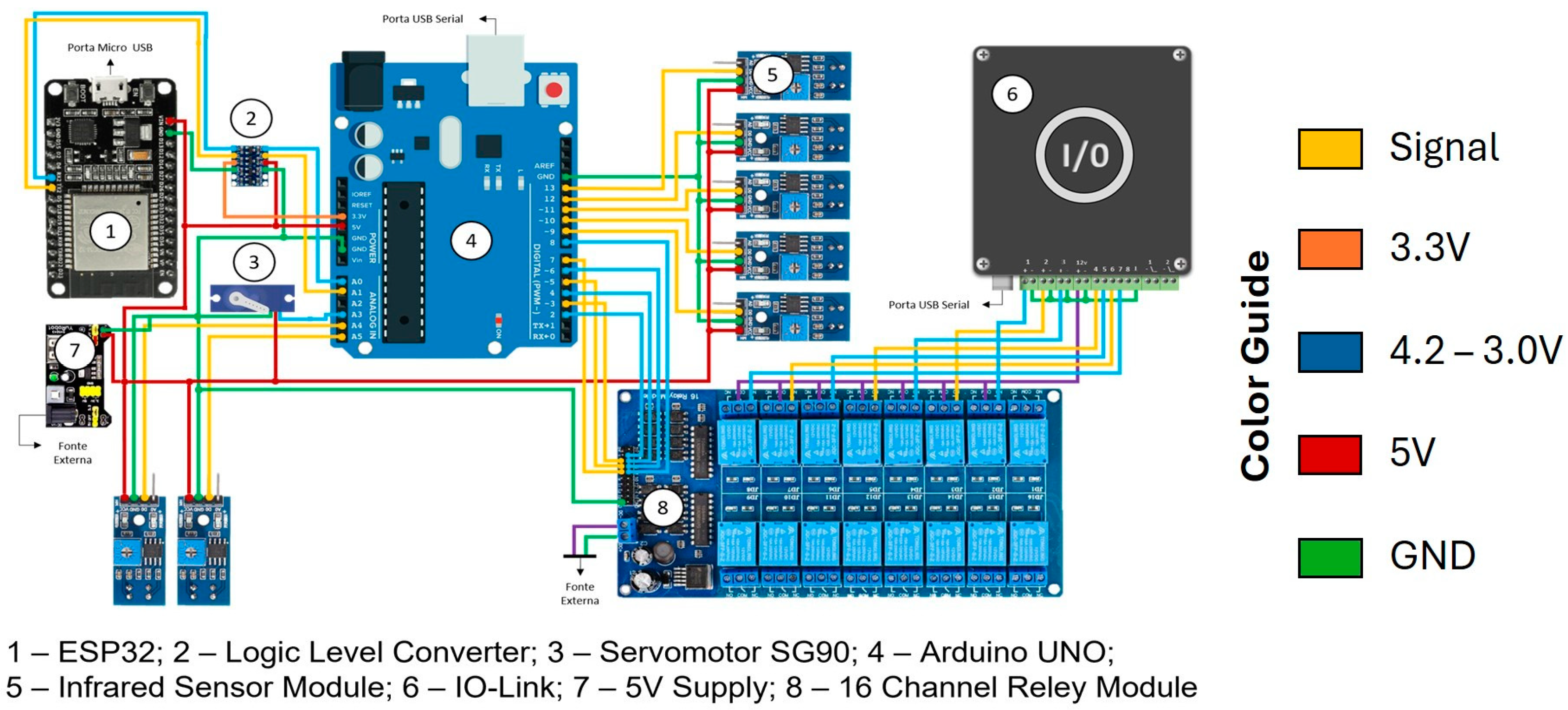
• Layer 2 (Control layer): This layer manages the system and was mostly developed by Arduino Uno and is intended to control system operations. However, there are other devices related to control, such as: Computer, responsible for the integration between the Arduino UNO R3 software and hardware; A pair of ESP32, responsible for wireless communication between the transport and the system; IO communication module, which sends data to Syneco V. 2.5.15. This layer has several communication protocols, in addition to an important integration among all components, hardware devices and software;
• Layer 3 (Devices layer): It manages the interaction between the system and the physical environment, containing the sensors responsible for collecting the required information for the system operation. In addition, there are actuators that generate the system’s response to external actions.

The Arduino was used for its versatility and large amount of documentation available online, while the ESP32 was used because it allows integration via Bluetooth, WiFi and ESP-Now. In addition, the low cost and availability of the components contributed positively to the choice. Systems with greater distances and greater amounts of data being exchanged require more robust components. However, the prototype has a maximum distance of 1.2 m between components, thus making the Arduino and ESP32 sufficient.

The data generated by the software shown in Figure 3 is connected to the Arduino platform, which was developed based on OPC-DA variables. On this platform, the collected data are treated in such a way that the software can use them in transport optimization.

In Layer 3, the variables traveled time and number of transported parts are collected, where the first variable is converted from time to speed.

Layer 2 manages the data collected from the system and is divided into two groups: static data, which has fixed results; dynamic data, which is constantly updated and depends on variables collected by the hardware.

Static values consist of: Organization, defines the quantity of order and the sections that the transport must cover; Dimensions, defines the distance that will be covered in each section; and Sensing, calibrates the sensors to detect the presence of transport at the workstation, in addition to counting the number of parts that were transported.

The dynamic data: Time, calculates the transport time interval based on the transport position; Speed is calculated based on the time taken to travel the defined distance; and Translation, which transforms the variables obtained into variables that will be transmitted to simulation software.

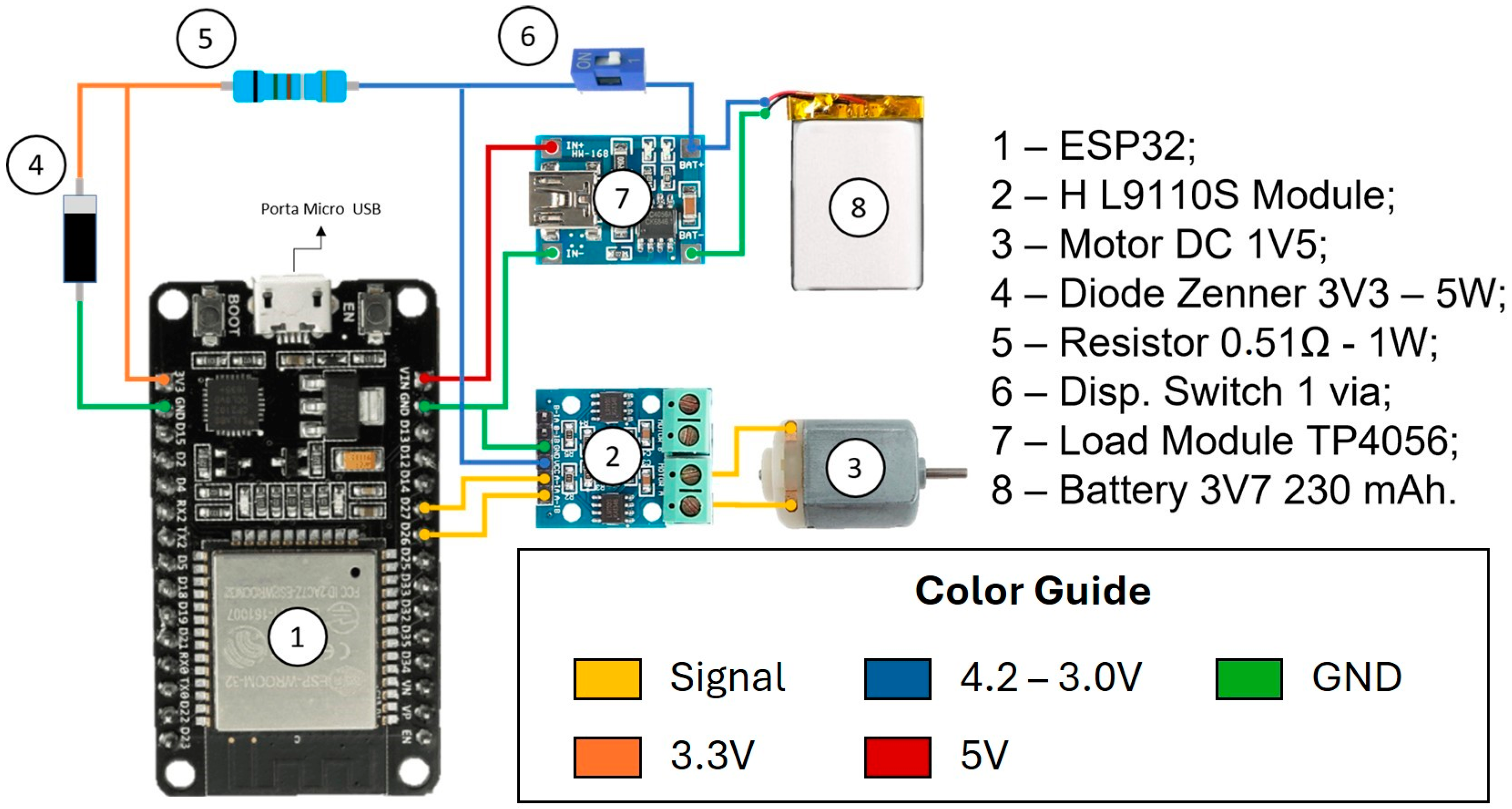
Finally, the real environment was developed to collect, analyze, and share the data generated. The track controls the general data of the system, collecting data from the sensors, sending it to Plant Simulation and returning the speed to the transport vehicle, Figure 3. The Arduino uno is responsible for monitoring the position of the vehicle and the number of charges deposited. The transporter was designed to maintain contact between the track and the Arduino controller in real time. Furthermore, the engine can change the speed to work at the best speed, defined by the virtual system, Figure 4.

4.2. Virtual Environment

Initially, the development of the simulation model followed the steps of traditional modeling, where data collection and a thorough understanding of the system’s practical functioning are fundamental to the initial stages of the project.

The data collected were: Operating time for each part of the process; Transport speed at all points; Distance traveled; Number of parts transported in each cycle; Faults; and Actual system operating behavior.

However, this specific model incorporates unique characteristics, with real-time data exchange being among the most significant. Consequently, it was essential to prepare the simulation model to receive data from sensors installed in the real environment. For instance, transport speed parameters were treated as variables depending on the status of production plan fulfillment, as determined by the following equation.

$$Vt={\displaystyle \frac{\frac{Qi - Qe}{4}\ast Pp}{Tdi-Tg}}\ast FC$$

(1)

• Vt = Transport speed;
• Qi = Parts initially planned;
• Qe = Parts delivered;
• Pp = Perimeter;
• Tdi = Initial available time;
• Tg = Time spent.

This equation allows the transport speed to be adjusted according to the current condition of the process. The ideal transport speed that fulfills the delivery deadline, and it is based on the variable quantity of parts to be transported (Qi—Qe) and available working time (Tdi—Tg). These two variables are input into the simulation model through communication between the simulation and the real environment.

Therefore, when the system identifies a delay in fulfilling the order, the transport speed is recalculated so that all parts are delivered on time.

4.2.1. Communication Between Real and Virtual Environments

To enable real-time communication, sensors installed in the physical system capture data, which is then transmitted to the simulation model. In this study, the variables identified for real-time monitoring were Cycle Time and Number of Parts Transported. These variables are sent to and processed within the Arduino database. Consequently, all parameters required for input into the simulation model are managed through defined gateways and linked to the simulation model.

In the Plant Simulation V.16 software, the tool responsible for identifying and reading data from the gateways is OPC (Open Platform Communications). OPC establishes communication between controllers and automation systems to facilitate real-time data exchange, allowing the simulation model to utilize the production system’s operating parameters. Additionally, OPC enables data transmission from the virtual environment back to the manufacturing system. 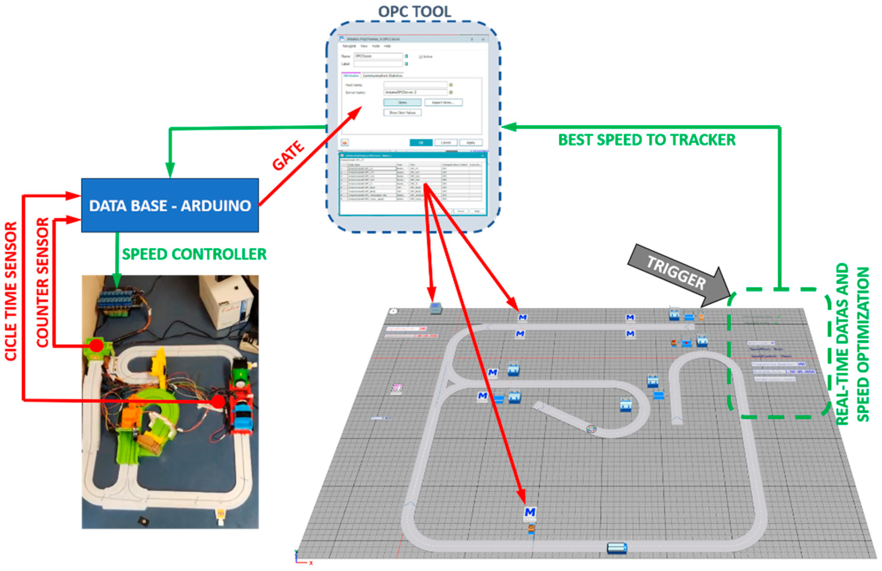Figure 5 illustrates the application of the OPC tool in facilitating communication between the simulation model and the real system.

Data is acquired from the real environment through sensors and transmitted to the Arduino database, which maintains continuous communication with the simulation model’s OPC tool via a port called Gate. At each work cycle, the simulation model computes the optimal operating speed of the conveyor and transmits the corresponding value to the OPC. Through the same Gate port, this information is relayed to the Arduino and subsequently transmitted to the conveyor via the ESP32 board, thereby adjusting the conveyor motor speed accordingly.

4.2.2. Trigger Logic

The requirement for this project is that the manufacturing system must transport a specific number of parts within a defined timeframe. The conveyor operates in a fixed and cyclical path, with each transport cycle carrying four parts. Based on this information, the transport speed and the number of cycles is determined to meet the production plan.

Given that the system operates in a closed circuit, two control points were implemented. The first control point is located at the unloading station, where the transported parts are counted, and the remaining time to complete all deliveries is tracked. At the end of each cycle, real-time data is transmitted to the simulation model. In the event of a failure, this information is forwarded to the optimization block, where the optimal speed to correct or minimize the issue is calculated. A signal is then transmitted to adjust the working speed accordingly.

The second control point is positioned at the starting point, where speed adjustments are applied. Speed reprogramming is carried out using a signal emitted by the simulation model through the same data input port. Since the conveyor is designed to respond to this signal by adjusting its operational speed, the system continuously operates at the optimal speed required to fulfill the production plan.

5. Test and Results

The model validation was carried out considering a 95% confidence interval. All data related to cycle time virtual and real are shown in

Table 1. Validation model.

	Real Time (s) Speed 11 cm/s	Virtual Time (s) Speed 11 cm/s	Real Time (s) Speed 15 cm/s	Virtual Time (s) Speed 15 cm/s
Cycle 1	61.20	62.80	45.10	46.10
Cycle 2	61.60	61.20	45.80	45.80
Cycle 3	61.00	61.10	46.30	46.60
Cycle 4	64.30	62.00	48.80	44.80
Cycle 5	62.70	63.10	46.90	45.60
Cycle 6	61.90	61.20	47.20	44.90
Cycle 7	63.40	62.10	45.90	46.10
Cycle 8	62.60	62.90	47.10	45.70
Cycle 9	63.10	63.10	46.30	44.80
Cycle 10	63.70	64.20	47.40	47.90
Mean	62.55	62.37	46.68	45.83
Standard Deviation	1.05	0.97	0.98	0.90
Validation—95% confidence interval	0.828		0.031
	−1.188		−1.731

.

Using the validation Equation (2) through the confidence interval, it is possible to state that the developed simulation model adheres to the real system by 95%.

$$\overline{Xs}+\overline{Xr}\pm t_{1n-1,{\displaystyle \frac{\propto }{2}}}\sqrt{{\displaystyle \frac{{Ss}^2+{Sr}^2}{n}}}$$

(2)

• Xs = Simulation Mean
• Xr = Real Mean
• Ss = Simulation Standard Deviation
• Sr = Real Standard Deviation
• α = 0.05
• t = 2.23 (according to table t of Student)

The development of the simulation model followed the recommendations in the previous section. For this, three programming codes were developed, and they can receive data from the real system and apply the work speed optimization equation.

Figure 6 illustrates the development of the simulation model for this project, in which the codes “MethodCycles” and “MethodTimes” process variables received from the real system via the OPC tool. This data is utilized to calculate the number of cycles the system must execute and the time available to complete the part deliveries. These values are then applied to the equation developed in “MethodSpeedControl,” which determines the optimal operating speed for the real system.

Code A: Method Speed Control. This method consists of multiplying the number of remaining cycles by the perimeter (670cm) and dividing by the remaining time, thus determining the ideal working speed.

            SpeedControl:= speed;

                         Is

                         Do

            SpeedControl: MethodCycles ∗ 670/MethodTime;

                         End;

Code B: Method Cycles. This method consists of subtracting the number of scheduled parts from the number of parts already transported and dividing by the number of parts per cycle, thus determining the number of remaining cycles.

            Cycles:= integer;

                         Is

                         Do

            Cycles:= Programmed_Quantity − Drain.StatNumOut/4;

                         End;

Code C: Methode Time. This method consists of subtracting the planned work time from the time spent, thus determining the remaining time.

            Times:= time;

                         Is

                         Do

            Times:= TimeToDo − EventController.SimTime;

                         End;

To validate the operation of this prototype, three tests were conducted, each defined by the following initial requirements:

• Test 1—Transport 40 parts within 550 s.
• Test 2—Transport 40 parts within 600 s.
• Test 3—Transport 24 parts within 300 s.

The initial transport cycle durations are set at 55 s, 60 s, and 50 s, respectively. Correspondingly, the initial conveyor speeds are 11 cm/s, 10.5 cm/s, and 13 cm/s.

A physical constraint limits the system to transporting a maximum of four parts per cycle; however, instances where fewer than four parts are moved may occur. Additionally, variations in cycle duration can arise due to stochastic failures occurring at specific part-handling stations. Both scenarios are classified as failures.

Table 2. Test 1—data.

TEST 1—DATA
Cycles	Total Parts (Units)	Increment (Units)	Cycle Time (s)	Total Time (s)	Available Time (s)	Speed (cm/s)
Cycle 0	0	0	0	0.0	550.0	0
Cycle 1	4	4	59.4	59.4	490.6	11
Cycle 2	8	4	58.1	117.5	432.5	11.5
Cycle 3	10	2	57.8	175.3	374.7	11.5
Cycle 4	14	4	54.0	229.3	320.7	12.5
Cycle 5	16	2	48.9	278.2	271.8	12.7
Cycle 6	20	4	45.5	323.7	226.3	13.8
Cycle 7	24	4	45.6	369.3	180.7	13.8
Cycle 8	28	4	56.1	425.4	124.6	13.9
Cycle 9	32	4	41.6	467.0	83.0	15.8
Cycle 10	36	4	41.1	508.1	41.9	15.7
Cycle 11	40	4	41.3	549.4	0.6	15.7

,

Table 3. Test 2—data.

TEST 2—DATA
Cycles	Total Parts (Units)	Increment (Units)	Cycle Time (s)	Total Time (s)	Available Time (s)	Speed (cm/s)
Cycle 0	0	0	0	0	600	0
Cycle 1	4	4	62.20	62.2	537.80	10.5
Cycle 2	4	0	59.9	122.1	477.90	10.5
Cycle 3	8	4	54.4	176.5	423.50	12.3
Cycle 4	12	4	54.7	231.2	368.80	12.3
Cycle 5	16	4	56.1	287.3	312.70	12.4
Cycle 6	20	4	69.7	357	243.00	12.5
Cycle 7	24	4	49.2	406.2	193.80	15.8
Cycle 8	28	4	48.8	455	145.00	15.6
Cycle 9	32	4	48.5	503.5	96.50	15.6
Cycle 10	36	4	48.1	551.6	48.40	15.7
Cycle 11	40	4	49.3	600.9	−0.90	15.9

and

Table 4. Test 3—data.

TEST 3—DATA
Cycles	Total Parts (Units)	Increment (Units)	Cycle Time (s)	Total Time (s)	Available Time (s)	Speed (cm/s)
Cycle 0	0	0	0	0	300	0
Cycle 1	4	4	52.8	52.8	247.20	13
Cycle 2	8	4	52.5	105.3	194.70	13.1
Cycle 3	12	4	64.1	169.4	130.60	13.4
Cycle 4	16	4	44.1	213.5	86.50	16.2
Cycle 5	20	4	43.8	257.3	42.70	15.7
Cycle 6	24	4	43.8	301.1	−1.10	16.1

present the data collected during Tests 1, 2, and 3, respectively. The “Total Parts” columns indicate the cumulative number of parts transported per cycle, as well as the individual count of parts moved in each cycle. These values are incorporated into the simulation model based on data retrieved from count sensors. The “Cycle Time” columns display the recorded cycle durations, obtained from position sensors installed along the conveyor track. These measures facilitate the calculation of total operational time and the remaining time available to fulfill production requirements.

Using this dataset, the equation described earlier is applied to determine the optimal conveyor speed necessary to meet the specified production targets. The computed speed values are presented in the final column, named “Speed”.

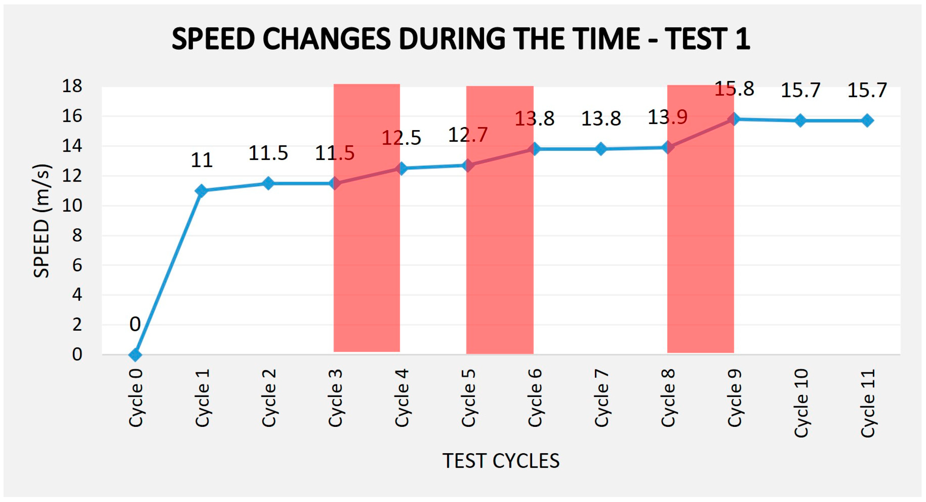
The data presented in Table 2 indicate that conveyor speed adjustments were required at three specific points during the process, occurring in cycles 3, 5, and 8. In the first two instances, these adjustments were necessitated by failures in the loading process, which resulted in the conveyor system transporting only two parts per cycle. In cycle 8, a failure at the intermediate workstation caused a 12 s delay in the cycle.

In each of these cases, the simulation model processed the real-time data, activated the control trigger, and computed the optimal speed adjustment to mitigate the issue. The conveyor, operating autonomously, implemented the new speed parameters to adhere to the predefined production time of 550 s. As a result of these corrective measures, the total duration required to transport all 40 parts was 549.4 s. Due to loading failures in cycles 3 and 5, the process required 11 work cycles instead of the initially planned 10.

Figure 7 illustrates the changes in conveyor speed across work cycles. The data clearly demonstrates that upon detecting a failure, the system dynamically adjusts the speed to compensate for lost time and maintain production efficiency.

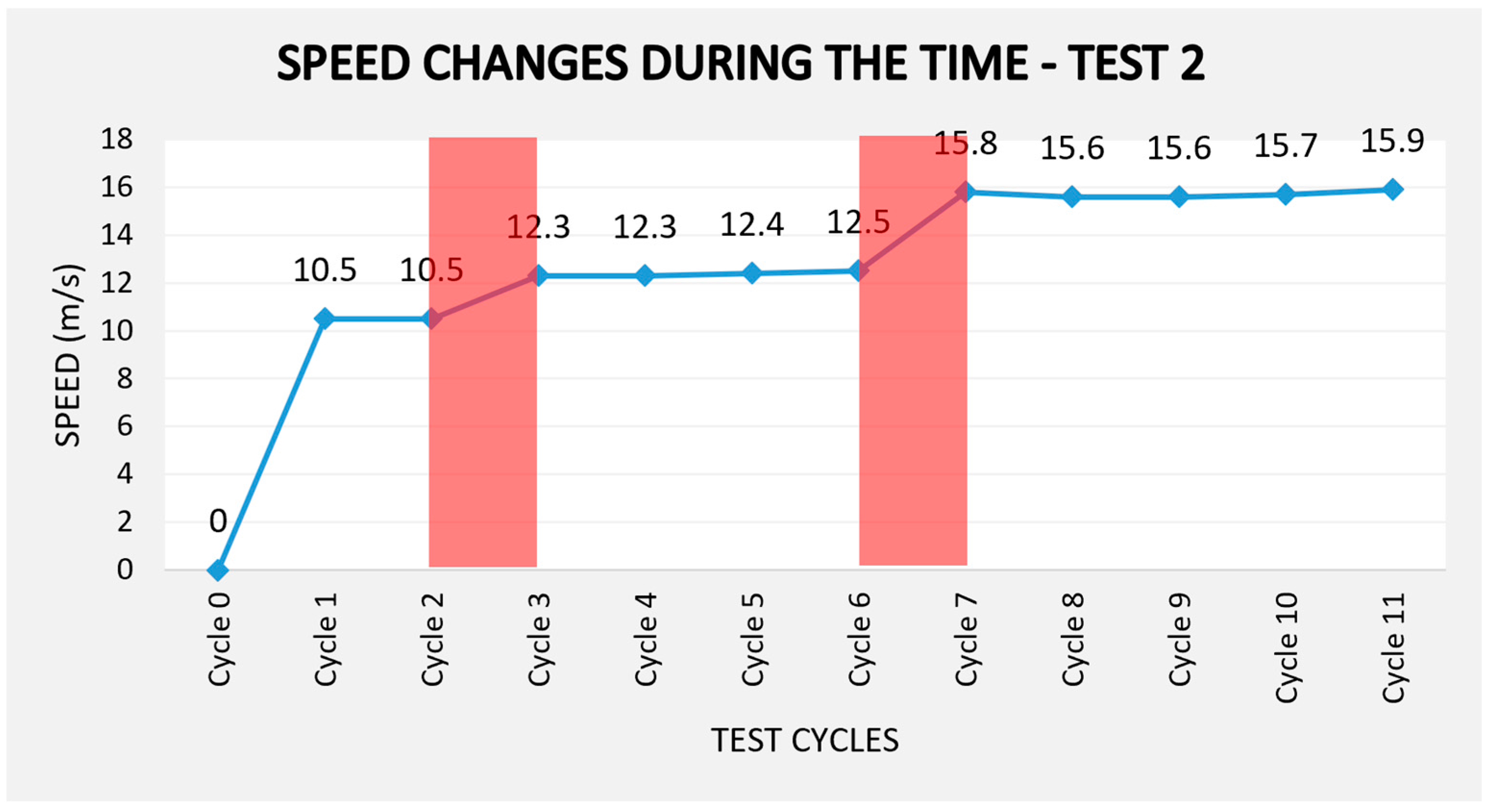
The data presented in Table 3 indicate that conveyor speed adjustments were required at two specific points during the process, occurring in cycles 2 and 6. In the first instances, the adjustment was necessitated by failures in the loading process, which resulted in the conveyor system not transporting any part in cycle 2. In cycle 6, a failure at the intermediate workstation caused a 14 s delay in the cycle approximately.

The simulation model was activated to make speed adjustment, consequently, mitigate the issue. The conveyor, operating autonomously, implemented the new speed parameters to adhere to the predefined production time of 600 s. As a result of these corrective measures, the total duration required to transport all 40 parts was 600.9 s, in addition, one more cycle was required.

Figure 8 illustrates the changes in conveyor speed that occurred on cycles 3 and 7 across work cycles.

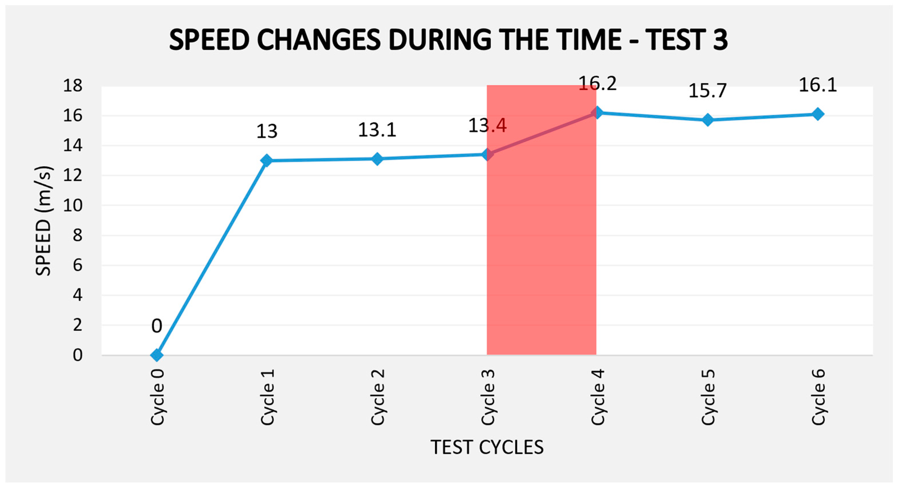
The data presented in Table 4 indicates that conveyor speed adjustments were required when there occurred a failure on cycle 3, in that situation cycle time delay approximately 11 s. The adjustment was necessitated to keep the time process goal, 300 s to transport 24 parts.

Figure 9 illustrates the changes in conveyor speed that occurred on cycle 3 across work cycles.

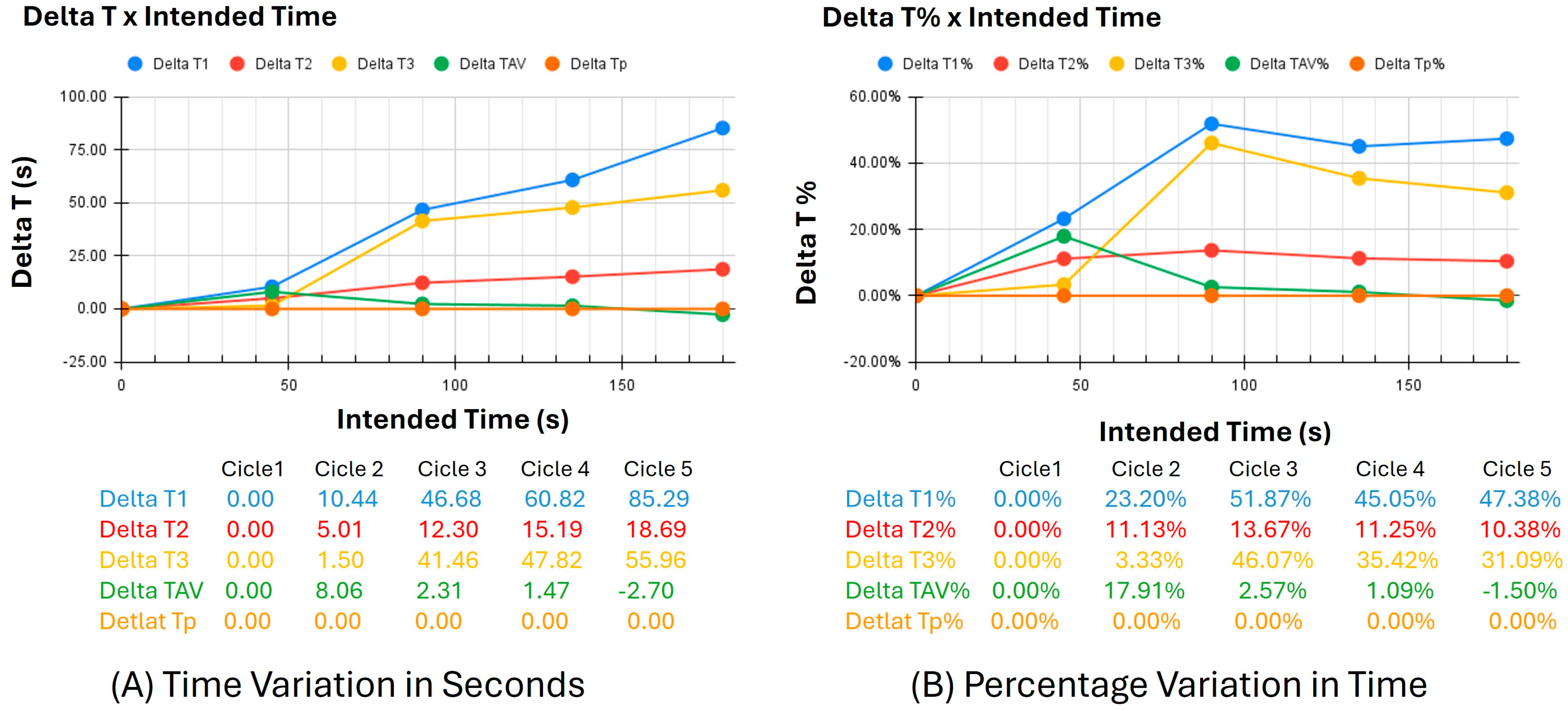
Another test was conducted to analyze the conveyor speed when the cycle time is altered. In this test, the data from the planned cycle time (IT) and the observed cycle times (T1, T2, and T3) were compared, along with the Corrected Cycle Time (TSA).

The charts in Figure 10 illustrate the variations in the test parameters, where chart (A) shows the time variation in seconds, and chart (B) depicts the percentage variation in time. The orange line (Delta IT% and Delta IT) represents the time reference for each of the four cycles analyzed. The blue, yellow, and red lines show the data collected without optimization. The green lines (Delta TSA% and Delta TSA) correspond to the cycles where optimization was applied.

It can be observed that the lines representing the times without optimization exhibit a variation of 47.38% compared to the planned time. Issues occurring in the first two cycles explain this variation. However, it is evident that, despite a 17.91% variation in the first cycle, once speed optimization is applied, the cycle times are closer to the planned values, resulting in only a 1.5% variation from the planned time.

Thus, the application of speed optimization leads to corrections in subsequent work cycles, preventing the accumulation of variations over time.

On the other hand, if the same test were performed without self-reprogramming conditions, additional action would be required to ensure that the production system operates at the necessary speed to prevent delays. In this scenario, failure detection would need to be communicated to the system or the personnel responsible, who would then evaluate the new operating conditions, define the appropriate parameters, and apply the necessary adjustments. Consequently, the production system would continue operating with incorrect parameters for a longer period, exacerbating the issue in proportion to the time required for correction.

In this context, the advantages of developing an integrated system with real-time data exchange become evident, both for problem detection and for transmitting the correct parameters to the production system.

The challenges encountered in this study are indicative of the difficulties that may arise in large-scale applications. The first challenge involves the selection and configuration of sensors responsible for collecting data from the real system. In some cases, sensor signals must be converted into a format compatible with the database to ensure accurate interpretation and storage.

Another critical aspect is the compatibility between different tools. In this prototype, it was necessary to develop a specific code to interpret the collected data and integrate it into the simulation model in a standardized manner. In large-scale applications, the integration of systems such as MES, ERP or RFID will be essential for data exchange with the simulation tool. However, this integration significantly increases the complexity of the development process due to the large volume of data generated.

Finally, the cost of system development and monitoring must be assessed on a case-by-case basis, considering the specific characteristics of the real-world application environment. In highly complex scenarios, excessive costs may compromise the feasibility of the project, highlighting the need for a thorough economic analysis before implementation.

6. Conclusions

Analyzing the results obtained in this study, it can be concluded that the concepts of DT, when applied to a production system, enable the reprogramming of system parameters, allowing operational failures to be resolved autonomously. These results were achieved because the connections established between the real and virtual systems enabled real-time data exchange.

This prototype serves as an initial step toward applying simulation models as a tool for autonomous decision-making and reprogramming of manufacturing systems. Therefore, future work should focus on developing more complex simulation models, incorporating a greater number of variables. As a suggestion, the application of genetic algorithms for problem-solving could prove to be a viable approach.

The application of a tool with the characteristics presented in this prototype can contribute to decision-making support in complex production systems. However, it is essential to conduct a cost-benefit analysis, as the development of a simulation model integrated with the production system depends on the operational capability to collect real-time production data. Moreover, a thorough understanding of the process variables that are critical to the performance of the production system is fundamental. That said, the contribution of this tool to the production system is evident. In the presented tests, it was observed that the autonomous correction of operating variables allowed the initial manufacturing requirements to be met.

This work can serve as a basis for applications in more complex production systems with a greater number of variables, including different manufacturing machines, a wider variety of products, and economic variables arising from the need to meet supply planning for customers.

It is recommended that this work be applied to production systems with discrete characteristics. Furthermore, a study should be conducted to evaluate the impact of workers when implementing this technology under real working conditions.