
Numerical Evaluation of the Equivalent Damping Ratio Due to Dissipative Roof Structure in the Retrofit of Historical Churches


Abstract
1. Introduction
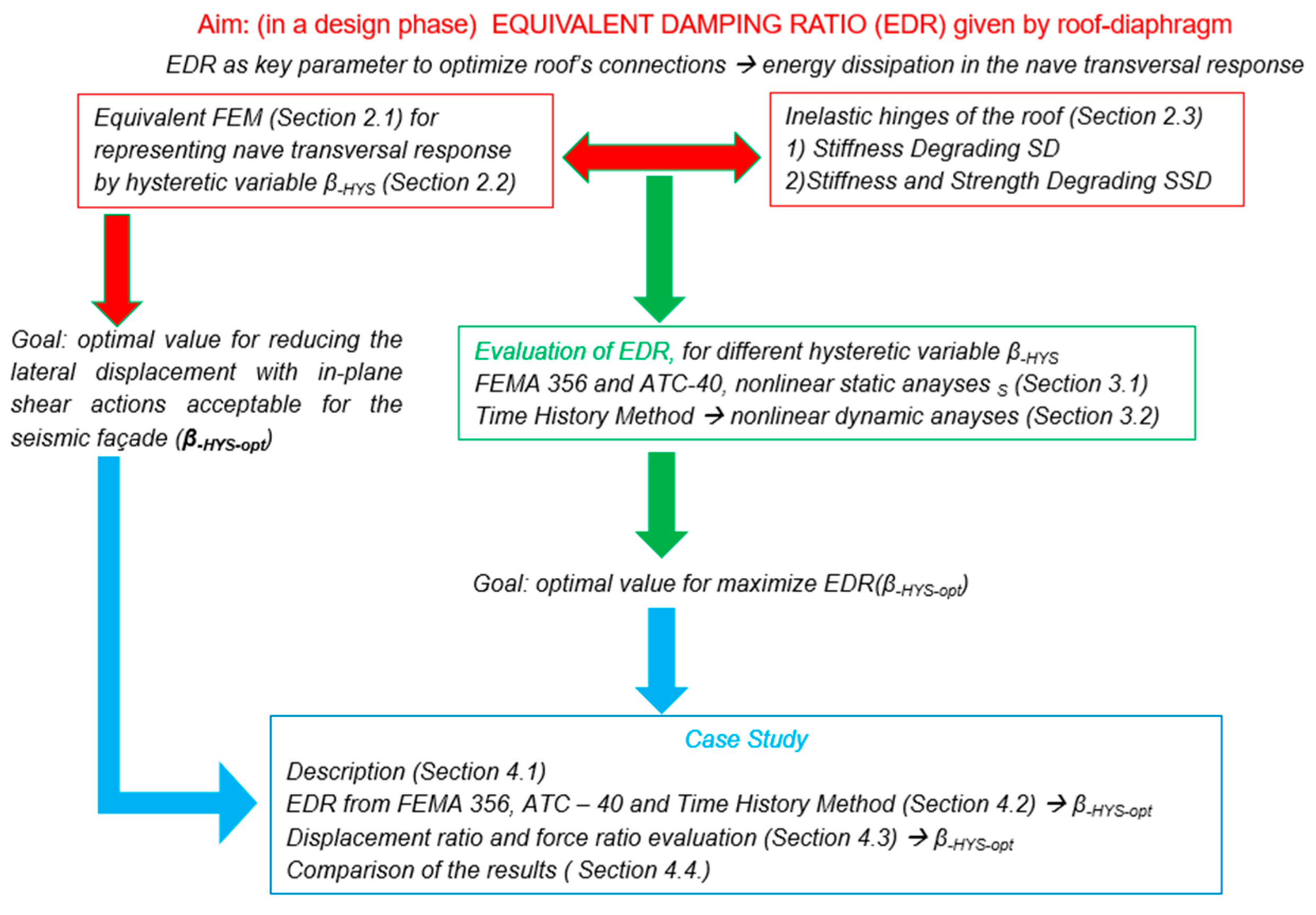
2. Simulation of the Nave Transversal Response by Equivalent FEM
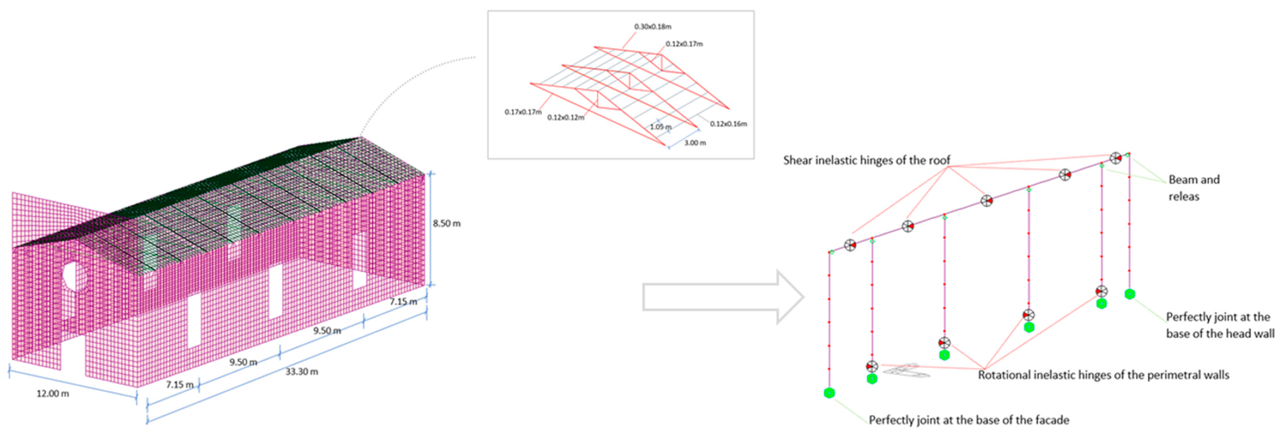
2.1. Equivalent FEM
2.2. Simulation of the Nave Transversal Response
- nws is the homogenization coefficient of the steel-to-wooden diaphragm connection, given by nws = Es/Ew* (where Es is the steel elastic modulus);
- L is the distance between the seismic-resistant elements (the spacing between the transversal frames);
- Ly is the width of the roof;
- i is the spacing of the connectors;
- kn is the stiffness of a single connector;
- tw is the thickness of the wooden panels;
- χ = 6/5cos2α is the shear factor of the cross-section (χ = 1.2 for rectangular sections);
- Aw is the cross-section area of the roof diaphragm;
- A* is the shear area given by Equation (10), as follows:
- nn is the number of connectors for each connection stripe (the ratio between the spacing of the seismic elements and the spacing of the connectors);
- ns is the number of the connection stripes for each span;
- As is the cross-section area of the thin steel stripes of the roof diaphragm.
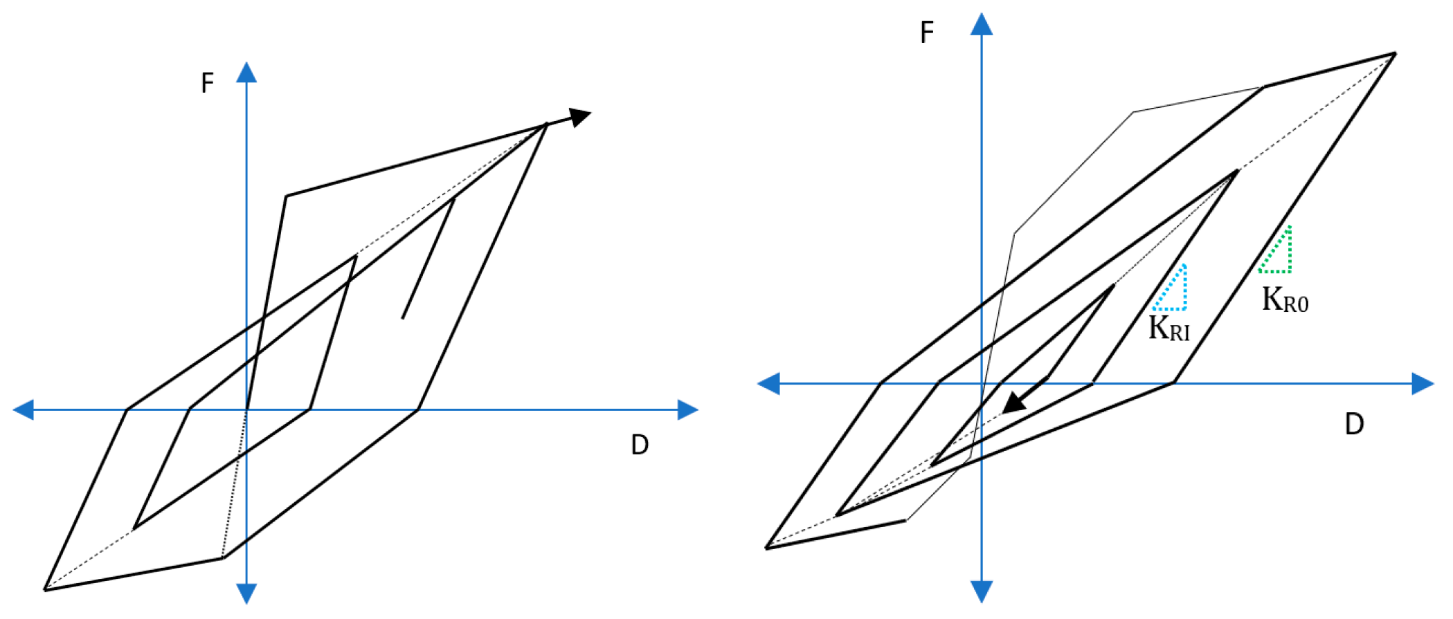
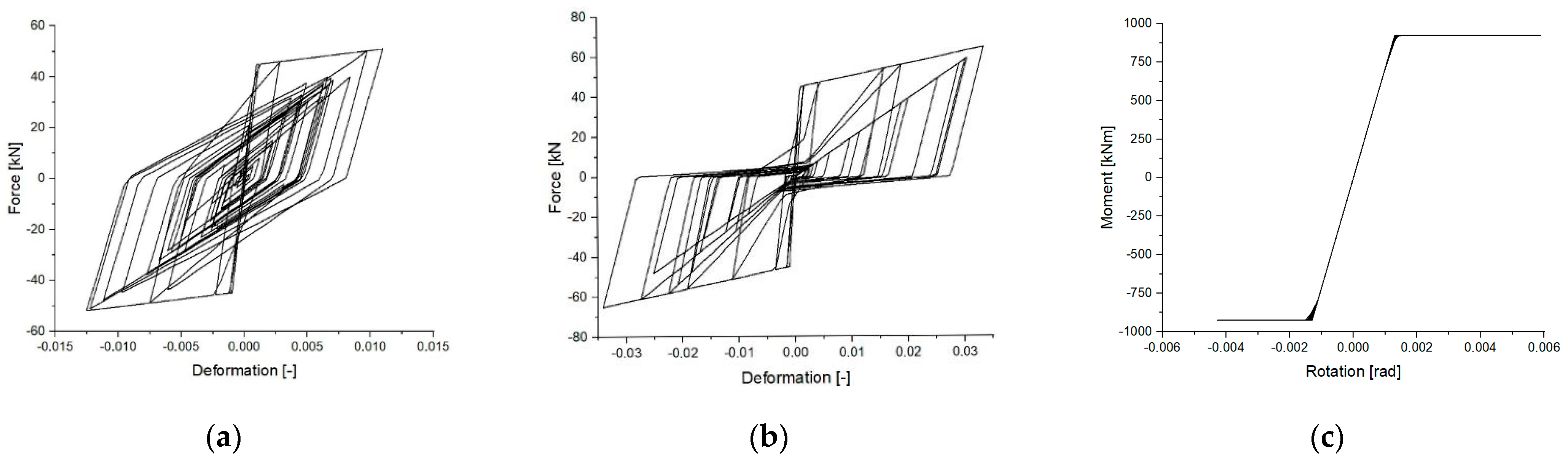
2.3. Hysteretic Models for the Roof’s Connections
3. Methods for EDR Evaluation
3.1. Equivalent Damping Ratio (EDR) in Capacity Sptectrum Method (CSM)
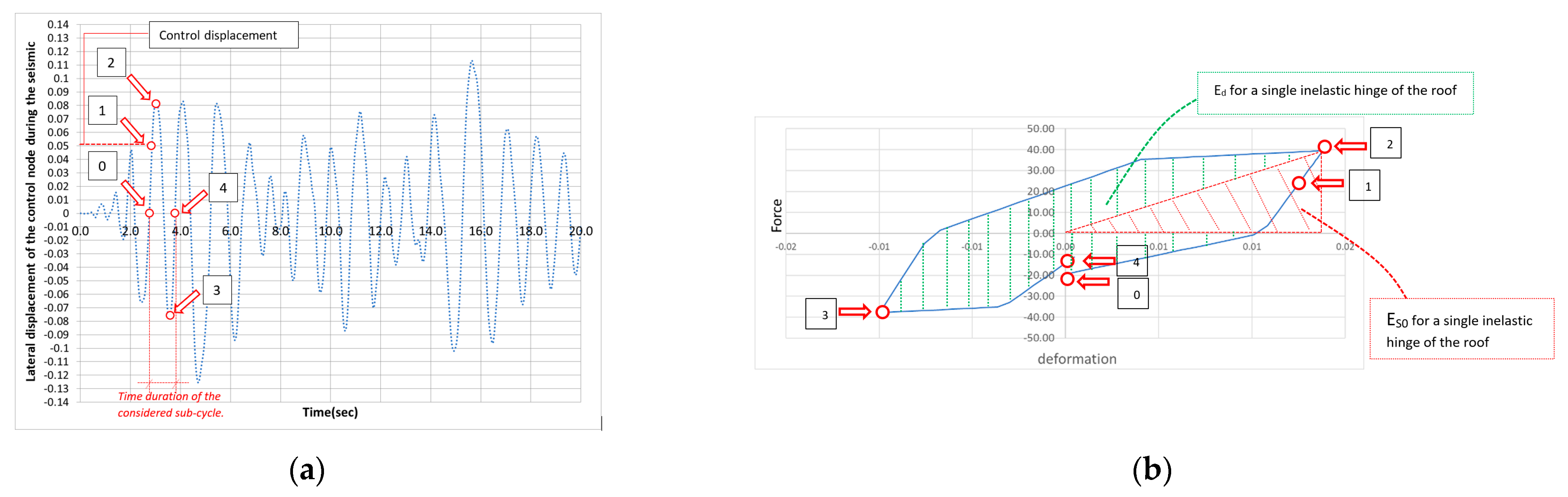
3.2. Time History Method for EDR Evaluation
4. Case Study
4.1. Description of the Case Study
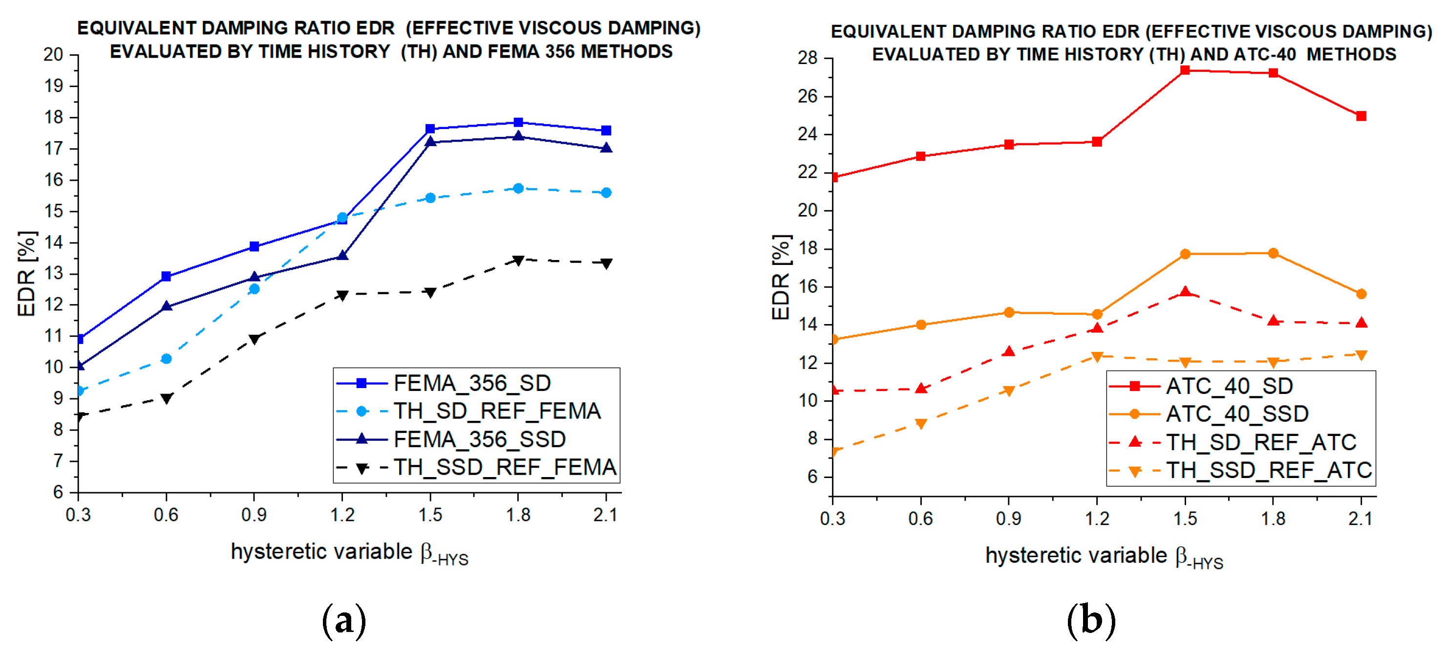
4.2. Results in Terms of EDR
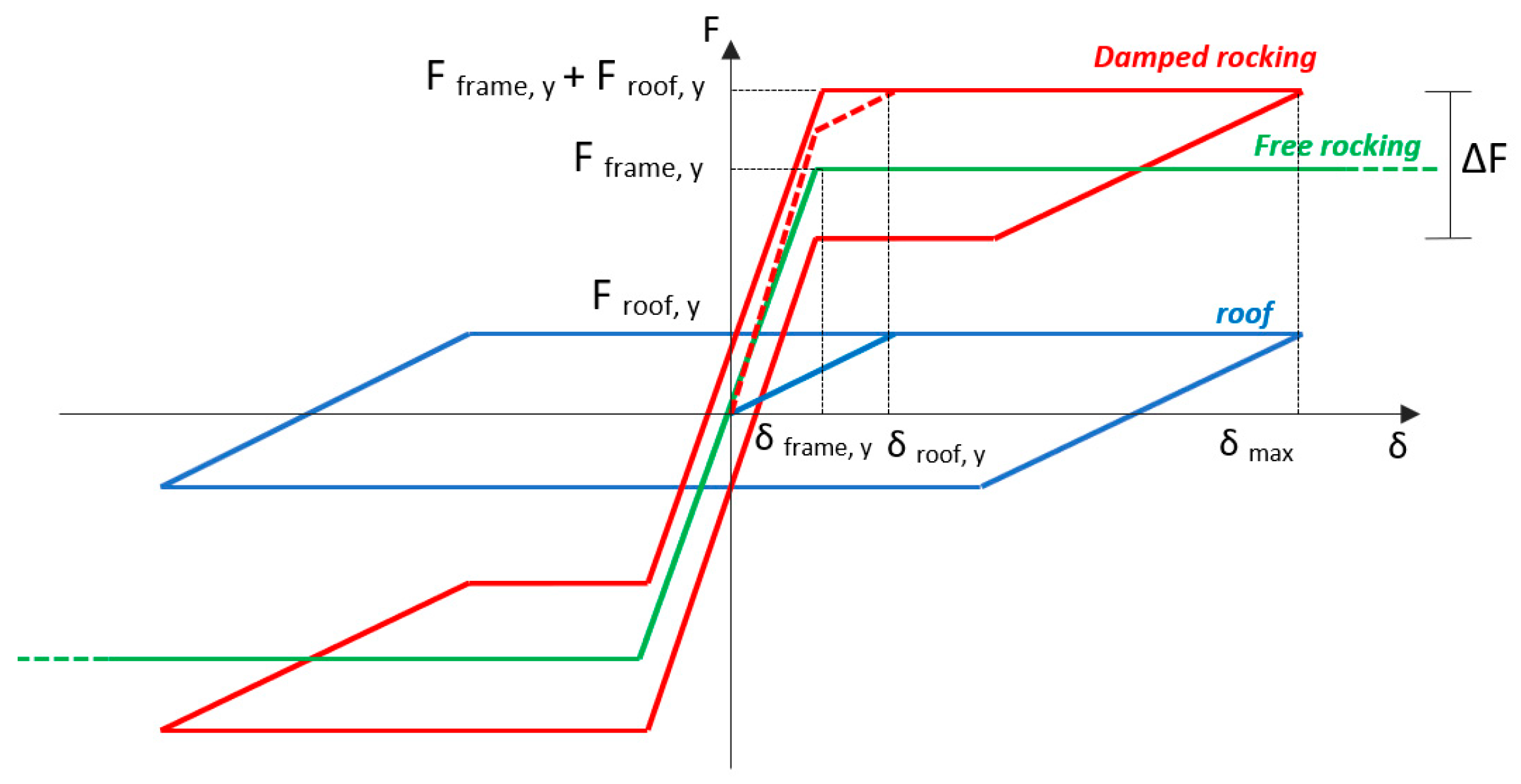
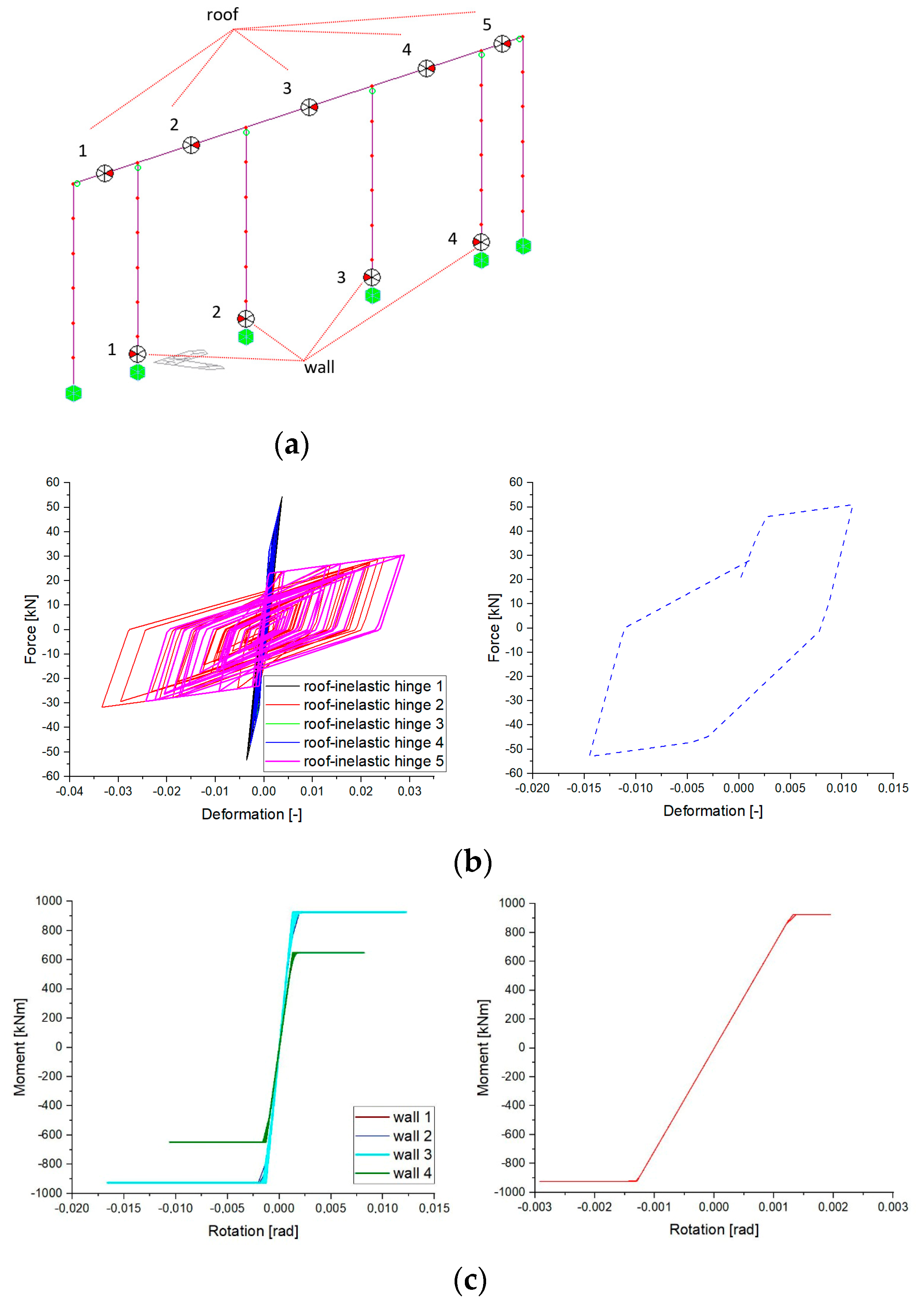
4.3. Results in Terms of Damped Rocking
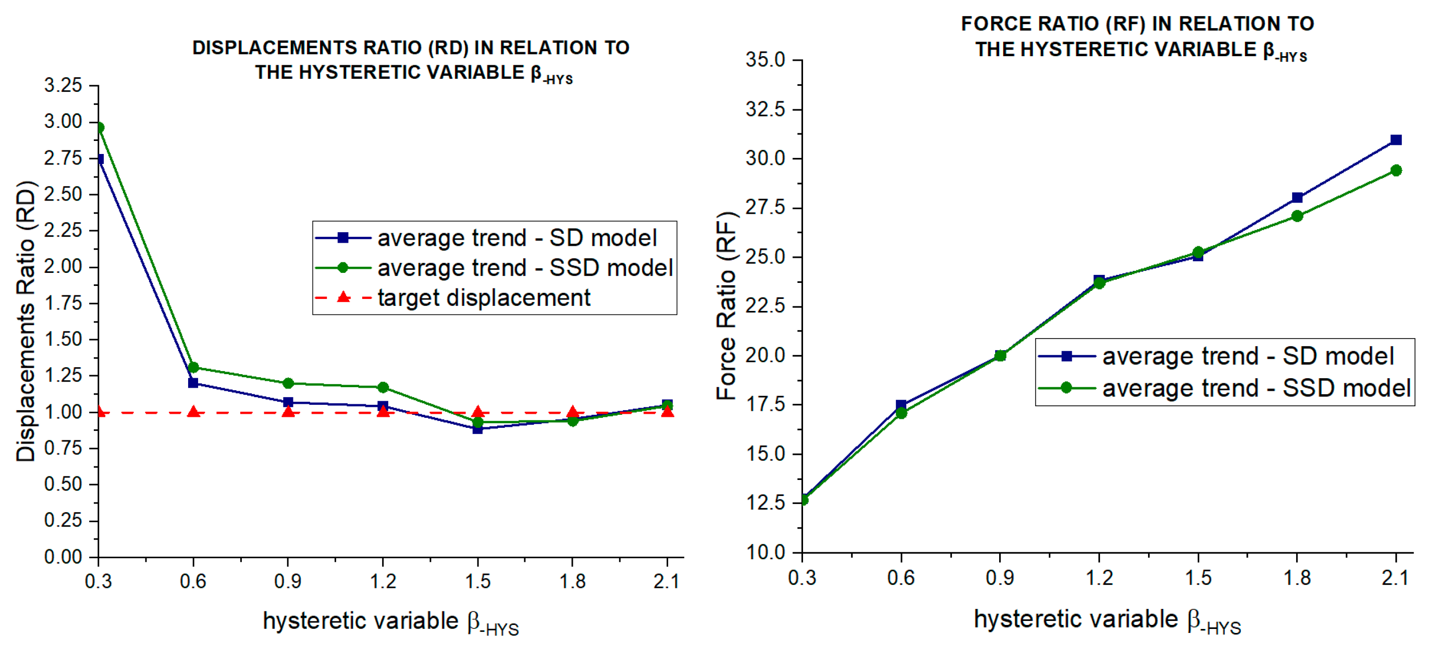
- The RF is the ratio between the shear force evaluated in the node connecting the roof to the façade in the equivalent FEM, and the total shear force evaluated at the base of the structure;
- The RD is defined as the ratio between the transversal displacement of the roof and the target displacement (chosen as the 0.5% of the total height of the perimeter walls).
4.4. Remarks
5. Conclusions
- The equivalent FEM is useful to define the roof design during the preliminary design phase;
- The analyses performed with the equivalent FEM represent a fast method to define the roof configuration that best achieves a global box behavior in seismic response;
- The performed analyses allow us to test different possible retrofitted roof configurations through various values of the hysteretic variable. On the contrary, during the conceptual design phase, the analysis of local mechanisms (also referred to as macro-elements) or the implementation of 3D models represent the standard approach to evaluate the capacity of the original construction;
- By performing nonlinear dynamic analyses, the EDR and the transversal drift of the roof are characterized by a similar variation as a function of the hysteretic variable β-HYS;
- The TH approach gives EDR values lower than those evaluated by the PO analyses performed according to FEMA 356 and ATC-40;
- The effects of the SD and SSD hysteretic models are significant in terms of the dissipated energy during the seismic event;
- ATC-40 overestimates the EDR values, especially if the SD model is adopted;
- The optimal β-HYS-opt value detected in the transversal displacement diagram is also valid for the EDR estimation;
- For a hysteretic variable β-HYS greater than 1.5, the dissipative effect of the roof diaphragm no longer increases, indicating that the structural configuration becomes excessively rigid beyond this limit.
Author Contributions
Funding
Institutional Review Board Statement
Informed Consent Statement
Data Availability Statement
Acknowledgments
Conflicts of Interest
References
- Milani, G. Lesson Learned after the Emilia-Romagna, Italy, 20-29 May 2012 Earthquakes: A Limit Analysis Insight on Three Masonry Churches. Eng. Fail. Anal. 2013, 34, 761–778. [Google Scholar] [CrossRef]
- Liberatore, D.; Doglioni, C.; AlShawa, O.; Atzori, S.; Sorrentino, L. Effects of Coseismic Ground Vertical Motion on Masonry Constructions Damage during the 2016 Amatrice-Norcia (Central Italy) Earthquakes. Soil Dyn. Earthq. Eng. 2019, 120. [Google Scholar] [CrossRef]
- Longarini, N.; Crespi, P.; Zucca, M. The Influence of the Geometrical Features on the Seismic Response of Historical Churches Reinforced by Different Cross Lam Roof-Solutions. Bull. Earthq. Eng. 2022, 20, 6813–6852. [Google Scholar] [CrossRef]
- Longarini, N.; Crespi, P.; Scamardo, M. Numerical Approaches for Cross-Laminated Timber Roof Structure Optimization in Seismic Retrofitting of a Historical Masonry Church. Bull. Earthq. Eng. 2020, 18, 487–512. [Google Scholar] [CrossRef]
- Parisi, M.A.; Tardini, C. Seismic Vulnerability Assessment of Timber Roof Structures: Criteria and Procedures. Proc. Inst. Civil. Eng. Struct. Build. 2021, 174, 431–442. [Google Scholar] [CrossRef]
- Giuriani, E.P.; Marini, A.; Preti, M. Thin-Folded Shell for the Renewal of Existing Wooden Roofs. Int. J. Archit. Herit. 2016, 10, 797–816. [Google Scholar] [CrossRef]
- Department of Homeland Security. FEMA 440: Improvement of Nonlinear Static Seismic Analysis Procedures; Department of Homeland Security: Washington, DC, USA, 2005.
- Castellazzi, G.; Gentilini, C.; Nobile, L. Seismic Vulnerability Assessment of a Historical Church: Limit Analysis and Nonlinear Finite Element Analysis. Adv. Civil. Eng. 2013, 2013, 517454. [Google Scholar] [CrossRef]
- Micelli, F.; Cascardi, A. Structural Assessment and Seismic Analysis of a 14th Century Masonry Tower. Eng. Fail. Anal. 2020, 107, 104198. [Google Scholar] [CrossRef]
- Shehu, R. Preliminary Assessment of the Seismic Vulnerability of Three Inclined Bell-Towers in Ferrara, Italy. Int. J. Archit. Herit. 2022, 16, 485–517. [Google Scholar] [CrossRef]
- de Silva, F.; Ceroni, F.; Sica, S.; Silvestri, F. Non-Linear Analysis of the Carmine Bell Tower under Seismic Actions Accounting for Soil–Foundation–Structure Interaction. Bull. Earthq. Eng. 2018, 16, 2775–2808. [Google Scholar] [CrossRef]
- Preciado, A. Seismic Vulnerability and Failure Modes Simulation of Ancient Masonry Towers by Validated Virtual Finite Element Models. Eng. Fail. Anal. 2015, 57, 72–87. [Google Scholar] [CrossRef]
- Cannizzaro, F.; Pantò, B.; Lepidi, M.; Caddemi, S.; Caliò, I. Multi-Directional Seismic Assessment of Historical Masonry Buildings by Means of Macro-Element Modelling: Application to a Building Damaged during the L’Aquila Earthquake (Italy). Buildings 2017, 7, 106. [Google Scholar] [CrossRef]
- Masciotta, M.G.; Lourenço, P.B. Seismic Analysis of Slender Monumental Structures: Current Strategies and Challenges. Appl. Sci. 2022, 12, 7340. [Google Scholar] [CrossRef]
- Yu, L.L.; Dong, Z.Q.; Li, G. Simplified Mechanical Models for the Seismic Collapse Performance Prediction of Unreinforced Masonry Structures. Eng. Struct. 2022, 258, 114131. [Google Scholar] [CrossRef]
- Xiang, M.; Shen, J.; Xu, Z.; Chen, J. Structure-to-structure Seismic Damage Correlation Model. Earthq. Eng. Struct. Dyn. 2024, 53, 3205–3229. [Google Scholar] [CrossRef]
- Preti, M.; Loda, S.; Bolis, V.; Cominelli, S.; Marini, A.; Giuriani, E. Dissipative Roof Diaphragm for the Seismic Retrofit of Listed Masonry Churches. J. Earthq. Eng. 2019, 23, 1241–1261. [Google Scholar] [CrossRef]
- Preti, M.; Bolis, V.; Marini, A.; Giuriani, E. Example of the Benefits of a Dissipative Roof Diaphragm in the Seismic Response of Masonry. In Proceedings of the SAHC2014–9th International Conference on Structural Analysis of Historical Constructions, Mexico City, Mexico, 4–17 October 2014. [Google Scholar]
- Alvares da Silva, A.H.; Stojadinović, B. Surrogate Models for Seismic Response Analysis of Flexible Rocking Structures. Earthq. Eng. Struct. Dyn. 2024, 53, 3701–3725. [Google Scholar] [CrossRef]
- Ceccotti, A.; Sandhaas, C.; Okabe, M.; Yasumura, M.; Minowa, C.; Kawai, N. SOFIE Project—3D Shaking Table Test on a Seven-Storey Full-Scale Cross-Laminated Timber Building. Earthq. Eng. Struct. Dyn. 2013, 42, 2003–2021. [Google Scholar] [CrossRef]
- Valdivieso, D.; Almazán, J.L.; Lopez-Garcia, D.; Montaño, J.; Liel, A.B.; Guindos, P. System Effects in T-shaped Timber Shear Walls: Effects of Transverse Walls, Diaphragms, and Axial Loading. Earthq. Eng. Struct. Dyn. 2024, 53, 2532–2554. [Google Scholar] [CrossRef]
- Johansen, K.W. Theory of Timber Connections; IABSE: International Association of Bridge and Structural Engineering: Zurich, Switzerland, 1949; Volume 9. [Google Scholar]
- Shahnewaz, M.; Alam, S.; Tannert, T. In-Plane Strength and Stiffness of Cross-Laminated Timber Shear Walls. Buildings 2018, 8, 100. [Google Scholar] [CrossRef]
- Sandhaas, C.; van de Kuilen, J.W.G. Strength and Stiffness of Timber Joints with Very High Strength Steel Dowels. Eng. Struct. 2017, 131, 394–404. [Google Scholar] [CrossRef]
- Hossain, A.; Lakshman, R.; Tannert, T. Shear Connections with Self-Tapping Screws for Cross-Laminated Timber Panels. In Proceedings of the Structures Congress 2015, Portland, OR, USA, 23–25 April 2015. [Google Scholar]
- EN 1995-1-1; Eurocode 5—Design of Timber Structures—General—Common Rules and Rules for Buildings. CEN: Brussels, Belgium, 2004; Volume 144.
- Aloisio, A.; Alaggio, R.; Fragiacomo, M. Equivalent Viscous Damping of Cross-Laminated Timber Structural Archetypes. J. Struct. Eng. 2021, 147, 04021012. [Google Scholar] [CrossRef]
- Barbosa, M.J.; Pauwels, P.; Ferreira, V.; Mateus, L. Towards Increased BIM Usage for Existing Building Interventions. Struct. Surv. 2016, 34, 168–190. [Google Scholar] [CrossRef]
- Federal Emergency Management Agency. Prestandard and Commentary for the Seismic Rehabilitation of Buildings; FEMA 356; Federal Emergency Management Agency: Washington, DC, USA, 2000.
- Applied Technology Council. ATC 40, Seismic Evaluation and Retrofit of Concrete Buildings; Seismic Safety Commission: West Sacramento, CA, USA, 1996; Volume 1.
- Habieb, A.B.; Valente, M.; Milani, G. Base Seismic Isolation of a Historical Masonry Church Using Fiber Reinforced Elastomeric Isolators. Soil Dyn. Earthq. Eng. 2019, 120, 127–145. [Google Scholar] [CrossRef]
- Valente, M.; Barbieri, G.; Biolzi, L. Seismic Assessment of Two Masonry Baroque Churches Damaged by the 2012 Emilia Earthquake. Eng. Fail. Anal. 2017, 79, 773–802. [Google Scholar] [CrossRef]
- Valente, M.; Barbieri, G.; Biolzi, L. Damage Assessment of Three Medieval Churches after the 2012 Emilia Earthquake. Bull. Earthq. Eng. 2017, 15, 2939–2980. [Google Scholar] [CrossRef]
- Cacciola, P.; Deodatis, G. A Method for Generating Fully Non-Stationary and Spectrum-Compatible Ground Motion Vector Processes. Soil Dyn. Earthq. Eng. 2011, 31, 351–360. [Google Scholar] [CrossRef]
- Iervolino, I.; Galasso, C.; Cosenza, E. REXEL: Computer Aided Record Selection for Code-Based Seismic Structural Analysis. Bull. Earthq. Eng. 2010, 8, 339–362. [Google Scholar] [CrossRef]
- Giuriani, E.; Marini, A. Wooden Roof Box Structure for the Anti-Seismic Strengthening of Historic Buildings. Int. J. Archit. Herit. 2008, 2, 226–246. [Google Scholar] [CrossRef]
- Preti, M.; Bolis, V.; Giuriani, E.; Marini, A.; Peretti, M. Studio Del Ruolo Del Diaframma Di Copertura Nel Comportamento Sismico Degli Archi Diaframma Nella Chiesa Parrocchiale Di Sirmione; Technical Report n. 1; Università di Brescia: Brescia, Italy, 2013. [Google Scholar]
- Genshu, T.; Yongfeng, Z. Seismic Force Modification Factors for Modified-Clough Hysteretic Model. Eng. Struct. 2007, 29, 3053–3070. [Google Scholar] [CrossRef]
- Loss, C.; Hossain, A.; Tannert, T. Simple Cross-Laminated Timber Shear Connections with Spatially Arranged Screws. Eng. Struct. 2018, 173, 340–356. [Google Scholar] [CrossRef]
- Iwan, W.D.; Gates, N.C. The Effective Period and Damping of a Class of Hysteretic Structures. Earthq. Eng. Struct. Dyn. 1979, 7, 199–211. [Google Scholar] [CrossRef]
- Clough, R.W. Effect of Stiffness Degradation on Earthquake Ductility Requirements; UC Berkeley: Berkeley, CA, USA, 1966. [Google Scholar]
- Otani, S. Hysteresis models of reinforced concrete for earthquake response analysis. J. Fac. Eng. Univ. Tokyo Ser. B 1981, 36, 125–159. [Google Scholar]
- Takeda, T.; Sozen, M.A.; Nielsen, N.N. Reinforced Concrete Response to Simulated Earthquakes. J. Struct. Div. 1970, 96, 2557–2573. [Google Scholar] [CrossRef]
- Jacobsen, L. Steady Forced Vibrations as Influenced by Damping. Trans. Am. Soc. Mech. Eng. 1930, 52, 169–181. [Google Scholar] [CrossRef]
- Jacobsen, L. Damping in Composite Structures. In Proceedings of the 2nd World Conference on on Earthquake Engineering, Tokyo and Kyoto, Japan, 11–18 July 1960; Volume 2. [Google Scholar]
- Jennings, P.C. Equivalent Viscous Damping for Yielding Structures. J. Eng. Mech. Div. 1968, 94, 103–116. [Google Scholar] [CrossRef]
- Laguardia, R.; Franchin, P.; Tesfamariam, S. Risk-Based Optimization of Concentrically Braced Tall Timber Buildings: Derivative Free Optimization Algorithm. Earthq. Eng. Struct. Dyn. 2024, 53, 179–199. [Google Scholar] [CrossRef]
- Priestley, M.J.N. Myths and Fallacies in Earthquake Engineering, Revisited: The Ninth Mallet Milne Lecture; IUSS Press: Pavia, Italy, 2003. [Google Scholar]
- Chopra, A.K. Dynamics of Structures; Pearson Education: London, UK, 2019. [Google Scholar]
- Elmenshawi, A.; Sorour, M.; Mufti, A.; Jaeger, L.G.; Shrive, N. Damping Mechanisms and Damping Ratios in Vibrating Unreinforced Stone Masonry. Eng. Struct. 2010, 32, 3269–3278. [Google Scholar] [CrossRef]
- Lubliner, J.; Oliver, J.; Oller, S.; Oñate, E. A Plastic-Damage Model for Concrete. Int. J. Solids Struct. 1989, 25, 299–326. [Google Scholar] [CrossRef]
- Lee, J.; Fenves, G.L. Plastic-Damage Model for Cyclic Loading of Concrete Structures. J. Eng. Mech. 1998, 124, 892–900. [Google Scholar] [CrossRef]
- Valente, M.; Milani, G. Damage Assessment and Partial Failure Mechanisms Activation of Historical Masonry Churches under Seismic Actions: Three Case Studies in Mantua. Eng. Fail. Anal. 2018, 92, 495–519. [Google Scholar] [CrossRef]
- Midas GEN 2023. Available online: https://support.midasuser.com/hc/en-us/articles/27773333780761--GEN-2023-v1-1-Release-Note (accessed on 30 January 2025).
- Dong, H.; He, M.; Wang, X.; Christopoulos, C.; Li, Z.; Shu, Z. Development of a Uniaxial Hysteretic Model for Dowel-Type Timber Joints in OpenSees. Constr. Build. Mater. 2021, 288, 123112. [Google Scholar] [CrossRef]
- Hong, J.-P.; Barrett, D. Three-Dimensional Finite-Element Modeling of Nailed Connections in Wood. J. Struct. Eng. 2010, 136, 715–722. [Google Scholar] [CrossRef]
- He, M.; Lam, F.; Foschi, R.O. Modeling Three-Dimensional Timber Light-Frame Buildings. J. Struct. Eng. 2001, 127, 901–913. [Google Scholar] [CrossRef]
- Totani, G.; Monaco, P.; Totani, F.; Lanzo, G.; Pagliaroli, A.; Amoroso, S.; Marchetti, D. Site Characterization and Seismic Response Analysis in the Area of Collemaggio, L’Aquila (Italy). In Proceedings of the 5th International Conference on Geotechnical and Geophysical Site Characterisation, ISC 2016, Gold Coast, Australia, 5–9 September 2016; Volume 2. [Google Scholar]
- NTC2018, I.M. of I. Norme Tecniche per Le Costruzioni. DM 17/1/2018 (In Italian). Gazzetta Ufficiale della Repubblica Italiana. 2018. Available online: https://biblus.acca.it/download/norme-tecniche-per-le-costruzioni-2018-ntc-2018-pdf/ (accessed on 30 January 2025).


| Parts of the Roof Close to the Head Wall and Facade | |||||||
|---|---|---|---|---|---|---|---|
| β-HYS | P1 [kN] = Froof,y | P2 [kN] = Froof,u | D1 = (P1/Kroof,y)/L | D2 | Mframe,y = Mframe,u [kNm] | Rframe,y [rad] | Rframe,u [rad] |
| 0.30 | 9.69 | 12.11 | 0.00062 | 0.01257 | 555.422 | 0.00086 | 0.00258 |
| 0.60 | 19.38 | 24.22 | 0.00062 | 0.01257 | 555.422 | 0.00086 | 0.00258 |
| 0.90 | 29.06 | 36.33 | 0.00062 | 0.01257 | 555.422 | 0.00086 | 0.00258 |
| 1.20 | 38.75 | 48.44 | 0.00062 | 0.01257 | 555.422 | 0.00086 | 0.00258 |
| 1.50 | 48.44 | 60.55 | 0.00062 | 0.01257 | 555.422 | 0.00086 | 0.00258 |
| 1.80 | 58.13 | 72.66 | 0.00062 | 0.01257 | 555.422 | 0.00086 | 0.00258 |
| 2.10 | 67.81 | 84.77 | 0.00062 | 0.01257 | 555.422 | 0.00086 | 0.00258 |
| Central Parts of the Roof | |||||||
| β-HYS | P1 [kN] = Froof,y | P2 [kN] = Froof,u | D1 = (P1/Kroof,y)/L | D2 | Mframe,y= Mframe,u [kNm] | Rframe,y [rad] | Rframe,u [rad] |
| 0.30 | 189.72 | 237.15 | 0.008619834 | 0.17239 | 10,877.185 | 0.01182 | 0.03548 |
| 0.60 | 379.44 | 474.30 | 0.008619834 | 0.17239 | 10,877.185 | 0.01182 | 0.03548 |
| 0.90 | 569.16 | 711.44 | 0.008619834 | 0.17239 | 10,877.185 | 0.01182 | 0.03548 |
| 1.20 | 758.87 | 948.59 | 0.008619834 | 0.17239 | 10,877.185 | 0.01182 | 0.03548 |
| 1.50 | 948.59 | 1185.74 | 0.008619834 | 0.17239 | 10,877.185 | 0.01182 | 0.03548 |
| 1.80 | 1138.31 | 1422.89 | 0.008619834 | 0.17239 | 10,877.185 | 0.01182 | 0.03548 |
| 2.10 | 1328.03 | 1660.04 | 0.008619834 | 0.17239 | 10,877.185 | 0.01182 | 0.03548 |
| β-HYS | Method | SD—Target Displacement [m] | SSD—Target Displacement [m] |
|---|---|---|---|
| 0.3 | PO-FEMA/PO-ATC | 0.038/0.055 | 0.041/0.057 |
| 0.6 | PO-FEMA/PO-ATC | 0.028/0.051 | 0.030/0.056 |
| 0.9 | PO-FEMA/PO-ATC | 0.028/0.044 | 0.031/0.050 |
| 1.2 | PO-FEMA/PO-ATC | 0.027/0.045 | 0.030/0.050 |
| 1.5 | PO-FEMA/PO-ATC | 0.037/0.054 | 0.039/0.057 |
| 1.8 | PO-FEMA/PO-ATC | 0.036/0.051 | 0.035/0.050 |
| 2.1 | PO-FEMA/PO-ATC | 0.021/0.039 | 0.021/0.039 |
| Mode | Period | tran-x | tran-y | rotn-z | |||
|---|---|---|---|---|---|---|---|
| n.° | [s] | Mass (%) | Sum (%) | Mass (%) | Sum (%) | Mass (%) | Sum (%) |
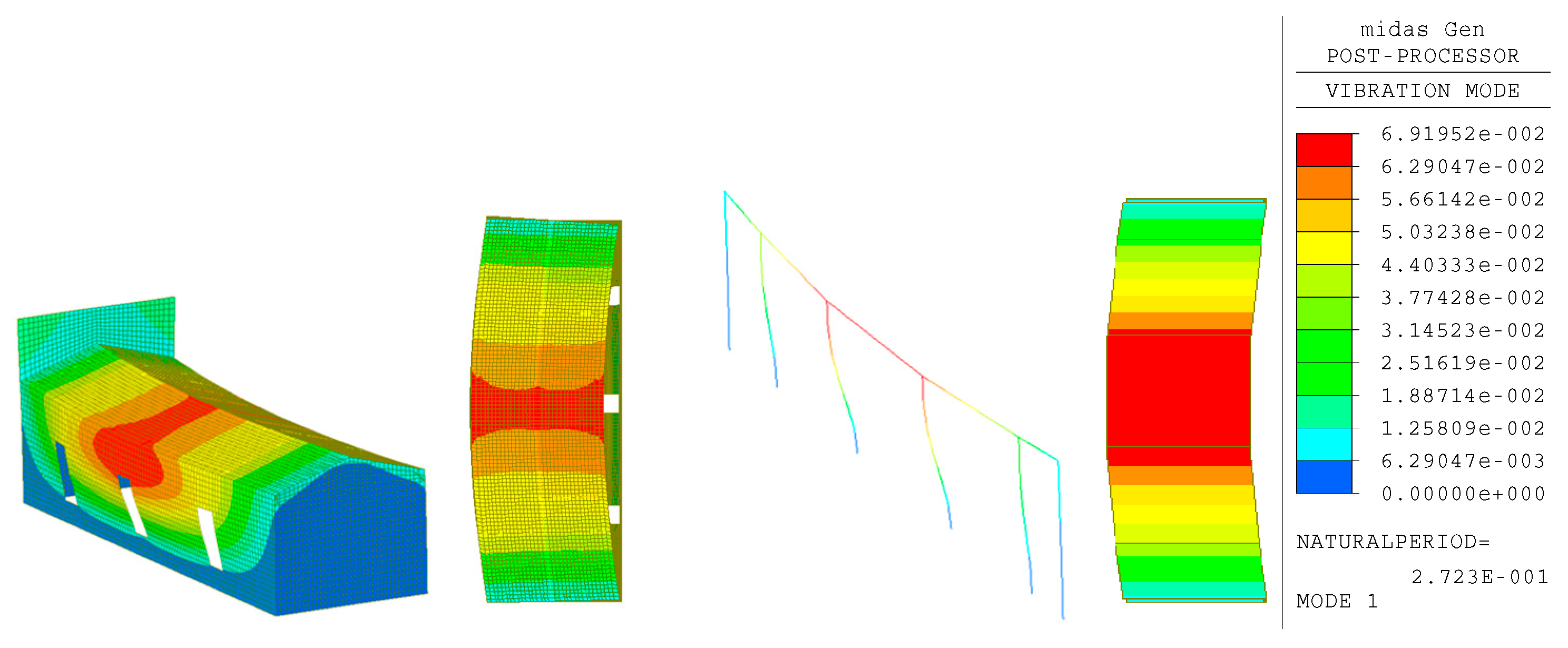
| 1 | 0.271 | 58.54 | 58.54 | 0.00 | 0.00 | 0.03 | 0.03 |
| 2 | 0.185 | 0.00 | 58.54 | 39.78 | 39.78 | 0.00 | 0.03 |
| 3 | 0.183 | 0.13 | 58.67 | 0.00 | 39.78 | 39.12 | 39.15 |
| 4 | 0.179 | 0.00 | 58.67 | 0.07 | 39.85 | 0.00 | 39.15 |
| 5 | 0.175 | 5.96 | 64.63 | 0.00 | 39.85 | 0.05 | 39.20 |
| 6 | 0.174 | 0.01 | 64.64 | 0.00 | 39.85 | 4.00 | 43.20 |
| 7 | 0.123 | 2.25 | 66.89 | 0.00 | 39.85 | 0.00 | 43.20 |
| 8 | 0.116 | 0.00 | 66.89 | 35.40 | 75.25 | 0.00 | 43.20 |
| 9 | 0.092 | 0.01 | 66.91 | 0.00 | 75.25 | 24.12 | 67.33 |
| 10 | 0.076 | 15.19 | 82.09 | 0.00 | 75.25 | 0.30 | 67.63 |
| 11 | 0.073 | 0.00 | 82.09 | 0.01 | 75.26 | 0.00 | 67.63 |
| 12 | 0.063 | 0.01 | 82.11 | 0.00 | 75.26 | 8.41 | 76.04 |
| 13 | 0.057 | 0.00 | 82.11 | 7.01 | 82.27 | 0.00 | 76.04 |
| 14 | 0.056 | 2.37 | 84.48 | 0.00 | 82.27 | 5.17 | 81.20 |
| 15 | 0.055 | 3.05 | 87.53 | 0.00 | 82.27 | 5.62 | 86.82 |
| 16 | 0.055 | 0.00 | 87.53 | 0.02 | 82.29 | 0.00 | 86.82 |
| 17 | 0.051 | 0.00 | 87.53 | 0.45 | 82.74 | 0.00 | 86.82 |
| 18 | 0.050 | 3.23 | 90.76 | 0.00 | 82.74 | 0.01 | 86.83 |
| 19 | 0.048 | 0.00 | 90.76 | 0.00 | 82.74 | 0.00 | 86.83 |
| 20 | 0.047 | 0.00 | 90.76 | 0.00 | 82.74 | 0.00 | 86.83 |
| Method | Model | EDR [%] |
|---|---|---|
| FEMA 356 | SD | ≃16.8 |
| ATC-40 | SD | ≃25.0 |
| TH in relation to FEMA 356 | SD | ≃15.2 |
| TH in relation to ATC-40 | SD | ≃14.8 |
| FEMA 356 | SSD | ≃16.0 |
| ATC-40 | SSD | ≃16.3 |
| TH in relation to FEMA 356 | SSD | ≃12.5 |
| TH in relation to ATC-40 | SSD | ≃12.1 |
Disclaimer/Publisher’s Note: The statements, opinions and data contained in all publications are solely those of the individual author(s) and contributor(s) and not of MDPI and/or the editor(s). MDPI and/or the editor(s) disclaim responsibility for any injury to people or property resulting from any ideas, methods, instructions or products referred to in the content. |
© 2025 by the authors. Licensee MDPI, Basel, Switzerland. This article is an open access article distributed under the terms and conditions of the Creative Commons Attribution (CC BY) license (https://creativecommons.org/licenses/by/4.0/).
Share and Cite
Longarini, N.; Crespi, P.; Zucca, M.; Scamardo, M. Numerical Evaluation of the Equivalent Damping Ratio Due to Dissipative Roof Structure in the Retrofit of Historical Churches. Appl. Sci. 2025, 15, 3286. https://doi.org/10.3390/app15063286
Longarini N, Crespi P, Zucca M, Scamardo M. Numerical Evaluation of the Equivalent Damping Ratio Due to Dissipative Roof Structure in the Retrofit of Historical Churches. Applied Sciences. 2025; 15(6):3286. https://doi.org/10.3390/app15063286
Chicago/Turabian StyleLongarini, Nicola, Pietro Crespi, Marco Zucca, and Manuela Scamardo. 2025. "Numerical Evaluation of the Equivalent Damping Ratio Due to Dissipative Roof Structure in the Retrofit of Historical Churches" Applied Sciences 15, no. 6: 3286. https://doi.org/10.3390/app15063286
APA StyleLongarini, N., Crespi, P., Zucca, M., & Scamardo, M. (2025). Numerical Evaluation of the Equivalent Damping Ratio Due to Dissipative Roof Structure in the Retrofit of Historical Churches. Applied Sciences, 15(6), 3286. https://doi.org/10.3390/app15063286