Fault Diagnosis Across Aircraft Systems Using Image Recognition and Transfer Learning

Abstract

With advances in machine learning, the fault diagnosis of aircraft systems is becoming more efficient and accurate, which makes condition-based maintenance possible. However, current fault diagnosis algorithms require abundant and balanced data to be trained, which is difficult and expensive to obtain for aircraft systems. One solution is to transfer the diagnostic knowledge from one system to another. To achieve this goal, transfer learning was explored, and two approaches were attempted. The first approach uses relational similarity between the source and target domain features to enable the transfer between two different systems. The results show it only works when transferring from the fuel system to ECS but not to APU. The second approach uses image recognition as the intermediate domain linking the distant source and target domains. Using a deep network pre-trained with fuel system images or the ImageNet dataset finetuned with a small amount of target system data, an improvement in accuracy is found for both target systems, with an average of 6.90% in the ECS scenario and 5.04% in the APU scenario. This study outlines a pioneering approach that transfers knowledge between completely different systems, which is a rare transfer learning application in fault diagnosis.

1. Introduction

1.1. Background

In 2023, the field of aircraft Maintenance Repair and Overhaul (MRO) cost airlines USD 93.9 billion globally, accounting for 11% of their total operational cost [1]. With the aviation industry recovering to the pre-pandemic level, the MRO cost is expected to reach a record-high value of USD 104 billion in 2024, and it is expected to continually rise at an annual rate of 1.8% until 2034 [2]. Being a costly field, the MRO industry needs efficient maintenance targeting. Currently, condition-based maintenance (CBM) is viewed as the maintenance technique to achieve this efficiency, but it requires informed targeting through capabilities such as Integrated Vehicle Health Management (IVHM) [3]. Compared to traditional maintenance techniques, CBM continually monitors an asset’s state and employs an advanced Artificial Intelligence (AI) algorithm to diagnose its health and prognose its remaining useful life, which enables customised maintenance scheduling and prevents unscheduled maintenance [4,5]. As a result, CBM offers enhanced reliability and reduced maintenance costs. CBM has been well proven to solve isolated component and system/subsystem level fault detection and identification affecting maintenance. However, because large amounts of data are needed and significant effort is required to train an accurate AI algorithm for each system, one way that could make CBM more efficient is to transfer the diagnostic capacity from one system to another, such as between an aircraft’s fuel system and its environmental control system (ECS), thereby reducing the cost of developing CBM technology for aircraft.

1.2. The Application of Transfer Learning in Solving MRO Challenges

To transfer knowledge between different domains, transfer learning (TL) is a commonly known and well proven machine learning technique. Unlike the traditional machine learning approach, where a large quantity of balanced data is required to train an accurate model, TL extracts knowledge from a source domain to boost the learning performance in a target domain, thereby allowing the training of an accurate model where there is a lack of training data problems [6]. In real-world fault diagnosis scenarios, a lack of data is very common. Because machines usually work in their healthy state under various operation conditions, it is difficult and expensive to collect and label enough data for each of its fault states under all possible operating conditions, hence the lack of a training data problem when developing a fault diagnosis algorithm [7]. Therefore, the ability of TL to train an accurate model in these scenarios is believed to be the key to bridging the gap between academic research and the real-world application of fault diagnosis algorithms [8].

Applying TL in fault diagnosis has received much attention in recent years, and numerous examples can be found showing how the application of TL improves the predictive accuracy and robustness for the fault diagnosis of machines with insufficient training data. Owning to the existence of abundant public open-access datasets, bearings and gearboxes have been the most used cases to validate TL-based fault diagnosis algorithms [9]. For example, Guo et al. [10] developed a TL-based deep network that transferred knowledge between three datasets: a motor bearing, shaft support bearing and locomotive bearing dataset, each operating under different conditions. Considering that all data in the target domain were unlabelled, they used half of the target domain data for domain adaptation with the labelled training data from the source domain, which resulted in a TL-based network that gave an average accuracy of 86.3%, the highest among comparison methods. This is a representative study in bearing fault diagnosis, for it shows the capacity of TL to transfer diagnostic knowledge between distinct types of bearings under different conditions simultaneously. The successful transfer from lab-based bearings to locomotive bearings has demonstrated the possibility of using lab experiments, which are cheaper and more controllable for fault injection, to aid the design of fault diagnosis for real engineering assets, which are often expensive and even impossible to collect fault data from.

In aerospace-related topics, TL has also been proven useful in improving fault diagnosis models. A few examples were found for the gas path fault diagnosis for aeroengines and gas turbines. For instance, Li et al. [11] conducted simulations of an aeroengine and collected four datasets under different operating conditions, environmental conditions, and performance degradations to simulate the different distributions of data expected from a fleet of engines. They proposed a TL-based model that improves the accuracy and robustness of fault diagnosis for target domain engines with only unlabelled data, which demonstrated the ability of TL to transfer diagnostic knowledge from data-rich engines to data-poor engines. Another common application is aerospace sensors, such as the Attitude Control System (ACS) on spacecraft. He et al. [12] used a TL-based deep network to transfer fault location diagnosis knowledge from a mathematical model of the ACS to a benchtop gyro system representing the real ACS on the spacecraft. Since fault injection can be easily performed in the mathematical model, they were able to generate a fault-rich dataset and use that to pre-train a deep model. Then, by transferring the pre-trained model to the target domain dataset and finetuning it with healthy target cases, significant accuracy improvements were found for predicting the fault states. This example shows the ability of TL to leverage a source domain dataset generated from simulations to counter the lack of faulty cases for aerospace assets.

One under-discussed limitation of the current application of TL in fault diagnosis is dissimilar source and target domains. Like the examples listed above, existing studies mainly focus on source and target domains for the same or similar machines, such as one variant of an engine to another. However, the whole scope of TL goes beyond the application to similar sources and target domains. Despite the rare application to engineering topics, there are branches of TL that deal with distant and dissimilar source and target domains. Under relation-based TL, a method called transfer learning by structural analogy, inspired by how humans link seemingly irrelevant concepts by making an analogy, transfers knowledge between distant source and target domains by exploring a similar relationship between entities within the two domains [13]. Another branch of TL, called transitive transfer learning (TTL), proposes that transferring knowledge between two distant domains can be performed via a common intermediate domain by finding common elements from the distant source and target domains [14]. This work will attempt to use these TL approaches to transfer diagnostic knowledge between different aircraft systems, which is a truly novel way of applying TL in fault diagnosis, with the potential to expand the boundary of TL in this field.

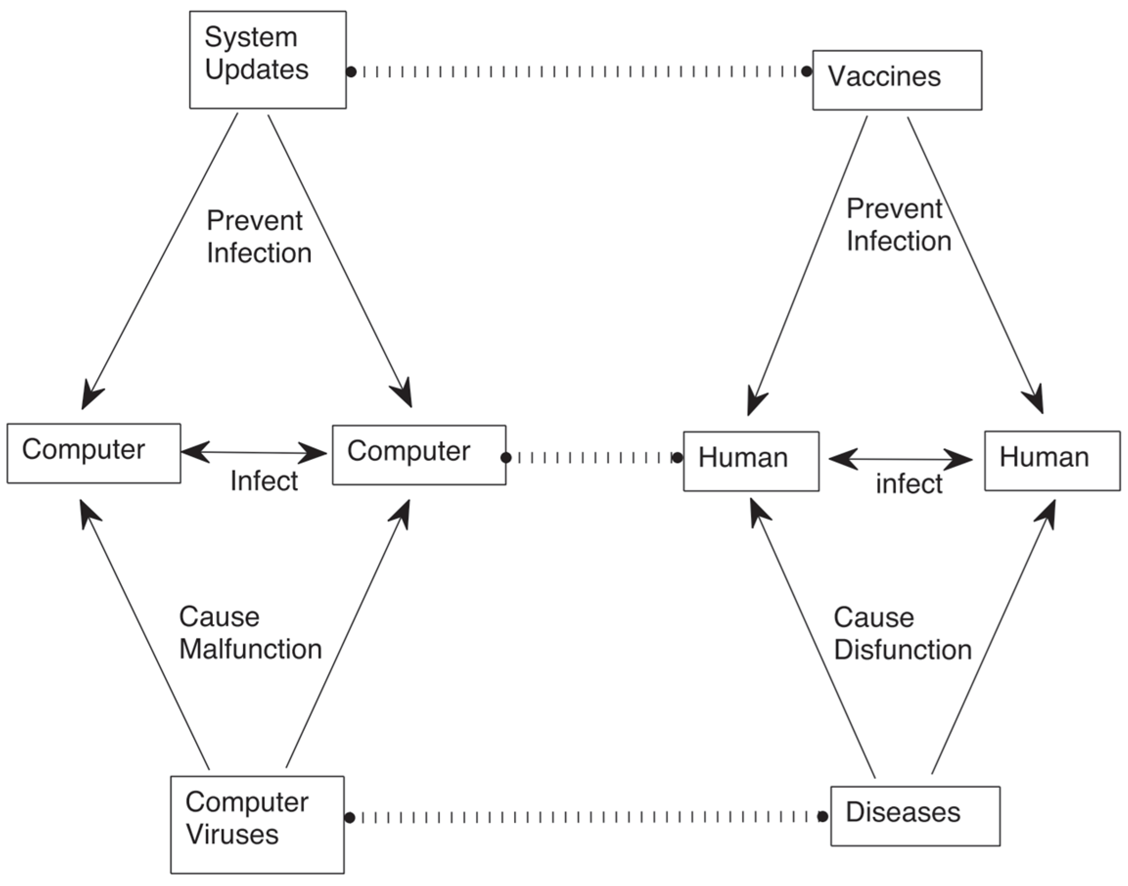
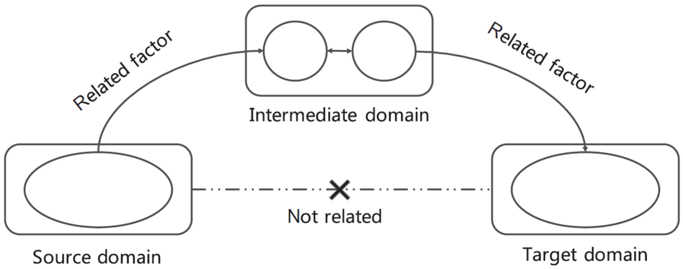
1.3. The Potential of Cross-System Transfer Learning

The discussion of cross-system transfer learning is particularly meaningful and important in the field of aerospace. Compared to other machines, aeroplanes are expensive assets that consist of complex systems with numerous components, which brings a unique challenge when trying to obtain the large amount of fault data required to develop fault diagnosis algorithms. To overcome this challenge, a common procedure to acquire fault data for aircraft systems is to design lab-based experiments or computational simulations based on the target systems, such as the three studies outlined in the following. The first system is the environmental control system (ECS). Designed by Jennions et al. [15], a simulation platform for ECS was created with components built through governing engineering equations. The simulation results were validated against the Boeing dataset to ensure it produced reliable, healthy cases. Then, faults were injected into the simulation to collect various fault data based on physics. The second system is the Auxiliary Power Unit (APU). Skliros et al. [16] ran experiments on a real APU for Boeing 747-400 to collect a validating dataset for the APU simulation platform, where a variety of fault modes can be simulated and studied. The third system is the aircraft’s fuel system. Since the actual fuel system on commercial aircraft is too complicated, a benchtop test rig was constructed to include only a simple fuel feeding loop. By injecting various faults into the test rig, fault data were collected. Using this test dataset as a baseline, Li et al. [17] constructed a simulation platform that enabled complex fault modes to be injected and collected. Each dataset of the three systems was the result of years of work, as all steps described above are necessary to derive a reliable simulation that can generate enough fault data to train a fault diagnosis model. Therefore, there is a need for more efficient fault diagnosis solutions, and applying TL to transfer diagnostic knowledge between each of the three systems above could be a solution. Upon the successful application of cross-system TL, the workload described above could be partially relieved because less training data are required for an equally accurate diagnosis.

In summary, the application of cross-system TL is a novel way to solve the challenges of fault diagnosis in a data-lacking situation, which bears the potential to improve the efficiency of CBM.

2. Datasets

This section presents the details of the three aircraft systems of interest. Section 2.1, Section 2.2 and Section 2.3 introduce ESC, APU, and the fuel system studied in this work by describing their working principles and key parameters. Section 2.4 summarises and compares the key features of the datasets associated with the three systems.

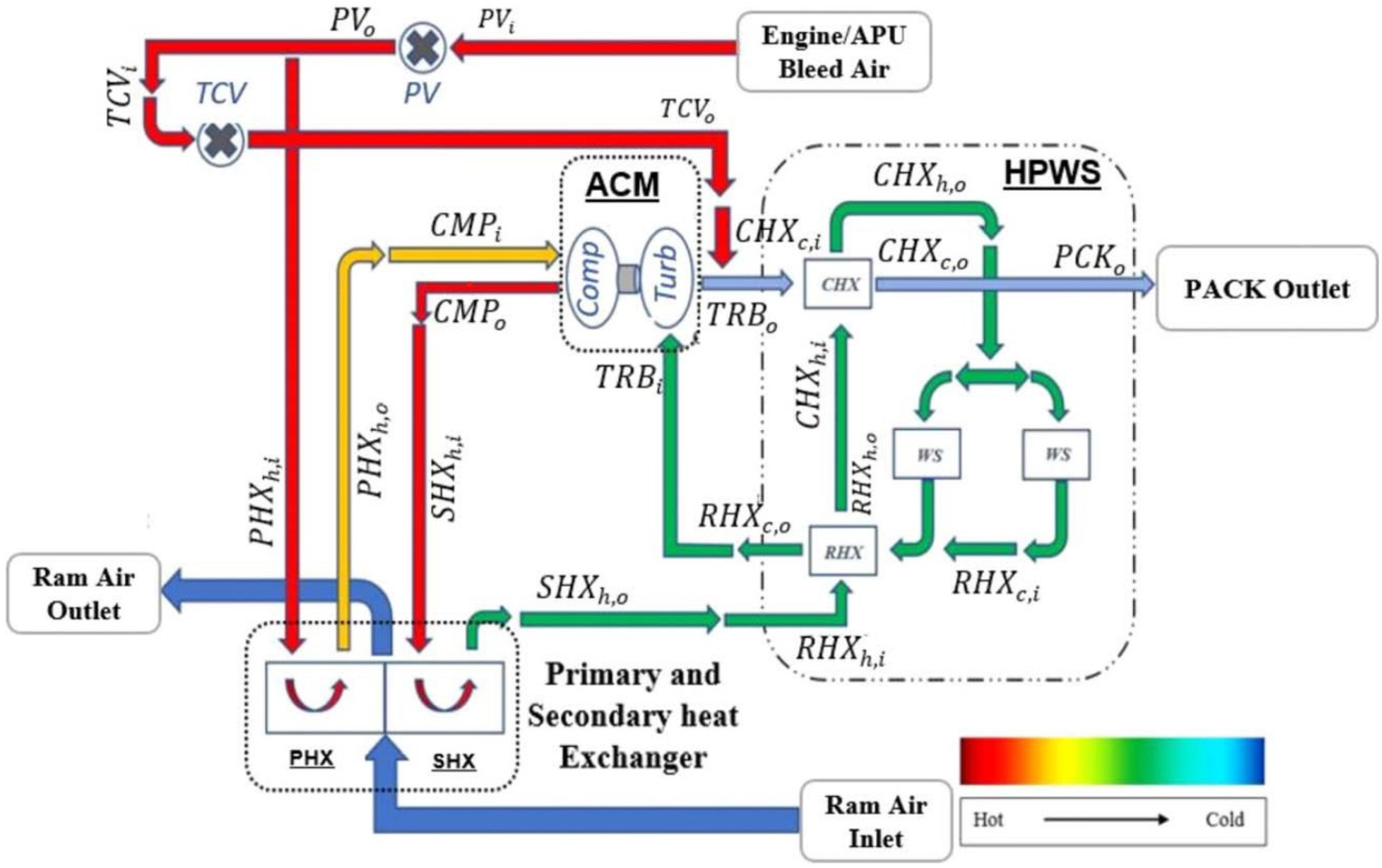
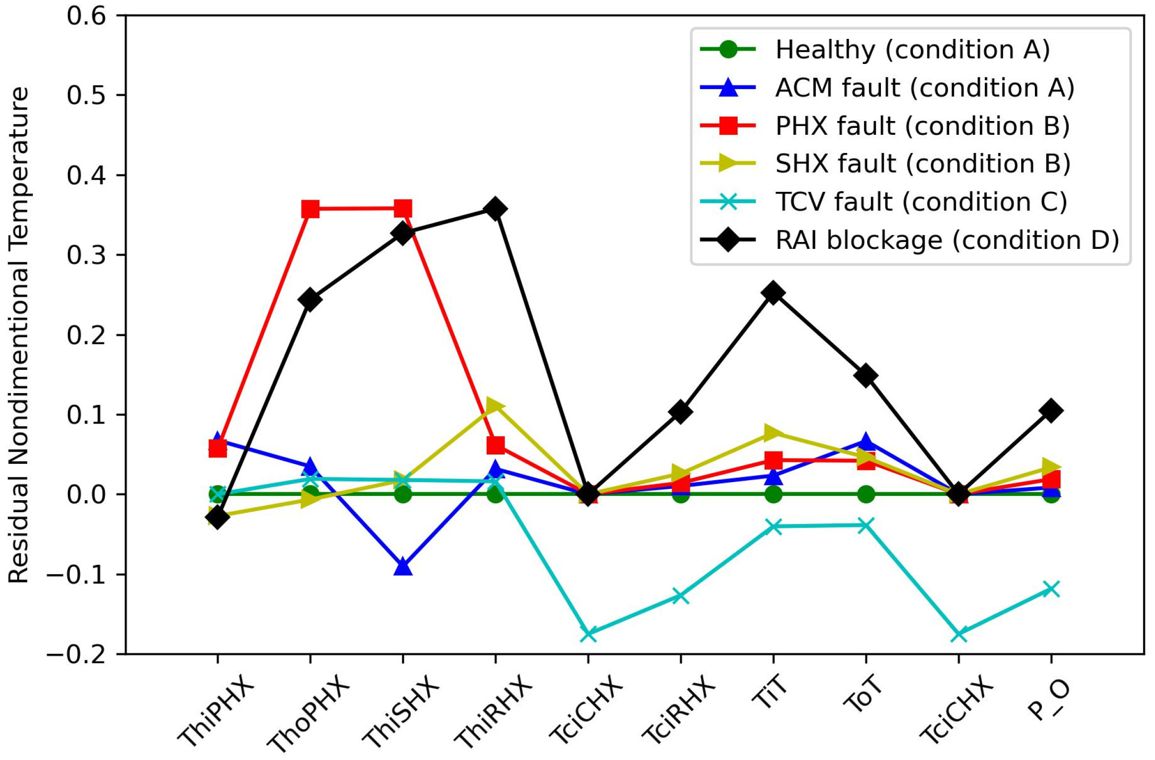
2.1. ECS Description

The ECS is an important aircraft system that supplies conditioned air for cabin pressurisation and equipment cooling [15]. For the Boeing 737-800, the essential subsystem within the ECS that conditions the engine’s bleed air is called the Passenger Air Conditioner (PACK) [18], a schematic of which is shown in Figure 1. Hot bleed air is drawn from the engine compressor at a flow rate commanded by the PACK valve (PV). A proportion of it goes through the temperature control valve (TCV), which mixes with the rest of the bleed air that has been cooled. Ram air serves as the heat sink for the cooling process at the two heat exchangers: the primary heat exchanger (PHX) and the secondary heat exchanger (SHX) [18]. The compressor in the air cycle machine (ACM) raises the pressure and temperature of the air after it passes through the PHX to improve the effectiveness of SHX [15]. A high-pressure water separator (HPWS) regulates the humidity before the air reaches the PACK outlet [18].

Data have been collected for the B737-800 PACK from a validated simulation platform, SESAC (Simscape ECS Simulation under All Conditions) [15]. The simulation of PACK was conducted at four different operating conditions, including three cruising conditions and one ground-running condition, all based on real flight data. The temperature profile was taken for each case and was determined to be adequate for fault classification. Each temperature profile is first normalised by the corresponding target temperature, and then the deviation from its respective healthy baseline case is taken to produce the input data as a residual. A plot of representative cases for the ECS is shown in Figure 2, with parameters aligned with the locations shown in Figure 1. Five single-fault mode cases and one healthy case are shown in Figure 2. It is clear that each different fault mode exhibits a distinct fault pattern. More details regarding the ECS dataset can be found in [18,19].

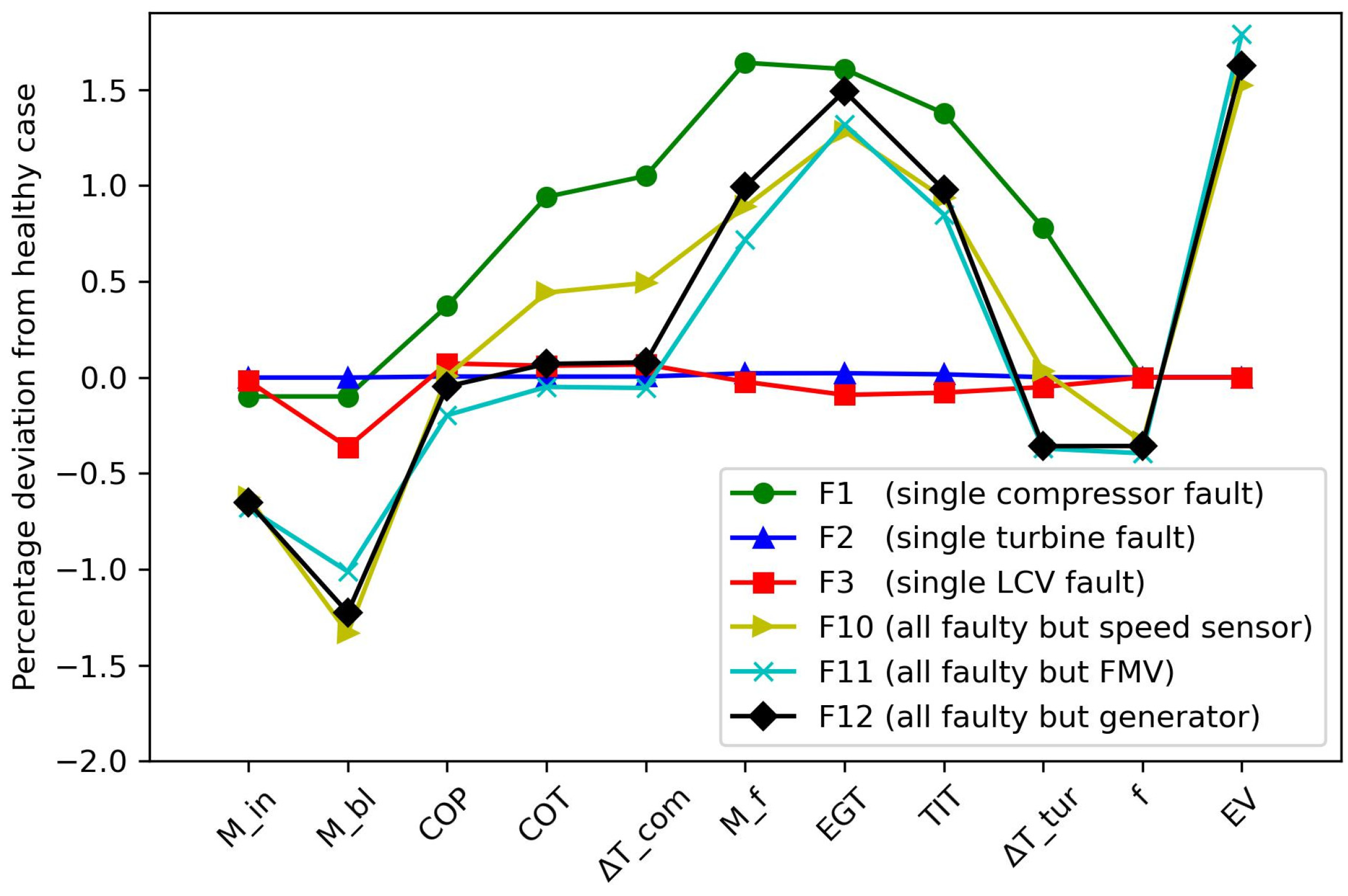
2.2. APU Description

The APU, a gas turbine-powered device located in the tail of a commercial aircraft, has the function of providing bleed air and electrical power to aircraft systems during the time before engine start-up on the ground or during the time of an emergency in flight [20]. The schematic of a Boeing 747 APU is plotted in Figure 3. The left part of the schematic shows a single-spool gas turbine engine comprising a compressor, burner, and turbine. To maintain constant rotational speed at all loads and conditions, an electronic turbine controller (ETC) in a feedback control loop with speed sensor feedback is imposed on the fuel metering valve (FMV) that controls the fuel flow into the burner [20]. Bleed air is drawn from the APU compressor via a load control valve (LCV). The gas turbine is connected to a generator through a gearbox. To maintain constant voltage output regardless of the load, rotational speed, and generator health, an automatic voltage regulator (AVR) is used to adjust the excitation voltage (EV) [20].

The dataset for APU is generated from a data-driven simulation platform and validated against experimental data from a real APU [16,20]. The parameters monitored are shown in the output section in Figure 3. Multiple fault modes are considered for the APU, with details summarised in

Table 1. Summary of the three datasets used in this paper.

	ECS [19]	APU [20]	Fuel System [17]
Number and nature of parameters	10 temperatures	3 mass flow rates, 5 temperatures, 1 pressure, 2 electric signals, 1 frequency	7 pressures, 3 volumetric flow rates
Operating condition	Ground running (Condition A), 28k ft cruise (Condition B), 35k ft cruise (Condition C), 41k ft cruise (Condition D)	Single condition	Single condition
Number of cases collected	288	300	3989
Components where fault is inserted (failure modes)	ACM (Fouling/blockage) PHX (Fouling/blockage) SHX (Fouling/blockage) TCV (Deviation from commanded position) RAI door (Blockage)	Compressor (Reduced efficiency) Turbine (Reduced efficiency) LCV (Deviation from commanded position) Speed sensor (Positive bias) FMV (Sticking valve) Generator (Increased stator resistance)	Boost pump (External leakage—failure a) Boost pump (Internal leakage—failure b) FOHE (Clogging—failure c) FOHE (Leakage—failure d) Nozzle (Clogging—failure e)
Health states considered	1 healthy state	F1-F6: single fault of each component	1 Healthy state
	5 single fault states for each component	F7-F11: one component healthy, all others faulty	F1-F5: 1 component faulty, all others healthy
		F12: all components faulty	F6-F15: 2 components faulty, all others healthy
			F16-F25: 3 components faulty, all others healthy
			F26-F30: 4 components faulty, one healthy
			F31: all 5 components faulty

. Since the parameters are of a different nature, APU data are processed into a percentage derived from a corresponding healthy case, and representative cases are drawn in Figure 4. Among the cases plotted, the three multiple fault cases are clearly less distinguishable from one another compared to the single fault cases. Therefore, it is apparent that the complex fault patterns brought by the mixture of degradation of multiple components could pose a challenge for intelligent fault diagnosis (IFD) algorithms. More details on the simulation and fault modes can be found in [16,20].

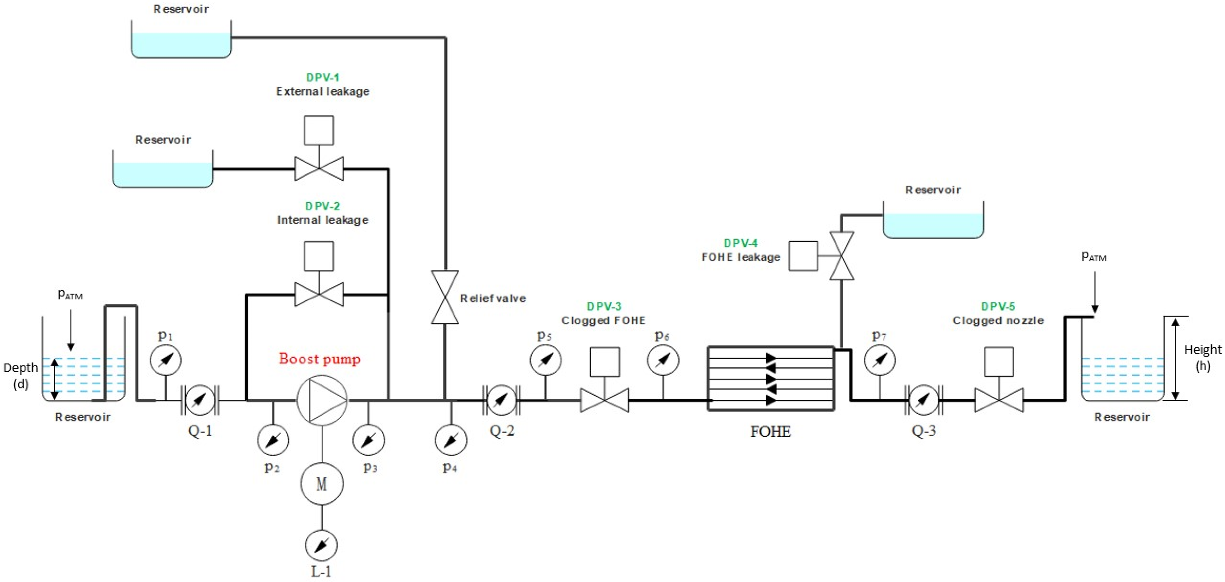
2.3. Fuel System Description

The fuel system studied is based on a benchtop water-based test rig, which has been wired up to include all major components of an aircraft fuel system [17], such as the reservoir, pump, and fuel–oil heat exchanger (FOHE). Using experimental data, a fuel system simulation was built in ref. [17], and its schematic is shown in Figure 5. Fuel is drawn from the reservoir on the left by a boost pump and then travels through the FOHE before reaching the reservoir on the right. Additional valves are added to the system to simulate leakages and clogging along the system, which are also plotted in Figure 5.

The dataset for the fuel system is derived from simulations of all possible health conditions of the system, which is summarised in Table 1. The pressures are recorded in bars, and the volumetric flow rates are in millilitres per second. Each case is then taken from the deviation of the healthy baseline and represented as residual data. Six representative cases are plotted in Figure 6. Considering a wide array of multiple faults, fuel system data also contain cases that are hard to distinguish, such as the F16 and F26 cases in Figure 6. More details regarding the simulation can be found in [17].

2.4. Dataset Comparison

The key features of the three systems, the ECS, APU and fuel system, are summarised in Table 1. Since the three systems are fundamentally different, their parameters and fault modes show no similarity, which is evident from the representative plots for the three datasets shown in Figure 2, Figure 4 and Figure 6. In addition, because the three datasets were generated under different research projects and backgrounds, the operating conditions and fault simulation levels were not consistent, which added to the complication of knowledge transfer between them. In summary, the distinct comparison between the three datasets signifies that any knowledge transfer across the systems takes place between very distant domains and makes the discussion of possible ways to transfer diagnostic knowledge between the three systems reasonably realistic.

3. Methodology

The methodology of this work is summarised in Figure 7. To explain the methodology with clarity, Section 3.1 describes the exact real-world challenges in IFD that this work attempts to address and how the three datasets are used in each domain of transfer to reflect such challenges. Section 3.2 and Section 3.3 outline two possible approaches to address the problem raised in Section 3.1. Section 3.2 presents a TL solution based on 1D-CNN, where the analogy between features is exploited to achieve cross-system knowledge transfer. Section 3.3 describes another TL solution based on 2D-CNN, where IFD in both the source and target domains are treated as image classification problems to enable cross-system transfer.

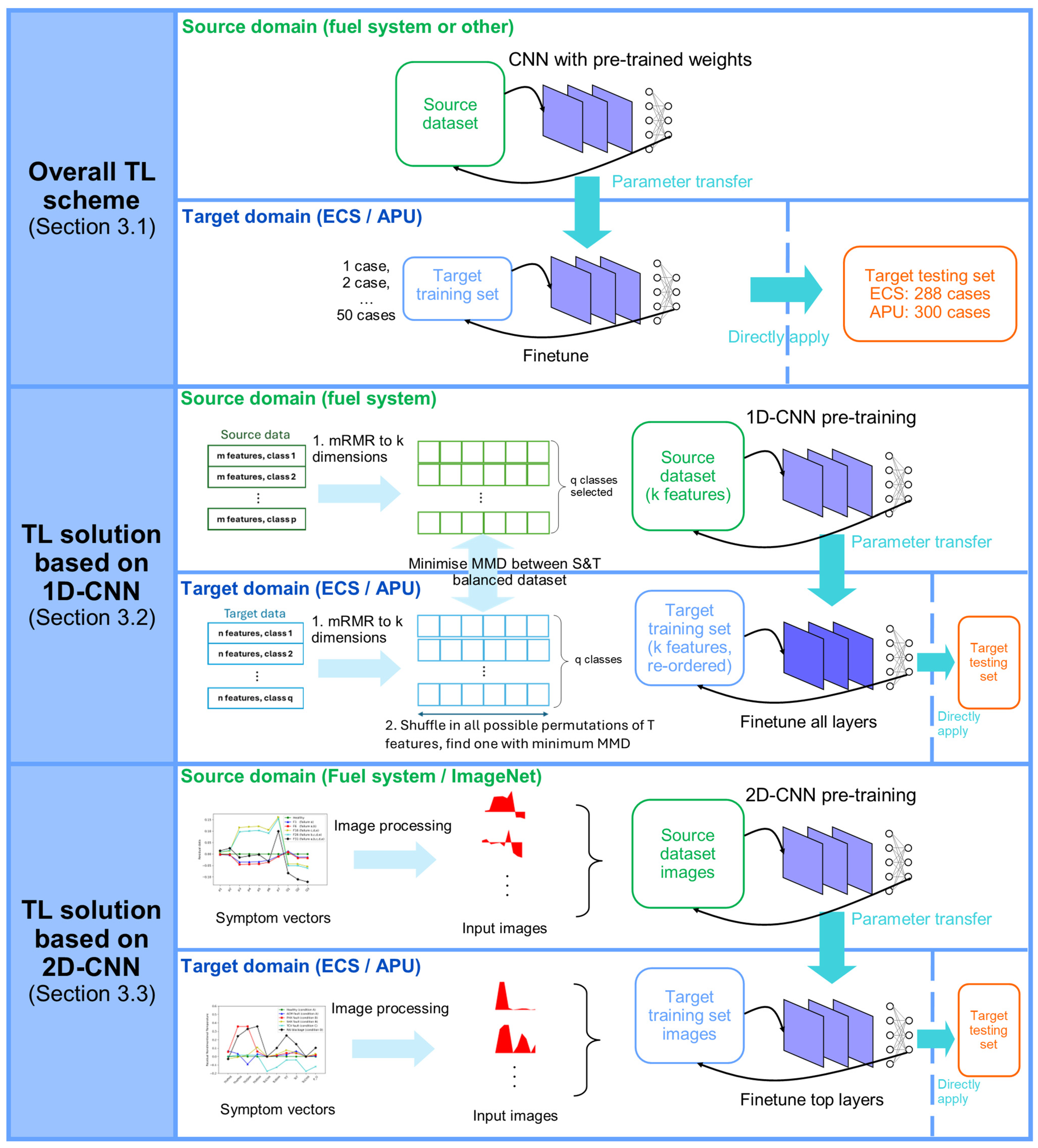
3.1. Transfer Learning Problem

The three systems, the ECS, APU and fuel system, are all accompanied by validated simulation platforms that are capable of generating reliable data under a variety of conditions and degradations. These simulations have enabled the collection of the three datasets summarised in Section 2.4 with the possibility of generating further data if required. In addition, the data generated are well labelled and balanced to facilitate the training of IFD algorithms. However, such simulations are not always possible to derive or economical to implement, which poses challenges to real-world IFD. Hence, this work seeks to explore scenarios that more closely resemble real-world engineering systems as a small sample problem where a well-populated, labelled, balanced dataset is not available. In terms of TL domains, the real-world challenge is that there is only a small, labelled dataset available for training in the target domain. In practical terms, after receiving a large quantity of data from a machine, an engineer with expert knowledge would need to manually label the cases, which gives rise to the labelled dataset that can then be used to train an IFD algorithm for the machine. Due to the cost of labelling and difficulty in gathering abundant faulty cases, this labelled training dataset is generally small in real-world applications, hence the assumption in this work.

The selection of datasets in the source and target domains can be arbitrary, but working with the three datasets available, the natural choice would be to select the fuel system as the source domain since it is a much richer dataset than ECS and APU in terms of the number of cases and health states. Therefore, this work uses the ECS and APU datasets in the target domain, and the real-world IFD challenge is simulated by only assuming that a small subset of the ECS and APU datasets is available for training. Figure 7 illustrates the setting of the problem and datasets in the source and target domains. As the later sections will show, the deep learning method based on the convolutional neural network (CNN) performs better than traditional machine learning (ML) methods; as such, the TL solution is based on CNNs. Thus, the overall TL process would be first transferring a CNN pre-trained by fuel system data or other data. Then, a small subset of the target domain dataset, i.e., 1-to-50 labelled cases from ECS or APU, is used to finetune the transferred CNN for target domain problems. Each run with 1 to 50 training cases in the target domain can simulate a case in reality where very limited training data are acquired for a system. Finally, to evaluate the accuracy of the finetuned CNN, it is directly applied to the entire ECS or APU dataset to reflect how the TL-based IFD solution would perform in predicting the system’s health condition after implementation.

In addition to a small, labelled training set, there are other features of the ECS and APU datasets that add to the challenge for IFD solutions. Regarding ECS, since data are collected from four operating conditions, the 1-to-50 case training set contains a random mix of cases with different conditions. As a result, the distribution of the discrepancy of cases with different conditions and the possibility of encountering unseen conditions in the testing set could add a challenge to IFD solutions. As for APU, half of the dataset involves multiple faults, so the complex fault patterns result in confusion between classes and raise the difficulty of training accurate IFD solutions.

3.2. Transfer Learning Solution Based on 1D-CNN

Since each case in the three datasets is represented by a 1D symptom vector, the natural choice of the IFD algorithm is a 1D CNN or ML classifier. As later sections will show, 1D-CNN outperforms other traditional ML classifiers when solving the problem without TL, so taking 1D-CNN forward to develop a TL solution between different systems is a viable first attempt. However, within the field of IFD, no TL work between distant domains using 1D-CNN has been found; hence, a novel TL method based on 1D-CNN is required to leverage knowledge from the fuel system to ECS or APU.

To derive such a method, a branch of TL that is rarely used in engineering applications is considered for its ability to transfer knowledge between seemingly unrelated domains; this is called relation-based TL. For distant source and target domains, relational TL focuses on the structure or relations between data instances and transfers knowledge based on high-level structural commonality in the two domains, thereby bypassing the lack of low-level data similarity between distant domains [6]. A specific approach to relation-based TL that is most relevant to the problem of interest is transfer learning by structural analogy. This method is inspired by how humans are able to make an analogy across different domains and learn in seemingly irrelevant domains via structural similarities [6]. An example of such a high-level structural similarity is shown in Figure 8. Despite the fact that computer viruses and human diseases appear unconnected, humans infect one another with diseases in a comparable manner as computers infect one another with viruses, which can be seen as a structural similarity. Using transfer learning by structural analogy [13] has helped demonstrate how knowledge in diagnosing cardiovascular diseases helps improve the accuracy of diagnosing respiratory tract diseases.

Diagnosing disease in the different human systems mentioned above is a similar task to diagnosing the health status of different aircraft systems; the design principle of transfer learning by structural analogy served as a guideline for designing the 1D-CNN TL solution to transfer knowledge from fuel system data to ECS and APU. In the disease diagnosis example in [13], the ultimate goal of transfer learning by structural analogy is finding analogical pairs of words in the two domains of diseases. Then, by treating the words in the analogical pairs from the two domains as equivalents, a diagnosis algorithm trained in one domain can be transferred to another domain to improve diagnostic accuracy. Optimisation in finding the best analogical pairs is achieved by maximising two goals simultaneously: (1) selecting features that are most relevant to label prediction in the source and target domain, respectively, and (2) finding pairs of analogical features to produce maximum structural similarity between the source and target domain [13].

Because data instances from the fuel system, ECS, and APU are clearly different numerically, finding similar patterns in each data instance between the fuel system in the source domain and ECS and APU in the target domain is crucial, which is a similar idea to relation-based TL. To enhance the possibility of finding similar patterns in the source and target data instances, aligning the order of the source and target domain features according to the analogical pairs is a promising approach. For the problem of interest, the two goals of finding the analogical pairs of the source and target domain features in transfer learning by structural analogy are still followed, but they are achieved in two separate steps: (1) the label dependency of the features is calculated by minimum redundancy maximum relevance (mRMR), which selects the most important features in both the source and target domains while reducing the source and target domain data to the same dimension; (2) the structural similarity between the source and target domain is maximised by finding the order of target domain features that produce the minimum MMD (maximum mean discrepancy) distance between the two datasets. At the end of the process, both the source and target domain datasets have the same dimension, with features reordered according to the analogical pairs. Therefore, a 1D-CNN pre-trained with the fuel system dataset can be transferred to the target domain, where the ECS or APU training set can finetune the transferred CNN before testing on the whole dataset. This entire process is captured in Figure 7.

3.3. Transfer Learning Solution Based on 2D-CNN

3.3.1. From Image Classification to Fault Diagnosis

Another approach to achieving cross-system TL is based on 2D-CNN. This is a common approach found in IFD applications, such as [21,22,23], which essentially exploit the pre-trained 2D-CNN, using the ImageNet dataset, to improve the fault diagnosis accuracy. Despite the fact that there is no relevance between the images in ImageNet and the signal images for IFD, since 2D-CNN treats the IFD problem in the same way as image classification, knowledge can be transferred from a very distant source domain such as ImageNet. Not limited to using ImageNet as the source dataset, Liu et al. [24] transferred 2D-CNN between two different chemical processes and reported improvement in diagnosis accuracy as a result. Therefore, using image classification as the media, TL based on 2D-CNN is capable of transferring knowledge between distant domains that can be represented by images. This approach can be considered transitive transfer learning (TTL), a branch of TL that transfers knowledge through one or more intermediate domains, bridging the large gaps between the source and target domain [6]. The general idea of TTL is shown in Figure 9. For distant domains, such as the fuel system and ECS or APU, the common factor is that both systems have fault patterns, which can be represented graphically. Thus, the intermediate domain can be achieved through image classification, where 2D-CNN can be transferred from the fuel system to the ECS or APU. In summary, a cross-system TL solution based on 2D-CNN is a justified approach for the problem based on existing IFD applications and the TTL framework.

The process of implementing a cross-system TL solution based on 2D-CNN is illustrated in Figure 7. Each case in the dataset is converted from symptom vectors to input images into 2D-CNN. Both the fuel system dataset and ImageNet dataset are considered the source domain, and a comparison was made between them to determine which source domain performed better for the problem. The pre-trained CNN from the source domain was transferred to the target domain, where the small ECS or APU training set was used to finetune the top layers before testing on the whole dataset. Several popular deep networks were tested initially, and the best-performing model, ResNet101, was chosen as the base model for the 2D-CNN. Top layers with customised output label spaces were added to the base model to fit the different number of classes in the three systems, as shown in

Table 2. Details of the ML classifiers and deep models used.

ML Classifiers	Key Parameters
kNN	n_neighbors = 3
SVM	kernel = ‘linear’, decision_function_shape = ‘ovo’
DT	max_depth = 4, criterion = ‘entropy’
RF	n_estimators = 30, max_depth = 4, criterion = ‘entropy’
Deep networks	Information of layers
1D-CNN	Input layer Conv1D layer (filters = 16, kernel_size = 4, padding = ‘causal’) Conv1D layer (filters = 32, kernel_size = 6, padding = ‘causal’) Conv1D layer (filters = 64, kernel_size = 8, padding = ‘causal’) MaxPooling1D layer Flatten layer Dense layer (units = no. classes, activation = ‘softmax’)
2D-CNN	Base model: ResNet101 from Keras Applications, pooling = ‘max’ Top layers: Flatten layer Dense layer (units = 256, activation = ‘relu’) Dense layer (units = no. classes for the target systems, activation = ‘softmax’)

.

It is worth noting that while the TL solution based on 2D-CNN enables cross-system transfer from the fuel system to ECS and APU, an additional benefit it brings is the possibility of using ImageNet as the source domain. Since ImageNet is an incredibly rich dataset with over 14 million images [25], using the pre-training weight from ImageNet provides a highly accurate and reliable CNN. The existence of established weights for most common CNN models also saves on pre-training computational costs. In this work, the ResNet101 model with ImageNet pre-training weight was taken from He et al. [26].

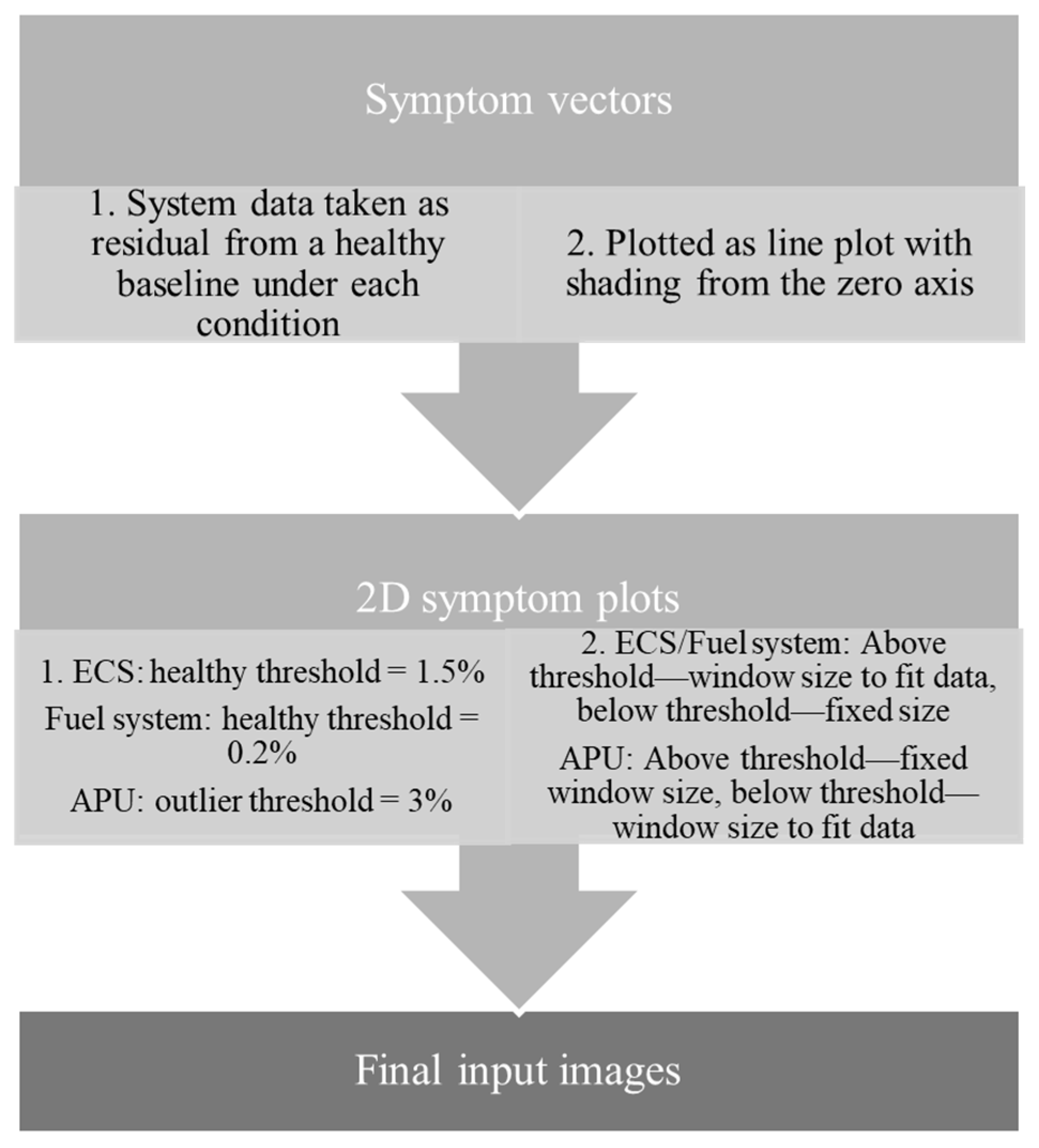
3.3.2. Image Preparation

To feed the data from the three systems into 2D-CNN, data instances need to be converted into images. Figure 10 illustrates the workflow needed to prepare the input images for the 2D-CNN. Starting from the symptom vectors of residual data, each case is first plotted as a line plot, and the area between the line and the horizontal zero axis is shaded to aid image recognition. On top of that, the choice of window size is carefully selected. In the ECS case, a threshold of 1.5% deviation from the healthy baseline is chosen. Any data instances below the threshold are considered healthy; hence, a fixed window size is applied to the final input images to avoid zooming into the minute deviations and causing misclassification. The data instances above are likely to be faulty cases; hence, a flexible zoom is allowed to fit the maximum and minimum in the image, which helps to amplify the fault signature. In the APU, due to a lack of consideration of healthy cases, the window size is determined with the aim of reducing the influence of an outlier parameter, ETC_S, which reaches a 100% negative in some cases where there is complete signal loss. An outlier threshold of 3% deviation from the healthy baseline is set so that any data exceeding this limit will have a fixed window size to focus on the parameters other than the outliner signal. The final input images are fed into 2D-CNN without an axis and labels, such as the ones shown in Figure 7, to allow the model to focus on fault patterns.

4. Results and Analysis

This section shows the results of the solutions for the problem of interest. To verify if the two cross-system TL approaches for the problem are meaningful, Section 4.1 first establishes the baseline result followed by a non-TL approach. Common ML classifiers and a 1D-CNN were applied to the small sample problem in ECS and APU, and a 1D-CNN was found to produce the best result. Thus, the 1D-CNN result without TL will be used as a uniform baseline to verify if the TL result in Section 4.2 shows a positive transfer. Section 4.2.1 shows the result after applying the TL solution based on 1D-CNN using the fuel system as the source domain. The result from the 1D-CNN-based TL solution shows limited improvement from the baseline result. Finally, Section 4.2.2 shows the result following the 2D-CNN-based TL solution, where an improvement was found for both ECS and APU problems. All predictive accuracies in this paper refer to the standard multiclass classification accuracy calculated by the ratio of correct classifications out of all the classifications.

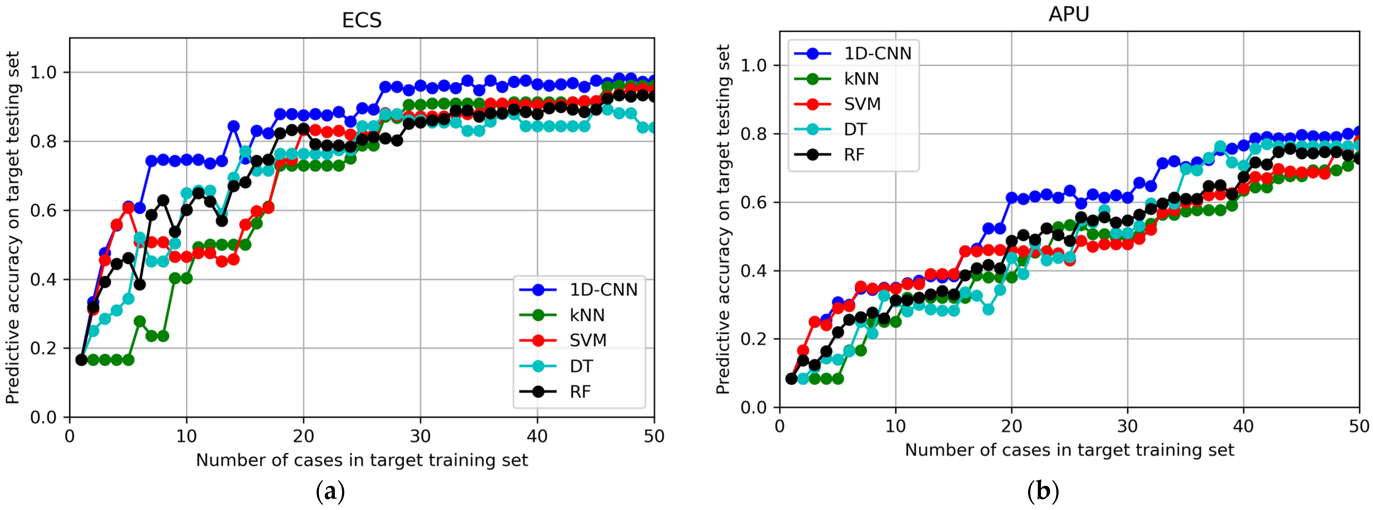
4.1. Baseline Result from Non-TL Methods

To understand how the conventional ML algorithm performs for the small sample problem in both ECS and APU datasets, a variety of common ML classifiers were selected, and a 1D-CNN model was constructed. The classifiers used included k-nearest neighbours (kNN), support vector machine (SVM), decision tree (DT), and random forest (RF) [27], which represent the most commonly used classifiers in existing IFD applications. The key parameters of the ML classifiers used in this work are listed in Table 2. The architecture of the 1D-CNN is also shown in Table 2. This was constructed using the Keras library [28]; the 1D-CNN model used contained three convolutional layers: a maximum pooling layer, a flattening layer and a dense layer. This 1D-CNN architecture was determined by a trail and error approach on the datasets used to generate the best accuracy and fastest convergence, and the parameters used in each layer are detailed in Table 2.

The results are shown in Figure 11 and summarised in

Table 3. Summary of average accuracy from non-TL methods.

Method (Non-TL)	Average Predictive Accuracy (%) for Testing Set
	1–30 Cases in ECS Training Set	1–50 Cases in APU Training Set
1D-CNN	76.48	56.92
kNN	54.36	44.81
SVM	63.16	48.96
DT	64.21	48.24
RF	65.96	49.25

. Figure 11 plots the predictive accuracy for the entire ECS and APU datasets against the number of cases in the training set ranging from 1 to 50. From Figure 11, the ECS results from most methods rarely show any meaningful change when 30 or more cases are in the training set, so analysing the scenario where 1 to 30 cases are in the training set would make a comparison between the methods more obvious. However, the results from most methods when dealing with the APU dataset showed a continuing trend when cases in the training set increased from 1 to 50, so the entire range will be considered.

Hence, the average predictive accuracy for the testing set was calculated for each method when 1 to 30 cases were used in the ECS training set, and 1 to 50 cases were used in the APU training set, which is shown in Table 3. Although, in reality, a small sample problem would be one single scenario with a certain small number of cases in the training set (e.g., 20 cases in the ECS training set when designing the ECS diagnosis algorithm), taking an average in the way described above is useful to summarise a range of possible small sample problems and compare different methods. Judging by this metric, 1D-CNN outperformed all other ML methods. For the ECS case, the 1D-CNN average accuracy was 76.48%, which is 10.52% higher than the second-best method, the RF classifier. For the APU case, the average accuracy of the 1D-CNN was 56.95%, which is 7.67% higher than the second-best method, the RF classifier. In addition, it can be observed from Figure 11 that the 1D-CNN result in each of the ECS and APU scenarios is consistently the best one among all the methods used. Therefore, the result from the 1D-CNN will be used as the baseline non-TL result, representing the best performance of conventional ML methods.

4.2. Result from TL Methods

Two TL approaches were implemented, and the results are shown in the sections below. The results from the 1D-CNN-based TL solution are shown in Section 4.2.1, and the results from the 2D-CNN-based TL solution are shown in Section 4.2.2. To determine whether the TL methods achieved positive transfer, all TL results were checked against the non-TL baseline from 1D-CNN.

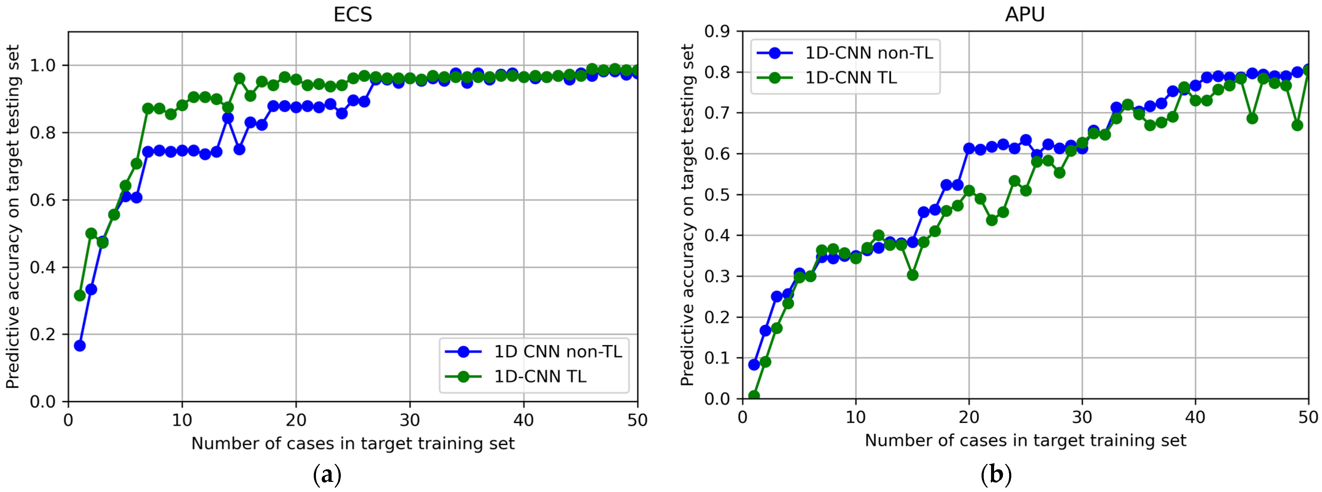
4.2.1. Results from TL Method Based on 1D-CNN

Figure 12 shows the accuracy of the 1D-CNN-based TL solution in the target domain testing set against the number of cases in the target domain training set for ECS and APU, using the fuel system as the source domain. The non-TL baseline result was plotted on the same graph for comparison. From Figure 12, it can be observed that the 1D-CNN-based TL solution significantly improves the accuracy in almost all 50 scenarios for the ECS compared to the non-TL baseline; yet, the same trend is not seen in APU. For the APU, the TL methods with 1D-CNN performed worse than the non-TL baseline in general.

For the same reason as described in Section 4.1, the average predictive accuracy for the target domain testing set was calculated for the first 30 scenarios for ECS and all 50 scenarios for APU. Regarding ECS, the average predictive accuracy following the TL solution with 1D-CNN was 84.98%, compared with non-TL baseline predictive accuracy of 76.48%. The significant improvement in ECS diagnostic accuracy with TL from the fuel system demonstrates the effectiveness of the 1D-CNN-based TL solution on this dataset. The positive transfer should be attributed to the ability of the TL method to transfer pattern recognition capacity from the fuel system dataset to the ECS dataset, which shows positive knowledge transfer across the two systems. In contrast, the average accuracy of the APU following the TL method was found to be 52.84%, which is 4.08% lower than the non-TL baseline. Hence, a negative transfer took place from the fuel system to APU.

The opposite behaviour of the TL solution based on 1D-CNN was to be expected, given the fact that the three systems discussed in this work were vastly different, which means finding similar patterns between them is not always guaranteed. In terms of the principle of the 1D-CNN-based TL solution, it would only work if there was an order of target domain features that produced similar patterns for certain classes of data compared to the source domain. However, for distinct systems, such an order may not exist, which could explain the result in APU. Additionally, the current method of rearranging target features may not be the optimal way to seek similar patterns in source and target domains, which is also a potential reason for the negative transfer case for APU. In summary, given the improvement in ECS and degradation in APU, the TL solution based on 1D-CNN can be concluded as effective under certain source and target domains but not for all combinations of source and target systems. Therefore, an alternative TL solution must be considered for the distant source and target domains of the ECS and APU problem, such as the TL solution based on 2D-CNN introduced in Section 3.3.

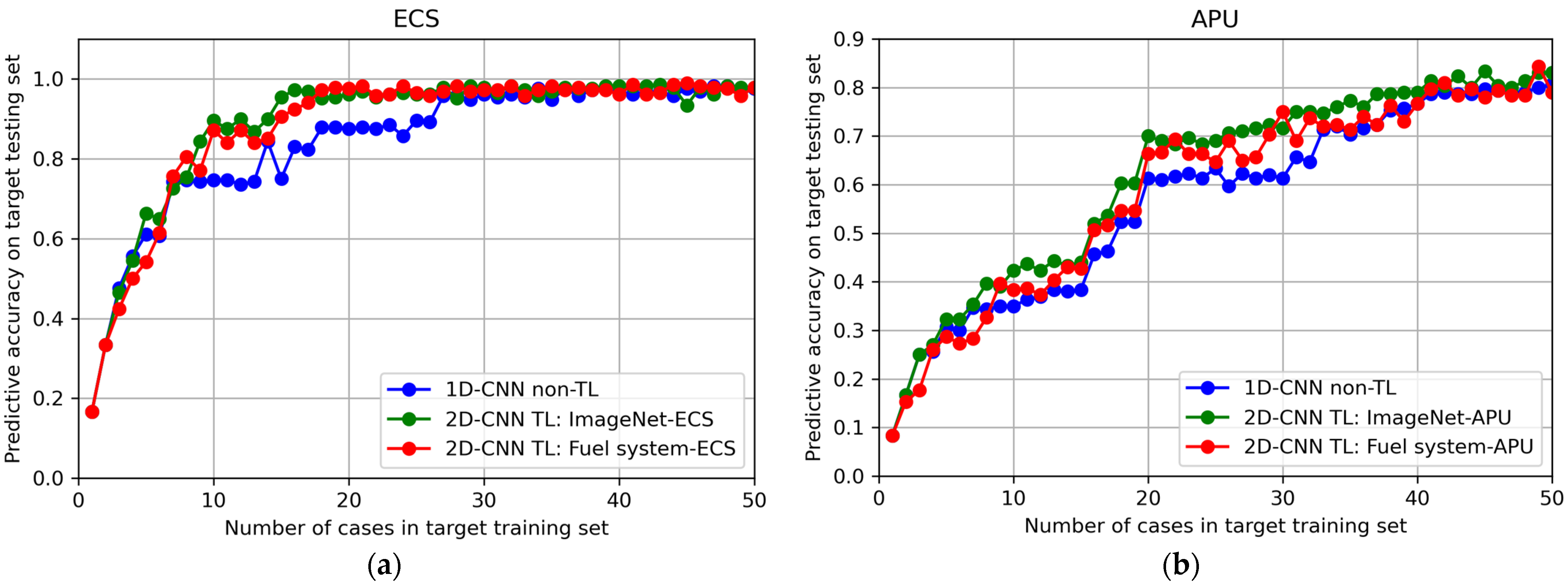
4.2.2. Results from TL Method Based on 2D-CNN

The results from the 2D-CNN-based TL solution are plotted in Figure 13, and key metrics are summarised in

Table 4. Summary of results of 2D-CNN TL solution.

Method	Average Predictive Accuracy (%) for Testing Set		Minimum Number of Cases in Training Set to Reach
	1–30 Cases in ECS Training Set	1–50 Cases in APU Training Set	95% Accuracy in ECS Testing Set	75% Accuracy in APU Testing Set
1D-CNN non-TL baseline	76.48	56.92	27	40
2D-CNN TL solution with ImageNet in source domain	83.38	61.96	15	34
2D-CNN TL solution with fuel system in source domain	81.96	58.95	18	40

. Two source domains, the fuel system and ImageNet, were used in this solution to pre-train the 2D-CNN, and the results following the TL process are plotted with the non-TL baseline. From Figure 13, for both ECS and APU, the 2D-CNN-based TL result from both source domains outperformed the non-TL baseline, demonstrating positive transfer. The average accuracy of ECS diagnosis when 30 or fewer cases existed in the target training set was 83.38% using ImageNet as the source domain, and the accuracy was 81.96% when using the fuel system as the source domain, corresponding to a 6.90% and 5.48% improvement, respectively. As for the APU, the average accuracies when there were 50 or fewer cases in the target training set were 61.96%, with ImageNet being the source domain and 58.95% with the fuel system as the source domain, resulting in a 5.04% and 2.03% improvement, respectively. It should be pointed out that the same 2D-CNN had been applied to the datasets in a non-TL setting, which resulted in extremely poor accuracy, so it is safe to rule out the concept that the improvement was brought about by the difference between the 1D-CNN and 2D-CNN. The results from non-TL 2D-CNN are not included as they do not have a significant contribution to the overall discussion.

Another useful metric to assess the performance of methods in the small sample scenarios in the target is also recorded in Table 4, which is the minimum number of cases each method requires to reach and stay above a certain level of predictive accuracy. This can assess how many cases are required by each method to produce an accuracy that is comparable to obtaining a large training set, i.e., the minimum number of cases needed in the training set to avoid the small sample problem. The smaller this number is, the more economical and convenient it is to apply the method in a similar real-world scenario. Using 95% as the accuracy in ECS and 75% as the accuracy in APU, the minimum number of cases required by each method is shown in Table 4. For the ECS, the 2D-CNN-based TL solution using ImageNet reduced the minimum number of cases to 15 compared to the 27 cases required by the non-TL method, which is a considerably smaller training set, hence justifying its superior capacity in real-world small sample challenges. The same trend is observed for the APU. The 2D-CNN-based TL using the fuel system as the source domain reduced the number of cases required in the ECS but not in the APU. In general, the 2D-CNN TL method is effective in increasing the accuracy obtained and reducing the minimum number of cases required to avoid the small sample problem.

5. Explanation and Evaluation of Results

Having determined that the 2D-CNN-based TL solution is effective in improving the predictive accuracy for both the ECS and the APU datasets when only small subsets of the dataset are available in the training set, Section 5 aims to explain the improvement in detail. Since the 2D-CNN tackles the IFD problem by recognising fault patterns in the input images, Section 5.1 introduces a visualisation method to find what fault patterns the network identifies, which can help validate the reason for positive transfer. From a different perspective, Section 5.2 discusses specific cases where the non-TL baseline method’s prediction falls short. By comparing the reasons behind why a non-TL method and a TL method produce different decisions, arguments to validate the knowledge transfer via 2D-CNN TL can be made. Finally, Section 5.3 discusses the behaviour of the TL solution based on 2D-CNN over complex fault patterns in APU multiple fault cases.

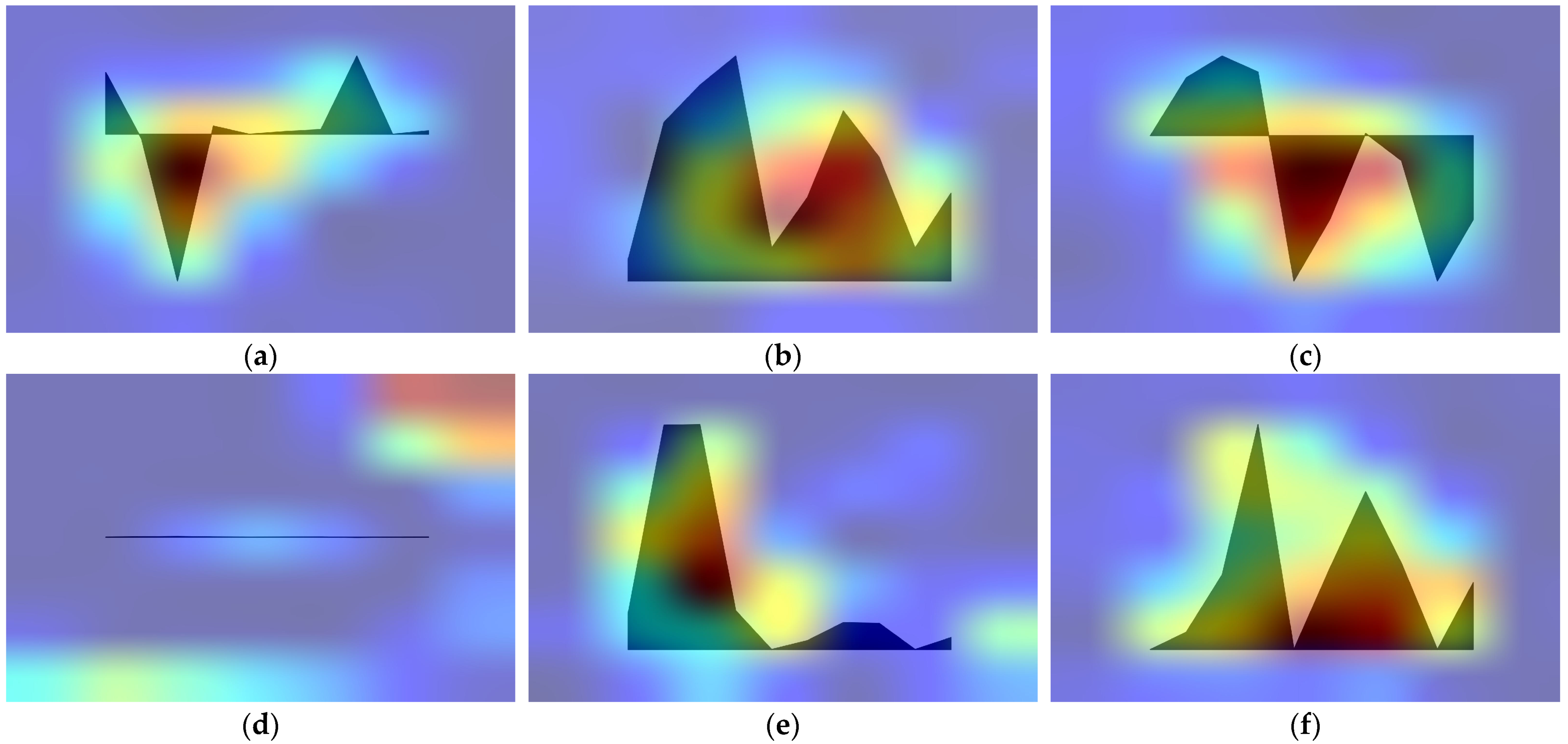
5.1. Grad-CAM Visualisation for 2D-CNN TL Result

To understand how deep networks make decisions about classification, a useful visual explanation tool, the Gradient-Weighted Class Activation Mapping (Grad-CAM) [29], is used. Using the gradient information that flows into the last convolution layer of a CNN model, grad-CAM assigns a value of importance to each neuron for a given decision, thereby localising the regions in the input image that contribute most to the decision [29,30]. Grad-CAM has been widely applied to address the ‘black box’ problem of deep models, and its success has also been seen in IFD applications [30]. Compared to other visual explanation tools, Grad-CAM is considered the state-of-the-art method that is applicable to any CNN without changing the CNN or requiring re-training [29].

Given a CNN model and input image, Grad-CAM generates a heatmap showing the concentration regions in the input image, which is useful to determine the fault patterns that the 2D-CNN-based TL solution has identified. In the scenario where only 15 cases were available for the ECS training set, the 2D-CNN-based TL solution generated the most significant improvement from the non-TL baseline. In this scenario, the 2D-CNN TL solution with ImageNet and fuel system data as the source gave 95.49% and 90.63% accuracy compared to 75.00% from the non-TL baseline. Therefore, this scenario has been selected to apply Grad-CAM to discover the reason for the improvement of the 2D-CNN TL solution.

Using the ImageNet dataset to train the network in the source domain, the 2D-CNN transferred to ECS diagnosis was analysed by Grad-CAM. A case with six ESC-degraded modes was taken, and their Grad-CAM heatmap for the transferred 2D-CNN is plotted in Figure 14a–f. Here, red represents the most important regions, and blue represents the least important regions. Figure 14 shows that the transferred 2D-CNN focuses on the major fault patterns in all fault modes. The only exception is Figure 14d, which shows the healthy case. Since the ECS data are processed to be residual data from the healthy baseline, the input image of a healthy case is basically a horizontal line in a blank background, so the Grad-CAM heatmap also shows a concentration in the blank background, given that the blank background might be a more significant feature to catch instead of the thin line. Nonetheless, the identification of a largely blank background is effective enough to identify a healthy case. In summary, since the concentration regions for each health mode are different and coincide with the major distinguishing features of the input image, it can be concluded that the transferred 2D-CNN identified the fault patterns of each mode, which is the basis for its accurate diagnosis performance.

Considering that the source domain, ImageNet, is an image dataset consisting of everyday items like pets, cars, fruits, etc., the target domain ECS datasets are composed of completely dissimilar pictures. However, since the ImageNet dataset contains over 14 million images in 1000 classes, the vast number of features that the pre-trained 2D-CNN can identify enabled the knowledge transfer to identify the ECS fault patterns in the target domain despite the content of the images in the source and target domains being unrelated. In comparison, the other choice of source domain, the fuel system data images, is a more similar set of images. However, since the fuel system dataset is much smaller than ImageNet, containing only 3989 images in 32 classes, there was a more limited pattern recognition capacity transferred to the ECS problem, hence the slightly worse performance of the 2D-CNN-based TL solution using the fuel system as the source. Nonetheless, the transfer from the fuel system to ECS and APU improved the accuracy, demonstrating the successful cross-system transfer ability of this method.

Although the cross-system TL solution underperforms the TL solution based on ImageNet for the three datasets used in this work, it is still a remarkable achievement that is worth further discussing in the future for two reasons. Firstly, it is more sensible from an engineering perspective to leverage diagnostic knowledge from one system to another. Using both engineering systems in the source and target domain, any physical similarity between them would lead to similar fault patterns and, hence, better diagnostic knowledge transfer based on their physics. The three systems used in this work were an extreme demonstration of completely different systems set up to fully test the feasibility of the cross-system TL methods. However, for systems resembling higher physical similarity, there may be more similar patterns between their faults that would promise higher cross-system TL accuracy. Secondly, despite the fuel system dataset being orders of magnitude smaller than ImageNet, the cross-system TL solution achieved a comparable level of improvement as the TL solution was based on ImageNet, which indicated a higher efficiency of diagnostic knowledge transfer. If another aircraft system was found to produce richer data and more fault patterns, there was the possibility that the cross-system transfer from that system could perform better than ImageNet.

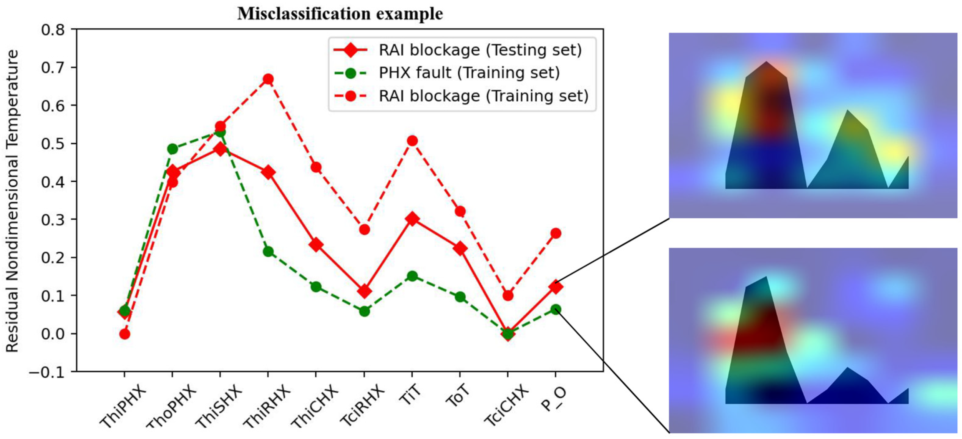
5.2. Specific Case Analysis

Although Grad-CAM has been an effective visual explanation tool to verify that the 2D-CNN TL solution could identify the fault patterns in the target system via distant source domains, another perspective to explain the improvement gained by the 2D-CNN TL solution was to investigate how it avoided the mistakes that the non-TL baseline method made. This was investigated by looking into the specific cases where the non-TL baseline method predicted a false label while the 2D-CNN TL method predicted it correctly. In doing so, the advantage of the 2D-CNN TL solution over the non-TL method could be found, enriching our understanding of the methods.

Still working with the scenario where 15 cases exist in the target training set of ECS, the predictions from the non-TL baseline method and from the 2D-CNN TL method using ImageNet as the source were compared with the true label of each case in the ECS testing set. It was found that the most common cases the 2D-CNN TL solution correctly predicted, while the non-TL baseline could not, were the ram air inlet (RAI) blockage cases. There were 19 such cases, and the non-TL baseline predicted them incorrectly as a PHX fault.

One of the misclassified RAI blockage cases is plotted in Figure 15 (solid red line). To investigate why it achieved incorrect classification, clues could be found by looking into the most similar case in the training set based on which the diagnosis algorithms were trained. From Figure 15, the RAI case in the testing set is actually closer to a PHX fault case in the training set (dashed green line) than the RAI blockage case in the training set (dashed red line). Hence, the non-TL baseline method misclassified the RAI case as a PHX case due to numerical similarity. However, the fact that the 2D-CNN-based TL solution correctly predicted the RAI case in the testing set must imply that it can distinguish it from the PHX case in the training set. Applying Grad-CAM on the two confusing cases revealed such behaviour. As shown in Figure 15, the heatmap for the two confusing cases following the 2D-CNN TL solution has different concentration regions, which means that the TL method detected different patterns in the two images and, hence, correctly identified them as two different classes. Therefore, one advantage of the 2D-CNN TL solution over its non-TL comparison is its ability to overcome numerical similarity and distinguish confusing cases based on minute pattern differences.

5.3. Performance of TL Method over Complex Fault Patterns

A similar explanation could be expected for the improvement in APU diagnostic accuracy from the 2D-CNN TL method, but, as a former section demonstrated, the multiple fault modes brought additional confusion between the cases. Hence, it is worth analysing how well the TL method works on the complex fault patterns for APU multiple fault modes.

The scenario where 34 cases existed in the training set was taken as the scenario of interest, as this was where the accuracy of the 2D-CNN TL solution with ImageNet first reached above 75%. The accuracy for all testing cases, as well as the separate accuracy for the single fault cases and multiple fault cases for the TL method and non-TL baseline, is summarised in

Table 5. Accuracy for APU testing set with 34-case training set.

Method	Average Accuracy over Single Fault Cases Only	Average Accuracy over Multiple Fault Cases Only	Average Accuracy over All Cases
1D CNN non-TL baseline	94.00%	50.00%	72.00%
2D CNN TL: ImageNet–APU	99.33%	52.66%	76.00%

. From Table 5, it is clear that, firstly, multiple fault cases were much more challenging than single fault cases since the accuracy over multiple fault cases was considerably lower than the single faults. Secondly, the TL solution based on 2D-CNN improved the accuracy over both single fault cases and multiple fault cases compared to the non-TL baseline. To determine how the TL method makes better predictions for the multiple fault modes, the predictions from the TL method and the non-TL method were studied for each individual case, and the ones where only the TL method could predict correctly were focused on. These include several cases of the fault mode F11 that the non-TL method wrongly classified as F12, while the TL baseline predicted them correctly. Since the F12 cases have only one more faulty component, it is remarkably similar to the F11 cases. Figure 16 plots a pair of F11 and F12 cases in which the fault profiles are very similar. The similarity of the F11 case with the F12 case numerically causes misclassification for the non-TL baseline. However, Grad-CAM visualisation shows that despite the similarity in the general pattern, the transferred 2D-CNN shows different concentration regions around the minor pattern differences between the two cases, which suggests that it can detect the two cases as having different patterns. Hence, the application of the TL solution based on 2D-CNN has a better capacity over complex fault patterns, owing to the possibility of detecting minute pattern differences.

Although the behaviour of the 2D-CNN TL method to detect minute pattern differences cannot always be expected, the demonstration of such behaviour in both ECS (discussed in Section 5.2) and APU proves that it has an advantage over the non-TL method and can provide an explanation for the accuracy of the improvement.

6. Conclusions and Future Work

6.1. Conclusions

To improve the efficiency of developing fault diagnosis for complex aircraft systems, this work proposed an approach by transferring diagnostic knowledge between vastly different engineering systems. Branches of TL were used with the potential to achieve the transfer between distant and dissimilar domains, and two major directions were attempted, using an analogy or an intermediate domain. Among the three systems of interest, the ECS and APU datasets were selected as the target domain, assuming only a limited number of labelled data was available, and the fuel system was used as the source domain, which was used to pre-train the deep networks. The results of TL-based methods were compared against the results from a 1D-CNN without TL to verify if the knowledge transfer could bring positive benefits for the fault diagnosis.

Using this analogy, the optimal order of target domain features that gave the minimum MMD distance with the source domain features was found, which would suggest an analogical relationship between the source and target domain features. After reordering the target domain features this way, the 1D-CNN pre-trained with the fuel system data was transferred to the ECS and APU datasets, where it was finetuned by the small training set and tested by the testing set. The results show that this TL solution based on 1D-CNN improved the accuracy in the ECS case by over 8%, demonstrating the pattern recognition ability transferred from the fuel system to the ECS. However, it did not improve the APU case, which means the positive transfer benefit is not guaranteed where there are no similar patterns between the two datasets. Hence, an alternative method was considered necessary.

Using an intermediate domain, the image recognition domain, the TL solution based on 2D-CNN was implemented. Because 2D-CNN pre-trained with a large image dataset existed, two source domains were considered: the ImageNet dataset and the fuel system dataset. The transfer from ImageNet to the ECS and APU cases reduced the minimum labelled cases required to reach a high accuracy, from 27 to 15 and from 40 to 34, respectively. The transfer from fuel system data also demonstrated positive benefits for accuracy. These results prove the possibility of using 2D-CNN-based TL to relieve the requirement of large training datasets. In practical terms, the proposed method provides an accurate and efficient diagnosis solution for systems with data scarcity and modelling difficulties, such as aircraft systems and other complex engineering systems. Additionally, using ImageNet-pre-trained 2D-CNN in place of generating a simulation dataset for complex systems in the source domain considerably relieves the workload of developing fault diagnosis algorithms.

Using Grad-CAM to visualise the concentration regions of the ImageNet transferred 2D-CNN when making the predictions, it was found that the concentration regions coincided with the distinct features of each fault mode, which validated the fact that the transfer of pattern recognition ability is the key to improving prediction accuracy compared to the non-TL method. Furthermore, the pattern recognition capacity transferred to the APU case was able to distinguish minute differences between multiple fault modes, which improved the complex fault pattern distinguishing ability. In summary, the cross-system TL solution based on 2D-CNN proposed by this work has demonstrated the possibility and advantage of applying distant domain TL in fault diagnosis, which is one way to improve the efficiency of CBM.

6.2. Future Work

This paper demonstrates the possibility of using cross-system TL methods to improve the diagnostic accuracy of data-scarce systems. However, with distant domain TL still being a rare discussion in IFD, there is a wide range of directions that future work could pursue. From the perspective of key assumptions, one assumption made by this work is the availability of residual data. In reality, it may be hard to collect system data as residual data due to the lack of knowledge of a healthy baseline under each operating condition. Hence, future work could seek ways to design cross-system TL solutions with clustering methods to relieve this assumption. From the perspective of datasets, the future work of cross-system TL on other systems will enrich the discussion. For example, applying cross-system TL between physically similar systems may be a better solution than using ImageNet as the source domain. Alternatively, an image dataset consisting of artificial fault patterns could be created with the sole purpose of pre-training CNNs for optimal fault pattern recognition capacity, i.e., an ideal source domain image dataset, instead of ImageNet, for the 2D-CNN-based TL solution of IFD problems. From an algorithm perspective, other ways to implement cross-system TL could be explored, such as applying other relation-based TL or TTL algorithms to IFD.

References

1. International Air Transport Association (IATA). Airline Maintenance Cost Executive Commentary FY2023 Data [Online]. 2025. Available online: https://www.iata.org/contentassets/bf8ca67c8bcd4358b3d004b0d6d0916f/fy2023-mcx-report_public.pdf (accessed on 15 March 2025).
2. Aviation MRO Spend Grows Amid Rising Costs and Supply Chain [Online]. Available online: https://www.oliverwyman.com/our-expertise/insights/2024/apr/mro-survey-2024-aviation-mro-grows-amid-rising-costs-supply-chain-woes.html (accessed on 18 January 2025).
3. Jennions, I.K. Integrated Vehicle Health Management: Perspectives on an Emerging Field; SAE International: Warrendale, PA, USA, 2011. [Google Scholar] [CrossRef]
4. Verhagen, W.J.C.; Santos, B.F.; Freeman, F.; van Kessel, P.; Zarouchas, D.; Loutas, T.; Yeun, R.C.K.; Heiets, I. Condition-Based Maintenance in Aviation: Challenges and Opportunities. Aerospace 2023, 10, 762. [Google Scholar] [CrossRef]
5. Ezhilarasu, C.M.; Angus, J.; Jennions, I.K. Toward the Aircraft of the Future: A Perspective from Consciousness. J. Artif. Intell. Conscious. 2023, 10, 249–290. [Google Scholar] [CrossRef]
6. Yang, Q.; Zhang, Y.; Dai, W.; Pan, S.J. Transfer Learning; Cambridge University Press: Cambridge, UK, 2020. [Google Scholar] [CrossRef]
7. Zheng, H.; Wang, R.; Yang, Y.; Yin, J.; Li, Y.; Li, Y.; Xu, M. Cross-Domain Fault Diagnosis Using Knowledge Transfer Strategy: A Review. IEEE Access 2019, 7, 129260–129290. [Google Scholar] [CrossRef]
8. Lei, Y.; Yang, B.; Jiang, X.; Jia, F.; Li, N.; Nandi, A.K. Applications of machine learning to machine fault diagnosis: A review and roadmap. Mech. Syst. Signal Process. 2020, 138, 106587. [Google Scholar] [CrossRef]
9. Azari, M.S.; Flammini, F.; Santini, S.; Caporuscio, M. A Systematic Literature Review on Transfer Learning for Predictive Maintenance in Industry 4.0. IEEE Access 2023, 11, 12887–12910. [Google Scholar] [CrossRef]
10. Guo, L.; Lei, Y.; Xing, S.; Yan, T.; Li, N. Deep Convolutional Transfer Learning Network: A New Method for Intelligent Fault Diagnosis of Machines with Unlabelled Data. IEEE Trans. Ind. Electron. 2019, 66, 7316–7325. [Google Scholar] [CrossRef]
11. Li, B.; Zhao, Y.P.; Chen, Y.B. Learning transfer feature representations for gas path fault diagnosis across gas turbine fleet. Eng. Appl. Artif. Intell. 2022, 111, 104733. [Google Scholar] [CrossRef]
12. He, M.; Cheng, Y.; Wang, Z.; Gong, J.; Ye, Z. Fault Location for spacecraft ACS system using the method of transfer learning. In Proceedings of the Chinese Control Conference, CCC, Shanghai, China, 26–28 July 2021; Volume 2021, pp. 4561–4566. [Google Scholar] [CrossRef]
13. Wang, H.; Yang, Q. Transfer learning by structural analogy. In Proceedings of the National Conference on Artificial Intelligence, San Francisco, CA, USA, 7–11 August 2011; Volume 1, pp. 513–518. [Google Scholar]
14. Tan, B.; Song, Y.; Zhong, E.; Yang, Q. Transitive transfer learning. In Proceedings of the ACM SIGKDD International Conference on Knowledge Discovery and Data Mining, Sydney, Australia, 10–13 August 2015; Volume 2015, pp. 1155–1164. [Google Scholar] [CrossRef]
15. Jennions, I.; Ali, F.; Miguez, M.E.; Escobar, I.C. Simulation of an aircraft environmental control system. Appl. Therm. Eng. 2020, 172, 114925. [Google Scholar] [CrossRef]
16. Skliros, C.; Ali, F.; Jennions, I. Experimental investigation and simulation of a Boeing 747 auxiliary power unit. J. Eng. Gas Turbine Power 2020, 142, 081005. [Google Scholar] [CrossRef]
17. Li, J.; King, S.; Jennions, I. Intelligent Multi-Fault Diagnosis for a Simplified Aircraft Fuel System. Algorithms 2025, 18, 73. [Google Scholar] [CrossRef]
18. Jennions, I.; Ali, F. Assessment of heat exchanger degradation in a Boeing 737-800 environmental control system. J. Therm. Sci. Eng. Appl. 2021, 13, 061015. [Google Scholar] [CrossRef]
19. Jia, L.; Ezhilarasu, C.M.; Jennions, I.K. Cross-Condition Fault Diagnosis of an Aircraft Environmental Control System (ECS) by Transfer Learning. Appl. Sci. 2023, 13, 13120. [Google Scholar] [CrossRef]
20. Skliros, C.; Ali, F.; Jennions, I. Fault simulations and diagnostics for a Boeing 747 Auxiliary Power Unit. Expert Syst. Appl. 2021, 184, 115504. [Google Scholar] [CrossRef]
21. Zhang, D.; Zhou, T. Deep Convolutional Neural Network Using Transfer Learning for Fault Diagnosis. IEEE Access 2021, 9, 43889–43897. [Google Scholar] [CrossRef]
22. Shao, S.; McAleer, S.; Yan, R.; Baldi, P. Highly Accurate Machine Fault Diagnosis Using Deep Transfer Learning. IEEE Trans. Ind. Inf. 2019, 15, 2446–2455. [Google Scholar] [CrossRef]
23. Ruhi, Z.M.; Jahan, S.; Uddin, J. A novel hybrid signal decomposition technique for transfer learning based industrial fault diagnosis. Ann. Emerg. Technol. Comput. 2021, 5, 37–53. [Google Scholar] [CrossRef]
24. Liu, J.; Hou, L.; Zhang, R.; Sun, X.; Yu, Q.; Yang, K.; Zhang, X. Explainable fault diagnosis of oil-gas treatment station based on transfer learning. Energy 2023, 262, 125258. [Google Scholar] [CrossRef]
25. ImageNet [Online]. Available online: https://www.image-net.org/ (accessed on 21 October 2024).
26. He, K.; Zhang, X.; Ren, S.; Sun, J. Deep Residual Learning for Image Recognition. In Proceedings of the IEEE Computer Society Conference on Computer Vision and Pattern Recognition, Las Vegas, NV, USA, 27–30 June 2016; pp. 770–778. [Google Scholar] [CrossRef]
27. Pedregosa, F.; Michel, V.; Grisel, O.; Blondel, M.; Prettenhofer, P.; Weiss, R.; Vanderplas, J.; Cournapeau, D.; Varoquaux, G.; Gramfort; et al. Scikit-Learn: Machine Learning in Python. J. Mach. Learn. Res. 2011, 12, 2825–2830. [Google Scholar]
28. Keras. Deep Learning for Humans [Online]. Available online: https://keras.io/ (accessed on 21 October 2024).
29. Selvaraju, R.R.; Cogswell, M.; Das, A.; Vedantam, R.; Parikh, D.; Batra, D. Grad-CAM: Visual Explanations from Deep Networks via Gradient-based Localization. Int. J. Comput. Vis. 2016, 128, 336–359. [Google Scholar] [CrossRef]
30. Brito, L.C.; Susto, G.A.; Brito, J.N.; Duarte, M.A.V. Fault Diagnosis using eXplainable AI: A transfer learning-based approach for rotating machinery exploiting augmented synthetic data. Expert Syst. Appl. 2023, 232, 120860. [Google Scholar] [CrossRef]
Figure 1. Schematic of B737-800 PACK [18].
Applsci 15 03232 g001
Figure 2. Plot of ECS-representative cases.
Applsci 15 03232 g002
Figure 3. Schematic of APU for B747-100/200/300 [20].
Applsci 15 03232 g003
Figure 4. Plot of APU-representative cases.
Applsci 15 03232 g004
Figure 5. Schematic of fuel system [17].
Applsci 15 03232 g005
Figure 6. Plot of fuel system-representative cases.
Applsci 15 03232 g006
Figure 7. Methodology: overall TL scheme, a solution based on 1D-CNN, and a solution based on 2D-CNN.
Applsci 15 03232 g007
Figure 8. An example showing the idea of structural analogy [6].
Applsci 15 03232 g008
Figure 9. An illustration of TTL [6].
Applsci 15 03232 g009
Figure 10. Image preparation process.
Applsci 15 03232 g010
Figure 11. Result from conventional ML methods without TL for (a) the ECS case; (b) the APU case.
Applsci 15 03232 g011
Figure 12. Result from TL solution based on 1D-CNN for (a) the ECS case; (b) the APU case.
Applsci 15 03232 g012
Figure 13. Results from TL solution based on 2D-CNN for (a) the ECS case; (b) the APU case.
Applsci 15 03232 g013
Figure 14. Plot of Grad-CAM heatmaps superimposed on the input image of an (a) ACM fault case; (b) RAI blockage case; (c) TCV fault case; (d) healthy case; (e) PHX fault case; and (f) SHX fault case.
Applsci 15 03232 g014
Figure 15. Plot of the misclassified case in the testing set with the confusing case in the training set and same-label case in the training set.
Applsci 15 03232 g015
Figure 16. Grad-CAM visualisation plot for the confusing cases: F11 (left) and F12 (right).
Applsci 15 03232 g016