Time-Specified Adaptive Robust Control Framework for Managing Nonlinear System Uncertainties

Abstract

This paper addresses the issue of prescribed-time control for a specific class of uncertain nonlinear systems. Initially, a stability theorem based on prescribed time is introduced, utilizing adaptive techniques for the first time. Building on this theorem, a novel state feedback control approach is presented, employing the backstepping method for high-order nonlinear systems with unknown parameters to ensure convergence within the prescribed time. Furthermore, the proposed prescribed-time controller is derived in the form of continuous time-varying feedback, enabling all system states to converge to zero within the specified time. Notably, the prescribed time is independent of the system’s initial conditions, allowing it to be set arbitrarily within the physical constraints. Finally, two simulation examples are provided to demonstrate the effectiveness of the proposed algorithm.

1. Introduction

Finite-time control has drawn increasing attention from scholars in recent decades owing to its faster convergence rate [1]. The concept of finite-time control first appeared in [2] for the purpose of achieving time-optimal control. Afterward, non-smooth feedback control methods were utilized to ensure finite-time stabilization [3,4]. Unfortunately, due to the presence of negative fractional powers and discontinuous terms, singularities and chattering may arise in the system’s operating process [5], which significantly restricts the practical application of sliding mode finite-time control as, for example, in missile guidance [6]. To address these issues, a classical finite-time control theorem grounded in “Lyapunov’s differential inequality” was initially developed in [7], and further investigated in [8]. The findings from [7,8] have been extended to a variety of systems, including double-integrator systems [9], time-varying dynamical systems [10], general nonlinear systems [11], stochastic systems [12], and multiagent systems [13]. The homogeneous approach was introduced in [14,15]. Additionally, notable achievements in the finite-time stabilization of partial differential equations (PDEs) were presented in [16,17].

Although finite-time control strategies have been broadly studied, their settling time is dependent on initial conditions [18]. Furthermore, in numerous real-world applications, it can be difficult or even impossible to know the system’s initial values in advance, making control of the settling time infeasible. Consequently, the work in [5] developed a fixed-time control algorithm where the upper bound of the settling time does not depend on initial conditions. Follow-up results for fixed-time control concerning certain linear and nonlinear systems were provided in [1,19,20]. The fixed-time stabilization issue for reaction–diffusion PDEs was resolved in [21] by employing a continuous boundary time-varying feedback control strategy. While current fixed-time stabilization results can drive system states to zero within a desired time by selecting appropriate control parameters, achieving convergence at an arbitrary time remains extremely challenging [22]. Recently, the problem of predefining the upper bound of the settling time in fixed-time stabilization, also known as predefined-time stabilization, was examined in [22,23,24,25]. In these references, one can freely choose the upper bound of the settling time by suitably configuring control parameters. Nevertheless, the actual convergence time in predefined-time stabilization still hinges on the initial conditions, which distinguishes it from prescribed-time stabilization results [26], where the actual convergence time is independent of initial conditions.

Research on prescribed-time stabilization has been reported in [25,26,27,28,29,30,31,32,33,34,35]. In [25,27], through a state-scaling approach (the time-varying function in the scaling goes to infinity as time nears the prescribed end time), the global prescribed-time stabilization problem for nonlinear systems in strict-feedback form was solved. The advantages of prescribed-time regulation over finite-time regulation were highlighted in [28]. In [29], a sufficient condition was presented to guarantee convergence within an arbitrary time, and a novel prescribed-time control strategy for linear systems was introduced. By employing the backstepping technique, [30] successfully tackled the prescribed-time stabilization of reaction–diffusion PDEs. Using a decoupling backstepping approach, [31] accomplished prescribed-time trajectory tracking for triangular systems of reaction–diffusion PDEs. The most recent development on prescribed-time stabilization for reaction–diffusion PDEs can be found in [32]. In [33], several Lyapunov-like prescribed-time stability theorems were provided and compared with certain finite-time stability theorems. Grounded in the Lyapunov-like function, [26] addressed the global prescribed-time stabilization of a class of nonlinear systems. The prescribed-time stabilization of strict-feedback systems and stochastic systems (where the nonlinear function meets a linear growth condition) was studied in [34,35], respectively.

Prescribed-time control presents a significant advancement over finite-time and fixed-time control methodologies. Unlike finite-time control, where convergence time depends on initial conditions, or fixed-time control, which provides an upper bound independent of initial conditions, prescribed-time control achieves exact convergence at a specified time regardless of initial conditions. This precise temporal specification is particularly valuable in mission-critical applications requiring coordination between multiple systems or processes. Mathematically, prescribed-time control employs time-varying feedback structures that introduce a time-dependent scaling factor, often in the form of ${\displaystyle \frac{1}{(T_p-t)}}$, where $T_p$ is the prescribed convergence time. This factor ensures that the system states reach equilibrium exactly at $t$ = $T_p$, after which a different control strategy maintains the system at equilibrium.

It is widely recognized that precisely modeling a system in practice can be very difficult. Adaptive Control offers a functional avenue to tackle nonlinear systems with uncertain parameters by estimating unknown parameters online [36]. Many well-known adaptive designs for uncertain nonlinear systems have been proposed (see [37,38,39]). However, due to estimation errors, Barbalat’s lemma—commonly employed in Adaptive Control—cannot be directly utilized for the stability analysis of finite/prescribed-time control [36]. Current adaptive finite/prescribed-time control results generally fall into two categories. The first ensures the convergence of system states to a neighborhood of the equilibrium point or to a defined compact set within a finite time (refer to [40,41]); the second guarantees that the system states converge to the equilibrium point within a finite interval (refer to [36,42]). Obviously, the latter is more challenging, yet more meaningful. Hence, this article concentrates on the latter issue. In [36], global adaptive finite-time control was investigated for a class of nonlinear systems in p-normal form with parametric uncertainties. From this earlier work, it is evident that the finite/fixed-time control methods based on “Lyapunov’s differential inequality” in [5,7] are not immediately applicable to systems with uncertain parameters. Meanwhile, [42,43,44] achieved adaptive prescribed-time stabilization for uncertain nonlinear systems using the dynamic high-gain scaling approach. Nevertheless, because the time-varying function is applied to scale the states in all coordinate transformations, the computational load involving the derivative of the scaling function grows considerably [35]. Moreover, prescribed-time stabilization is particularly significant in tackling transient problems; its benefits align well with numerous applications that impose strict time constraints, such as missile interception. Yet the majority of controlled systems demand that the state reaches the origin within the prescribed time and remains there—aircraft autonomous rendezvous and docking, and unmanned aerial vehicles arriving at designated locations, are prime examples. Under these conditions, it is imperative not only to ensure finite-time convergence but also to maintain the system at the origin post-convergence.

While the proposed adaptive prescribed-time control strategy effectively handles parameter uncertainties, real-world systems frequently encounter disturbances, unmodeled dynamics, and noise that can degrade performance or even destabilize the closed-loop system if not addressed. Therefore, incorporating robust control principles into this research is essential to further ensure stability and performance within the prescribed time bound, even under significant external perturbations.

A robust extension of the proposed methodology would involve designing the control law and adaptation mechanisms to accommodate bounded disturbances and uncertainties more systematically. For instance, techniques like sliding-mode observers, H-infinity filters, or disturbance observers could be integrated to estimate and compensate for perturbations without substantially increasing the controller’s computational requirements. Additionally, selecting robust Lyapunov-like functions that include disturbance attenuation terms would allow the stability analysis to account explicitly for exogenous inputs. By blending Adaptive Control with robust control design, the resulting framework would not only guarantee convergence within a prescribed time but also maintain stability and desired performance levels in the face of unforeseen challenges, thereby broadening the applicability of the approach in diverse engineering systems. Based on the above considerations, the principal contributions are summarized below.

For a class of uncertain nonlinear systems, this work introduces a novel adaptive prescribed-time stability theorem for the first time. Drawing on this theorem, an innovative state feedback control strategy is derived using adaptive techniques and the backstepping method. Notably, the prescribed time is independent of the system’s initial conditions and can be specified to meet practical requirements.

In contrast to the state-scaling design approach (which involves a time-varying function that diverges as time approaches the prescribed limit), our method does not utilize this time-varying function in the state transformations; rather, it is selectively incorporated into the controller design. Even relative to the most recent prescribed-time stabilization findings, our proposed control strategy can notably decrease the computational complexity.

Previous prescribed-time stabilization results developed through temporal transformations and state-scaling design are defined only on a finite time horizon and thus cannot be naturally extended to infinity. Conversely, we devise an Adaptive Control scheme here that extends the time interval to infinity.

Based on the above considerations, the principal contributions of this work are as follows:

Novel theoretical framework: We introduce an adaptive prescribed-time stability theorem for uncertain nonlinear systems, establishing the theoretical foundation for guaranteed convergence within a specified timeframe.

Innovative control design: We derive a state feedback control strategy using adaptive techniques and the backstepping method that ensures all system states converge to zero within the prescribed time, independent of initial conditions.

Computational efficiency: Unlike state-scaling approaches where time-varying functions appear in state transformations, our method selectively incorporates these functions only in the controller design, significantly reducing computational complexity.

Extended time interval: We devise an Adaptive Control scheme that naturally extends beyond the prescribed time horizon to infinity, overcoming limitations of previous approaches that are defined only on finite time intervals.

Robust enhancement: We augment the Adaptive Controller with robust components to effectively handle unmodeled dynamics and external disturbances, demonstrated through comparative simulations.

The remainder of this paper is structured as follows: Section 2 provides background on relevant control methodologies including Adaptive Control, Sliding Mode Control, Finite-Time Control, and Fixed-Time Control, along with comparisons to observer-based methods and recent SMC approaches. Section 3 presents the methodology of our proposed adaptive robust prescribed-time control framework, detailing the controller design, stability analysis, and implementation considerations. Section 4 demonstrates the effectiveness of the proposed approach through two simulation examples, comparing results with existing methods. Finally, Section 5 concludes the paper and discusses future research directions.

2. Background and Related Work

Adaptive Control is a method employed to manage uncertainties in system parameters and environmental variations [45,46]. For uncertain nonlinear systems, Adaptive Control adjusts the controller parameters in real-time to achieve the desired performance. In short, Adaptive Control can be classified into three types: MRAC, self-tuning, and gain scheduled. The first one, MRAC, is based on a stability perspective, with stability theory as its foundation. The second, self-tuning control, is grounded in an optimization perspective, originating from the first Self-Tuning Regulators (STRs) and controllers. Finally, gain scheduling is an approach to controlling nonlinear systems that employs a family of linear controllers, each designed to ensure satisfactory control at different operating points of the system. Adaptive Control encompasses two main strategies frequently discussed in the literature: Model Reference Adaptive Control (MRAC) and Self-Tuning Regulator Control (STRC).

2.1. Adaptive Control

Adaptive Control is a method employed to manage uncertainties in system parameters and environmental variations. For uncertain nonlinear systems, Adaptive Control adjusts the controller parameters in real-time to achieve the desired performance. Adaptive Control encompasses two main strategies: Model Reference Adaptive Control (MRAC) and Self-Tuning Regulator Control (STRC). In Model Reference Adaptive Control (MRAC) [47], a reference model is established to describe the desired behavior of the system. The controller parameters are adjusted so that the actual system output aligns with the reference output. These parameters are continuously updated in real-time to accommodate any changes in the system, with stability typically ensured by employing Lyapunov-based methods. Self-Tuning Regulator Control (STRC) directly estimates and adjusts the controller parameters to account for uncertainties within the system. Adaptive Control offers significant advantages in handling uncertainties in system parameters and adapting to environmental changes, which makes it an extremely versatile approach. However, its design for nonlinear systems can be quite complex, and challenges may arise regarding the convergence of parameter estimation. Despite these challenges, Adaptive Control is extensively used across various industries, such as aerospace, autonomous driving, unmanned vehicles, and robotics, particularly for systems with dynamic or fluctuating parameters.

2.2. Sliding Mode Control (SMC)

Sliding mode control (SMC) is a widely utilized robust control technique for nonlinear systems, known for its effectiveness in handling model uncertainties and external disturbances. The fundamental concept behind SMC is to create a sliding surface that compels the system to move along it, ensuring both system stability and the fulfillment of performance criteria. In this approach, a sliding surface (or sliding hyperplane) is initially defined, usually as a function of the system’s states:

$$S\left(x\right)=Cx+d=0$$

(1)

In this context, $S\left(x\right)$ represents the sliding surface, while C and d are design parameters. The control law employs a switching control strategy to drive the system state to move along the sliding surface. A typical expression for the sliding mode control law is

$$u\left(t\right)=-k·sign\left(S\left(x\right)\right)$$

(2)

where $k$ represents a sufficiently large positive control gain, and $sign\left(S\left(x\right)\right)$ denotes the sign function of $S\left(x\right)$.

Sliding mode control (SMC) offers significant advantages, particularly its high robustness, which enables it to effectively handle uncertainties in system parameters, external disturbances, and input constraints. However, one of its primary drawbacks is the “chattering” phenomenon, which involves high-frequency oscillations near the sliding surface. Despite this limitation, sliding mode control is widely utilized in various uncertain nonlinear systems, such as robotic control, spacecraft control, and autonomous driving.

2.3. Finite-Time Control

Finite-time control is a control approach aimed at ensuring a system reaches a specific target, such as achieving zero stability, within a fixed period. The objective of finite-time control is to design a control strategy that ensures the system’s state converges to the desired state within a predetermined and finite time frame. This method commonly utilizes Lyapunov stability theory in conjunction with appropriate control strategies to guarantee convergence within the set time. The Lyapunov function frequently employed in such approaches is

$$V\left(x\right)={\displaystyle \frac{1}{2}}{x}^{T}Px$$

(3)

where $P$ represents a positive definite matrix. The control law is developed to ensure that the time derivative of the Lyapunov function is negative, thereby meeting the conditions for finite-time convergence.

Finite-Time Control offers the advantage of ensuring that the system reaches the desired state within a fixed period, making it especially useful for control tasks that demand quick responses. However, for systems with considerable uncertainties, a more robust control design may be required to achieve finite-time convergence. This approach is extensively used in fields where fast and precise responses are essential, including flight control, mobile robotics, and process control.

2.4. Fixed-Time Control

Fixed-time control is an emerging method that ensures the system reaches the desired state within a predetermined time, independent of the system’s initial conditions or external disturbances. Unlike finite-time control, which ensures convergence within a finite time but where the convergence time depends on the initial state, fixed-time control guarantees that the time to reach the target is fixed. This control approach is designed through a control law that guarantees the system will achieve the desired state in a fixed time. It utilizes appropriate Lyapunov functions and mathematical techniques to ensure that the convergence time remains constant. The main benefit of fixed-time control is that it provides a reliable and fixed time to reach the target state, regardless of the initial conditions.

Fixed-time control offers a significant advantage by ensuring convergence to the target state within a predetermined time, regardless of the system’s initial conditions. This characteristic distinguishes it from finite-time control, where the settling time is influenced by the initial state. However, the implementation of fixed-time control involves a more complex design process, requiring a thorough understanding of the system’s dynamics and parameters to achieve accurate controller tuning and effectively manage uncertainties. Due to its ability to provide rapid and precise control, fixed-time control is particularly well-suited for high-performance applications. These include spacecraft attitude regulation, unmanned vehicle operations, and real-time control systems that necessitate strict response times and robustness within a fixed time frame.

2.5. Comparison with Observer-Based Methods

Recent advancements in observer-based methods for nonlinear systems have shown promising results in handling uncertainties. Notably, the works presented in references [48,49] utilize intermediate observers to estimate unknown states and disturbances. However, prescribed-time control offers several advantages over these methods:

Time specification: Unlike observer-based methods which typically provide asymptotic convergence, prescribed-time control guarantees convergence within a user-defined time interval, regardless of initial conditions.

Robustness to initial conditions: Observer-based methods often require accurate initial state estimates, whereas prescribed-time control maintains consistent performance across varying initial conditions.

Computational efficiency: The proposed approach avoids the need for separate observer design and implementation, potentially reducing computational overhead.

Adaptability: Our method combines adaptive techniques with prescribed-time control, allowing simultaneous parameter estimation and robust control within the specified timeframe.

Deterministic performance: While observer-based methods typically provide statistical guarantees of performance, prescribed-time control offers deterministic convergence guarantees.

2.6. Comparison with Recent SMC Approaches

Recent work on “Improved Sliding Mode Tracking Control for Spacecraft Electromagnetic Separation Supporting On-orbit Assembly” [50] has demonstrated significant advancements in SMC techniques for specific aerospace applications. This approach uses a boundary layer technique to reduce chattering and implements adaptive gains to handle uncertainties. While effective, it differs from our prescribed-time approach in several key aspects:

Convergence guarantees: The improved SMC approach provides asymptotic stability, whereas our prescribed-time controller guarantees convergence at exactly the specified time.

Parameter adaptation: Both approaches implement parameter adaptation, but our method specifically designs the adaptation law to ensure the prescribed-time convergence property is maintained.

Post-convergence behavior: Our approach explicitly addresses system behavior after the prescribed time, ensuring continued stability without additional control redesign.

Robustness implementation: While both approaches incorporate robust terms, our method combines saturation and hyperbolic tangent functions to simultaneously achieve chattering reduction and precise tracking.

Application scope: The improved SMC is specifically optimized for spacecraft operations, whereas our approach provides a more general framework applicable to a broader class of nonlinear systems.

3. Method

This research paper upgrades the controller to bring about higher efficiency based on the controller proposed in reference [44]. Consider a nonlinear system with unknown parameters represented as

$$\dot{x}\left(t\right)=f\left(t,x\left(t\right),u\left(t\right),\theta \right)$$

(4)

In this process, we aim to design an adaptive prescribed-time controller for a specified time $T_p$, breaking the design into two cases: $0\le t<T_p$ and $t\ge T_p$.

We start by introducing a state transformation:

$$z_1=x_1,z_i=x_i-{\alpha }_{i-1},i=2,\dots ,n$$

(5)

where ${\alpha }_{i-1}$ is the virtual controller to be designed later.

Before proceeding, we select the Lyapunov function as follows:

$$V=V_1+V_2$$

(6)

where $V_1$ and $V_2$ are defined as

$$V_1=\sum _{j=1}^n z_j^2,V_2={\tilde{\theta }}^T{\mathrm{\Gamma }}^{-1}\tilde{\theta }$$

(7)

with $\bar{\theta }=\theta -\hat{\theta },\hat{\theta }$ being the estimated value of $\theta$, and $\mathrm{\Gamma }$ a positive definite matrix. Using the properties of the Lyapunov function, it can be shown that $V,V_1$, and $V_2$ satisfy the conditions outlined in above.

The controller is developed using the backstepping approach, consisting of $n$ steps. For the derivative of $z_1$, we have the following:

$${\dot{z}}_1=z_2+{\alpha }_1+{\theta }^T{f}_1$$

Thus, the virtual controller ${\alpha }_1$ is designed as follows:

$${\alpha }_1=-{\sigma }_1{\displaystyle \frac{z_1}{T_p-t}}-{\hat{\theta }}^T{f}_1$$

(8)

where ${\sigma }_1>n$ is a design parameter. Then, the derivatives of $z_1$ and $W_1=z_1^2+V_2$ are given by the following:

$${\dot{z}}_1=-{\sigma }_1{\displaystyle \frac{z_1}{T_p-t}}+{\mathrm{\Omega }}_1$$

(9)

$${\dot{W}}_1=-2{\sigma }_1{\displaystyle \frac{z_1^2}{T_p-t}}+2z_1{z}_2+2{\bar{\theta }}^T\left({\tau }_1-{\mathrm{\Gamma }}^{-1}\dot{\hat{\theta }}\right)$$

(10)

where ${\mathrm{\Omega }}_1=z_2+{\bar{\theta }}^T{f}_1$ and ${\tau }_1=z_1{f}_1$.

For the derivative of $z_2$, we have

$${\dot{z}}_2=z_3+{\alpha }_2+{\theta }^T{f}_2-{\displaystyle \frac{\partial {\alpha }_1}{\partial \hat{\theta }}}\dot{\hat{\theta }}-{\displaystyle \frac{\partial {\alpha }_1}{\partial x_1}}\left(x_2+{\theta }^T{f}_1\right)-{\displaystyle \frac{\partial {\alpha }_1}{\partial t}}$$

(11)

The virtual controller ${\alpha }_2$ is then designed as follows:

$${\alpha }_2=-{\sigma }_2{\displaystyle \frac{z_2}{T_p-t}}-z_1-{\hat{\theta }}^T{f}_2+{\displaystyle \frac{\partial {\alpha }_1}{\partial \hat{\theta }}}\mathrm{\Gamma }{\tau }_2+{\displaystyle \frac{\partial {\alpha }_1}{\partial x_1}}\left(x_2+{\hat{\theta }}^T{f}_1\right)+{\displaystyle \frac{\partial {\alpha }_1}{\partial t}}$$

(12)

where ${\tau }_2={\tau }_1+z_2\left(f_2-{\displaystyle \frac{\partial {\alpha }_1}{\partial x_1}}{f}_1\right)$ and ${\sigma }_2>n-1$ is a design parameter. The derivatives of $z_2$ and $W_2=W_1+z_2^2$ are the following:

$${\dot{z}}_2=-{\sigma }_2{\displaystyle \frac{z_2}{T_p-t}}+{\mathrm{\Omega }}_2$$

(13)

$${\dot{W}}_2=-2\sum _{j=1}^2 {\sigma }_j{\displaystyle \frac{z_j^2}{T_p-t}}+2{\tilde{\theta }}^T\left({\tau }_2-{\mathrm{\Gamma }}^{-1}\dot{\hat{\theta }}\right)+2{\displaystyle \frac{\partial {\alpha }_1}{\partial \hat{\theta }}}{z}_2\left(\mathrm{\Gamma }{\tau }_2-\dot{\hat{\theta }}\right)+2z_2{z}_3$$

(14)

where ${\mathrm{\Omega }}_2=z_3-z_1+{\tilde{\theta }}^T{f}_2+{\displaystyle \frac{\partial {\alpha }_1}{\partial \dot{\theta }}}\left(\mathrm{\Gamma }{\tau }_2-\dot{\hat{\theta }}\right)-{\displaystyle \frac{\partial {\alpha }_1}{\partial x_1}}{\tilde{\theta }}^T{f}_1$.

For $z_i$, the derivative is the following:

$${\dot{z}}_i=z_{i+1}+{\alpha }_i+{\theta }^T{f}_i-{\displaystyle \frac{\partial {\alpha }_{i-1}}{\partial \hat{\theta }}}\dot{\hat{\theta }}-{\displaystyle \frac{\partial {\alpha }_{i-1}}{\partial t}}-\sum _{j=1}^{i-1} {\displaystyle \frac{\partial {\alpha }_{i-1}}{\partial x_j}}\left(x_{j+1}+{\theta }^T{f}_j\right)$$

(15)

The virtual controller ${\alpha }_i$ is designed as below:

$${\alpha }_i=-{\sigma }_i{\displaystyle \frac{z_i}{T_p-t}}-z_{i-1}-{\hat{\theta }}^T{f}_i+{\displaystyle \frac{\partial {\alpha }_{i-1}}{\partial t}}+\sum _{j=1}^{i=1} {\displaystyle \frac{\partial {\alpha }_{i-1}}{\partial x_j}}\left(x_{j+1}+{\hat{\theta }}^T{f}_j\right)+{\displaystyle \frac{\partial {\alpha }_{i-1}}{\partial \hat{\theta }}}\mathrm{\Gamma }{\tau }_i+\sum _{j=1}^{i=1} {\displaystyle \frac{\partial {\alpha }_{i-1}}{\partial x_j}}{f}_j\mathrm{\Gamma }$$

(16)

where ${\tau }_i={\tau }_{i-1}+z_i\left(f_i-{\sum }_{j=1}^{i-1} {\displaystyle \frac{\partial {\alpha }_{i-1}}{\partial x_j}}{f}_j\right)$ and ${\sigma }_i>n-i+1$ is a design parameter.

The derivatives of $z_i$ and $W_i=W_{i-1}+z_i^2$ are as follows:

$${\dot{z}}_i=-{\sigma }_i{\displaystyle \frac{z_i}{T_p-t}}+{\mathrm{\Omega }}_i$$

(17)

$${\dot{W}}_i=-2\sum _{j=1}^i {\sigma }_j{\displaystyle \frac{z_j^2}{T_p-t}}+2{\tilde{\theta }}^T\left({\tau }_i-{\mathrm{\Gamma }}^{-1}\dot{\hat{\theta }}\right)+2\sum _{j=2}^{i-1} {\displaystyle \frac{\partial {\alpha }_j}{\partial \hat{\theta }}}{z}_j\left(\mathrm{\Gamma }{\tau }_i-\dot{\hat{\theta }}\right)+2z_i{z}_{i+1}$$

(18)

where

$${\mathrm{\Omega }}_i=z_{i+1}-z_{i-1}+{\tilde{\theta }}^T{f}_i+{\displaystyle \frac{\partial {\alpha }_{i-1}}{\partial \hat{\theta }}}\left(\mathrm{\Gamma }{\tau }_i-\dot{\hat{\theta }}\right)-\sum _{j=1}^{i-1} {\displaystyle \frac{\partial {\alpha }_{i-1}}{\partial x_j}}{\tilde{\theta }}^T{f}_j+\left(f_i-\sum _{j=1}^{i-1} {\displaystyle \frac{\partial {\alpha }_{i-1}}{\partial x_j}}{f}_j\right)\mathrm{\Gamma }.$$

For $z_n$, the derivative is as follows:

$$\dot{z_n}=u+{\theta }^T{f}_n-{\displaystyle \frac{\partial {\alpha }_{n-1}}{\partial \hat{\theta }}}\dot{\hat{\theta }}-{\displaystyle \frac{\partial {\alpha }_{n-1}}{\partial t}}-\sum _{j=1}^{n-1} {\displaystyle \frac{\partial {\alpha }_{n-1}}{\partial x_j}}\left(x_{j+1}+{\theta }^T{f}_j\right)$$

(19)

The controller $u$ and adaptive law are designed as follows:

$$u=-{\hat{\theta }}^T{f}_n+\mathrm{\Phi }\left({\bar{x}}_n,t\right)$$

(20)

$$\dot{\hat{\theta }}=\mathrm{\Gamma }{\tau }_n$$

(21)

where ${\tau }_n={\tau }_{n-1}+z_n\left(f_n-{\sum }_{j=1}^{n-1} {\displaystyle \frac{\partial {\alpha }_{n-1}}{\partial x_j}}{f}_j\right),{\sigma }_n>1$ is a design parameter, and

$$\mathrm{\Phi }=-{\sigma }_n{\displaystyle \frac{z_n}{T_p-t}}-z_{n-1}+{\displaystyle \frac{\partial {\alpha }_{n-1}}{\partial t}}+{\displaystyle \frac{\partial {\alpha }_{n-1}}{\partial \hat{\theta }}}\mathrm{\Gamma }{\tau }_n+\sum _{j=1}^{n-1} {\displaystyle \frac{\partial {\alpha }_{n-1}}{\partial x_j}}\left(x_{j+1}+{\hat{\theta }}^T{f}_j\right)+\left(f_n-\sum _{j=1}^{n-1} {\displaystyle \frac{\partial {\alpha }_{n-1}}{\partial x_j}}{f}_j\right)\mathrm{\Gamma }$$

(22)

Finally, we have the below:

$${\dot{z}}_n=-{\sigma }_n{\displaystyle \frac{z_n}{T_p-t}}+{\mathrm{\Omega }}_n$$

(23)

$$\dot{V}={\dot{W}}_n\le -2\mu \left(t\right)V_1$$

(24)

where ${\mathrm{\Omega }}_n$ is a complex expression, and $\mu (t)={\sigma }_1{\displaystyle \frac{1}{T_p-t}}$ is a prescribed-time function. For $t\ge T_p$, the control signal and adaptive law are set to

$$u=0,\dot{\hat{\theta }}=0$$

(25)

In cases with large or rapidly varying uncertainties, a robust term is added to the original controller. The standard procedure for defining $z_1,{\alpha }_1,z_2$, and ${\mathrm{\Phi }}_1$ remains unchanged, but the final control law includes a supplementary term:

$$\mathrm{robust}\_\mathrm{term} =-k_r\left[0.5\mathrm{s}\mathrm{a}\mathrm{t}\left({\displaystyle \frac{z_2}{ϵ}}\right)+0.5\mathrm{t}\mathrm{a}\mathrm{n}\mathrm{h}\left(10z_2\right)\right]$$

(26)

where $k_r$ is the robust gain, $ϵ$ is the boundary layer thickness, $\mathrm{s}\mathrm{a}\mathrm{t}\left(s\right)$ is the saturation function, and $\mathrm{t}\mathrm{a}\mathrm{n}\mathrm{h}\left(s\right)$ smooths transitions near the boundary manifold. This results in the updated control law:

$$u=-{\displaystyle \frac{{\sigma }_2{z}_2}{T_p-t}}+{\mathrm{\Phi }}_1+ \mathrm{robust}\_\mathrm{term}$$

(27)

This improves the system’s robustness to external disturbances and modeling inaccuracies. The adaptive law for $\hat{\theta }$ continues to estimate uncertain parameters, preserving the backstepping structure while reducing chattering and extreme control signals.

A similar approach is applied in the following section, where a robust block is added after finalizing the nominal design. The backstepping errors and virtual controls ${\alpha }_i$ remain, and the final control action incorporates a robust component using saturation and tanh.

For unmodeled uncertainties, a robust component is added:

$$u_{\mathrm{robust} }=-k_r\left[0.5\mathrm{s}\mathrm{a}\mathrm{t}\left({\displaystyle \frac{z_i}{ϵ}}\right)+0.5\mathrm{t}\mathrm{a}\mathrm{n}\mathrm{h}\left(10z_i\right)\right]$$

(28)

where

$$\mathrm{s}\mathrm{a}\mathrm{t}(s)=\left\{\begin{array}{ll}\mathrm{s}\mathrm{i}\mathrm{g}\mathrm{n}\left(s\right),& \left|s\right|>1\\ s,& \left|s\right|\le 1\end{array}\right.$$

$ϵ$ is a parameter to avoid excessive chattering, $k_r$ is the robust gain, and $\mathrm{t}\mathrm{a}\mathrm{n}\mathrm{h}\left(s\right)$ smooths the control signal near the sliding manifold boundary.

Thus, the enhanced control law becomes

$$u=-{\displaystyle \frac{{\sigma }_i{z}_i}{T_p-t}}+{\varphi }_{i-1}-k_r\left[0.5\mathrm{s}\mathrm{a}\mathrm{t}\left({\displaystyle \frac{z_i}{ϵ}}\right)+0.5\mathrm{t}\mathrm{a}\mathrm{n}\mathrm{h}\left(10z_i\right)\right]$$

(29)

The relationship between parameter selection and control performance is crucial in prescribed-time control. The design parameters ${\sigma }_{\mathrm{i}} (i=1, 2, ...,n)$ directly influence the convergence rate and robustness. Higher values of σᵢ accelerate convergence but may lead to increased control effort and potential chattering. The prescribed time $Tₚ$ must be selected according to physical system constraints and desired performance metrics. Meanwhile, the robust gain $kᵣ$ and boundary layer thickness $\epsilon$ in Equation (28) control the trade-off between robustness to uncertainties and the smoothness of the control signal. Smaller values of ε provide tighter tracking but may increase chattering, while larger values smoothen the control signal at the cost of tracking precision. Our simulations demonstrate that setting $\sigma ᵢ>n-i+1$, with moderate robust gain $kᵣ$, provides an optimal balance between convergence speed and control effort.

This ensures backstepping-style stability while handling unmodeled uncertainties and disturbances.

The novelty in this upgrade is the addition of a robust term into the control law, which helps the system maintain high stability and more accurate control when facing unmodeled uncertainties or large disturbances. This robust term is built from saturation and tanh functions, which smooth the control signal, minimize large oscillations, and reduce chattering. This helps limit unwanted oscillations, creates more stable control signals, and improves the system’s ability to withstand sudden changes in the operating environment. This upgrade is based on Adaptive Control theory and Lyapunov theory to ensure that the control signals and adaptive laws continue to maintain the stability and convergence of the system, even in the presence of parameter variations or disturbances. The control structure still retains the backstepping method, but with important improvements that allow the system to adapt better and remain more stable under changing conditions. The adaptability of this upgrade is clearly demonstrated through the reduction in chattering and maintaining control accuracy, especially when dealing with rapid or uncertain parameter changes in the system. The addition of the robust term allows the system to operate more effectively without requiring significant changes to the basic control structure, making it easier to apply to real-world systems.

The backstepping-based design employed in our approach offers several key advantages for uncertain nonlinear systems:

• Improved global stability: It enables the handling of nonlinear systems in a structured manner, ensuring stability at each design step.
• Reduction in chattering: Smooth Lyapunov functions can be designed, using approximations such as tanh(s) instead of sign(s), thereby mitigating undesired chattering effects.
• More precise control: Compared to traditional SMC, the backstepping approach offers more refined control, avoiding abrupt discontinuities in the control signal.
• Greater flexibility: It is useful in systems where standard SMC cannot be applied directly due to physical or structural constraints.
• However, this approach also presents certain challenges:
• Computational complexity: The backstepping design introduces additional differential equations, increasing the computational burden.
• Sensitivity to unstructured uncertainties: While it enhances robustness against parametric uncertainties, it may not be as effective if the uncertainty has high temporal variability.
• Practical implementation challenges: In real-world applications, backstepping design requires precise state and parameter estimation, which can be challenging in noisy systems or those with delays.

Our robust enhancement mitigates several of these limitations, particularly through the introduction of the composite saturation–tanh function that balances robustness and control smoothness.

4. Results and Discussion

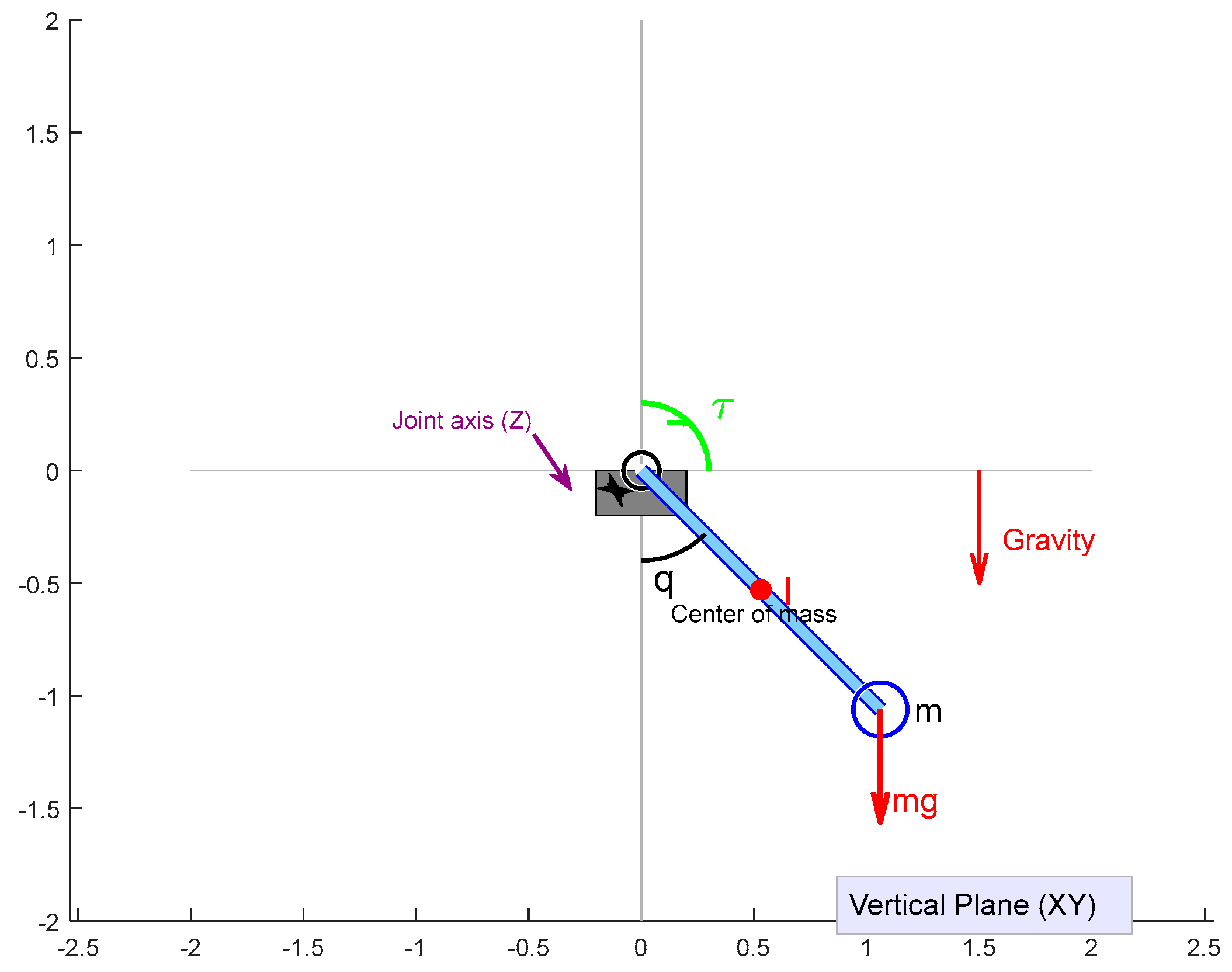
4.1. Example 1: Single-Link Manipulator Model

The first model describes the dynamics of a single-link manipulator with an uncertain parameter. Figure 1 illustrates the schematic representation of this system.

The first model describes the dynamics of a single-link manipulator with an uncertain parameter.

The state equation for this system is

$$M\ddot{q}+\omega \dot{q}+{\displaystyle \frac{1}{2}}mgl\mathrm{s}\mathrm{i}\mathrm{n}(q)=\tau$$

where q, $\dot{q}$, and $\ddot{q}$ represent the angular position, velocity, and acceleration of the link, respectively. The parameter $M$ is the moment of inertia, $\omega$ is the viscous friction coefficient at the joint, $\tau$ is the control torque, and $m, l$, and $g$ represent the mass, the length of the link, and gravitational acceleration, respectively. The gravitational term $mgl·sin\left(q\right)$ appears because the manipulator operates in a vertical plane, where gravity exerts a moment on the link proportional to $sin\left(q\right)$. This term creates a nonlinear effect that varies with the angular position, making control more challenging.

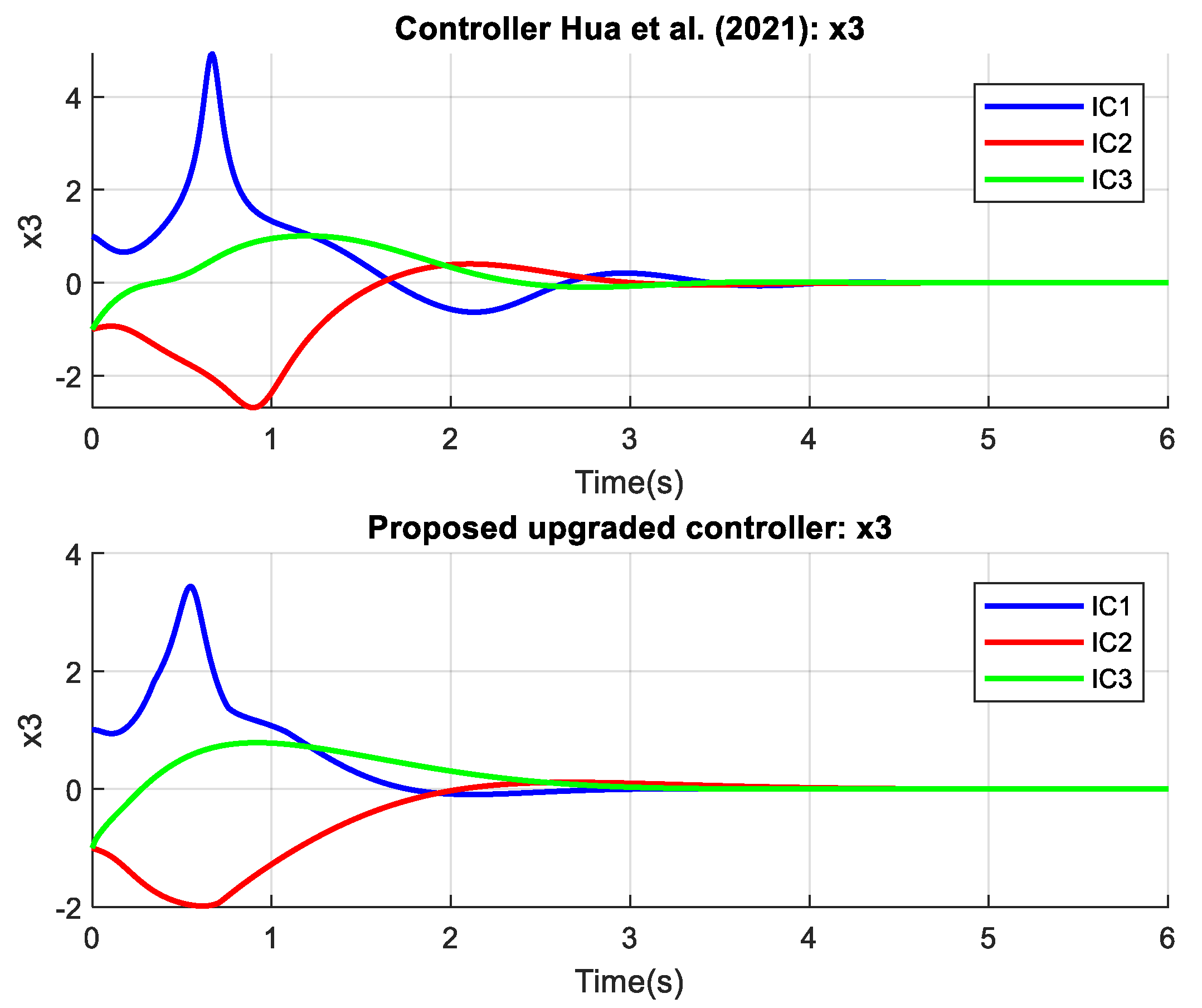
4.2. Example 2: Third-Order Uncertain Parameter System

The second model is a third-order system with uncertain parameters, governed by the following dynamic equations:

$$\begin{array}{c}{\dot{x}}_1=x_2+\theta x_1\\ {\dot{x}}_2=x_3\\ {\dot{x}}_3=u+\theta x_3^2\end{array}$$

Figure 2 illustrates the schematic representation of this system.

In this model, $x_1,x_2$, and $x_3$ represent the system states, $u$ is the control input, and $\theta$ is the uncertain parameter. This system exemplifies a third-order nonlinear system with uncertain dynamics, illustrating the challenges in practical control scenarios.

This system structure appears in various practical applications, including aircraft pitch dynamics, certain chemical reactor models, and flexible joint robotic manipulators. For instance, in aircraft pitch control, $x_1$ might represent the pitch angle, $x_2$ the pitch rate, $x_3$ the derivative of pitch rate, and $\theta$ an uncertain aerodynamic parameter that varies with flight conditions. The nonlinear term $\theta x_3^2$ captures the nonlinear aerodynamic effects that become significant at higher rates of motion.

The relationship between parameter selection methods and control performance in prescribed-time Adaptive Control systems is clearly demonstrated through the intricate interplay between key parameters and the system’s operational characteristics. The parameters σᵢ (i = 1, 2, 3), physically interpreted as smoothing coefficients, directly influence the convergence rate of the corresponding states. Larger values of σᵢ accelerate convergence but simultaneously increase the control signal amplitude, potentially inducing oscillations, whereas smaller σᵢ values yield smoother, albeit slower, convergence with a more refined control signal. Lyapunov stability theory establishes lower bounds for the following parameters: σ₁ > n, σ₂ > n−1, …, σₙ > 1, where n denotes the system order. For a third-order system, this implies σ₁ > 3, σ₂ > 2, and σ₃ > 1. Additionally, the prescribed time $T_p$ plays a critical role in determining when the system reaches the desired state. A smaller $T_p$ accelerates convergence but requires a larger control signal, risking actuator saturation, while a larger $T_p$ prolongs convergence time but reduces control effort, minimizing actuator fatigue. A notable advantage of this approach is that the actual convergence time precisely matches $T_p$, independent of initial conditions.

In an enhanced version of the controller, the robust gain coefficient $k_r$ and the boundary layer parameter ε collectively form a robust component that significantly influences the trade-off between accuracy and signal smoothness. A larger $k_r$ enhances robustness against disturbances and uncertainties but may introduce chattering, while a smaller $k_r$ produces a smoother control signal at the expense of reduced robustness. Similarly, a larger ε mitigates chattering but compromises accuracy, whereas a smaller ε improves accuracy but heightens the risk of chattering. From the baseline control equation $u=-{\displaystyle \frac{{\sigma }_3{z}_3}{T_p-t}}+{\varphi }_2-k_r\left[0.5\mathrm{s}\mathrm{a}\mathrm{t}\left({\displaystyle \frac{z_3}{ϵ}}\right)+0.5\mathrm{t}\mathrm{a}\mathrm{n}\mathrm{h}\left(10z_3\right)\right]$, it is evident that an increase in σ₃ amplifies the term $-{\displaystyle \frac{{\sigma }_3{z}_3}{T_p-t}}$, resulting in greater control energy. Simulations reveal that elevating σ₃ from 1.5 to 5 can increase control energy by up to 40%, though it also enhances convergence speed. Analysis of the expression ${\displaystyle \frac{{\sigma }_i{z}_i}{T_p-t}}$ indicates that as t approaches $T_p$, the denominator approaches zero, causing a sharp increase in control signal amplitude. However, since zᵢ also tends toward zero, a sufficiently large $T_p$ can achieve a favorable balance between convergence speed and smoothness. Simulations with $T_p$ = 2 s and $T_p$ = 5 s demonstrate that the peak control signal for $T_p$ = 2 s is approximately 80% higher than for $T_p$ = 5 s, with the latter yielding a smoother signal but extended convergence time.

The robust component, governed by $k_r$ and ε, further shapes system behavior. Frequency spectrum analysis reveals that with $k_r$ = 0.5 and ε = 0.2, high-frequency components are low (approximately 15 dB/Hz) but robustness diminishes, whereas with $k_r$ = 2.0 and ε = 0.05, high-frequency components rise (approximately 22 dB/Hz), improving robustness. Based on theoretical and experimental analyses, an effective parameter selection procedure begins with determining $T_p$ according to application requirements and actuator physical constraints. Subsequently, σᵢ values are initialized at their minimum thresholds per Lyapunov stability and incrementally adjusted to enhance convergence speed within acceptable control signal limits, with recommended values of σ₁ ≈ 1.5 n, σ₂ ≈ 1.5(n−1), and σ₃ ≈ 1.5. For the enhanced controller, $k_r$ and ε are then tuned, starting with a small $k_r$ and moderate ε. $k_r$ is increased if greater disturbance rejection is needed, while ε is adjusted upward to reduce excessive chattering or downward to improve accuracy.

In practice, parameter selection involves balancing conflicting objectives such as high accuracy, rapid response, and smooth control signals tailored to specific application demands. Depending on whether the priority is precision, responsiveness, or signal refinement, parameters can be adjusted accordingly to optimize control performance, ensuring an effective compromise between convergence speed, accuracy, and smoothness.

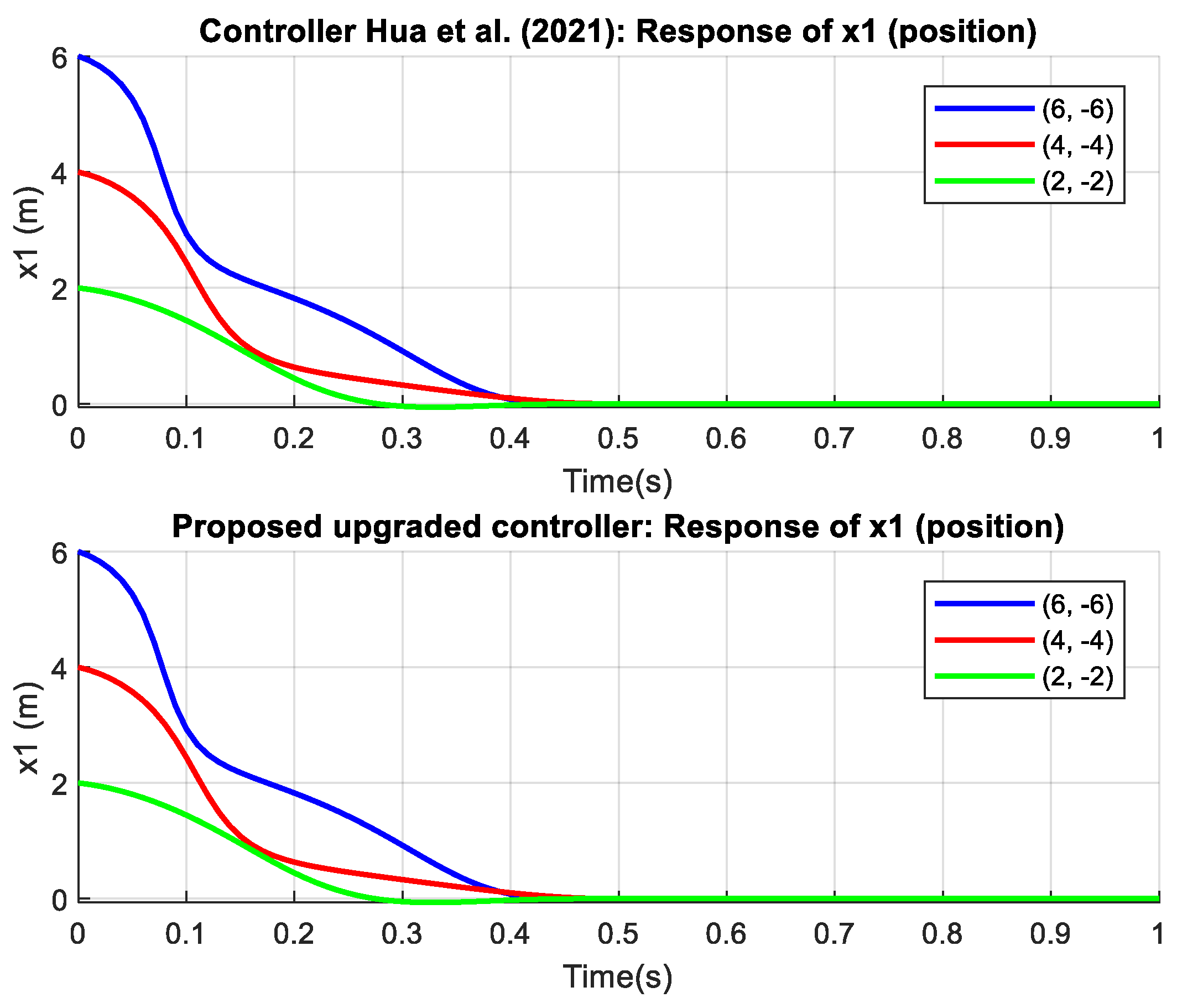
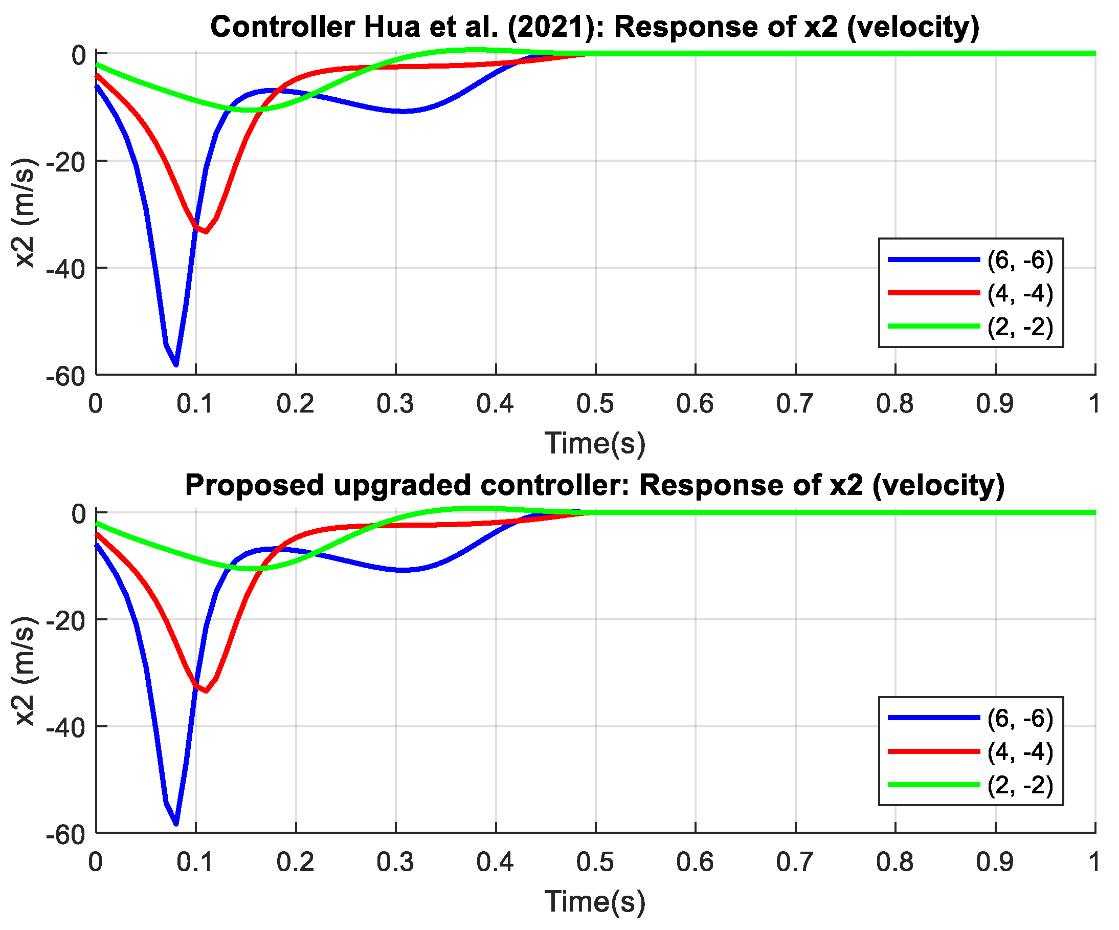
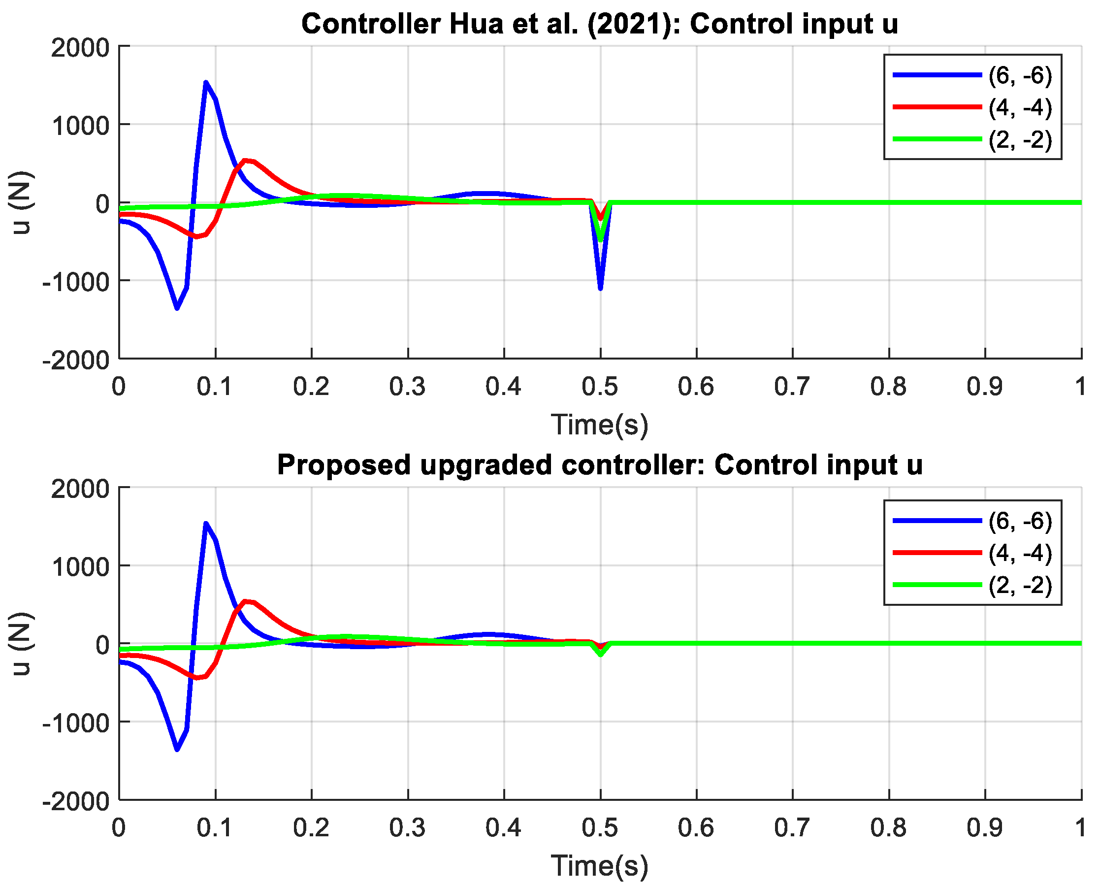
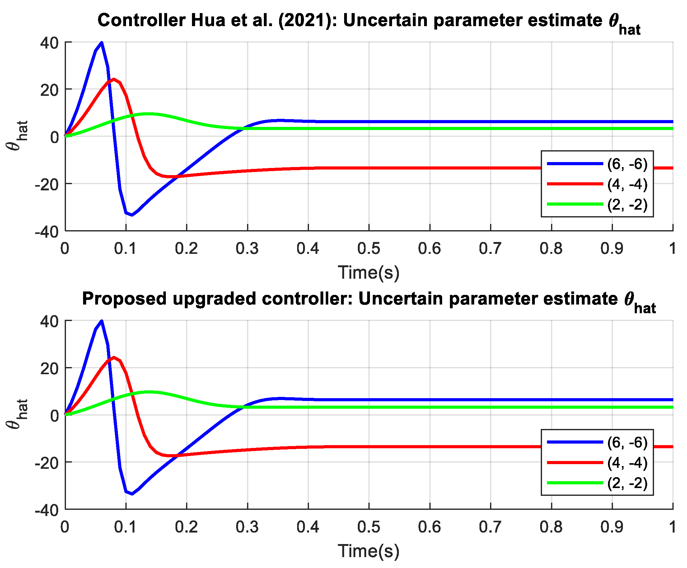
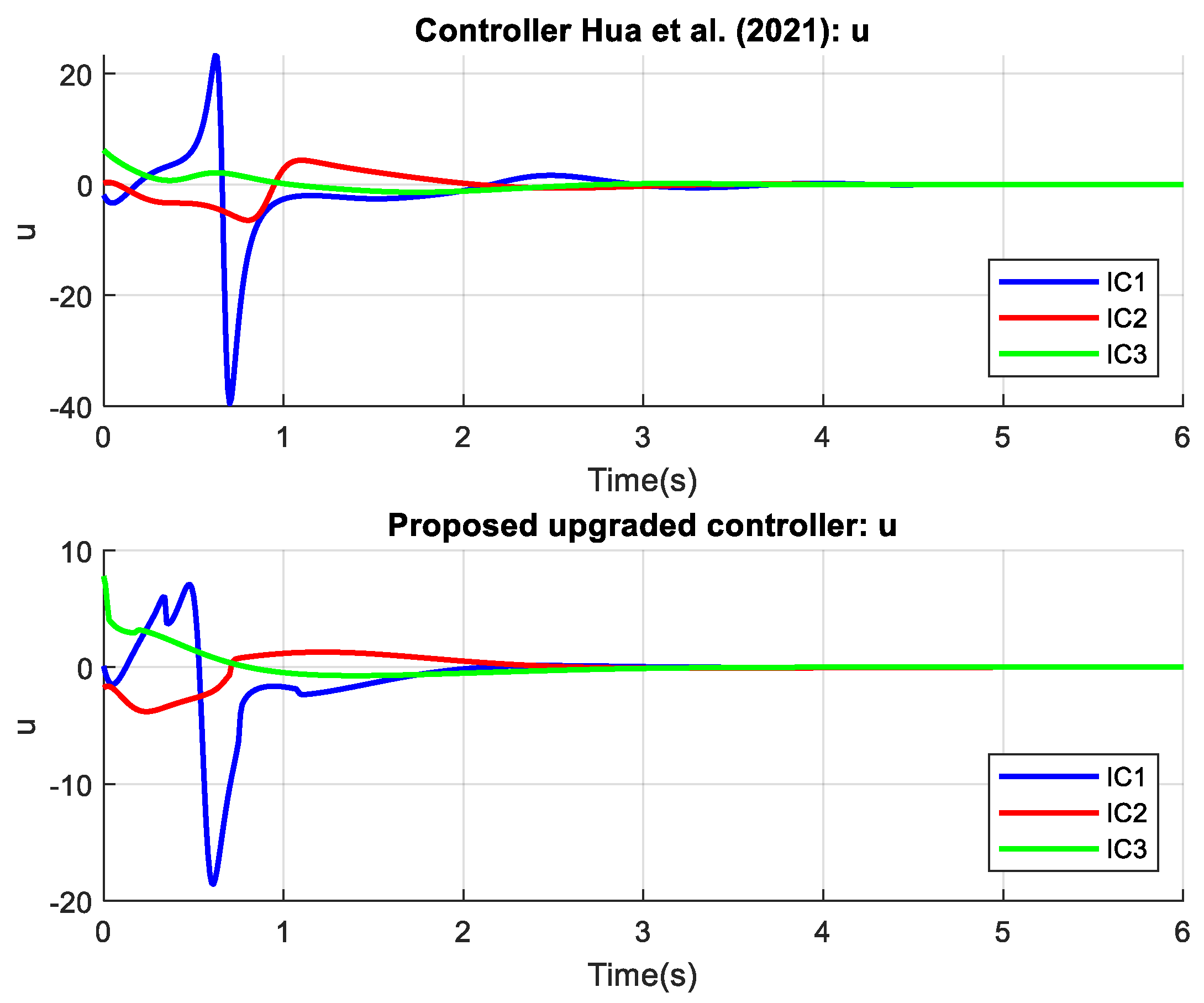
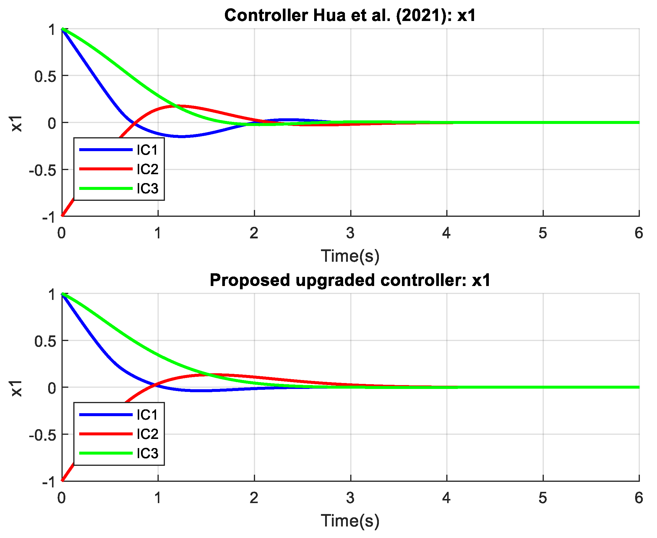
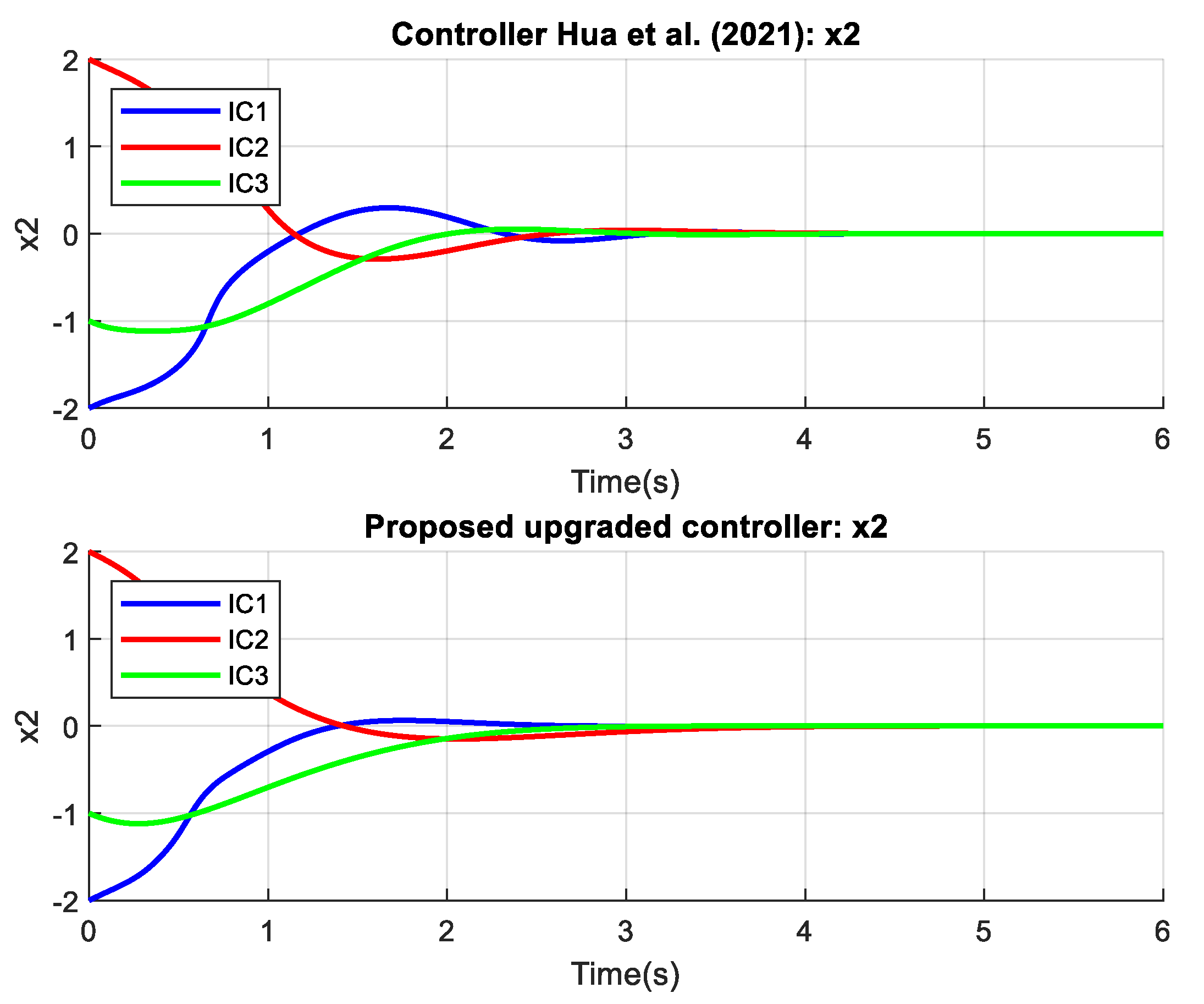
The proposed controller outperforms the controller from reference [44] in terms of speed, accuracy, and smoothness of convergence for both examples and all states. The main advantages of the proposed controller are its faster stabilization times, reduced oscillations, and smaller control efforts, ensuring a more efficient and robust response across different initial conditions. The proposed controller also excels in estimating uncertain parameters. The results from Figure 3, Figure 4, Figure 5 and Figure 6 represent the outcomes from Example 1, where Figure 3 and Figure 4 show nearly equivalent curves and timing, making it difficult to discern differences. However, Figure 5, which depicts the control signal, clearly demonstrates the difference and superiority of the proposed controller, exhibiting a smoother curve with less noise and volatility. The superiority and excellence of the proposed controller are even more pronounced in Example 2, shown in Figure 7, Figure 8, Figure 9 and Figure 10, where the signal curves of the proposed controller are distinctly smoother, while the controller from reference [44] produces more oscillatory signals. These results indicate that the proposed controller is more reliable and effective compared to the previous controller. Future developments will continue to focus on reducing human influence and computation, aiming for further advancements in control methods.

5. Conclusions

This paper addresses the problem of adaptive robust prescribed-time control for a class of uncertain nonlinear systems. The concept of prescribed-time stability is first introduced. Subsequently, a new adaptive prescribed-time convergence theorem is proposed to enable adaptive robust prescribed-time control. Building on this result, a time-varying state feedback controller is designed for uncertain nonlinear systems, ensuring that all states reach zero within a specified timeframe. Moreover, this prescribed time is independent of initial conditions and can be chosen arbitrarily. Future investigations will focus on expanding prescribed-time control methods to more general uncertain nonlinear systems.

It is worth noting that control effort is traditionally one of the drawbacks of Adaptive Control methods. However, our proposed controller successfully reduces the control effort compared to the approach in reference [44], as clearly demonstrated in Figure 5 and Figure 7. This reduction in control effort, combined with improved robustness and guaranteed convergence time, makes the proposed approach particularly suitable for practical implementations where actuator limitations must be considered.

Future investigations will focus on expanding prescribed-time control methods to more general uncertain nonlinear systems, including those with input constraints, time delays, and higher-order dynamics. Additionally, we plan to explore the integration of learning-based approaches to further enhance adaptability to unmodeled dynamics and time-varying disturbances.