Abstract
Sustainable transport is an important trend in smart cities to achieve sustainability development goals. It refers to the use of transport modes with low emissions, energy consumption and negative impacts on the environment. Ridesharing is one important sustainable transport mode to attain the goal of net zero greenhouse gas emissions. The discount-guaranteed ridesharing problem (DGRP) aims to incentivize drivers and riders and promote ridesharing through the guarantee of a discount. However, the computational complexity of the DGRP poses a challenge in the development of effective solvers. In this study, we will study the effectiveness of creating new self-adaptive differential evolution (DE) algorithms based on an old saying to solve the DGRP. Many old sayings still have far-reaching implications today. Some of them influence the organization of management teams for companies and decisions to improve performance and efficiency. Whether an old saying that works effectively for human beings to solve problems can also work for developers to create effective optimization problem solvers in the realm of artificial intelligence is an interesting research question. In our previous study, one self-adaptive algorithm was proposed to solve the DGRP. This study demonstrates how to create a series of self-adaptive algorithms based on the old saying “Two heads are better than one” and validates the effectiveness of this approach based on experiments and comparison with the algorithms proposed previously. The new finding of this study is that the old saying not only works effectively for human beings to solve problems but also works effectively in the creation of new scalable and robust self-adaptive algorithms to solve the DGRP. In other words, the old saying provides a simple and systematic approach to the development of effective optimization problem solvers in artificial intelligence.
1. Introduction
As a transport mode enabling reduction of the number of vehicles in use, energy consumption and emissions of greenhouse gas in cities, shared mobility has drawn researchers’ and practitioners’ attention around the world. Many transport service providers such as Uber [1] and Lyft [2] have implemented shared mobility systems. Shared mobility has led to the creation of a lot of studies in the ridesharing literature [3,4,5]. In the past years, various ridesharing problems with different models were studied. Recently, ridesharing with multiple platforms was considered in [6] to match supply and demand across multiple platforms to improve the overall revenue of platforms through coordination. The study [7] aims to determine efficient routes and schedules for drivers and passengers with flexible pick-up and delivery locations. Motivated by the need to reduce CO2 emissions, a graph-theoretical algorithm-based approach was proposed to achieve higher levels of reduction in CO2 emissions in the study [8]. A review of the challenges and opportunities due to shared mobility is available in [9,10,11].
Financial benefits provide one strong incentive for the prevailing ridesharing model. In the literature, cost savings due to ridesharing make it possible for drivers and riders to reduce their travel cost and enjoy the monetary incentives in shared mobility systems. In the literature, different mechanisms have been developed to incentivize ridesharing drivers and riders. These include cost sharing [12], discounting [13] and cost allocation [14,15]. In [12], a general cost sharing framework to create cost sharing mechanisms with desirable properties and compensation for inconvenience costs due to detours was proposed and validated based on a real case study. In [13], a non-linear mixed integer optimization problem to maximize the profit and offer shared trips to riders with varying price discounts was proposed. The problem was decomposed into two sequential sub-problems to achieve computation efficiency. Results of experiments confirm that the dynamic discount strategy produces substantial economic benefits.
As cost savings are a benefit of shared mobility that provides one financial incentive to riders, many studies focus on maximization of cost savings in shared mobility systems. However, if the amount of cost savings is insufficient to attract riders, riders will not accept the ridesharing mode [14]; proper allocation of cost savings can help improve the acceptability of ridesharing [15]. For this reason, the study [16] formulated a discount-guaranteed ridesharing problem (DGRP) to ensure a minimal discount for drivers and riders in ridesharing systems. Due to the complexity of a DGRP, metaheuristic algorithms have been developed in [16] to find solutions.
Metaheuristic algorithms refer to algorithms that are characterized by imitating natural phenomena or human intelligence and are able to tackle the complexity issue in solving optimization problems. Natural phenomena or human intelligence can be applied to develop effective strategies to guide the process to search solutions efficiently. In the metaheuristics literature, many metaheuristic algorithms were proposed by drawing inspiration from natural phenomena, biological sciences, laws of physics, rules of games and human activities. In the study [17], metaheuristic algorithms are classified into five categories: physics-based, swarm-based, evolutionary-based, game-based and human-based methods. In the remainder of this section, we will first give a brief review of these categories. Then we will focus on the issue to create metaheuristic algorithms based on the saying “Two heads are better than one”.
1.1. Literature Review of Categories of Metaheuristic Algorithms
Simulated annealing and the gravitational search algorithm (GSA) are two examples of metaheuristic algorithms based on physics. Simulated annealing is based on the physical process of annealing in which materials are heated and cooled slowly to decrease defects and minimize the system energy [18]. The GSA [19] is inspired by Newton’s law of gravity and motion. In the GSA, agents are modeled as objects. The performance of an object is measured by its mass. Objects attract each other due to gravity force. Gravity force makes all objects move toward heavier objects. An object with heavier mass corresponds to a better solution.
Swarm-based metaheuristic algorithms are developed based on the concept of swarm intelligence, which refers to the collective learning and decision-making behavior of self-organized entities in natural or artificial systems. Well-known examples of swarm-based metaheuristic algorithms include particle swarm optimization (PSO) [20], the firefly algorithm (FA) [21], artificial bee colony (ABC) [22], ant colony optimization (ACO) [23], etc. ACO is a metaheuristic inspired by the foraging behavior of ant colonies. A variety of strategies are used by ants to forage for food. One strategy is to leave pheromones to mark their path to food. Ants mark some favorable paths by depositing pheromones on the ground. These favorable paths are followed by other ants of the colony to facilitate selection of the shortest route with the help of the pheromone. PSO is an approach inspired by the social behavior and movement of organisms in a bird flock. The standard PSO algorithm is initiated by creating a population of solutions called particles. Each particle adjusts its position and velocity according to its individual personal best solution and the global best solution to improve the solution. If a particle finds an improved solution that outperforms the current personal best solution, the improved solution will replace the personal best solution. Similarly, if the improved solution found by the particle outperforms the current global best solution, the improved solution will replace the global best solution. The PSO algorithm repeats the above process until the termination condition is satisfied. The flashing characteristics of fireflies inspired the creation of the FA: one firefly attracts another one according to attractiveness proportional to the brightness which decreases as their distance increases, where the brightness of a firefly depends on the objective function. A firefly will move randomly in case it cannot find a brighter one.
Evolutionary-based metaheuristic algorithms mimic the phenomena of biological evolution which is similar to the natural selection theory introduced by Darwin. They borrow the reproduction, mutation, recombination and selection mechanisms from biological evolution to evolve the potential solutions. The genetic algorithm (GA) [24] and differential evolution (DE) [25] are two widely used evolutionary algorithms. The GA starts with a population of candidate solutions (called individuals). Evolution is an iterative process and each iteration is called a generation. For every individual, its fitness is evaluated based on the fitness function of the optimization problem. The population in a generation evolves through applying a combination of genetic operations, including crossover and mutation to form a new generation, to attempt to create better solutions. The GA selects the most fit individuals stochastically from the current population to play the role of parents. An individual in the next generation may be created by applying crossover operations to combine two parents or applying mutation rules to individual parents. The GA terminates either after a maximum number of generations has been executed or the solution quality has reached a satisfactory fitness level. The DE algorithm includes the operations of initialization, mutation, crossover and selection to iteratively improve the solution quality. In the initialization step, a population of individuals is generated. In the mutation step, a mutation strategy is applied to generate a mutant vector for each individual in the population. The crossover step generates a trial vector based on the mutant vector and the original individual. In the selection step, the trial vector will replace the original individual if it is better than the original individual.
Game-based metaheuristic algorithms simulate the behavior of different entities such as players, coaches and other individuals in games and the behavior of different entities is governed by the underlying rules of the games. Football game-based optimization (FGBO) [26] and the volleyball premier league (VPL) algorithm [27] are two well-known examples of game-based metaheuristic algorithms. In FGBO, a population of clubs is generated initially, where each club consists of a number of players. The algorithm calculates the power of each club and determines the best club. It then iteratively follows a procedure with four phases: (a) league holding, (b) player transfer, (c) practice and (d) promotion and relegation to update the status of the clubs and improve the solution quality until the termination condition is satisfied. The VPL algorithm is inspired by the coaching process during a volleyball match. In a volleyball game, a team consists of players, substitutes and the coach. The formulation of a team includes several active players in the active part and standby players in the passive part. A coach decides whether to replace an active player with a standby player in the passive part. The algorithm determines the winning team and the losing team based on the power index and applies different strategies to update the best team. The algorithm removes the k-worst teams, adds new teams to the league, applies the transfer process and updates the best team iteratively until the termination condition is satisfied.
Human-based metaheuristic algorithms are developed based on inspiration from human activities. Examples of human-based metaheuristic algorithms include teaching–learning-based optimization (TLBO) [28], poor and rich optimization (PRO) [29], human mental search (HMS) [30] and driving training-based optimization (DTBO) [17]. TLBO is a population-based algorithm and consists of two phases: Teacher Phase and Learner Phase. The algorithm learns from the teacher in the Teacher Phase whereas it learns through the interaction between learners in the Learner Phase to improve the quality of solutions. PRO is a multi-population-based algorithm. It is inspired by the mechanisms that are used by the poor and the rich to improve their economic situation. Initially, there are two populations: a rich population and a poor population. Each individual in the poor population tries to improve his/her status and reduce the gap between the rich population and poor population by learning from an individual in the rich population. Each individual in the rich population tries to increase the gap between the rich population and poor population by observing them and acquiring wealth. The rich population and poor population are updated after all the individuals have taken actions to try to improve their status. HMS is inspired by strategies to explore the bid space in online auctions. It simulates human behavior in online auctions and consists of three steps: (1) the mental search for exploring around each solution, (2) grouping bids to determine a promising region and (3) moving the bids toward the best strategy. DTBO is inspired by the learning process in a driving school. It is divided into three phases: (1) training by the driving instructor, (2) patterning of students from instructor skills and (3) practice. The best individuals selected from the population play the role of driving instructors and the rest play the role of learner drivers. In the training in the driving instructor phase, a learner driver must choose the driving instructor and learns from that instructor. In the patterning of students from instructor skills phase, each learner driver imitates the instructor to attempt to improve his/her driving skills. In the practice phase, a learner driver tries to achieve his/her best skills through practice.
1.2. Creating Metaheuristic Algorithms Based on a Saying
Besides human activities, sayings or proverbs created by human beings still have far-reaching implications today. An example is the saying “Two heads are better than one”. Although it is believed that the origin of the saying “Two heads are better than one” could be traced back to 1390, it was first recorded in John Heywood’s Book of Proverbs in 1546. This saying can be applied to create new ideas and solve problems. An example is “brainstorming”, which is a group problem-solving method in which each member of the group suggests as many ideas as possible based on his/her expertise and can be regarded as one way to apply this saying to create new ideas or solution methods. Extended results of this saying can be found in the study of [31], which demonstrates that a multi-agent system has the potential to improve the generation of scientific ideas. This saying also influences the organization of management teams for companies as well as the way to effectively make decisions to improve performance and efficiency. An example is multi-agent reinforcement learning [32], where complex tasks that are difficult for a single agent to handle can be completed by a set of agents cooperatively.
The saying “Two heads are better than one” can be interpreted as “two people working together are better than one working alone” [33]. In [33], it is shown that pair programming improves software quality. This saying can also be used to describe the situation in which performing tasks using two systems is better than using only one [34]. This saying may also be applied to confirm the correctness of a conclusion by assigning two teams to perform experiments. For example, in [35], two studies with different data collection processes, databases and data analysis methods were performed to confirm that the trends detected are in general agreement. Finally, this saying may be interpreted as solving a complex problem with two stages may be better than one single stage by dividing it into multiple sub-problems. For example, a divide-and-conquer strategy was used in [36] to divide the original complex problem into multiple sub-problems to reduce complexity.
Whether the above old saying that works effectively for human beings to solve problems can also work for developers to create effective optimization problem solvers in the realm of artificial intelligence is an interesting research question. One way to apply this saying to create an effective optimization problem solver for solving the ridesharing problem is to combine two existing metaheuristic approaches. In the study [37], the author showed how to apply the above saying to create a more efficient metaheuristic algorithm for solving the ridesharing problem based on the hybridization of FA with PSO. However, no self-adaptation mechanism is applied in the approach of [37]. In the study [38], the author demonstrated how to apply the above saying to create new self-adaptive metaheuristic algorithms for solving the ridesharing problem with trust requirements based on the use of the two mutation strategies arbitrarily selected from a set of existing standard DE algorithms. The study [38] first describes how this saying can be applied by humans to solve a problem. The process consists of two phases: the performance assessment phase and optimization phase. The performance assessment phase aims to assess the performance of the two heads for solving the problem. The optimization phase aims to solve the optimization problem based on the performance of the two heads. By mimicking the process to apply this saying, the developed self-adaptive metaheuristic algorithms also consist of two phases: the performance assessment phase and optimization phase. The study [38] validates the effectiveness of applying this saying to develop two-head self-adaptive metaheuristic algorithms. The results indicate that the performance of each two-head self-adaptive metaheuristic algorithm outperforms that of two corresponding “single-head” metaheuristic algorithms. This confirms that this saying provides a simple yet effective approach to the development of effective self-adaptive algorithms for ridesharing systems with trust requirements. However, the effectiveness of the self-adaptive metaheuristic algorithms developed based on this saying might depend on the problem. Although this approach has been validated for the ridesharing problem with trust requirements, whether it can work effectively for other problems is an interesting research question.
In this study, we loosely define a two-head self-adaptive metaheuristic algorithm with two mutation strategies developed by applying “Two heads are better than one” as effective if it outperforms two single-head mutation strategy metaheuristic algorithms. Based on this definition, we will validate whether the approach based on this saying is effective for another problem—the DGRP. To achieve this goal, several two-head self-adaptive metaheuristic algorithms with two mutation strategies have been developed based on this saying. Each two-head self-adaptive metaheuristic algorithm developed based on this saying takes advantage of the two mutation strategies according to their success rates in improving the solutions. A mutation strategy (head) with a higher success rate in improving the solutions will have a higher probability of being selected to solve the given problem. On the contrary, a mutation strategy (head) with a lower success rate in improving the solutions will have a lower probability of being selected to solve the given problem. The two-head self-adaptive metaheuristic algorithm works by applying the two mutation strategies according to their historical success rates to improve the solutions. The two-head self-adaptive metaheuristic algorithm iterates in the optimization phase until the termination criteria are satisfied. An important issue is the design of the fitness function for the two-head self-adaptive metaheuristic algorithms. We adopt the approach of [39] to take into account the objective function and constraints in the fitness function to effectively move toward the feasible region through biasing feasible solutions against infeasible ones by penalizing the violation of constraints.
To fully validate the effectiveness of the two-head self-adaptive metaheuristic algorithms developed for the DGRP, we considered a set of four mutation strategies and arbitrarily selected any combination of two mutation strategies from the set to develop the two-head self-adaptive metaheuristic algorithms. This results in six two-head self-adaptive metaheuristic algorithms. To validate the effectiveness of each of the six two-head self-adaptive metaheuristic algorithms, we conducted experiments to compare the performance of each two-head self-adaptive metaheuristic algorithm with the corresponding two single-head metaheuristic algorithms. We analyzed the results to illustrate the effectiveness of applying the above saying to develop two-head self-adaptive metaheuristic algorithms.
The contributions of this study include: (1) the development of two-head self-adaptive metaheuristic algorithms based on a saying, (2) the design and conduction of experiments to validate whether each two-head self-adaptive metaheuristic algorithm outperforms the two single-head metaheuristic algorithms and (3) the analysis of experimental results to uncover the advantage of two-head self-adaptive metaheuristic algorithms. The innovation of this paper is the development of a simple yet effective approach to create self-adaptive algorithms based on the saying “Two heads are better than one”. The simple approach first arbitrarily selects two strategies and calculates their success rates in improving the performance to determine the strategy to be applied in the next iteration. The success rates are regularly updated to reflect the performance of the two selected strategies. Preliminary results indicate that two-head DE algorithms created based on the proposed approach outperform the corresponding two single-head DE algorithms and the PSO algorithm.
This paper focuses on the development of solution algorithms for the class of the DGRP. The application of ridesharing algorithms to implement ridesharing decision support systems has been studied in detail in our earlier paper [5], where the technical details such as the procedures to generate bids for drivers and passengers are presented. Although the DGRP addressed in this study is different from the one in [5], the way to implement a discount-guaranteed ridesharing system is similar to the one adopted in [5]. Please refer to [5] for further information regarding implementation of a ridesharing system.
The rest of this paper is structured as follows. A brief review of the DGRP will be given in Section 2. Design of the fitness function will be described in Section 3. The development of self-adaptive algorithms based on “Two heads are better than one” will be presented in Section 4. The experiments used to validate the effectiveness of the self-adaptive algorithms developed based on “two heads are better than one” will be described in detail and the results of experiments will be analyzed and reported in Section 5. In Section 6, the results of experiments will be discussed. The conclusions will be drawn in Section 7.
2. A Review of Decision Model for the DGRP
As this study aims to validate the effectiveness of using a saying to develop solvers for the DGRP, a brief review of the decision model for the problem is given in this section. Table 1 summarizes the notations used in this paper.

Table 1.
Notation of parameters, variables and symbols.
The DGRP follows the double auction paradigm in which drivers and passengers submit bids based on their transport requirements subject to several constraints. The problem is to determine the winning bids of drivers and passengers to optimize the overall cost savings while meeting the transport requirements of drivers and passengers and satisfying the constraints.
In a DGRP, passengers play the roles of buyers and drivers play the roles of sellers. Consider a DGRP with passengers and drivers. Let be the index of a passenger and let be the index of a driver. The bid of passenger is denoted by = , where is the number of seats requested by at location , is the number of seats released at drop-off location of passenger and is the passenger ’s original cost when he/she travels alone. A driver may submit multiple bids. The bid of driver is represented by = , where is the no. of seats allocated to pick-up location , is the no. of seats released at the drop-off location , is the original cost of the driver when he/she travels alone and is the travel cost of the bid.
To formulate the DGRP as an optimization problem, decision variables and an objective function must be defined. In our problem formulation, drivers’ decision variables are denoted by , where and , is binary, is a winning bid if is equal to one, is not a winning bid if is equal to zero; passengers’ decision variables are denoted by , where , is binary, is a winning bid if is equal to one, is not a winning bid if is equal to zero. The objective function is a function of and , where , and , used to characterize the goal to be achieved. Cost savings have been widely used as a performance index for ridesharing systems. For the DGRP, the cost savings objective function is described by , where the first term represents the original travel cost of all winning passengers, the second term represents the original travel cost of all winning drivers, and represents the total travel cost of all winning passengers and winning drivers with ridesharing. The problem formulation aims to minimize the cost savings objective function to realize the benefits of ridesharing.
In the DGRP, the demand and supply of seats must be balanced and this is described by Constraints (2) and (3). For the ridesharing participants to benefit from ridesharing, the cost savings must be non-negative and this is described by Constraint (4). Constraint (5) states that only one bid can be a winning bid for each driver even though a driver may submit multiple bids.
In the DGRP, the discount for drivers and passengers must be satisfied to provide an incentive for drivers and passengers to accept ridesharing. This is described by Constraints (6) and (7). The decision variables of all drivers and the decision variables of all passengers are binary. This is described by (8).
3. Design of the Fitness Function
The metaheuristic algorithms to be developed based on “Two heads are better than one” follow the paradigm of evolutionary algorithms. Therefore, a fitness function that plays the role of an indicator to provide information on the solution quality in the search processes is required. The fitness function must take into account the objective function as well as the constraints to characterize the quality of a solution quantitatively. In the literature, a lot of approaches based on penalty methods have been proposed to improve the solution quality and reduce the violation of constraints. The fitness function used in this study is biased against infeasible solutions [39].
The fitness function plays a pivotal role in guiding the evolutionary processes through considering the factors that are able to improve the value of the objective function and feasibility of the solution found. Our approach to the design of the fitness function takes into account these factors by adopting the proven technology from [39] that works for a wide variety of optimization problems to effectively move toward the feasible region through biasing feasible solutions against infeasible ones by penalizing the violation of constraints and replacing the current solution with a better solution. The effectiveness of this design approach has been verified in our previous works, e.g., [5,10,31,32].
To describe the fitness function, let be the set of feasible solutions in the current population. Then the objective function value of the worst feasible solution in is .
To penalize violation of Constraints (2) and (3), the terms and are introduced, respectively.
To penalize violation of Constraint (4), the term is introduced.
To penalize violation of Constraint (5), the term is introduced.
To penalize violation of Constraints (6) and (7), the terms and are introduced, respectively.
The fitness function used in this paper is defined in (9):
where is defined in (10).
The original DE approach was proposed for problems with continuous solution space. As the decision variables of the DGRP are discrete, the solution space is discrete. The approach adopted in this study is to use a function to convert a solution in continuous solution space to a discrete solution systematically. This approach can be applied to tailor the existing solvers for continuous optimization problems to work with discrete optimization problems. Definition of the function to convert a continuous solution to a discrete one is shown in Table 2 as follows.
Table 2.
Definition of function .
4. Creation of Two-Head Self-Adaptive Metaheuristic Algorithms
To study whether the saying “Two heads are better than one” can be applied to create effective metaheuristic algorithms, we define a two-head metaheuristic algorithm as a metaheuristic algorithm that uses two different mutation strategies. We define a single-head metaheuristic algorithm as a metaheuristic algorithm that uses only one mutation strategy. In this paper, we consider a set of mutation strategies and arbitrarily select any combination of two mutation strategies from the set to develop two-head self-adaptive metaheuristic algorithms. To validate whether the above saying can be applied to create effective metaheuristic algorithms, we conducted experiments to compare the performance of each two-head self-adaptive metaheuristic algorithm with the corresponding two single-head metaheuristic algorithms. We analyzed the results to illustrate the effectiveness of applying the above saying to develop self-adaptive metaheuristic algorithms.
The two-head self-adaptive metaheuristic algorithms developed by applying the above saying are created by selecting two mutation strategies from a set of four mutation strategies. Table 3 lists the four DE mutation strategies defined by (11)–(14) used in this study to create self-adaptive metaheuristic algorithms. As a self-adaptive metaheuristic algorithm needs only two distinct DE mutation strategies, we arbitrarily select any two of the four DE mutation strategies in Table 3. Therefore, we can generate 4!/(2!2!)=6 two-head self-adaptive metaheuristic algorithms.
Table 3.
Four DE mutation strategies.
To describe the mutation function in DE, we introduce several notations. The problem dimension is denoted by in this paper. The population size, i.e., the number of individuals in the population, is denoted by . In the -th generation, the -th individual in the population is denoted by = , where and . A DE algorithm typically initializes a population of individuals randomly and attempts to improve the quality of individuals by iteratively executing the operations of mutation, crossover and selection. The mutation operation generates a mutant vector = for the -th individual in the -th generation based on a mutation strategy. For example, suppose DE mutation strategy in Table 3 is used. The mutation function will be used to calculate the mutant vector, where , and , and are distinct randomly integers generated between 1 and .
The flowchart of a two-head self-adaptive metaheuristic algorithm with two DE mutation strategies and is shown in Figure 1. The parameters needed for the two-head self-adaptive metaheuristic algorithm include the mutation strategy parameters and , the probability related to generating a scale factor and selecting a mutation strategy, , the crossover probability, , the learning period parameters, , the population size parameter, , and the number of generations, , of the evolution processes. The parameters, , , , and are specific to the two-head self-adaptive metaheuristic algorithm whereas the parameters and are commonly used algorithmic parameters in evolutionary algorithms. The mutation strategy parameters and specify two candidate mutation strategies to be used to create a mutant vector, which is used for creation of a trial vector. The probability influences the probability distribution to be used to generate the scale factor. The probability also influences the mutation strategy to be used to create a mutant vector. The meaning of the crossover probability, , is the same as the one used in the standard DE approach. The difference is that the crossover probability, , in the self-adaptive metaheuristic algorithm will be updated regularly to improve the performance. The learning period parameter, , specifies the number of generations to update and .
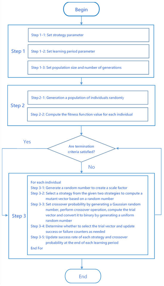
Figure 1.
A flowchart of a two-head self-adaptive algorithm with two strategies.
The overall operation of the proposed algorithm is divided into three steps: Step 1: initialization of parameters, Step 2: initialization of the population and Step 3: evolution of the population. In Step 1, the following parameters are initialized: the mutation strategy parameters and , the probability related to generating a scale factor and selecting a mutation strategy, , the crossover probability, , the learning period parameters, , the population size parameter, , and the number of generations, , of the evolution processes. In Step 2, the initial population is created randomly. In Step 3, the individuals in the population evolve through the generation of scale factors, calculation of mutant vectors, calculation of trial vectors, selection of trial vectors and updating the success counter, the failure counter, success rate and related parameters.
After setting the above parameters, the algorithm proceeds to Step 2 to initialize the population and compute the fitness function value of each individual in the population. Then the algorithm executes the main nested loops in Step 3 to evolve the solutions. In Step 3-1, the algorithm calculates the scale factor by generating a random number to determine the probability distribution used to generate the scale factor. If the random number is less than , the scale factor is generated based on a Gaussian distribution. Otherwise, the scale factor is generated based on a uniform distribution. In Step 3-2, the algorithm calculates the mutant vector based on a random number generated from a uniform distribution to determine the mutation strategy to be used. If the random number is less than , the mutation strategy will be used to compute the mutant vector. Otherwise, the mutation strategy will be used to calculate the mutant vector. In Step 3-3, the algorithm calculates the trial vector based on a random number generated from a uniform distribution and the crossover probability, . If the random number is less than , the algorithm sets the value of the element of the trial vector to the value of the corresponding element of the mutant vector. Otherwise, the algorithm sets the value of the element of the trial vector to the value of the corresponding element of the individual. In Step 3-4, the algorithm determines whether to select the trial vector. Step 3-4 also updates the success counter and the failure counter as needed. In Step 3-5, the algorithm updates the success rate, , and at the end of each learning period.
The algorithm updates the crossover probability by the average of the historical crossover probability value of that has successfully improved performance. The historical crossover probability value of that has successfully improved performance is stored in a list in Step 3-4. Therefore, the crossover probability is updated by .
The algorithm will exit if the termination condition is satisfied. The pseudo code of a two-head self-adaptive metaheuristic algorithm with two DE mutation strategies is shown in Algorithm 1.
| Algorithm 1: Discrete Two-head Self-Adaptive Metaheuristic Algorithm |
| Step 1: Set parameters Step 1-2: Set learning period = 0.5 Step 1-3: Set population size and the number of generations Step 2: Generate a population randomly and evaluate fitness function values of individuals in the population Step 2-1: individuals randomly in the population Step 2-2: Compute each individual’s fitness function value Step 3: Improve solutions through evolution Step 3-1: Create a random number Step 3-2: Create a random number 1, 2, ..., is defined in Table 3. End For Step 3-3: 1, 2, ..., Create a uniform random number End For Step 3-4: Update the success counter or failure counter Else End If End For Step 3-5: End If End For |
5. Results
The goal of this study is to validate whether the old saying “Two heads are better than one” holds for the two-head self-adaptive differential evolution algorithms created to solve the DGRP. That is, each two-head self-adaptive differential evolution algorithm is better than the corresponding two single-head differential evolution algorithms for solving the DGRP. In this study, it is assumed that the two distinct strategies used to create a two-head self-adaptive differential evolution algorithm are arbitrarily selected from the four DE mutation strategies defined in Table 3. Therefore, we can generate 6(=4!/(2!2!) two-head self-adaptive metaheuristic algorithms. A series of experiments were designed to validate the aforementioned statement that the above saying holds for the two-head self-adaptive differential evolution algorithms created to solve the DGRP.
To describe the experiments conducted in this study, let = {1,2,3,4} denote the set of four mutation strategies defined in Table 3. Let us refer to the two-head self-adaptive metaheuristic algorithm created based on strategies and as , where , and . To validate that the above saying holds, we must show that the performance of is better than those of and . We conducted the experiments by applying , and to solve the same set of test cases. Table 4 lists all the experiments conducted in this study. In the first experiment, we compared with and . In the second experiment, we compared with and . In the third experiment, we compared with and . Similarly, we compared with and in the fourth experiment and compared with and in the fifth experiment. Finally, we compared with and .
Table 4.
Experiments to Validate “Two Heads Are Better Than One”.
We introduce preparation of the data and the parameters used by the algorithms in the experiments as follows. The data of the test cases used in the experiments were generated randomly in a region in Taiwan. The method to generate data for test cases is general and can be applied to generate test cases for other regions in the world. The locations corresponding to the randomly generated data will be restricted to the specified region. A large region represents a large geographic area whereas a small region represents a small geographic area. Data generated with a large region are suitable for simulating long-distance ride sharing whereas data generated with a small region are suitable for short-distance sharing. The input data of each test case include the itineraries of drivers and the itineraries of passengers. An itinerary of a passenger includes an identification number, the location to pick up the passenger, the location to drop the passenger off, the original transport cost, the number of seats requested, the earliest departure time and the latest arrival time. An itinerary of a driver includes an identification number, the start location of the driver, the destination location of the driver, the earliest departure time and the latest arrival time. The bids of drivers and the bids of passengers were generated by applying the Bid Generation Algorithm for Drivers and the Bid Generation Procedure for Passengers in [5].
By applying the above procedures, several test cases were generated and used in each series of experiments. Case 1 through Case 10 are small test cases whereas Case 11 through Case 14 are larger test cases. These test cases are available for download via the links in [40]. The format of each file is also defined in a text file accessible via the link. The parameters used in and and for Case 1 through Case 10 are different from the ones for Case 11 through Case 14.
The design of the test cases generated in [40] is based on the approach of incremental tests described in the report “Evaluation Criteria for the CEC 2017 Competition and Special Session on Constrained Single Objective Real-Parameter Optimization” published in [41], which states that four instances (problems with dimensions 10, 30, 50 and 100) of each constrained optimization problem must be solved by an algorithm to test its performance. Although the DGRP is different from the 28 constrained optimization problems in the CEC 2017 Competition and the decision variables are discrete values instead of real values, the way to test the performance of an algorithm for solving the DGRP can also be developed based on the incremental tests used in the CEC 2017 Competition. In this study, the problem dimensions of the 14 test cases for the DGRP are increased from 14 to 100. The dimensions of the 14 test cases in this study are 14, 16, 17, 18, 20, 22, 24, 26, 28, 30, 40, 60, 80 and 100. Therefore, the method to evaluate the algorithms included in this study is similar to the one adopted in the CEC 2017 Competition for Large-Scale Global Optimization (LSGO) and covers more instances of the DGRP with various dimensions than the four instances specified in the LSGO report.
For the parameters used by the algorithms in the experiments, each algorithm needs a number of algorithmic parameters to work properly. Some of the algorithmic parameters are common to all the algorithms related to this study whereas other parameters are specific to a particular algorithm. The values of the algorithmic parameters used by each algorithm in the experiments are listed in Table 5.
Table 5.
Parameters used in the algorithms , , and .
Based on the parameters described above, we ran each algorithm ten times. The results of Experiment 1 obtained by applying the two-head self-adaptive algorithm , and to the test cases are summarized in Table 6. Figure 2 shows the results in a bar chart. The results show that the performance of is either better than or the same as and . Note that the performance of is either better than or the same as for all test cases. In particular, significantly outperforms and for larger cases, Case 12, Case 13 and Case 14. The results show that the saying is valid for .
Table 6.
The results (average fitness values and average number of generations) obtained by applying , and to the test cases.
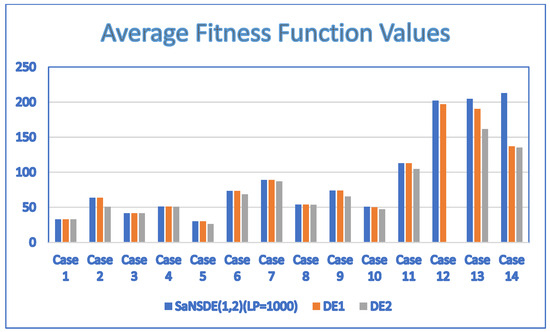
Figure 2.
Comparison of , and .
The results of Experiment 2 obtained by applying the two-head self-adaptive algorithm , and to the test cases are summarized in Table 7. Figure 3 shows the results in a bar chart. The results show that the performance of is either better than or the same as that of . The results show that the performance of is either better than or the same as that of . In particular, significantly outperforms and for larger cases, Case 12, Case 13 and Case 14. The results show that the saying is valid for .
Table 7.
The results (average fitness values and average number of generations) obtained by applying , and to the test cases.
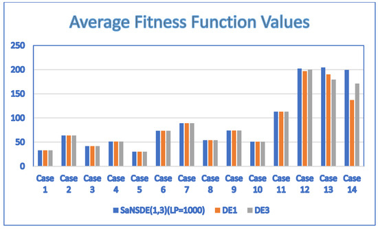
Figure 3.
Comparison of with and .
The results of Experiment 3 obtained by applying the two-head self-adaptive algorithm , and to the test cases are summarized in Table 8. Figure 4 shows the results in a bar chart. The results show that the performance of is either better than or the same as that of . The results show that the performance of is either better than or the same as that of . In particular, significantly outperforms and for larger cases, Case 12, Case 13 and Case 14. The results show that the saying is valid for .
Table 8.
The results (average fitness values and average number of generations) obtained by applying , and to the test cases.
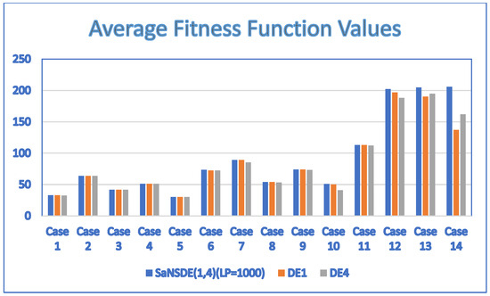
Figure 4.
Comparison of with and .
The results of Experiment 4 obtained by applying the two-head self-adaptive algorithm , and to the test cases are summarized in Table 9. Figure 5 shows the results in a bar chart. The results show that the performance of is either better than or the same as that of . The results show that the performance of is either better than or the same as that of . In particular, significantly outperforms and for larger cases, Case 12, Case 13 and Case 14. The results show that the saying is valid for .
Table 9.
The results (average fitness values and average number of generations) obtained by applying , and to the test cases.
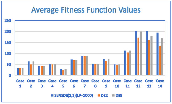
Figure 5.
Comparison of with and .
The results of Experiment 5 obtained by applying the two-head self-adaptive algorithm , and to the test cases are summarized in Table 10. Figure 6 shows the results in a bar chart. The results show that the performance of is either better than or the same as that of . The results show that the performance of is either better than or the same as that of . In particular, significantly outperforms and for larger cases, Case 12, Case 13 and Case 14. The results show that the saying is valid for .
Table 10.
The results (average fitness values and average number of generations) obtained by applying , and to the test cases.
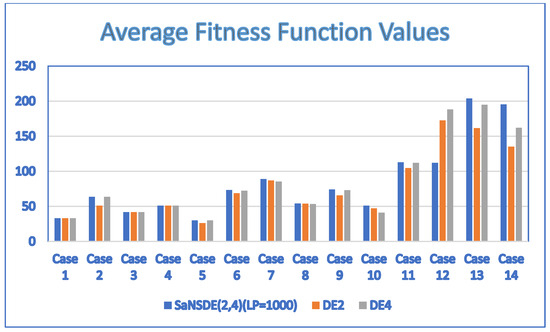
Figure 6.
Comparison of with and .
The results of Experiment 6 obtained by applying the two-head self-adaptive algorithm , and to the test cases are summarized in Table 11. Figure 7 shows the results in a bar chart. The results show that the performance of is either better than or the same as that of . The results show that the performance of is either better than or the same as that of . In particular, significantly outperforms and for larger cases, Case 12, Case 13 and Case 14. The results show that the saying is valid for .
Table 11.
The results (average fitness values and average number of generations) obtained by applying , and to the test cases.
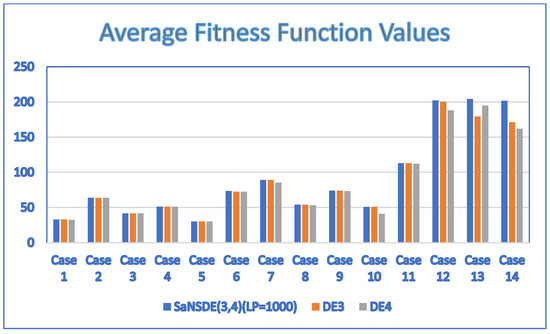
Figure 7.
Comparison of with and .
Table 12 shows the average fitness values and average number of generations for , , , , and . Figure 8 shows the results in a bar chart. Note that these two-head algorithms generate the same average fitness values for all test cases with the exception of Case 13 and Case 14.
Table 12.
Average fitness values and average number of generations for , , , , and .
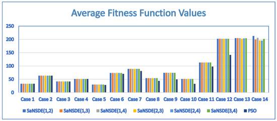
Figure 8.
Comparison of , , , , , and .
In addition to comparing the two-head self-adaptive algorithms with the single-head DE algorithms, we also compared the two-head self-adaptive algorithms with the algorithm. The results obtained by are shown in Table 12 for comparing , , , , , with . The results show that , , , , , outperform in terms of average fitness values for test Case 3 through test Case 14 and the average fitness values for test Case 1 and test Case 2 are the same for all of these algorithms. For convergence speed, , , , , , outperform in terms of the average number of generations for test Case 1 through test Case 12 and test Case 14. The only exception is test Case 13. For test Case 13, , , , outperform in terms of the average number of generations. The average numbers of generations of and are greater than that of for test CASE 13. In spite of these exceptions, , , , , , outperform in terms of the average number of generations for most test cases.
In this paper, we apply the standard deviation to study the robustness property of the two-head self-adaptive algorithms. The standard deviation is used to measure the amount of variation of the average fitness values. The standard deviation presented in this paper is the same as the one defined in statistics. It can be calculated using Excel. Suppose there are observations or outputs , , , …., obtained by experiments. The standard deviation is calculated by the formula , where is the mean of , , , …., . In this study, the outputs of experiments, , , , …., , in the above formula are the average fitness values of experiments for all test cases.
To study the robustness property of the two-head self-adaptive algorithms, we calculated the average fitness value, standard deviation of average fitness values and normalized standard deviations of average fitness values of , , , , , . The results are shown in the three columns on the left in Table 13. It indicates that the normalized standard deviation of average fitness values of all of these two-head self-adaptive algorithms is zero for Case 1 through Case 12 and is very small for Case 13 and Case 14.
Table 13.
Average fitness value, standard deviation and normalized standard deviation of average fitness value of all , where , and all , where .
To compare the robustness property of the two-head self-adaptive algorithms with , , and , we also calculate the average fitness value, standard deviation of average fitness values and normalized standard deviation of average fitness values of , , and . The results are shown in the three columns on the right in Table 13. The results indicate that the normalized standard deviations of average fitness values of all of these single-head DE algorithms are significantly larger than those of the two-head algorithms for all cases. In summary, the two-head self-adaptive algorithms are more robust than the single-head DE algorithms.
We also compared the robustness property of the two-head self-adaptive algorithms with the algorithm. The results are shown in Table 14. It indicates that the normalized standard deviation of the algorithm is significantly larger than those of the two-head algorithms for all cases. In summary, the two-head self-adaptive algorithms are more robust than the algorithm.
Table 14.
Comparison of normalized standard deviation of all , where , and .
6. Discussion
With its long history, the saying “Two heads are better than one” has been widely used in daily life to encourage two people to work together to solve a problem and obtain a better solution rather than working alone. However, the application of this saying in creating new optimization algorithms is still limited. Although the old saying works effectively for human beings to solve problems, whether it can also work for developers to create effective optimization problem solvers in the realm of artificial intelligence is an interesting research question. In this study, we have validated the effectiveness of creating new self-adaptive algorithms based on this old saying to solve the DGRP. In our previous study, one self-adaptive algorithm was proposed to solve the DGRP. In this study, we have demonstrated how to create a series of self-adaptive algorithms based on the old saying and validate the effectiveness of this approach based on experiments and comparison with the algorithms proposed previously. We created two-head self-adaptive algorithms, each with two mutation strategies arbitrarily selected from a set of four mutation strategies. Six self-adaptive algorithms were created. To validate whether the old saying holds for the six two-head self-adaptive algorithms created, we applied each of the six two-head self-adaptive algorithms and also the corresponding two single-head algorithms to solve several test cases. Then we compared the results of experiments.
Due to the additional constraints in the DGRP, the computational complexity of the problem addressed in this paper is at least NP-hard. There is no known efficient method to find the optimal solution for NP-hard problems. Evolutionary algorithms are widely used to find approximate solutions for NP-hard problems. Scalability is an important property that determines whether an algorithm can solve a problem effectively as the scale of the problem grows. A scalable algorithm works effectively as the problem dimension (or the number of decision variables) is increased significantly. For the results in Table 12, performance of the algorithm deteriates seriously for test Case 8 through test Case 14 whereas the two-headed algorithms , , , , , work effectively for all test cases. This shows that the two-headed algorithms , , , , , are more scalable in comparison with .
Although the performance of each two-head SaNSDE algorithm is either the same as or better than that of the corresponding two single-head DE algorithms for smaller cases, each two-head SaNSDE algorithm outperforms the corresponding two single-head DE algorithms for bigger cases. For example, significantly outperforms and for larger cases, Case 12, Case 13 and Case 14. This shows that a two-head SaNSDE algorithm is more scalable than the corresponding two single-head DE algorithms. Thus, the two-head SaNSDE algorithms created based on the proposed method improve scalability. The results indicated that each two-head self-adaptive algorithm outperforms the corresponding two single-head algorithms. By calculating the normalized standard deviation of average fitness values of all two-head self-adaptive algorithms and the single-head algorithms in solving the test cases, it is indicated that the normalized standard deviation of average fitness values of all of these single-head DE algorithms is significantly larger than that of the two-head algorithms for all cases. Based on these results, a new finding is that the two-head self-adaptive algorithms are more robust than the single-head DE algorithms. Another finding of this study is that the old saying not only works effectively for human beings to solve problems but also works effectively in the creation of new self-adaptive algorithms to solve the DGRP. In other words, the effectiveness of applying the old saying can be transferred from solving a problem for human beings to solving an optimization problem in the realm of artificial intelligence. The old saying provides a simple and systematic approach to the development of effective optimization problem solvers in artificial intelligence.
Although the results presented in this study show that the two-head self-adaptive algorithms are more scalable than the corresponding standard DE algorithms and the standard PSO algorithm for the DGRP with dimensions no greater than 100, finding the largest dimension of the DGRP instance that can be solved effectively by the two-head self-adaptive algorithms requires further study and is an interesting future research directions as it is non-trivial. To the best of our knowledge, there is no “one size fits all” evolutionary algorithm that is able to effectively solve a problem of arbitrary size. When an evolutionary algorithm cannot work effectively for a large problem, several mechanisms such as problem decomposition and sub-populations [41] can be applied to improve the scalability of the evolutionary algorithm. Combining such mechanisms with the two-head self-adaptive algorithms developed in this paper is non-trivial and is an interesting future research direction to further increase the scalability of the two-head self-adaptive algorithms developed in this paper.
7. Conclusions
Ridesharing is one popular transport mode to enhance the sustainability of cities. To incentivize drivers and riders to accept ridesharing through the guarantee of a discount, the DGRP has been formulated. Due to computational complexity issues, metaheuristic algorithms can be developed to solve the DGRP. Metaheuristic algorithms have been widely used in many fields such as management, engineering, operation research, transportation and design due to their ability to solve complex optimization problems that cannot be solved by classical optimization methods. For problems in which the gradient of the objective function cannot be obtained, metaheuristic algorithms can still be applied. Therefore, metaheuristic algorithms are not problem specific and can be applied to solve problems in a variety of domains without restriction. Metaheuristic algorithms are typical stochastic optimization algorithms that create candidate trial solutions iteratively based on the candidate solutions found previously to improve the solution quality. Although there is no guarantee that the global optimum of a problem can always be found by applying metaheuristic algorithms, metaheuristic algorithms usually produce quality solutions that are useful in practice. Due to the advantages mentioned above, a lot of metaheuristic algorithms have been proposed to solve complex optimization problems in different problem domains. In the literature, metaheuristic algorithms were created in different ways based on ideas from physics, the concept of swarms in natural or artificial systems, the phenomena of biological evolution, simulating the behavior of different entities in games and with inspiration from human activities or human intelligence such as sayings or proverbs. In this paper, we focused on validation of the effectiveness of creating new self-adaptive differential evolution algorithms based on the old saying “Two heads are better than one” to solve the DGRP.
Each new self-adaptive differential evolution algorithm developed in this paper is a two-head self-adaptive algorithm created based on selecting two different mutation strategies from a set of four mutation strategies. A total of six two-head self-adaptive algorithms were created. To validate whether the old saying holds for the six self-adaptive algorithms created, we compared the results obtained by applying each of the six two-head self-adaptive algorithms with the corresponding two single-head algorithms and PSO algorithm to solve several test cases. The results indicate that each two-head self-adaptive algorithm outperforms the corresponding two single-head algorithms and PSO algorithm in solving most test cases. One new finding is that the two-head self-adaptive algorithms created based on the saying are more scalable and robust than the corresponding single-head DE algorithms and algorithm for problem instances with a number of decision variables no greater than 100, the problem size used in the CEC 2017 Competition for Large-Scale Global Optimization (LSGO). Another finding of this study is that the old saying that works effectively for human beings to solve problems also works effectively in the creation of new self-adaptive algorithms to solve the DGRP. In one of our previous papers, we demonstrated the validity of applying the saying “Two heads are better than one” to develop two-head self-adaptive algorithms to solve another instance of the ridesharing problem for trust-based shared mobility systems. The results of our previous paper and current paper are encouraging as we have demonstrated that applying the above saying to develop two-head self-adaptive algorithms to solve the ridesharing problem in trust-based shared mobility systems and the DGRP is effective. The results of this study have limitations. The strategies used in this study are mutation strategies in DE. Whether the results still hold for strategies of different metaheuristic algorithms requires further study. Although the two-head self-adaptive algorithms created in this study can work effectively for instances of problems with dimensions no greater than 100, finding the largest DGRP instance that can be solved effectively by the two-head self-adaptive algorithms and developing a method to increase the scalability of the proposed algorithms to tackle larger instances of the DGRP are challenging future research directions. Another future research direction is to study whether the way to develop two-head self-adaptive algorithms in this study is effective for other problems. Although the two-headed algorithms are proposed for single-objective optimization problems, they can be applied to solve multi-objective optimization problems based on the weighted sum method for multi-objective optimization. The other interesting future research direction is to study the effectiveness of applying the two-headed algorithms to ridesharing problems with multi-objective functions.
Funding
This research was supported in part by the National Science and Technology Council, Taiwan, under Grant NSTC 111-2410-H-324-003.
Institutional Review Board Statement
Not applicable.
Informed Consent Statement
Not applicable.
Data Availability Statement
The original data presented in the study are available in https://drive.google.com/drive/folders/1COGSGVgo9bjjqpUdY29bxptyO6LlzXKd?usp=sharing.
Conflicts of Interest
The author declares no conflicts of interest.
References
- Uber. Available online: https://www.uber.com (accessed on 29 November 2023).
- Lyft. Available online: https://www.lyft.com (accessed on 29 November 2023).
- Agatz, N.; Erera, A.; Savelsbergh, M.; Wang, X. Optimization for dynamic ride-sharing: A review. Eur. J. Oper. Res. 2012, 223, 295–303. [Google Scholar] [CrossRef]
- Furuhata, M.; Dessouky, M.; Ordóñez, F.; Brunet, M.; Wang, X.; Koenig, S. Ridesharing: The state-of-the-art and future direc-tions. Transp. Res. Part B Methodol. 2013, 57, 28–46. [Google Scholar] [CrossRef]
- Hsieh, F.-S.; Zhan, F.; Guo, Y. A solution methodology for carpooling systems based on double auctions and cooperative coevolutionary particle swarms. Appl. Intell. 2019, 49, 741–763. [Google Scholar] [CrossRef]
- Jin, Q.; Li, B.; Cheng, Y.; Zhao, X. Real-time Multi-platform Route Planning in ridesharing. Expert Syst. Appl. 2024, 255, 124819. [Google Scholar] [CrossRef]
- Nitter, J.; Yang, S.; Fagerholt, K.; Ormevik, A.B. The static ridesharing routing problem with flexible locations: A Norwegian case study. Comput. Oper. Res. 2024, 167, 106669. [Google Scholar] [CrossRef]
- Li, W.; Yu, T.; Zhang, Y.; Chen, X. A shared ride matching approach to low-carbon and electrified ridesplitting. J. Clean. Prod. 2024, 467, 143031. [Google Scholar] [CrossRef]
- Mourad, A.; Puchinger, J.; Chu, C. A survey of models and algorithms for optimizing shared mobility. Transp. Res. Part B Methodol. 2019, 123, 323–346. [Google Scholar] [CrossRef]
- Martins, L.C.; Torre, R.; Corlu, C.G.; Juan, A.A.; Masmoudi, M.A. Optimizing ride-sharing operations in smart sustainable cities: Challenges and the need for agile algorithms. Comput. Ind. Eng. 2021, 153, 107080. [Google Scholar] [CrossRef]
- Ting, K.H.; Lee, L.S.; Pickl, S.; Seow, H.-V. Shared Mobility Problems: A Systematic Review on Types, Variants, Characteristics, and Solution Approaches. Appl. Sci. 2021, 11, 7996. [Google Scholar] [CrossRef]
- Hu, S.; Dessouky, M.M.; Uhan, N.A.; Vayanos, P. Cost-sharing mechanism design for ride-sharing. Transp. Res. Part B Methodol. 2021, 150, 410–434. [Google Scholar] [CrossRef]
- Jiao, G.; Ramezani, M. Incentivizing shared rides in e-hailing markets: Dynamic discounting. Transp. Res. Part C Emerg. Technol. 2022, 144, 103879. [Google Scholar] [CrossRef]
- Hsieh, F.-S. A Comparison of Three Ridesharing Cost Savings Allocation Schemes Based on the Number of Acceptable Shared Rides. Energies 2021, 14, 6931. [Google Scholar] [CrossRef]
- Hsieh, F.-S. Improving Acceptability of Cost Savings Allocation in Ridesharing Systems Based on Analysis of Proportional Methods. Systems 2023, 11, 187. [Google Scholar] [CrossRef]
- Hsieh, F.-S. A Self-Adaptive Meta-Heuristic Algorithm Based on Success Rate and Differential Evolution for Improving the Performance of Ridesharing Systems with a Discount Guarantee. Algorithms 2024, 17, 9. [Google Scholar] [CrossRef]
- Dehghani, M.; Trojovská, E.; Trojovský, P. A new human-based metaheuristic algorithm for solving optimization problems on the base of simulation of driving training process. Sci. Rep. 2022, 12, 9924. [Google Scholar] [CrossRef]
- Guilmeau, T.; Chouzenoux, E.; Elvira, V. Simulated Annealing: A Review and a New Scheme. In Proceedings of the 2021 IEEE Statistical Signal Processing Workshop (SSP), Rio de Janeiro, Brazil, 11–14 July 2021; pp. 101–105. [Google Scholar] [CrossRef]
- Rashedi, E.; Nezamabadi-pour, H.; Saryazdi, S. GSA: A Gravitational Search Algorithm. Inf. Sci. 2009, 179, 2232–2248. [Google Scholar] [CrossRef]
- Eberhart, R.C.; Shi, Y. Comparison between genetic algorithms and particle swarm optimization. In Lecture Notes in Computer Science; Springer: Berlin/Heidelberg, Germany, 1998; Volume 1447, pp. 611–616. [Google Scholar]
- Yang, X.S. Firefly algorithms for multimodal optimization. In Lecture Notes in Computer Science; Springer: Berlin/Heidelberg, Germany, 2009; Volume 5792, pp. 169–178. [Google Scholar]
- Karaboga, D.; Basturk, B. Artificial Bee Colony (ABC) Optimization Algorithm for Solving Constrained Optimization Problems. In Lecture Notes in Computer Science; Melin, P., Castillo, O., Aguilar, L.T., Kacprzyk, J., Pedrycz, W., Eds.; Foundations of Fuzzy Logic and Soft Computing (IFSA): Cancun, Mexico, 2007; Volume 4529, pp. 789–798. [Google Scholar]
- Dorigo, M.; Birattari, M.; Stutzle, T. Ant colony optimization. IEEE Comput. Intell. Mag. 2006, 1, 28–39. [Google Scholar] [CrossRef]
- Holland, J.H. Adaptation in Natural and Artificial Systems; MIT Press: Cambridge, MA, USA, 1992. [Google Scholar]
- Storn, R.; Price, K. Differential evolution—A simple and efficient heuristic for global optimization over continuous spaces. J. Glob. Optim. 1997, 11, 341–359. [Google Scholar] [CrossRef]
- Dehghani, M.; Mardaneh, M.; Guerrero, J.M.; Malik, O.; Kumar, V. Football game based optimization: An application to solve energy commitment problem. Int. J. Intell. Eng. Syst. 2020, 13, 514–523. [Google Scholar] [CrossRef]
- Moghdani, R.; Salimifard, K. Volleyball premier league algorithm. Appl. Soft Comput. 2018, 64, 161–185. [Google Scholar] [CrossRef]
- Rao, R.V.; Savsani, V.J.; Vakharia, D. Teaching-learning-based optimization: A novel method for constrained mechanical design optimization problems. Comput. Aided Des. 2011, 43, 469–492. [Google Scholar] [CrossRef]
- Moosavi, S.H.S.; Bardsiri, V.K. Poor and rich optimization algorithm: A new human-based and multi populations algorithm. Eng. Appl. Artif. Intell. 2019, 86, 165–181. [Google Scholar] [CrossRef]
- Mousavirad, S.J.; Ebrahimpour-Komleh, H. Human mental search: A new population-based metaheuristic optimization algorithm. Appl. Intell. 2017, 47, 850–887. [Google Scholar] [CrossRef]
- Su, H.; Chen, R.; Tang, S.; Zheng, X.; Li, J.; Yin, Z.; Ouyang, W.; Dong, N. Two Heads Are Better Than One: A Multi-Agent System Has the Potential to Improve Scientific Idea Generation. arXiv 2024, arXiv:2410.09403. [Google Scholar]
- Yuan, L.; Zhang, Z.; Li, L.; Guan, C.; Yu, Y. A Survey of Progress on Cooperative Multi-Agent Reinforcement Learning in Open Environment. arXiv 2023, arXiv:2312.01058. [Google Scholar] [CrossRef]
- Dyba, T.; Arisholm, E.; Sjoberg, D.; Hannay, J.; Shull, F. Are Two Heads Better than One? On the Effectiveness of Pair Programming. IEEE Softw. 2007, 24, 12–15. [Google Scholar] [CrossRef]
- Li, Z.; Xie, L.; Song, H. Two heads are better than one: Dual systems obtain better performance in facial comparison. Forensic Sci. Int. 2023, 353, 111879. [Google Scholar] [CrossRef]
- Jindal, S.; Sparks, A. Synergy at work: Two heads are better than one. J. Assist. Reprod. Genet. 2018, 35, 1227–1228. [Google Scholar] [CrossRef]
- Li, A.; Liu, W.; Zheng, C.; Fan, C.; Li, X. Two Heads are Better Than One: A Two-Stage Complex Spectral Mapping Approach for Monaural Speech Enhancement. IEEE/ACM Trans. Audio Speech Lang. Process. 2021, 29, 1829–1843. [Google Scholar] [CrossRef]
- Hsieh, F.-S. Comparison of a Hybrid Firefly–Particle Swarm Optimization Algorithm with Six Hybrid Firefly–Differential Evolution Algorithms and an Effective Cost-Saving Allocation Method for Ridesharing Recommendation Systems. Electronics 2024, 13, 324. [Google Scholar] [CrossRef]
- Hsieh, F.-S. Applying “Two Heads Are Better Than One” Human Intelligence to Develop Self-Adaptive Algorithms for Ridesharing Recommendation Systems. Electronics 2024, 13, 2241. [Google Scholar] [CrossRef]
- Deb, K. An efficient constraint handling method for genetic algorithms. Comput. Methods Appl. Mech. Eng. 2000, 186, 311–338. [Google Scholar] [CrossRef]
- Data of Test Cases 1–14. Available online: https://drive.google.com/drive/folders/1COGSGVgo9bjjqpUdY29bxptyO6LlzXKd?usp=sharing (accessed on 26 February 2025).
- Wu, G.; Mallipeddi, R.; Suganthan, P.N. Problem Definitions and Evaluation Criteria for the CEC 2017 Competition and Special Session on Constrained Single Objective Real-Parameter Optimization, Technical Report, 2016. Available online: https://www.researchgate.net/publication/317228117_Problem_Definitions_and_Evaluation_Criteria_for_the_CEC_2017_Competition_and_Special_Session_on_Constrained_Single_Objective_Real-Parameter_Optimization#fullTextFileContent (accessed on 7 March 2025).
Disclaimer/Publisher’s Note: The statements, opinions and data contained in all publications are solely those of the individual author(s) and contributor(s) and not of MDPI and/or the editor(s). MDPI and/or the editor(s) disclaim responsibility for any injury to people or property resulting from any ideas, methods, instructions or products referred to in the content. |
© 2025 by the author. Licensee MDPI, Basel, Switzerland. This article is an open access article distributed under the terms and conditions of the Creative Commons Attribution (CC BY) license (https://creativecommons.org/licenses/by/4.0/).