Modeling and Experimental Investigation of the Evolution of Surface Temperature Fields in Water Bodies

Abstract

The variation in the background temperature field in aquatic environments plays a crucial role in the detection of thermal signatures of maritime moving targets. To elucidate the influence of various meteorological and hydrological parameters on the background temperature field of water bodies, this study employs the COARE 3.0 model to analyze the relationship between the net heat flux at the air–water interface and the characteristics of the cool skin layer. By examining the diurnal fluctuations of environmental parameters, the diurnal variation patterns of the cool skin layer properties are investigated. A dynamic temperature field testing platform was established in an outdoor pool to measure air–water volume variables and validate the accuracy of the water temperature field calculation model. The findings indicate that the cool skin phenomenon is indeed present in natural aquatic environments. The properties of the cool skin layer are predominantly affected by factors such as wind speed, the specific humidity gradient between the near-surface and high-altitude regions, and the temperature gradient between these regions. The temperature of the cool skin layer is typically a few tenths of K lower than that of the subsurface water, with a thickness generally ranging from 2 to 5 mm.

1. Introduction

Water temperature is a vital parameter that reflects the state of aquatic systems. Understanding sea surface temperature (SST) is crucial for investigating meteorological variations, fish growth dynamics, underwater acoustic propagation, and infrared detection of maritime targets [1]. SST is a fundamental physical parameter at the air–sea interface, frequently utilized as a boundary condition to estimate heat exchange between the ocean and atmosphere, as well as freshwater exchange driven by precipitation and evaporation. Consequently, high-precision and high spatial-resolution SST data are indispensable for accurate weather forecasting and effective climate change monitoring [2]. Furthermore, the sea surface acts as a significant background for military targets, with its infrared radiation characteristics forming the foundation for infrared guidance systems in maritime operations. The infrared radiation signatures of ship wakes, generated through the interaction between ship wakes and sea surface temperature, represent a critical target source for infrared detection systems [3,4].

Since the 20th century, many maritime nations have conducted extensive research on sea surface and subsurface seawater temperatures. The development of satellite and aerial remote sensing, along with deep-water exploration technologies, has significantly advanced the analysis and forecasting of seawater temperatures in offshore and oceanic areas, which has fostered substantial scientific progress [5,6]. In the study of sea surface temperature, researchers primarily utilize regression-based statistical models, deterministic models, machine learning models, and hybrid models for modeling. These approaches, each with distinct advantages, contribute to a comprehensive understanding of sea surface temperature dynamics, enriching the theoretical foundation of the field [7]. Piccolroaz [8] had developed a physics-based simplified model to estimate surface water temperature from air temperature data, deriving a simplified differential equation. Donlon [9] and Minnett [10] introduced multiple parameterization approaches to estimate the cool skin temperature difference, formulated as a function of the wind speed U₁₀ at 10 m above the surface, thereby building the relationship between wind speed and the cool skin temperature difference. MacCallum [11] introduced an optimal estimation and probabilistic cloud-screening approach for estimating lake surface water temperature. The study found that the daytime satellite in situ difference was −0.2 ± 0.7 K, while the nighttime difference was −0.1 ± 0.5 K. White [12] proposed a machine learning algorithm trained using in situ and multispectral satellite data for extracting sea surface temperature (SST). The method employs Shapley values to assess feature importance and utilizes spectral bands and metadata for prediction, significantly enhancing the accuracy and reliability of SST estimation. Kong [13] utilized Landsat 8 satellite data and applied the radiative transfer equation, single-channel algorithm, and split-window algorithm to retrieve lake surface temperature in the study area. The distribution of water temperature is influenced by numerous factors. Fedorets [14] et al. investigated the surface temperature of levitating water droplets using infrared spectroscopy. In the water absorption band around 3 μm, they established an inverse problem for determining the upper surface temperature by considering the directional spectral emissivity of the droplet surface and the spectral sensitivity of the detector. Guo [15] assessed the simulation algorithms for four critical lake thermal processes—turbulent heat flux, wind-driven mixing, light extinction, and snow density—and analyzed the simulation results. This work offered practical parameterization strategies to enhance the one-dimensional lake thermal model, advancing the understanding of lake thermal dynamics. Fedorets [16] explored the impact of salinity on water temperature fields, noting that when water evaporates, a thin layer with increased salt concentration forms on its surface, preventing further evaporation of the water. Liu [17] pointed out that water constituents (such as phytoplankton) modulate the penetration process of visible solar radiation in the upper ocean and influence the mixing processes and heat transfer within the water column.

Water surface temperature measurement primarily relies on in situ monitoring and satellite observation. In situ monitoring provides high-precision, real-time data through sensor deployment, whereas satellite observation enables continuous, large-scale monitoring using remote sensing technology. Together, these methods offer a robust framework for accurate water surface temperature assessment [18]. With the rise of spatial distribution monitoring, automated vessels and unmanned aerial vehicles (UAVs) are increasingly being used to measure surface water temperature [19]. In situ measurement employs mercury thermometers [20], multi-parameter probes [21], or thermistor-equipped mooring stations [22] to collect water temperature data at discrete depths, either automatically or manually. In situ measurement data are often challenging to obtain and limited in spatial scale and regional coverage. Satellite observations, however, provide a global data source that corrects latitude biases in in situ surface water temperature monitoring. By using satellite-mounted radiometers to measure surface water temperature, this approach resolves the standardization issues of long-term ground-based data and enhances the comprehensiveness and reliability of spatial surface water temperature characterization, opening new avenues for water temperature research [23]. Fu [24] created a climate data record of sea surface temperature under rain-free ocean conditions based on over two decades of data from three satellite instruments. Compared to in situ radiosonde and buoy observations, the satellite-derived SST exhibited a bias of 0.2 K and a root-mean-square error of 1.6 K, demonstrating the precision and reliability of satellite data for ocean temperature monitoring and advancing global SST climate studies. Sharma [25] created a global lake temperature database based on satellite observations of summer lake surface temperatures from 291 lakes, investigating spatial and temporal patterns of water temperature variations globally and regionally. Sima [26] proposed an innovative method for retrieving plateau lake surface temperature (p-LWST) using unmanned aerial vehicle (UAV) thermal infrared (TIR) data. The results demonstrated that the method successfully retrieved LWST in the Erhai region of the plateau, with temperatures ranging from 288 K to 295 K and a final accuracy of 0.89 K. Infrared measurement technology is now extensively applied in oceanography to detect breaking waves, microscale breaking waves, fronts, and internal wave structures [27], and to study the thermal boundary layer and its connection to ocean heat flux. In the context of remote sensing and satellite sea surface temperature measurements, the measurement of the so-called “cool skin” phenomenon has garnered significant attention from researchers [9,28,29]. Prats [30] utilized Landsat 5 and Landsat 7 archived images to create the skin surface temperature dataset, which includes surface water temperature data from 442 French inland water bodies. By comparing satellite temperature measurements with in situ measurements and accounting for the cool skin effect and warm layer effect, the study estimated that the cool skin effect typically ranges between −0.3 °C and −0.6 °C, with the cool skin layer being more frequently observed at night.

This study centers on the thermal signature of wakes produced by the interaction between surface-moving targets and the upper layer of water temperature. From an induction mechanism standpoint, the temperature anomaly region arises from the coupling of the hydrodynamic wake generated by the moving target and the ambient water temperature field. Assuming the intrinsic properties of the moving target—such as its principal dimensions, motion posture, and maneuvering mode—are fixed, the macroscopic state of the hydrodynamic wake can be regarded as relatively stable. However, the ambient water temperature field is temporally dynamic, influenced by a suite of environmental factors including solar radiation, atmospheric humidity, cloud cover, air temperature, and wind speed. Even when the moving target maintains identical motion posture and speed, the characteristic scale, intensity, and decay time of the wake temperature signal can vary significantly across different flight periods and marine meteorological conditions [31,32]. Chen [33] conducted a meticulous investigation into the heat and mass transfer characteristics of stratified wakes generated by underwater vehicles, employing the Large Eddy Simulation (LES) method. The study revealed that these wakes significantly alter the internal temperature and salinity distributions within the water column and produce detectable signatures, providing valuable insights into the hydrodynamic and thermodynamic interactions of underwater vehicles with the surrounding environment. Voropayev [34] discovered that the propellers of surface vessels, during their operation, induce the upward mixing of colder water from several meters below the surface to the upper layers. This process creates a distinct “cold signal” on the water surface, which can be potentially utilized for vessel detection and monitoring purposes. Furthermore, Luo [4] and Wang [35], through systematic experimental investigations, demonstrated that the wakes generated by moving underwater vehicles modulate the surface temperature distribution. This modulation results in the formation of characteristic thermal signatures that are detectable through appropriate sensing technologies. Consequently, fluctuations in the ambient water temperature play a pivotal role in characterizing the wake temperature anomaly signal. Elucidating the variation patterns of background water temperature fields, particularly the temperature distribution characteristics within the surface boundary layer, serves as a crucial prerequisite for investigating the thermal signatures of moving object wakes. A comprehensive exploration of the influence mechanisms of meteorological and hydrological environmental factors (such as wind speed, solar radiation, and precipitation) on the temperature profile structure of water bodies is of paramount importance for achieving effective decoupling between hydrodynamic wakes and background water temperature fields.

This research employs the COARE 3.0 model to compute water–air heat fluxes, enabling the determination of interfacial heat flux. By incorporating the vertical temperature heat balance equation for water bodies, the study derives the vertical temperature distribution and examines the spatiotemporal dynamics of the vertical temperature profile. The analysis extends to the relationship between the net heat flux at the water–air interface and the cold skin properties of the water body. Taking into account the diurnal fluctuations of environmental parameters, the investigation delves into the diurnal variation patterns of the cold skin properties. To validate the accuracy of the water temperature field calculation model, an outdoor pool-based testing platform for dynamic water temperature fields is established, facilitating the measurement of water–air volume variables. This methodology elucidates the impact of various meteorological and hydrological parameter changes on the background environmental temperature field of the water body.

2. Theoretical Model for Water Temperature Field

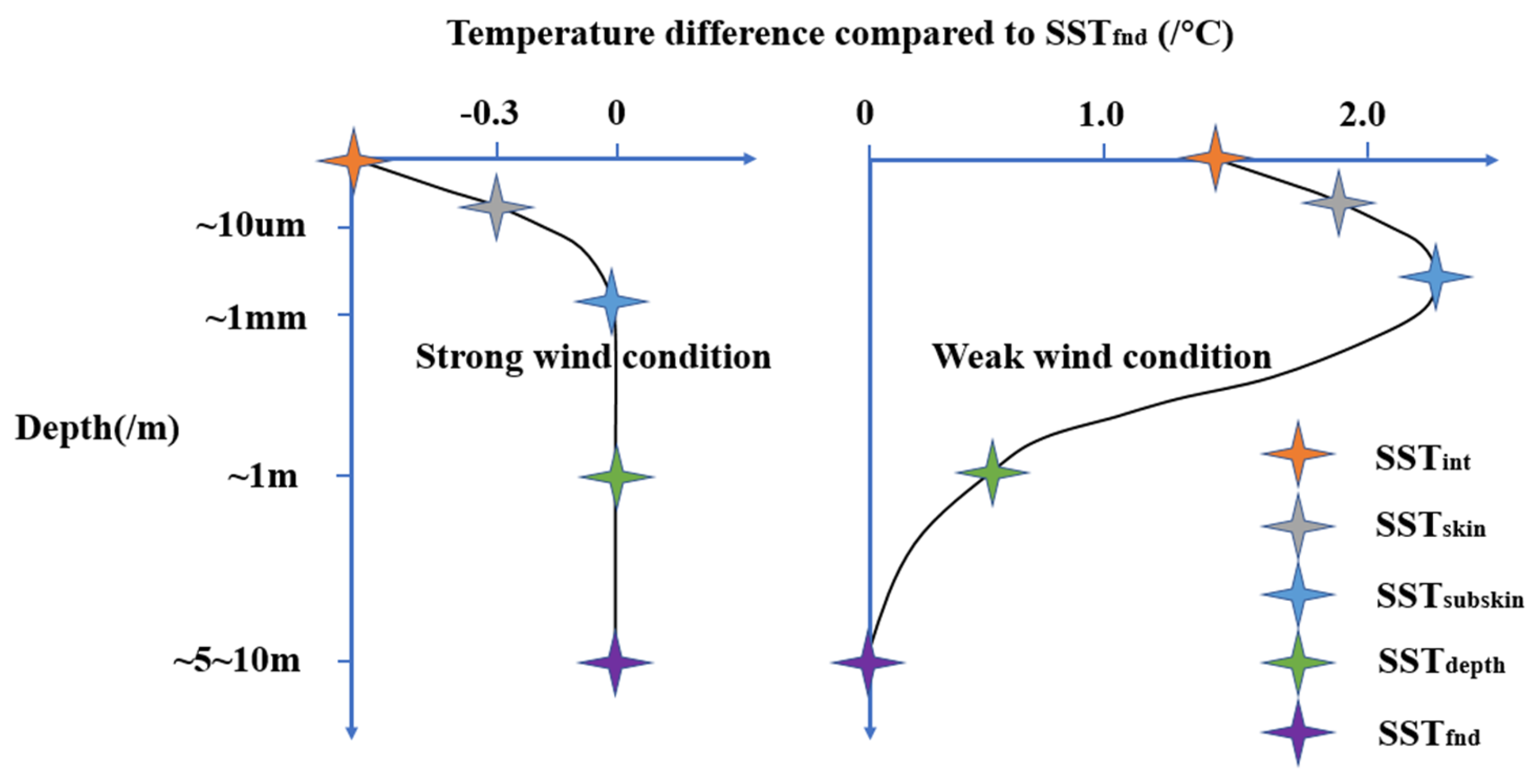
2.1. Vertical Profile Temperature Structure of Water

The scientific team of the Global Ocean Data Assimilation Experiment (GODAE) high-resolution sea temperature test project uses five temperature forms to define the vertical structure of the sea surface temperature [1], as shown in Figure 1. Among them, the water–air interface temperature $SS{T}_{\mathrm{int}}$ represents the temperature of the water at the exact position of the water–air interface in an infinitely thin layer; the skin temperature of the water surface $SS{T}_{skin}$ represents the temperature within a thin layer on the water side of the water–air interface, where there is a strong temperature gradient and diffusive heat transfer dominates; the subsurface skin temperature of the water $SS{T}_{subskin}$ represents the bottom of the temperature gradient layer, where molecular and viscous heat transfer processes dominate. It can be measured by low-frequency microwave radiometers, generally at depths greater than 1 mm; the subsurface temperature of the water $SS{T}_{depth}$, also known as the “bulk” water temperature, refers to the temperature of a layer of water below a certain depth. It is usually located at a specific water depth, for example, $SS{T}_{5m}$ represents the water temperature at a depth of 5 m. It is greatly influenced by solar radiation and varies on an hourly time scale, with convective heat transfer processes dominating. It can be measured by traditional temperature sensors installed on buoys, profilers, and ships; the bottom temperature of the water $SS{T}_{fnd}$ represents the temperature of the water at the maximum depth where solar radiation can reach.

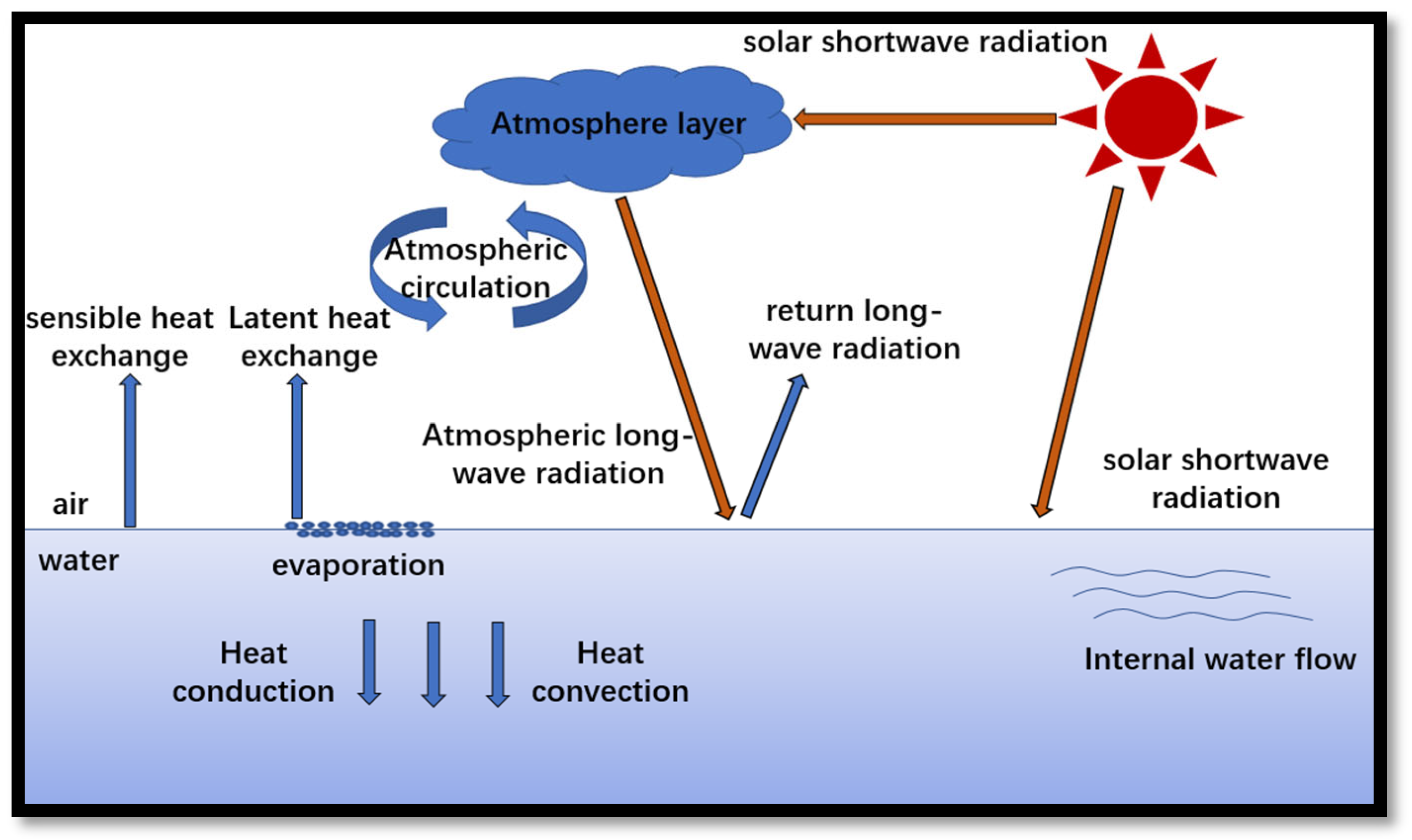
2.2. Gas–Liquid Two-Phase Interface Heat Flux Calculation Model

The primary driver of vertical temperature stratification in water bodies is the heat exchange occurring at the air–water interface. This exchange facilitates a dynamic thermal equilibrium between the water body and the atmosphere through mechanisms such as molecular heat conduction and phase transitions. Within the water body, heat transfer between the upper and lower layers is achieved via heat conduction, convection, and mixing, ultimately establishing stable vertical temperature stratification. As depicted in Figure 2, heat exchange at the air–water interface and within the water body encompasses convective heat transfer, latent heat exchange, and radiative exchange. Radiative exchange includes solar shortwave radiation, atmospheric longwave radiation, and longwave back radiation from the water body. The net heat flux at the air–water interface $\psi$ is expressed as follows [36]:

$$\psi ={\psi }_{nl}+{\psi }_s+{\psi }_l-{\psi }_{ns}$$

(1)

where ${\psi }_s$ represents the sensible heat flux, ${\psi }_l$ denotes the latent heat flux, ${\psi }_{nl}$ is the net longwave radiation flux, calculated as ${\psi }_{nl}={\psi }_{\uparrow l}-{\psi }_{\downarrow l}$ (the difference between atmospheric longwave radiation ${\psi }_{\downarrow l}$ and water body longwave back radiation ${\psi }_{\uparrow l}$), and ${\psi }_{ns}$ signifies the solar shortwave radiation flux absorbed by the interfacial thin layer.

The COARE3.0 (Coupled Ocean-Atmosphere Response Experiment) model is an advanced numerical framework specifically developed to investigate the intricate interactions between the ocean and the atmosphere [37]. This model is predominantly utilized for the precise computation of ocean surface fluxes, including heat, momentum, and moisture fluxes, and is extensively employed in the fields of marine meteorology and climate science. It rigorously implements the Monin–Obukhov similarity theory, a standard approach for near-surface meteorological measurements. Furthermore, the model incorporates sophisticated sub-models to account for the ocean’s cool skin layer and the diurnal warm layer, enhancing its accuracy and applicability in diverse environmental conditions. For specific heat fluxes, the individual components are computed utilizing the air–sea flux model. The sensible heat flux and latent heat flux are mathematically defined as follows [37,38]:

$${\psi }_s={\rho }_a{c}_{pa}\overline{w^{\prime }{T}^{\prime }}=-{\rho }_a{c}_{pa}{u}_{*}{T}_{*}$$

(2)

$${\psi }_l={\rho }_a{L}_e\overline{w^{\prime }{q}^{\prime }}=-{\rho }_a{L}_e{u}_{*}{q}_{*}$$

(3)

where

$$u_{*}=\sqrt{-\tau /{\rho }_a}$$

(4)

where ${\rho }_a$ and $c_{pa}$ denote air density and specific humidity, respectively; $w\prime ,T\prime ,q\prime$ represent the turbulent fluctuations of vertical wind speed, temperature, and water vapor mixing ratio, respectively; $u_{*}$, $T_{*}$, $q_{*}$ are the MOS (Monin–Obukhov Similarity) scaling parameters for velocity, humidity, and temperature, respectively; $L_e$ represents the latent heat of evaporation; and $\tau$ signifies the air shear stress. The standard volumetric expressions for the two fluxes and stress components are as follows:

$${\psi }_s={\rho }_a{c}_{pa}{C}_{h}U(T_{sw}-T_{sa})$$

(5)

$${\psi }_l={\rho }_a{L}_e{C}_{e}U(q_{sa}-q_{ta})$$

(6)

$$\tau ={\rho }_a{C}_{d}U(u_{si}-u_i)$$

(7)

where $C_h$ represents the sensible heat transfer coefficient, $U$ denotes the mean wind speed at height $z_r$ relative to the water surface, $T_{sw}$ is the water surface temperature, and $T_{sa}$ is the air temperature at height $z_r$; $C_e$ signifies the latent heat transfer coefficient, $q_{sa}$ is the specific humidity at the air–water interface, and $q_{ta}$ is the specific humidity at height $z_r$; $C_d$ is the stress transfer coefficient, $u_{si}$ is the water surface velocity, and $u_i$ is the horizontal wind speed component relative to a fixed coordinate system. To determine these transfer coefficients, they are decomposed into relatively independent neutral transfer coefficient components, which are expressed as follows:

$$\begin{array}{l}{C}_h=c_T^{1/2}{c}_d^{1/2}\\ C_e=c_q^{1/2}{c}_d^{1/2}\\ C_d=c_d^{1/2}{c}_d^{1/2}\end{array}$$

(8)

where the neutral transfer coefficients $c_T^{1/2}$, $c_q^{1/2}$, and $c_d^{1/2}$ are reformulated using the flux functions derived from MOS theory, which are expressed as follows:

$$\begin{array}{l}{c}_T^{1/2}=c_{Tn}^{1/2}/[1-{\displaystyle \frac{c_{Tn}^{1/2}}{a_n{f}_k}}{\varphi }_h(\xi )]\\ c_q^{1/2}=c_{qn}^{1/2}/[1-{\displaystyle \frac{c_{qn}^{1/2}}{a_n{f}_k}}{\varphi }_h(\xi )]\\ c_d^{1/2}=c_{dn}^{1/2}/[1-{\displaystyle \frac{c_{dn}^{1/2}}{f_k}}{\varphi }_u(\xi )]\end{array}$$

(9)

where $f_k$ is the von Kármán constant, taken as 0.4 [2]; $a_n$ is the scalar correction factor, taken as 1.0 [38]; and $\xi$ is the MOS stability parameter, satisfying the following equation:

$$\xi =z_r/L$$

(10)

$$L^{-1}={\displaystyle \frac{{\mathrm{f}}_{\mathrm{k}}\mathrm{g}}{T_{sa}}}(T_{*}+0.61T_{sa}{q}_{*})/u_{*}^2$$

(11)

where $L$ is the Obukhov length, $\mathrm{g}$ is the gravitational acceleration, and $\varphi$ is the MOS profile function incorporating the standard Kansas-type model, satisfying the following equation [39]:

$${\varphi }_h={\displaystyle \frac{1}{1+{\xi }^2}}{\varphi }_{hk}+{\displaystyle \frac{{\xi }^2}{1+{\xi }^2}}{\varphi }_c$$

(12)

$${\varphi }_u={\displaystyle \frac{1}{1+{\xi }^2}}{\varphi }_{uk}+{\displaystyle \frac{{\xi }^2}{1+{\xi }^2}}{\varphi }_c$$

(13)

where

$${\varphi }_{hk}=2\ln ({\displaystyle \frac{1+{(1+{\gamma }_1\xi )}^{1/2}}{2}})$$

(14)

$${\varphi }_{uk}=2\ln ({\displaystyle \frac{1+{(1-{\gamma }_2\xi )}^{1/4}}{2}})+2\ln ({\displaystyle \frac{1+{(1-{\gamma }_2\xi )}^{1/2}}{2}})-2\arctan ({(1-{\gamma }_2\xi )}^{1/4})+{\displaystyle \frac{\pi }{2}}$$

(15)

$${\varphi }_c=1.5\ln ({\displaystyle \frac{{(1-{\gamma }_3\xi )}^{2/3}+(1-{\gamma }_3\xi )+1}{3}})-\sqrt{3}\arctan ({\displaystyle \frac{2(1-{\gamma }_3\xi )+1}{\sqrt{3}}})+{\displaystyle \frac{\pi }{\sqrt{3}}}$$

(16)

where ${\gamma }_1$, ${\gamma }_2$, and ${\gamma }_3$ are empirical constants. In Equation (9), the subscript $n$ represents the specific scenario when $\varphi =0$. In this case, the neutral transfer coefficients are directly associated with their corresponding roughness lengths, which are expressed as follows:

$$\begin{array}{l}{c}_{Tn}^{1/2}={\displaystyle \frac{a_n{f}_k}{\log (z_r/z_{oT})}}\\ c_{qn}^{1/2}={\displaystyle \frac{a_n{f}_k}{\log (z_r/z_{oq})}}\\ c_{dn}^{1/2}={\displaystyle \frac{f_k}{\log (z_r/z_o)}}\end{array}$$

(17)

where $z_o$, $z_{o\mathrm{q}}$, and $z_{oT}$ represent the roughness lengths for velocity, humidity, and temperature, respectively. These roughness lengths quantify the strength of heat and moisture transfer via molecular diffusion processes within the thin layer near the water surface. The velocity roughness length satisfies the following equation:

$$z_o=0.011{\displaystyle \frac{u_{*}^2}{g}}+0.11{\displaystyle \frac{v_a}{u_{*}}}$$

(18)

where $v_a$ represents the kinematic viscosity of air. Building on the characteristics of air–water interface interactions, Fairall established the interrelationships and calculation criteria for temperature and humidity roughness parameters, which satisfy the following equation:

$$z_{oq}=z_{oT}=\min (1.15\times {10}^{-4},5.5\times {10}^{-5}\times {({\displaystyle \frac{u_{*}{z}_o}{v_a}})}^{-0.6})$$

(19)

Solar shortwave radiation serves as the primary driver for the formation of thermal stratification in water bodies. The shortwave radiation spectrum is predominantly concentrated in the 0.2–3 μm range, exerting a decisive influence on the thermodynamic and dynamic structure of the upper water layer. Under clear weather conditions, approximately half of the solar radiation energy is absorbed within the upper 2 m of the water body. The region of significant warming propagates downward from the water surface, and wind-driven shear turbulence facilitates the mixing of heat into deeper layers of the water. For optically homogeneous water bodies, the solar radiation absorbed at different water depths ${\psi }_{ns}$ is expressed as follows:

$${\psi }_{ns}(z)={\psi }_{sun}(1-b)\{1-{\displaystyle \frac{1}{z}}{\displaystyle \sum _{i=1}^N{F}_i{\zeta }_i}[1-\exp (-{\displaystyle \frac{z}{{\zeta }_i}})]\}$$

(20)

where ${\psi }_{sun}$ denotes the intensity of solar shortwave radiation, $b$ is the albedo, set to 0.07 [40], $z$ represents the water depth, and $N$ indicates the number of wavelength bands; $F_i$ and ${\zeta }_i$ correspond to the irradiance constant and wavelength irradiance, respectively. Based on the attenuation characteristics of solar spectral bands in water, Simpson [40] discretized the incident solar radiation flux using a 9-wavelength band spectrum. The values of the irradiance constants are provided in

Table 1. Solar irradiance constant at each band.

$\mathit{\lambda }(\mathit{\mu }\mathit{m})$	${\mathit{F}}_{\mathit{i}}$	${\mathit{\zeta }}_{\mathit{i}}(\mathbf{m})$
0.2~0.6	0.237	34.8492
0.6~0.9	0.360	2.2662
0.9~1.2	0.179	3.149 × 10−2
1.2~1.5	0.087	5.483 × 10−3
1.5~1.8	0.080	8.317 × 10−4
1.8~2.1	0.0246	1.261 × 10−4
2.1~2.4	0.025	3.133 × 10−4
2.4~2.7	0.007	7.819 × 10−5
2.7~3.0	0.0004	1.443 × 10−5

.

Before reaching the Earth’s surface, solar radiation is attenuated by the atmosphere. The solar radiation absorbed by the atmosphere is subsequently emitted as longwave radiation in the form of sky background radiation. The intensity of this radiation is influenced by air temperature and cloud cover in the sky, adhering to the Stefan–Boltzmann law:

$${\psi }_{\downarrow l}=\sigma {\epsilon }_a(273.15+T_a)(1-{\gamma }_a)$$

(21)

where $\sigma$ is the Stefan–Boltzmann constant, set as $5.67\times {10}^{-8}W/m^2{K}^4$; ${\gamma }_a$ represents the longwave reflectivity; $T_a$ denotes the air temperature near the water surface; and ${\epsilon }_a$ is the atmospheric emissivity, expressed as follows:

$${\epsilon }_a=1-0.261\exp (-0.74\times {10}^{-4}{T}_a^2)(1+K{C}^2)$$

(22)

where $C$ is the cloud cover fraction, and the parameter $K$ is the cloud height factor, with a mean value of 0.017.

The radiation emitted by the water body back to the atmosphere ${\psi }_{\uparrow l}$ also adheres to the Stefan–Boltzmann law, expressed as follows:

$${\psi }_{\uparrow l}=\sigma {\epsilon }_{\mathrm{w}}{(273.15+T_{sw})}^4$$

(23)

where ${\epsilon }_{\mathrm{w}}$ represents the longwave emissivity of the water body, taken as 0.97.

2.3. Vertical Profile Temperature Calculation Model of Water

When considering the influence of solar radiation, for horizontally homogeneous water bodies, the momentum, temperature, and salinity of any fluid parcel satisfy the following governing equations [41]:

$${\displaystyle \frac{\partial u_x}{\partial t}}=f{u}_y+{\displaystyle \frac{\partial }{\partial z}}[(k_m+v){\displaystyle \frac{\partial u_x}{\partial z}}]$$

(24)

$${\displaystyle \frac{\partial u_x}{\partial t}}=f{u}_y+{\displaystyle \frac{\partial }{\partial z}}[(k_m+v){\displaystyle \frac{\partial u_x}{\partial z}}]$$

(25)

$${\displaystyle \frac{\partial T}{\partial t}}={\displaystyle \frac{\partial }{\partial z}}[(k_t+aa){\displaystyle \frac{\partial T}{\partial t}}]-{\displaystyle \frac{\partial }{\partial z}}({\displaystyle \frac{{\psi }_{ns}}{\rho c_p}})$$

(26)

$${\displaystyle \frac{\partial S}{\partial t}}=-{\displaystyle \frac{\partial }{\partial z}}[(k_s+\gamma ){\displaystyle \frac{\partial S}{\partial z}}]$$

(27)

Among them, $t$ represents time; $u_x$ and $u_y$ denote the velocity components of the fluid parcel along the $x$ and $y$ directions, respectively; $f$ is the Coriolis parameter; $k_m$, $k_t$, and $k_s$ are the eddy diffusion coefficients for momentum, temperature, and salinity, respectively; $v$, $aa$, and $\gamma$ are the molecular diffusion coefficients for momentum, temperature and salinity, respectively; $T$ and $S$ represent the temperature and salinity of the fluid parcel, respectively; $\rho$ is the density of the fluid parcel and $c_p$ is the specific heat of water.

In temperature-stratified water bodies, the formation of the thermocline results in relatively minor horizontal temperature variations. Even under extreme hydrological and wind disturbances, which may temporarily alter longitudinal and transverse gradients, horizontal temperature gradients dissipate rapidly due to thermal convection and conduction, restoring the water temperature to its vertical distribution state. Consequently, a one-dimensional vertical heat balance equation is employed to model the thermal distribution of the water body. By discretizing the water body into a series of horizontal microelements along the vertical axis and assuming negligible temperature variations within each microelement, heat transfer and diffusion are predominantly vertical. The heat balance equation for any horizontal microelement is thus simplified from Equation (28) to the following equation:

$${\displaystyle \frac{\partial T}{\partial t}}={\displaystyle \frac{1}{A_s}}{\displaystyle \frac{\partial }{\partial z}}[(A_s{d}_z){\displaystyle \frac{\partial T}{\partial t}}]-{\displaystyle \frac{1}{A_s}}{\displaystyle \frac{\partial }{\partial z}}({\displaystyle \frac{A_s{\psi }_{ns}}{\rho c_p}})$$

(28)

where $A_s$ represents the area of the horizontal microelement layer, and $d_z$ denotes the vertical diffusion coefficient.

By substituting Equation (20) into Equation (28), the heat balance equation under varying solar radiation intensities is obtained. The equation is discretized using an implicit difference scheme, where the entire water body is divided into $M$ horizontal microelement layers along the vertical direction. Each microelement layer has an absolute thickness of $\Delta z$, and the time step for vertical temperature evolution is $\Delta t$. For the $j$th horizontal microelement layer, the difference scheme is formulated as follows:

$${\displaystyle \frac{\partial T}{\partial t}}={\displaystyle \frac{T(j\Delta z,t+\Delta t)}{\Delta t}}$$

(29)

$${\displaystyle \frac{{\partial }^{2}T}{\partial z^2}}={\displaystyle \frac{T((j+1)\Delta z,t+\Delta t)+T((j-1)\Delta z,t+\Delta t)-2T(j\Delta z,t+\Delta t)}{\Delta z^2}}$$

(30)

Substituting Equation (29) into Equation (30) yields the following:

$$a_{j}T[(j-1)\Delta z,t+\Delta t]+b_{j}T[j\Delta z,t+\Delta t]+c_j[(j+1)\Delta z,t+\Delta t]=d_j$$

(31)

where the following conditions are satisfied:

$$\begin{array}{l}{a}_j=-{\displaystyle \frac{\Delta t}{\Delta z^2}}{d}_z;b_j=-{\displaystyle \frac{\Delta t}{\Delta z^2}}{d}_z;\\ c_j=1+2{\displaystyle \frac{\Delta t}{\Delta z^2}}{d}_z;d_j=T(j\Delta z,t)-{\displaystyle \frac{\Delta t}{\rho c_p}}{\displaystyle \frac{\partial {\psi }_{ns}}{\partial z}}\end{array}$$

(32)

When the water body reaches thermal equilibrium, the boundary conditions are expressed as follows:

$$\left\{\begin{array}{l}{\left.{\displaystyle \frac{\partial T}{\partial z}}\right|}_{z=0}=-{\displaystyle \frac{\psi }{\rho c_p{d}_z}}\\ {\left.{\displaystyle \frac{\partial T}{\partial z}}\right|}_{z=H}=0\end{array}\right.$$

(33)

where $H$ represents the maximum depth of the water body. By combining Equations (31)–(33), the vertical temperature distribution of the water body can be determined.

2.4. Cold Skin Layer Calculation Model of Water

By combining the water–air interface flux model with the vertical temperature profile calculation model, it is evident that the vertical temperature structure of the water body is primarily governed by shear-driven horizontal turbulence and the heat, moisture, and momentum fluxes at the water–air interface. During daylight hours, solar radiation causes significant warming in the upper few meters of the water body. When the temperature stratification induced by solar radiation becomes sufficiently strong to inhibit shear-induced mixing, the stratification intensity can reach magnitudes of up to 3 K/m. Furthermore, a distinctive phenomenon in the vertical temperature distribution of the water body is the “cold skin” effect. The “cold skin” refers to a surface temperature boundary layer resulting from the combined cooling effects of net longwave radiation, sensible heat flux, and latent heat flux. The temperature difference between the “cold skin” and the underlying water typically ranges from 0.1 to 0.5 K, with a thickness generally on the order of millimeters. Although the overall impact of the “cold skin” may be offset by warmer water layers, this effect is nearly always present.

Saunders [42] outlined the fundamental principles of the “cold skin” effect. The cooling flux at the water–air interface is described by Equation (34), and the temperature gradient at this interface $\psi$ is governed by molecular heat conduction, satisfying the following equation:

$$\psi ={\left.k{\displaystyle \frac{\partial T}{\partial z}}\right|}_{z=0}$$

(34)

where $k$ denotes the thermal conductivity of water. Away from the water–air interface, the temperature gradient is rapidly disrupted by turbulent mixing. The temperature variation of the “cold skin” is confined to a region with a thickness of $\delta$, expressed as follows:

$$\Delta T_c={\displaystyle \frac{\psi \delta }{k}}$$

(35)

The thickness of the “cold skin” boundary layer is proportional to the Kolmogorov scale, satisfying the following equation:

$$\delta :{(v^3/\epsilon )}^{1/4}$$

(36)

where $\epsilon$ denotes the turbulent dissipation rate. For turbulence induced by surface shear, $\epsilon :u_{*}^3/z$; for turbulence generated by convection, $\epsilon :ag\psi /(\rho c_p)$, where $a$ represents the thermal expansion coefficient of water;

Therefore, for turbulence generated by shear, the dissipation rate in the diffusion sublayer can be determined by setting $\delta =z$. Substituting the corresponding turbulent dissipation rate into Equations (37) and (38) yields the following equations:

$${\delta }_s={\displaystyle \frac{\lambda v}{u_{*}}}$$

(37)

$$\Delta T_{cs}={\displaystyle \frac{\lambda \psi v}{k{u}_{*}}}$$

(38)

Similarly, for turbulence generated by convection, the following condition is satisfied:

$${\delta }_b={\left({\displaystyle \frac{k^{2}v}{A^{3}ga\rho c_p\psi }}\right)}^{1/4}$$

(39)

$$\Delta T_{cb}=\left({\displaystyle \frac{v}{A^{3}ga\rho c_p{k}^2}}\right)\psi /{\psi }^{1/4}$$

(40)

where $A$ is an empirical constant; the subscript s refers to the shear-driven state, and the subscript $b$ refers to the convection-driven state.

When accounting for the combined influence of both shear and convection mechanisms, the turbulent dissipation rate is derived by smoothly blending their relative contributions, resulting in the following equation:

$$\epsilon \approx {\displaystyle \frac{u_{*}^3}{\delta {\lambda }^3}}+{\displaystyle \frac{A^{3}ga\rho c_p\psi v^2}{k^2}}$$

(41)

Under the combined influence of shear and convection, the boundary layer thickness satisfies the following equation:

$${\displaystyle \frac{1}{{\delta }^3}}={\displaystyle \frac{1}{{\delta }_s^3}}+{\displaystyle \frac{1}{{\delta }_b^3}}{\displaystyle \frac{\delta }{{\delta }_b}}$$

(42)

Assuming the term $\delta /{\delta }_b$ is approximately 1, and integrating its effects into the coefficient $\lambda$, the following equations can be obtained:

$$\delta ={\displaystyle \frac{\lambda v}{{({\rho }_a/\rho )}^{1/2}{u}_{*}}}$$

(43)

$$\Delta T_c={\displaystyle \frac{\psi \delta }{k}}$$

(44)

$$\lambda =6{\left[1+\left({\displaystyle \frac{16\psi ga\rho c_p{v}^3}{u_{*}({\rho }_a/\rho )k^2}}\right)\right]}^{-1/3}$$

(45)

Thus, using Equations (43) and (44), the temperature difference and thickness characteristics of the cold skin layer can be derived.

3. Experimental Measurement of Water Temperature Field

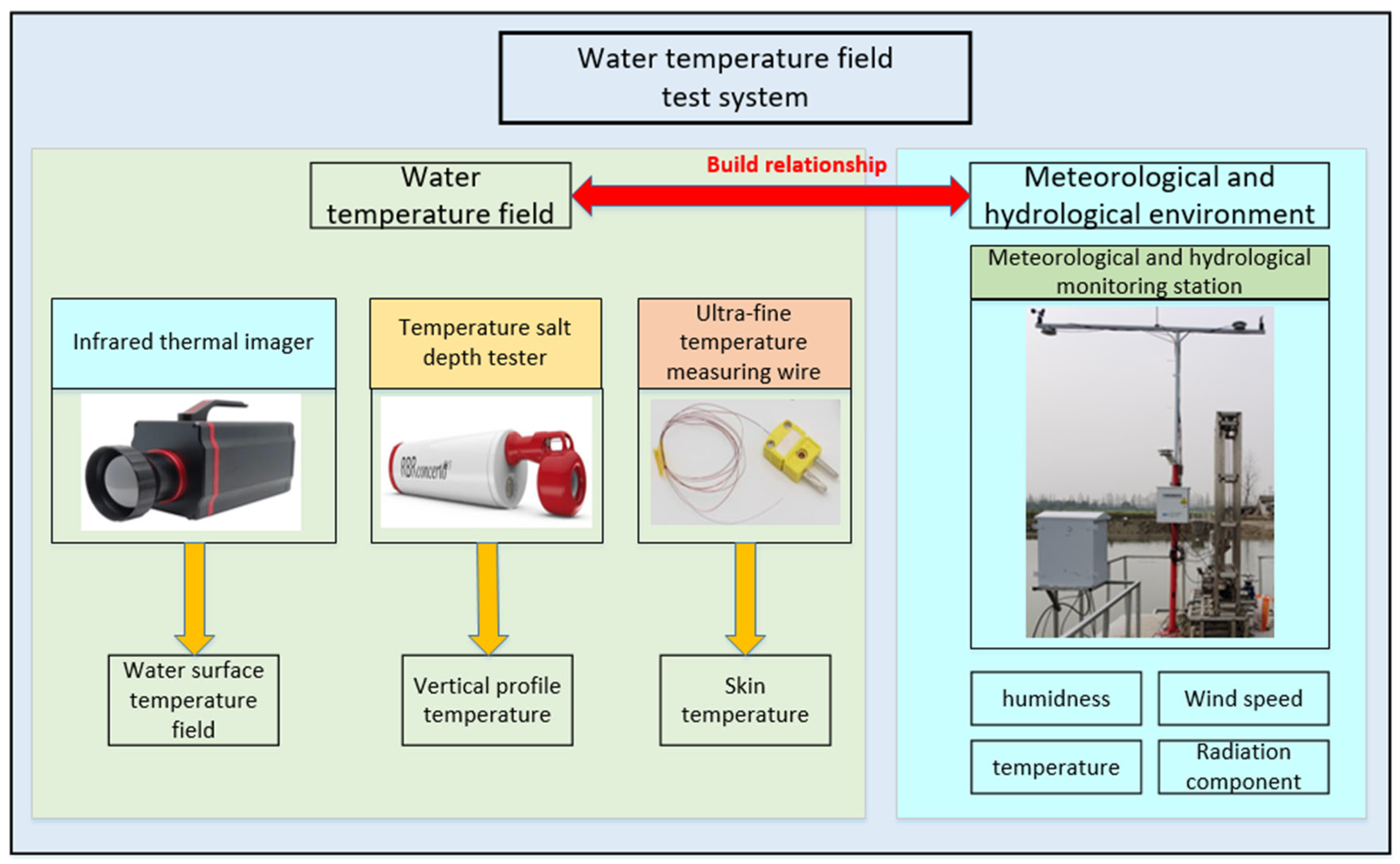
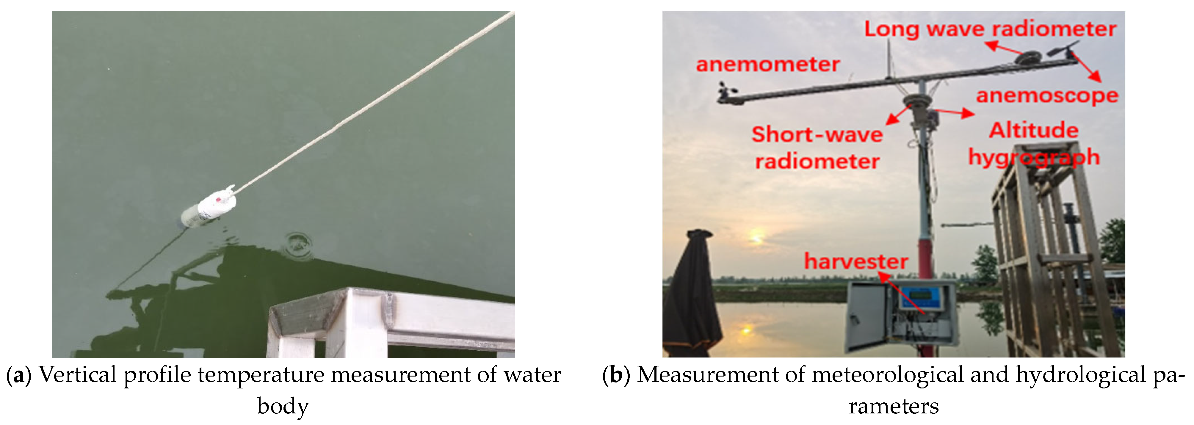
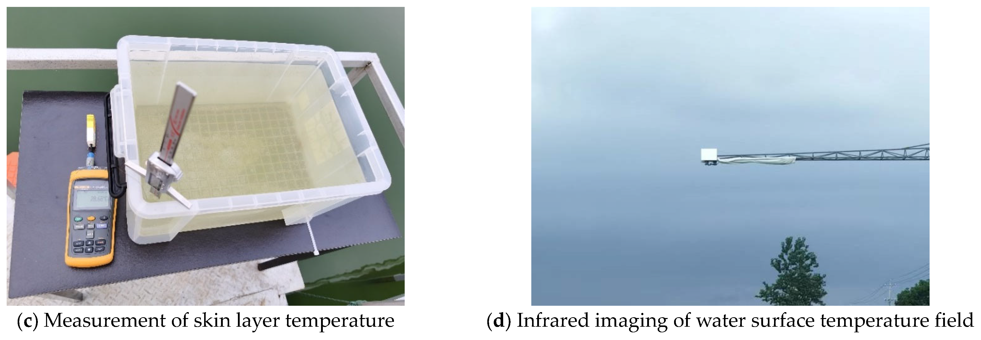
3.1. Experimental Testing System

To establish the relationship between the background temperature field of the water body and the meteorological and hydrological environment, a testing platform for the background temperature field of the water body was developed. This platform employs a Conductivity–Temperature–Depth (CTD) profiler, a mid-wave cooled infrared thermal imager, and ultra-fine thermocouples to measure the vertical profile temperature, surface temperature, and skin layer temperature of the water body, respectively. A multi-parameter integrated meteorological and hydrological station is utilized to simultaneously monitor and record various meteorological and hydrological parameters. By analyzing the evolution of the water temperature field in conjunction with changes in meteorological and hydrological parameters, the influence patterns of these parameters on the water temperature field are elucidated, and the interrelationships between them are established. The composition and interrelationships of the experimental system are depicted in Figure 3.

The customized YG-QXZ multi-parameter integrated meteorological and hydrological monitoring station comprises three main components: meteorological sensors, a meteorological data acquisition unit, and meteorological data acquisition software. It integrates functions for meteorological data collection, storage, transmission, and statistical analysis, enabling the measurement of a wide range of meteorological and hydrological parameters, including atmospheric temperature, humidity, pressure, wind speed, wind direction, solar shortwave radiation, atmospheric longwave radiation, and water body longwave radiation. Specifically, the atmospheric temperature sensor has a measurement range of −40 to 100 °C, a resolution of 0.1 °C, and an accuracy of ±0.1 °C; the atmospheric humidity sensor has a measurement range of 0 to 100%RH, a resolution of 0.1%RH, and an accuracy of ±3%RH; the wind speed sensor has a measurement range of 0 to 70 m/s, a resolution of 0.1 m/s, and an accuracy of ±0.3 m/s; the shortwave radiometer has a measurement range of 0 to 2000 W/m², a spectral range of 300 to 3000 nm, a sensitivity of 7 to 14 µV/Wm⁻², and an accuracy of ±3%; the longwave radiometer has a measurement range of 0 to 2000 W/m² and a spectral range of 3.5 to 50 µm. The IRMC-615MW mid-wave cooled infrared thermal imager is employed to measure the surface temperature field of the water body. This thermal imager utilizes a stirling cooler to maintain a stable operating temperature, with infrared detector elements arranged in a rectangular array within the focal plane. Each pixel in the image corresponds to an independent detection unit that converts infrared radiation into an electrical signal. The thermal imager has a temperature measurement range of 5 °C to 150 °C, a thermal sensitivity of <20 mK, and a resolution of [resolution value]. The RBRconcerto³C.T.D (RBR, Ottawa, ON, Canada) is a submersible Conductivity–Temperature–Depth (CTD) instrument equipped with temperature, pressure, and conductivity sensors, designed for measuring the temperature, depth, and salinity of the vertical profile of the water body. The CTD has a temperature measurement range of −5 °C to 35 °C, a temperature accuracy of ±0.002 °C, a resolution of <0.00005 °C, a depth measurement range of 0 to 200 m, a depth accuracy of ±0.05%FS, and a resolution of <0.001%FS. The K-type ultra-fine thermocouple features a temperature measurement range of 0 to 200 °C, a weld point diameter of <0.3 mm, a wire diameter of 0.2 mm, and a resolution of 0.01 °C.

3.2. Test Content

The experimental campaign was conducted from May to June 2024 at a geographical location of 114°5′44″ East longitude and 30°18′9″ North latitude, with an elevation of 48 m above sea level. The observation target is a freshwater lake. The study period was characterized by consistently clear weather conditions, providing optimal environmental circumstances for the observations. During the experimental process, systematic measurements of atmospheric parameters were performed at a height of 5 m above the water surface, establishing the upper boundary condition for the thermal boundary layer investigation.

We conducted tests on the vertical profile temperature of the water body, wind speed, and solar shortwave radiation to understand the diurnal variations in the vertical profile of the water body. We analyzed the influence of changes in wind speed and solar radiation on the vertical profile temperature of the water body, and compared the results with theoretical calculations to verify the accuracy of the vertical profile temperature calculation model. This part of the testing was primarily concentrated in three distinct time periods during the day and night: 08:00–12:00, 13:00–17:00, and 18:00–22:00. The water profile temperature was measured every 10 min within each time period, as illustrated in Figure 4a. Consequently, 24 data chains were obtained for each time period, resulting in a total of 72 profile data per day. Based on these data, the spatiotemporal distribution of the vertical profile temperature of the water body was reconstructed. During the measurement process, environmental parameters such as wind speed and solar radiation were simultaneously collected, as depicted in Figure 4b, to serve as driving data for analyzing the changes in the vertical profile temperature of the water body.

While measuring the vertical profile temperature of the water body, we conducted measurements of the skin layer properties of the water body during the day and night to understand the variations in the skin layer properties and verify the accuracy of the cold skin calculation model for the water body. Due to the thinness of the water body’s skin layer, typically in the order of millimeters, the CTD thermometer, with a length of 0.44 m and a diameter of 63.25 mm, and its relatively large temperature probe aperture, did not possess the capability to detect the fine temperature profile of the water body’s skin layer. This is because the probe was not fixed at the very top of the instrument, and the instrument body entered the water before the temperature probe during immersion, which to some extent disrupted the temperature distribution of the skin layer. Therefore, considering the thickness range of the skin layer, a K-type ultra-fine temperature measurement wire was employed to test the skin layer temperature. This type of temperature sensor has a weld point diameter of <0.3 mm and a wire diameter of 0.2 mm, meeting the measurement requirements. One end of the probe was fixed to a digital waterproof micrometer, and the other end was connected to a single-channel handheld thermometer. The distance the probe extended into the water was controlled by moving the micrometer, and the temperatures at several discrete points within the skin layer were collected, as shown in Figure 4c. During the testing process, meteorological and hydrological parameters, including wind speed, surface water temperature, high-altitude air temperature, solar shortwave radiation, and downward longwave radiation, were simultaneously collected. Based on the interface heat flux calculation model, the heat flux components at the time of measurement were evaluated, and the intrinsic relationship between heat flux and the skin layer was established. This part of the testing was conducted throughout the day, continuously measuring the cold skin properties of the water body and meteorological and hydrological parameters from 08:00 in the morning to 22:00 at night.

4. Validation of Water Body Temperature Field Calculation Model and Analysis of Test Results

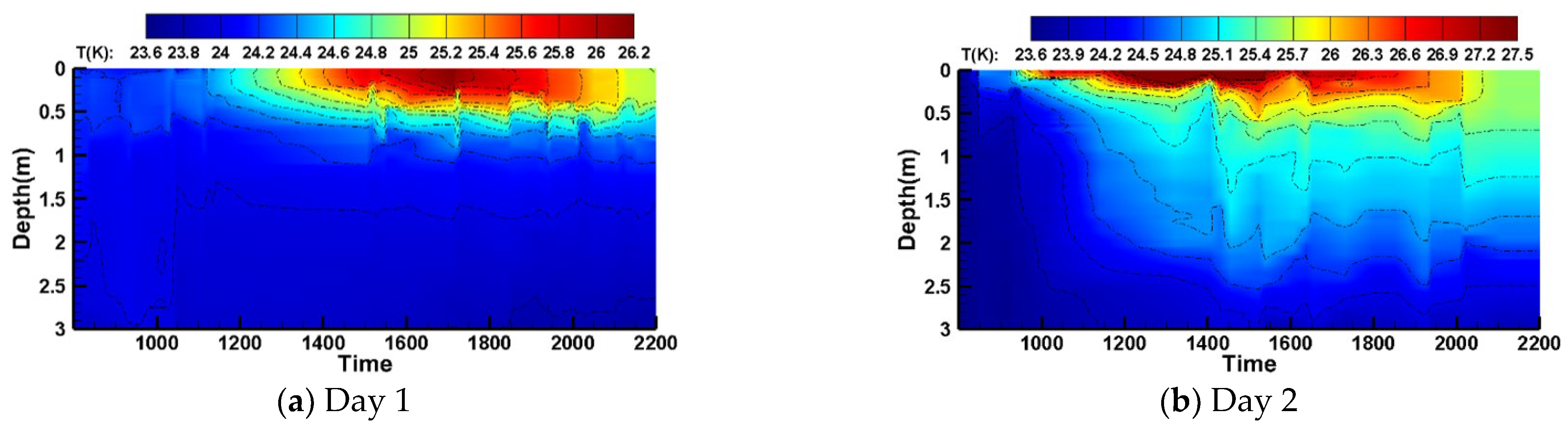
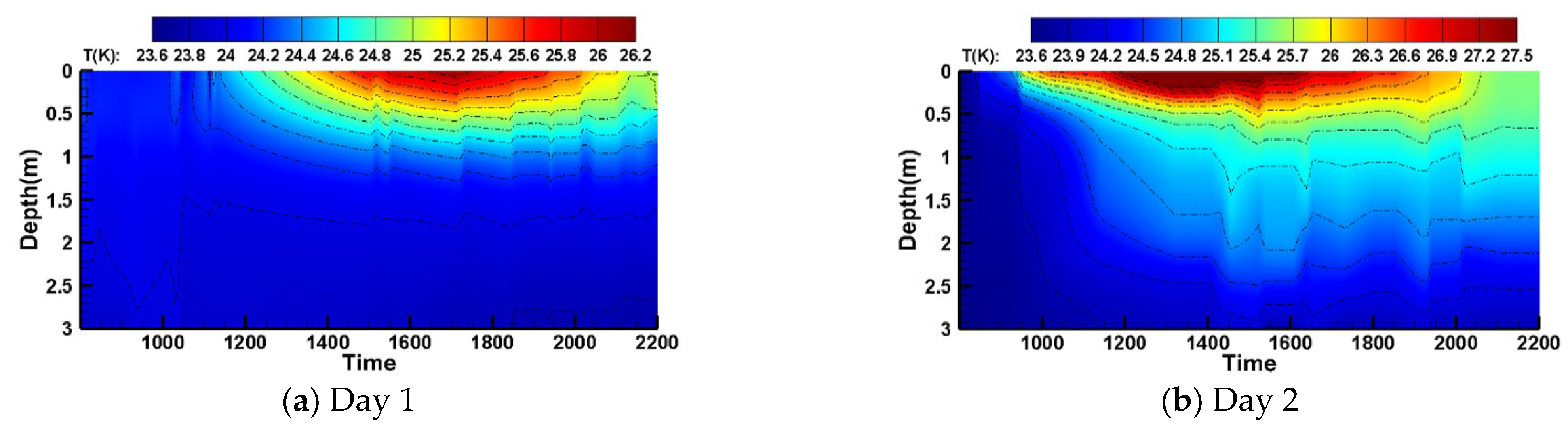
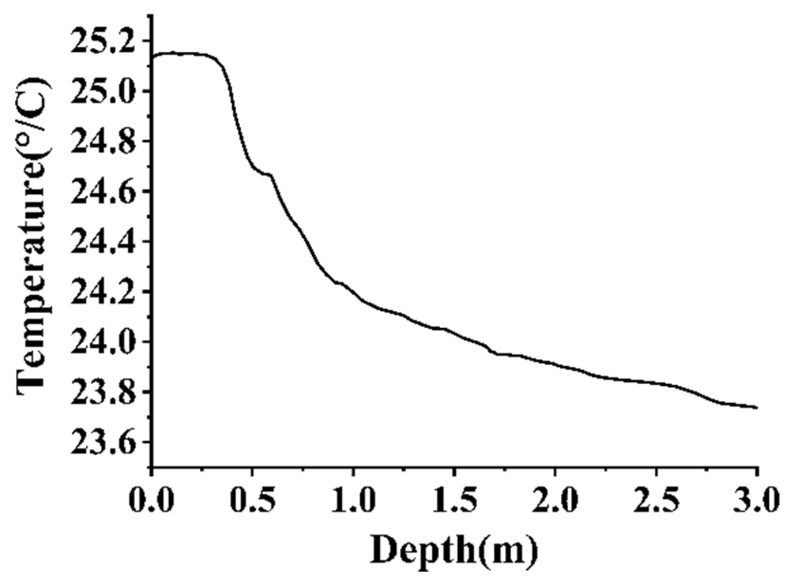
4.1. Spatiotemporal Evolution of Vertical Profile Temperature in Water Bodies

From 08:00 in the morning to 22:00 at night, the vertical profile temperature of the water body was continuously measured using a CTD instrument, resulting in a daily variation color map of the vertical temperature distribution of the water body. Figure 5a,b present the test results for two typical diurnal measurement periods. Figure 6a,b show the corresponding diurnal wind speed and solar shortwave radiation curves over time for the measurement dates. On Day 1, the solar radiation intensity was relatively low, with solar shortwave radiation ranging from 0 to 350 W/m². During the period from 08:00 to 12:00, the solar radiation intensity remained mostly below 200 W/m², while the wind speed stayed at a high level, leading to significant turbulence at the water surface. Consequently, the temperature increase in the upper water layer was relatively slow during this period. From 12:00 to 17:00, the solar radiation intensity gradually increased, and the wind speed decreased, causing the surface water temperature to rise. The heating effect of solar radiation, driven by thermal conduction, gradually diffused downward into deeper water layers, but its influence was limited to within a depth of 1 m. From 17:00 to 22:00, the solar radiation intensity significantly decreased, eventually dropping to zero. During this phase, the water body radiated heat outward, and the surface water temperature gradually decreased. Notably, between 19:00 and 22:00, an isothermal layer formed within the upper 0 to 0.5 m of the water body. During this period, as solar radiation ceased, the water body began to radiate heat outward. The heat exchange between the water body and the atmospheric environment was relatively weak, while a strong temperature gradient existed within the water body. Turbulence between different water layers became dominant, and under the influence of external disturbances and heat conduction, the temperature of the upper water layer redistributed, becoming more uniform. Comparing Figure 6a,b, it is evident that the solar radiation intensity on Day 2 was significantly higher than on Day 1, with a peak exceeding 800 W/m². The range and intensity of the water temperature affected by solar radiation were also notably higher on Day 2. The maximum surface temperature variation on Day 2 reached 3.9 K, and the maximum depth of solar radiation influence extended to 2.3 m. This demonstrates that solar radiation plays a decisive role in the vertical temperature distribution of the water body. Additionally, as shown in Figure 5b, after solar radiation dropped to zero on Day 2, an isothermal layer similar to that on Day 1 formed at the water surface, and the thickness of this layer gradually increased over time.

Figure 7a,b present the diurnal variation simulation results of the vertical temperature profile for Day 1 and Day 2, respectively. Overall, the spatiotemporal evolution of the temperature profile predicted by the computational model aligns well with the measured results. Combined with Figure 8, it can be observed that the discrepancy between the simulated and measured results remains mostly within ±0.2 K across most depths and times. Temporally, the errors are primarily concentrated during periods of high solar radiation intensity, while spatially, they are mainly found in the upper water layers. For Day 1, during periods of high solar radiation, the simulation results show lower temperatures in the upper water layers and higher temperatures in the lower layers compared to the measured data, while the bottom water temperature remains relatively stable. Analysis suggests that the absorption rate of solar radiation in the upper water layers is underestimated in the simulation. In real-world scenarios, the attenuation coefficient of solar radiation in water is strongly influenced by water transparency and quality, determined by factors such as water color and turbidity. However, the computational model assumes an optically uniform water body and does not account for the effects of transparency and water quality. In the lower water layers, the errors primarily stem from the vertical diffusion coefficient. Under varying water depths and wind speeds, the intensity of temperature mixing between layers differs, and the simulation tends to overestimate vertical diffusion in the lower layers. For Day 2, Figure 8b reveals a significant discrepancy between the simulated and measured results around 1400. The measured data show a sharp transition in the temperature profile at this time. According to the solar radiation and wind speed observations, the solar radiation intensity peaked at this moment, while the wind speed remained around 1.5 m/s, showing no significant variation compared to adjacent time periods. Therefore, it is hypothesized that an abnormal fluid vortex disturbance, such as transient turbulence caused by biological activity, may have occurred at a depth of 0.2 m in the measured scenario, interfering with the vertical temperature profile measurement at that time.

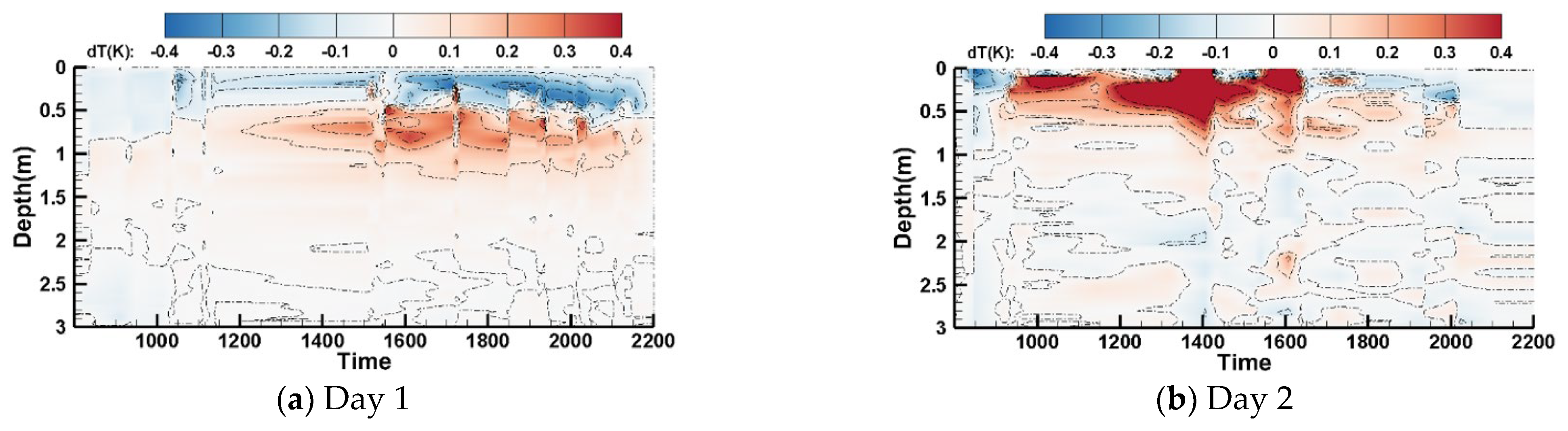
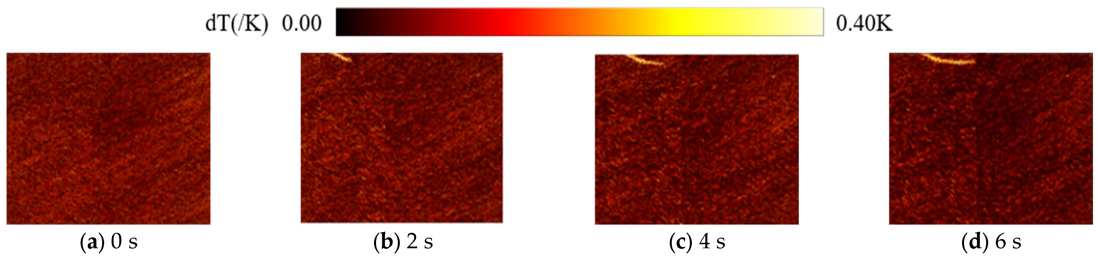
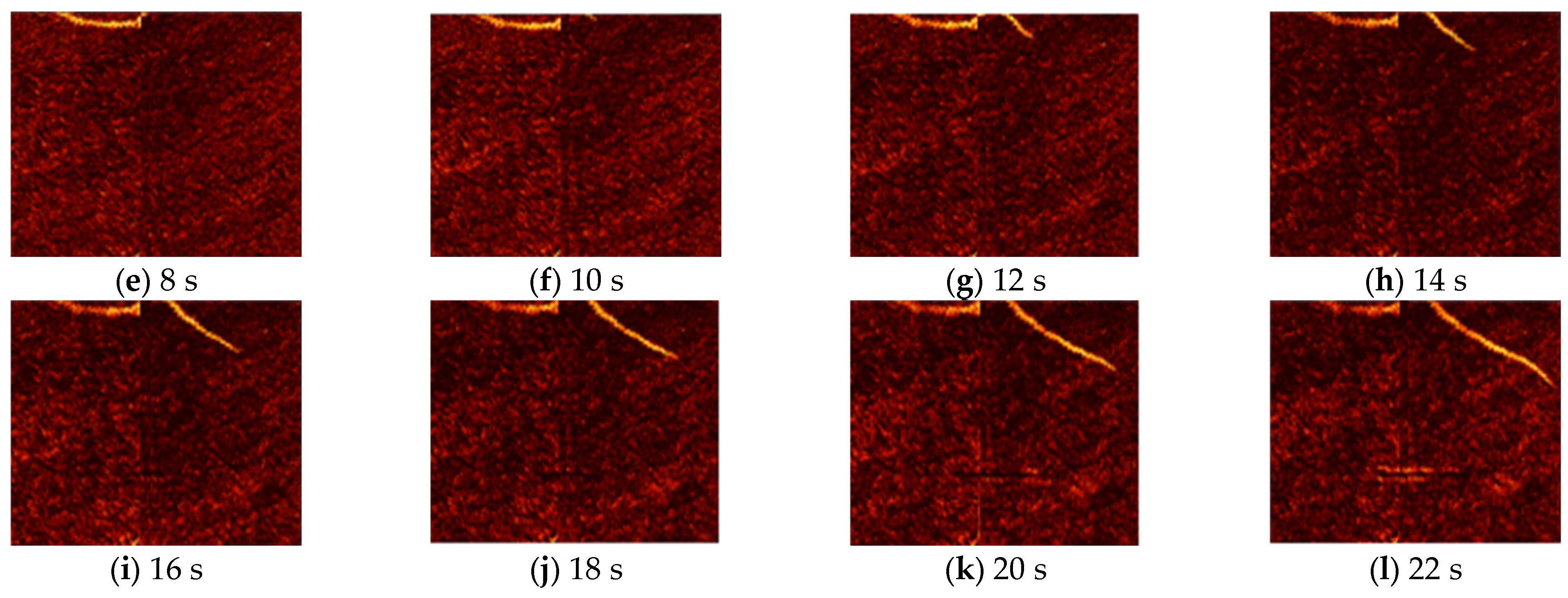
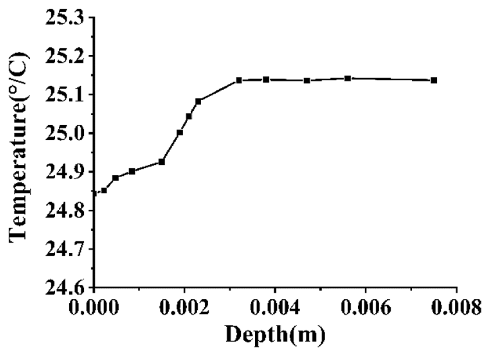
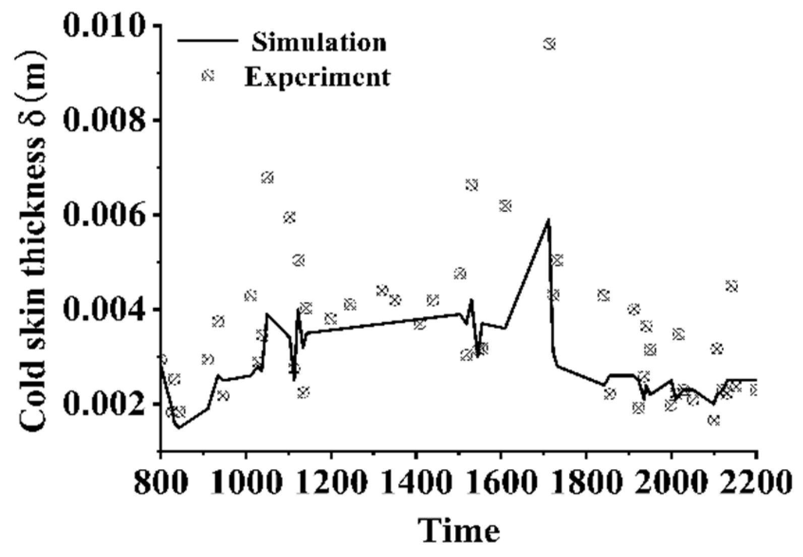
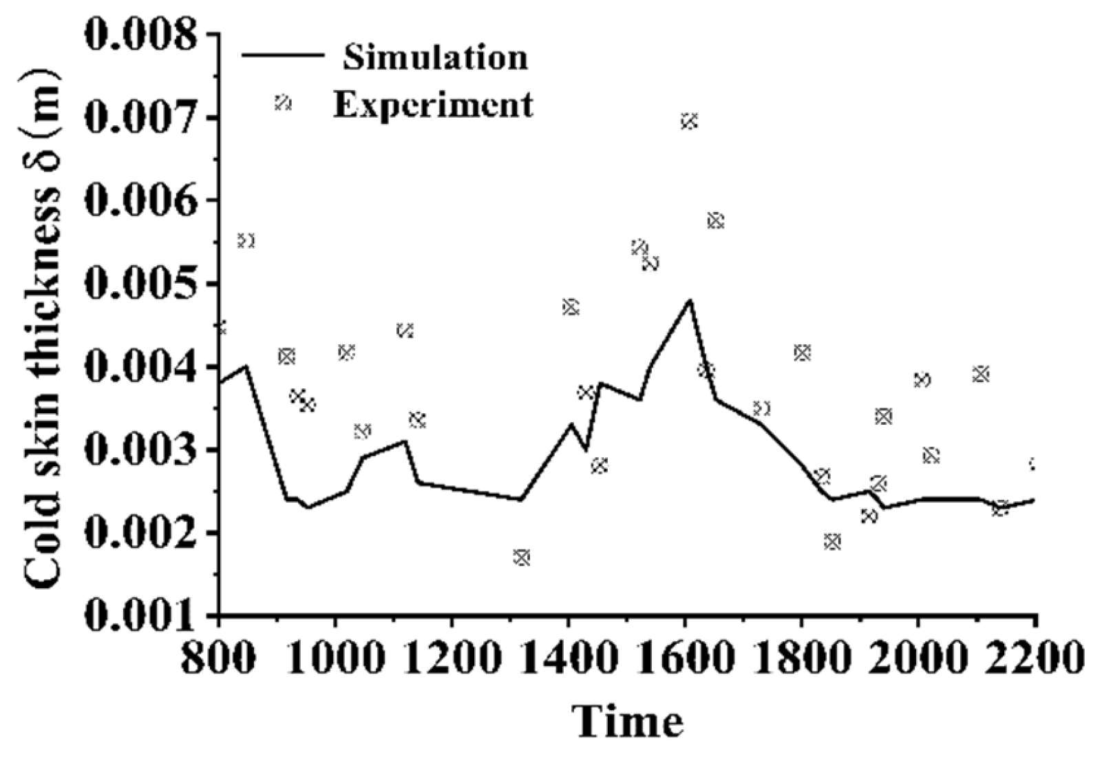
4.2. Verification of the Existence of Cool Skin Layer in Natural Water Bodies

During a particular experiment, an intriguing phenomenon was observed, providing strong evidence for the identification and analysis of the cold skin phenomenon. The experiment was conducted in a natural environment where aquatic organisms were present in the water. During a nighttime test, a small aquatic organism, such as a water coral, swam across the water surface and passed through the infrared field of view, as illustrated in Figure 9. The organism entered the field from the upper left corner, swam downward, made contact with a central wire rope, by-passed it outside the field of view, and then swam diagonally downward to the right of the wire rope before exiting the field. As the organism moved across the water surface, it left behind a distinct “thermal trace”, which was clearly captured by the infrared camera. The length of this thermal trace significantly exceeded the organism’s own size, ruling out the possibility that it was caused by the organism’s thermal radiation. Additionally, the organism’s small size and limited propulsion capability, which relied solely on its own movement, meant it lacked the strong stirring capacity of a ship’s propeller. Consequently, it could not entrain lower water layers to the surface. To further investigate the cause of this phenomenon, the temperature profile of the water body at that moment was measured.

Figure 10 displays the vertical temperature distribution of the water body, as measured by the CTD instrument under the prevailing environmental conditions. The data reveal an isothermal layer within the 0~0.35 m depth range, with a temperature of 25.15 K. Below 0.35 m, the water temperature decreased with increasing depth. Even if the organism had possessed sufficient stirring capability to bring lower water layers to the surface, the surface would have exhibited a “cold” characteristic, making the formation of the “thermal trace” even more perplexing. In the current water environment, the organism was moving within the isothermal layer, while the cold water layer lay beneath it. This raises the following question: why did a thermal trace with a temperature difference of approximately 0.3 K form? Drawing on marine environmental science, it is hypothesized that a temperature boundary layer likely exists at the water surface. The movement of the organism disrupted this boundary layer, resulting in the thermal trace. Extensive literature research in marine hydrometeorology supports this hypothesis [6,9,29,30,42], indicating that in natural environments, factors such as latent heat flux, sensible heat flux, long- and shortwave radiation, wind speed, and air pressure influence the formation of a cold skin at the gas–liquid interface when the net heat flux is positive. This cold skin is typically a few tenths of a degree cooler than the underlying water and is extremely thin, in the order of millimeters. This theoretical framework explains the thermal trace phenomenon: the small organism’s movement disrupted the cold skin’s microstructure at the water–air interface, altering its temperature distribution. To further validate this inference, the temperature distribution of the water surface layer was measured using a single-point method, as shown in Figure 11. The results indicate a low-temperature gradient layer within the 0~2.3 mm range, with temperatures approximately 0.3 K lower than the underlying water layer. This temperature difference aligns closely with that of the thermal trace captured by the infrared thermal imager.

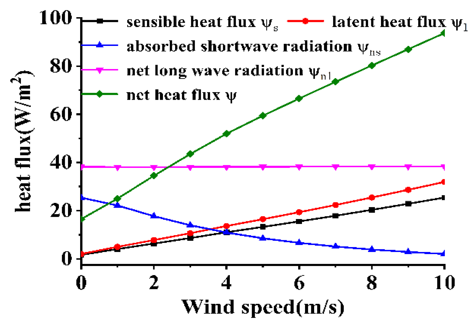
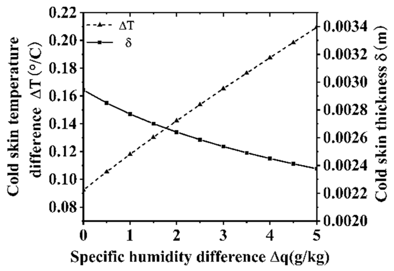
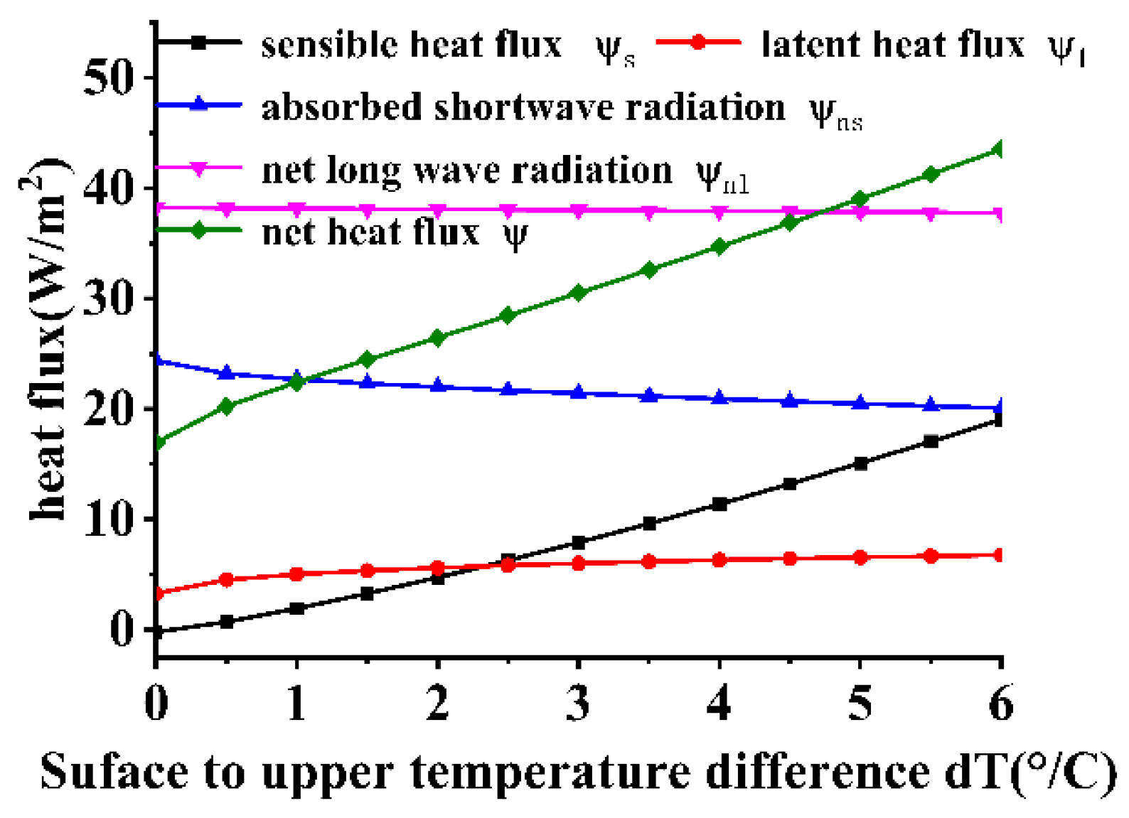
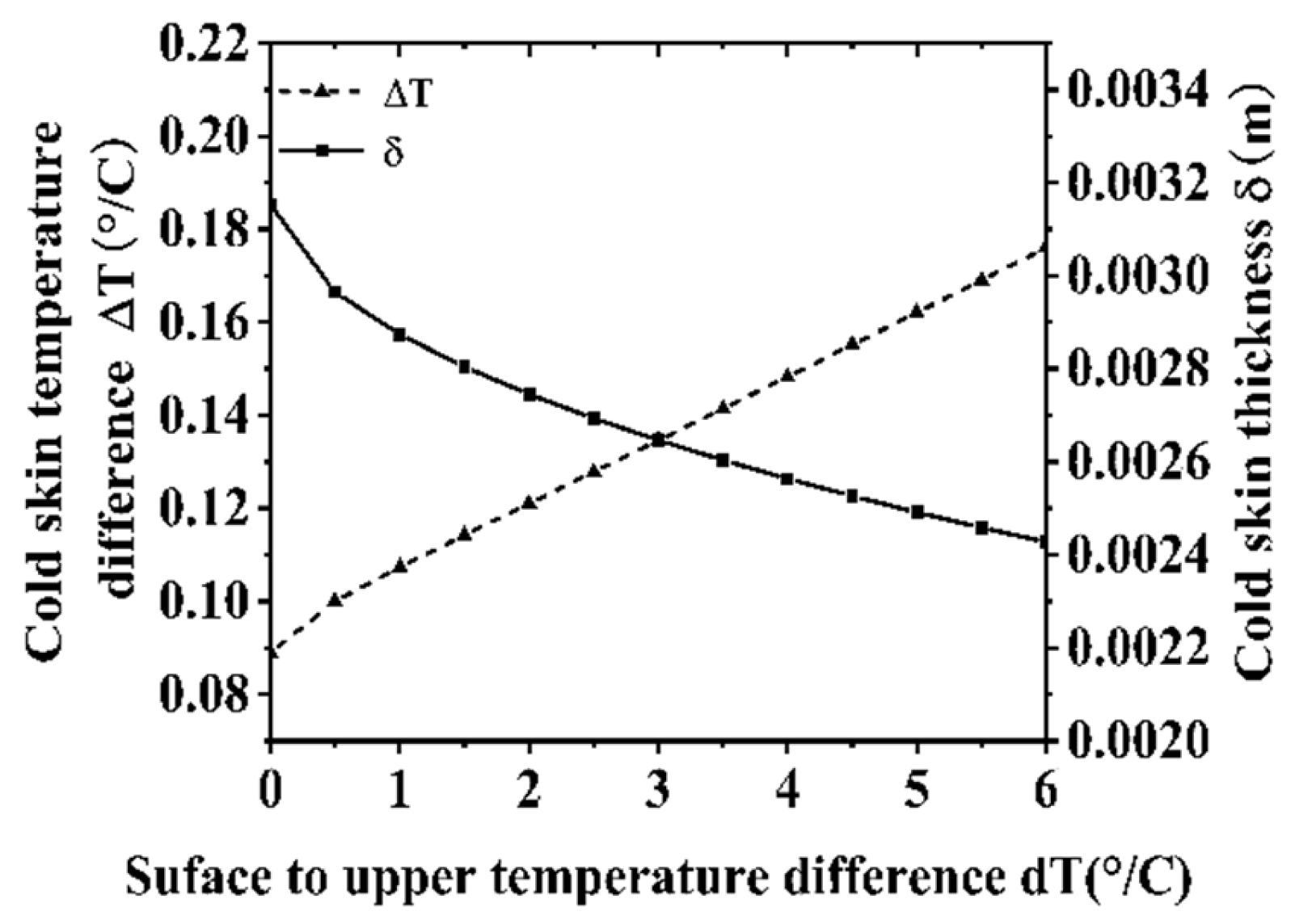
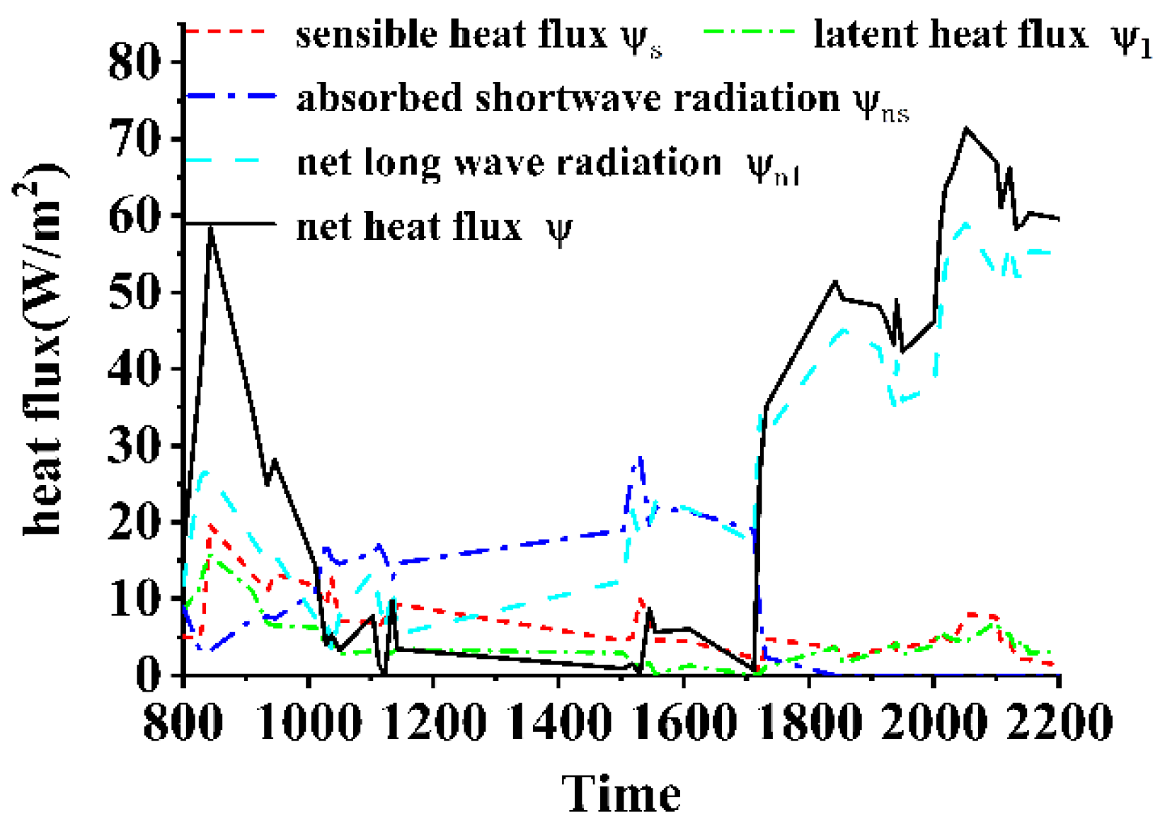
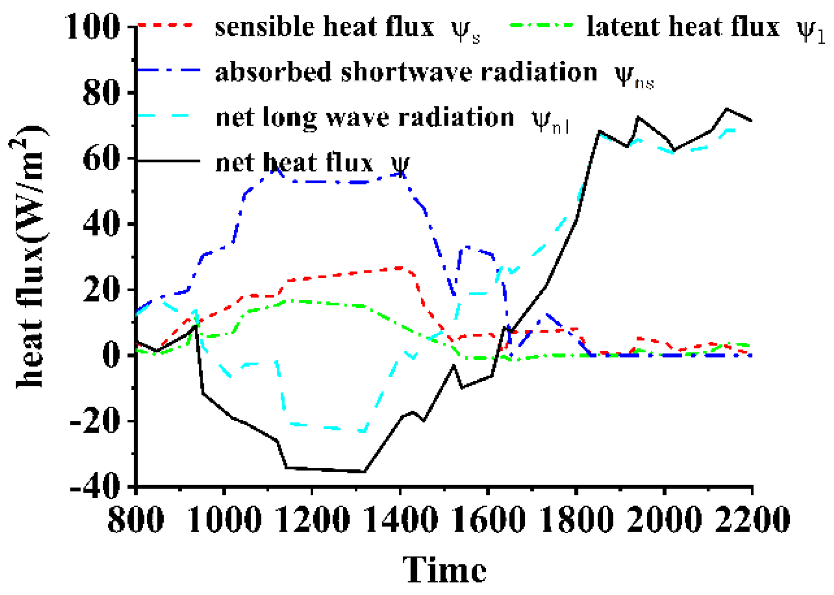
4.3. Analysis of Influencing Factors on the Cold Skin Characteristics of Water Bodies

In Section 4.2, attention was drawn to the cold skin layer on the water surface based on experimental observations, and the underlying formation mechanism of this phenomenon was theoretically identified. The existence of the cold skin was further corroborated through direct measurements of the vertical profile and surface temperature distribution of the water body. To investigate how variations in environmental parameters influence the properties of the cold skin, the cold skin calculation model for water bodies was employed to analyze the effects of changes in parameters such as wind speed, the specific humidity difference between the near-surface and upper-air layers, and the temperature difference between the near-surface and upper-air layers on various heat fluxes and cold skin characteristics.

Figure 12 and Figure 13 depict the variations in heat fluxes at the gas–liquid interface and the properties of the cold skin under varying upper-air wind speeds. In the wind speed range of 0~10 m/s, as the wind speed increases, both the evaporation rate at the water surface and the convective heat exchange between the lower air layer and the surface water body intensify. As a result, the sensible heat flux and latent heat flux exhibit a linear increase with wind speed. Additionally, as wind speed rises, the MOS velocity scale parameter, which governs the thickness of the cold skin, also increases. Since the cold skin thickness is inversely proportional to the velocity scale parameter, the thickness of the cold skin gradually diminishes with increasing wind speed, leading to a reduction in the absorption of shortwave solar radiation within the thin layer. Under the combined influence of these heat fluxes, the net heat flux at the interface increases. The temperature difference of the cold skin is proportional to the product of the net heat flux and the cold skin thickness. In the wind speed range of 0~10 m/s, there exists a critical point at approximately 2.5 m/s, where the temperature difference of the cold skin reaches its maximum value.

Figure 14 and Figure 15 depict the variations in heat fluxes at the gas–liquid interface and the properties of the cold skin under different near-surface to upper-air specific humidity differences. As shown in Figure 14, the near-surface to upper-air specific humidity difference primarily affects the latent heat flux, while its influence on other heat flux components is relatively limited. A larger specific humidity difference signifies a more intense water vapor exchange process between the near-surface air and the upper-air layers. During the upward diffusion of water vapor, the surface water body undergoes continuous evaporation, establishing a sustained water vapor circulation process. This process effectively removes heat from the surface water, contributing to a pronounced cooling effect. The thickness of the cold skin decreases as the specific humidity difference increases, primarily due to the density difference in the medium induced by the specific humidity difference. However, compared to the growth rate of the net heat flux, the rate of decrease in cold skin thickness with increasing specific humidity difference is relatively modest. As a result, under conditions where the net heat flux experiences a significant increase, the temperature difference of the cold skin becomes more sensitive to variations in heat flux, demonstrating a trend of increasing with the specific humidity difference.

Figure 16 and Figure 17 illustrate the variations in heat fluxes at the gas–liquid interface and the properties of the cold skin under different near-surface to upper-air temperature differences. As shown in Figure 16, the near-surface to upper-air temperature difference primarily influences the sensible heat flux, while other heat flux components exhibit minimal sensitivity to changes in this parameter. The physical essence of the sensible heat flux lies in the temperature difference between the lower air layer and the water body, where heat is exchanged through conductive contact between the atmosphere and the water. Therefore, a larger near-surface to upper-air temperature difference indicates a more intense heat exchange process between the media. Typically, during the day when solar radiation is strong, the water body absorbs solar radiation and its temperature rises rapidly. At night, as the air temperature drops, a significant temperature difference develops between the water and the air, resulting in a relatively larger sensible heat flux and a stronger “cooling effect” at the water surface interface. Figure 17 presents the variations in cold skin properties with respect to the near-surface to upper-air temperature difference. The temperature difference of the cold skin increases linearly with the near-surface to upper-air temperature difference, while the thickness of the cold skin decreases as the temperature difference increases. However, the rate of decrease in thickness is slower than the rate of increase in the net heat flux.

4.4. Analysis of the Diurnal Variation Patterns of the Cold Skin Layer in Water Bodies

In Section 4.3, an analysis of the factors influencing cold skin properties provided preliminary insights into how variations in individual environmental parameters affect these attributes. However, in real-world scenarios, these factors interact in a coupled manner. Therefore, this section utilizes environmental parameters measured during Day 1 and Day 2, along with the air–sea flux model and the cold skin calculation model, to compute the diurnal variations in heat fluxes and cold skin properties. These results are then compared with measured data to validate the accuracy of the cold skin calculation model.

Figure 18 illustrates the diurnal variations in heat fluxes for Day 1. It is evident that the sensible and latent heat fluxes remain relatively low throughout the day. During periods of strong solar radiation in the daytime, the water surface absorbs a significant amount of shortwave radiation, which substantially reduces the net heat flux at the interface. At night, when solar radiation ceases, the shortwave radiation absorbed by the water surface drops sharply to zero. At this time, the water temperature exceeds the ambient air temperature, and net longwave radiation dominates, causing the net heat flux at the interface to increase rapidly. This results in an enhanced cooling effect at the water surface during nighttime. Figure 19 presents the calculated and measured results for cold skin thickness. The cold skin thickness predominantly remains within the range of 2–5 mm throughout the day, with minimal diurnal variation. The measured cold skin thickness is generally higher than the calculated values, but the magnitudes are comparable, indicating that the calculation model can predict the cold skin thickness parameter with reasonable accuracy. Figure 20 provides the calculated and measured results for the cold skin temperature difference. Analysis reveals that during the period from 08:00 to 09:40, the sensible and latent heat fluxes remain at relatively high levels, while the shortwave radiation absorbed at the interface is low. This results in a larger net heat flux at the interface, with the cold skin temperature difference ranging between 0.08 and 0.12 K. From 10:00 to 15:30, solar radiation increases significantly, leading to a rise in the radiation absorbed by the water surface and a rapid decrease in the net heat flux at the interface. During this period, the cold skin temperature difference remains at a low level, mostly below 0.02 K. After sunset, the shortwave radiation absorbed at the interface drops sharply, while the net longwave radiation increases steeply, causing the cold skin temperature difference to rise rapidly, exceeding 0.2 K. Figure 20 compares the calculated and measured diurnal variations in the cold skin temperature difference, showing that the trends of the measured and calculated results are generally consistent, with an average error within 23%.

Figure 21 illustrates the diurnal variations in heat fluxes for Day 2. Compared to Day 1, the solar radiation intensity on Day 2 is significantly higher, with shortwave solar radiation exceeding 500 W/m² between 1000 and 1500 and peaking at 800 W/m². During this period, the shortwave radiation energy absorbed by the water surface dominates. Under intense sunlight, the rate of air temperature increase exceeds that of the water temperature, leading to negative net longwave radiation. Although high solar irradiance can enhance water evaporation and heat conduction at the air–liquid interface, the magnitude of this effect is far outweighed by the shortwave radiation energy absorbed at the surface. As a result, the net heat flux at the interface becomes negative. At night, the behavior of the interface heat flux mirrors that of Day 1, with sensible and latent heat fluxes remaining at relatively low levels, while net longwave radiation increases, causing the net heat flux at the interface to rise sharply. Figure 22 presents the calculated and measured results for the cold skin thickness on Day 2. The range of cold skin thickness is consistent with that of Day 1, predominantly remaining within 2–5 mm throughout the day. The measured results align closely with the calculated values in magnitude. Figure 23 shows the calculated and measured results for the cold skin temperature difference. During the daytime period of high solar radiation, a warm skin phenomenon occurs, but the temperature difference is relatively small, around 0.1 K. At night, after solar radiation diminishes, the cold skin temperature difference increases rapidly and stabilizes at approximately 0.2 K. The trends of the measured and calculated results are in good agreement. Day 1 and Day 2 represent two relatively typical measurement days. Over the course of a six-month field experiment, it was observed that solar irradiance significantly influences the measurement results. The analysis reveals that under conditions of high daytime solar irradiance, the temperature difference of the cold skin remains relatively small, and a warm skin phenomenon may even occur.

5. Conclusions

This study develops a model for the evolution of water temperature fields by integrating a heat flux calculation model at the air–liquid interface, a vertical temperature profile calculation model, and a cold skin calculation model, based on the vertical temperature structure of water bodies. The research investigates the spatiotemporal variations in the vertical temperature profile of water, validates the existence of the cold skin phenomenon in natural environments, and analyzes the influence of individual environmental parameter changes on the properties of the cold skin. By considering the diurnal variations in environmental parameters, the study examines the diurnal patterns of cold skin properties and conducts experimental validation. The main conclusions are as follows:

1. The vertical temperature profile of water is primarily influenced by wind speed and solar radiation. At night, an isothermal layer forms in the upper water column. Increased wind speed enhances water turbulence, accelerating heat exchange between different water layers. After solar radiation diminishes at night, the water body radiates heat outward. The heat exchange between the water and the atmosphere is relatively weak, while a strong temperature gradient exists within the water. Under external disturbances and heat conduction, the temperature of the upper water layer redistributes, becoming more uniform and forming an isothermal layer.

2. The cold skin phenomenon is confirmed to exist in natural environments. It is influenced by a combination of factors, including latent heat flux, sensible heat flux, longwave and shortwave radiation, wind speed, and atmospheric pressure. Under certain conditions, a cold skin forms at the air–liquid interface, with a temperature slightly lower (by a few tenths of a Kelvin) than that of the subsurface water. The cold skin is typically very thin, with a thickness on the order of 2–5.0 mm.

3. The properties of the cold skin are mainly affected by wind speed, the near-surface-to-air specific humidity difference, and the near-surface-to-air temperature difference. As wind speed increases, the cold skin thickness gradually decreases. Due to the combined effects of heat flux and cold skin thickness, there exists a critical wind speed at which the temperature difference of the cold skin reaches its maximum. The cold skin thickness decreases with increasing specific humidity difference (or temperature difference), while the cold skin temperature difference increases with increasing specific humidity difference (or temperature difference). Under conditions of high daytime solar irradiance, the shortwave radiation energy absorbed by the water surface dominates, resulting in a small positive or even negative net heat flux at the interface. Consequently, the cold skin temperature difference is small, or a warm skin phenomenon may occur. In contrast, the cooling effect at the interface becomes significantly stronger at night, leading to a larger temperature difference in the cold skin.

References

1. Kawai, Y.; Wada, A. Diurnal sea surface temperature variation and its impact on the atmosphere and ocean: A review. J. Oceanogr. 2007, 63, 721–744. [Google Scholar] [CrossRef]
2. Kawai, Y.; Kawamura, H. Study on a platform effect in the in situ sea surface temperature observations under weak wind and clear sky conditions using numerical models. J. Atmos. Ocean. Technol. 2000, 17, 185–196. [Google Scholar] [CrossRef]
3. Zhang, S.C.; Yang, Z.; Yang, L. Numerical Simulation of Sea Surface Transient Temperature Field. Adv. Mater. Res. 2012, 482, 497–500. [Google Scholar] [CrossRef]
4. Luo, F.; Shuai, C.; Du, Y.; Gao, C.; Wang, B. Experimental on the thermal characteristics of surface wake generated by submerged vehicle. Ocean. Eng. 2024, 297, 116957. [Google Scholar] [CrossRef]
5. Farrar, J.T.; Zappa, C.J.; Weller, R.A.; Jessup, A.T. Sea surface temperature signatures of oceanic internal waves in low winds. J. Geophys. Res. Ocean. 2007, 112, C06014. [Google Scholar] [CrossRef]
6. Zappa, C.J.; Jessup, A.T. High-resolution airborne infrared measurements of ocean skin temperature. IEEE Geosci. Remote Sens. Lett. 2005, 2, 146–150. [Google Scholar] [CrossRef]
7. Piccolroaz, S.; Zhu, S.; Ladwig, R.; Carrea, L.; Oliver, S.; Piotrowski, A.P.; Ptak, M.; Shinohara, R.; Sojka, M.; Woolway, R.I.; et al. Lake water temperature modeling in an era of climate change: Data sources, models, and future prospects. Rev. Geophys. 2024, 62, e2023RG000816. [Google Scholar] [CrossRef]
8. Piccolroaz, S.; Toffolon, M.; Majone, B. A simple lumped model to convert air temperature into surface water temperature in lakes. Hydrol. Earth Syst. Sci. 2013, 17, 3323–3338. [Google Scholar] [CrossRef]
9. Donlon, C.J.; Minnett, P.J.; Gentemann, C.; Nightingale, T.J.; Barton, I.J.; Ward, B.; Murray, M.J. Toward improved validation of satellite sea surface skin temperature measurements for climate research. J. Clim. 2002, 15, 353–369. [Google Scholar] [CrossRef]
10. Minnett, P.J.; Smith, M.; Ward, B. Measurements of the oceanic thermal skin effect. Deep Sea Res. Part II Top. Stud. Oceanogr. 2011, 58, 861–868. [Google Scholar] [CrossRef]
11. MacCallum, S.N.; Merchant, C.J. Surface water temperature observations of large lakes by optimal estimation. Can. J. Remote Sens. 2012, 38, 25–45. [Google Scholar] [CrossRef]
12. White, S.; Silva, T.; Amoudry, L.O.; Spyrakos, E.; Martin, A.; Medina-Lopez, E. The colours of the ocean: Using multispectral satellite imagery to estimate sea surface temperature and salinity on global coastal areas, the Gulf of Mexico and the UK. Front. Environ. Sci. 2024, 12, 1426547. [Google Scholar] [CrossRef]
13. Kong, X.; Li, Y.; Wang, L.; Liu, H. Lake Surface Temperature Retrieval Study Based on Landsat 8 Satellite Imagery—A Case Study of Poyang Lake. Atmosphere 2024, 15, 428. [Google Scholar] [CrossRef]
14. Fedorets, A.A.; Dombrovsky, L.A.; Smirnov, A.M. The use of infrared self-emission measurements to retrieve surface temperature of levitating water droplets. Infrared Phys. Technol. 2015, 69, 238–243. [Google Scholar] [CrossRef]
15. Guo, M.; Zhuang, Q.; Yao, H.; Golub, M.; Leung, L.R.; Tan, Z. Intercomparison of thermal regime algorithms in 1-D lake models. Water Resour. Res. 2021, 57, e2020WR028776. [Google Scholar] [CrossRef]
16. Fedorets, A.A.; Shcherbakov, D.V.; Levashov, V.Y.; Dombrovsky, L.A. Self-stabilization of droplet clusters levitating over heated salt water. Int. J. Therm. Sci. 2022, 182, 107822. [Google Scholar] [CrossRef]
17. Liu, T.; Lee, Z.; Shang, S.; Xiu, P.; Chai, F.; Jiang, M. Impact of transmission scheme of visible solar radiation on temperature and mixing in the upper water column with inputs for transmission derived from ocean color remote sensing. J. Geophys. Res. Ocean 2020, 125, e2020JC016080. [Google Scholar] [CrossRef]
18. O’Carroll, A.G.; Armstrong, E.M.; Beggs, H.M.; Bouali, M.; Casey, K.S.; Corlett, G.K.; Dash, P.; Donlon, C.J.; Gentemann, C.L.; Høyer, J.L.; et al. Observational needs of sea surface temperature. Front. Mar. Sci. 2019, 6, 420. [Google Scholar] [CrossRef]
19. Rahaghi, A.I.; Lemmin, U.; Sage, D.; Barry, D.A. Achieving high-resolution thermal imagery in low-contrast lake surface waters by aerial remote sensing and image registration. Remote Sens. Environ. 2019, 221, 773–783. [Google Scholar] [CrossRef]
20. Hampton, S.E.; Izmest’eva, L.R.; Moore, M.V.; Katz, S.L.; Dennis, B.; Silow, E.A. Sixty years of environmental change in the world’s largest freshwater lake–Lake Baikal, Siberia. Glob. Change Biol. 2008, 14, 1947–1958. [Google Scholar] [CrossRef]
21. Austin, J.A.; Colman, S.M. Lake Superior summer water temperatures are increasing more rapidly than regional air temperatures: A positive ice-albedo feedback. Geophys. Res. Lett. 2007, 34. [Google Scholar] [CrossRef]
22. Tiberti, R.; Rossana, C.; Massimiliano, C.; Andrea, L.; Dario, M.; Daniele, S.; Michela, R. Automated high frequency monitoring of Lake Maggiore through in situ sensors: System design, field test and data quality control. J. Limnol. 2021, 80, 1–19. [Google Scholar] [CrossRef]
23. Carrea, L.; Crétaux, J.F.; Liu, X.; Wu, Y.; Calmettes, B.; Duguay, C.R.; Merchant, C.J.; Selmes, N.; Simis, S.G.H.; Warren, M.; et al. Satellite-derived multivariate world-wide lake physical variable timeseries for climate studies. Sci. Data 2023, 10, 30. [Google Scholar] [CrossRef]
24. Fu, Y.; Zou, C.Z.; Zhang, P.; Wu, B.; Wu, S.; Liu, S.; Wang, Y. A climate data record of atmospheric moisture and sea surface temperature from satellite observations. Earth Syst. Sci. Data Discuss. 2025, 2025, 1–26. [Google Scholar]
25. Sharma, S.; Gray, D.K.; Read, J.S.; O’Reilly, C.M.; Schneider, P.; Qudrat, A.; Gries, C.; Stefanoff, S.; Hampton, S.E.; Hook, S. A global database of lake surface temperatures collected by in situ and satellite methods from 1985–2009. Sci. Data 2015, 2, 150008. [Google Scholar] [CrossRef]
26. Sima, O.; Tang, B.-H.; He, Z.-W.; Wang, D.; Zhao, J.-L. Retrieval of Plateau Lake Water Surface Temperature from UAV Thermal Infrared Data. Atmosphere 2024, 15, 99. [Google Scholar] [CrossRef]
27. Marmorino, G.O.; Smith, G.B.; Bowles, J.H.; Rhea, W.J. Infrared imagery of breaking internal waves. Cont. Shelf Res. 2008, 28, 485–490. [Google Scholar] [CrossRef]
28. Tu, C.Y.; Tsuang, B.J. Cool-skin simulation by a one-column ocean model. Geophys. Res. Lett. 2005, 32. [Google Scholar] [CrossRef]
29. Donlon, C.J.; Robinson, I.S. Observations of the oceanic thermal skin in the Atlantic Ocean. J. Geophys. Res. Ocean. 1997, 102, 18585–18606. [Google Scholar] [CrossRef]
30. Prats, J.; Reynaud, N.; Rebière, D.; Peroux, T.; Tormos, T.; Danis, P.-A. LakeSST: Lake Skin Surface Temperature in French inland water bodies for 1999–2016 from Landsat archives. Earth Syst. Sci. Data 2018, 10, 727–743. [Google Scholar] [CrossRef]
31. Moser, P.M. Applications of Airborne Passive Infrared Mapping Devices to Military Oceanography; U.S. Naval Air Develoment Center: Warminster Township, PA, USA, 1987. [Google Scholar]
32. Wenstop. Maritime Infrared Linesanning Trials Against Submarines; Norwegian Defence Research Establishment: Lillestrom, Norway, 1977. [Google Scholar]
33. Chen, Q.; Lin, Q.; Xuan, Y.; Han, Y. Investigation on the thermohaline structure of the stratified wake generated by a propagating submarine. Int. J. Heat Mass Transf. 2021, 166, 120808. [Google Scholar] [CrossRef]
34. Voropayev, S.I.; Nath, C.; Fernando, H.J.S. Thermal surface signatures of ship propeller wakes in stratified waters. Phys. Fluids 2012, 24, 116603. [Google Scholar] [CrossRef]
35. Wang, C.A.; Xu, D.; Gao, J.P. Surface temperature characteristics of underwater thermal jet based on thermal skin. Appl. Ocean. Res. 2023, 130, 103411. [Google Scholar] [CrossRef]
36. Fairall, C.W.; Bradley, E.F.; Godfrey, J.S.; Wick, G.A.; Edson, J.B.; Young, G.S. Cool skin and warm layer effects on sea surface temperature. J. Geophys. Res. Ocean 1996, 101, 1295–1308. [Google Scholar] [CrossRef]
37. Fairall, C.W.; Bradley, E.F.; Rogers, D.P.; Edson, J.B.; Young, G.S. Bulk parameterization of air sea fluxes for tropical ocean global atmosphere coupled ocean atmosphere response experiment. J. Geophys. Res. Ocean 1996, 101, 3747–3764. [Google Scholar] [CrossRef]
38. Fairall, C.W.; Bradley, E.F.; Hare, J.E.; Grachev, A.A.; Edson, J.B. Bulk parameterization of air–sea fluxes: Updates and verification for the COARE algorithm. J. Clim. 2003, 16, 571–591. [Google Scholar] [CrossRef]
39. Grachev, A.A.; Fairall, C.W. Dependence of the Monin Obukhov Stability Parameter on the Bulk Richardson Number over the Ocean. J. Appl. Meteorol. 1997, 36, 406–415. [Google Scholar] [CrossRef]
40. Paulson, C.A.; Simpson, J.J. The temperature difference across the cool skin of the ocean. J. Geophys. Res. Ocean 1981, 86, 11044–11054. [Google Scholar] [CrossRef]
41. Zhang, Y.; Zhang, X. Ocean haline skin layer and turbulent surface convections. J. Geophys. Res. Ocean 2012, 117, 1–15. [Google Scholar] [CrossRef]
42. Saunders, P.M. The Temperature at the Ocean Air Interface. J. Atmos. Sci. 1967, 24, 269–273. [Google Scholar] [CrossRef]
Figure 1. Thermal stratification temperature profile of water.
Applsci 15 03140 g001
Figure 2. Schematic diagram of water–air interface and heat exchange in water body.
Applsci 15 03140 g002
Figure 3. Structure and relation of water temperature field test system.
Applsci 15 03140 g003
Figure 4. Test diagram of water temperature field.
Applsci 15 03140 g004aApplsci 15 03140 g004b
Figure 5. Color map of temperature evolution in vertical profile of water body.
Applsci 15 03140 g005
Figure 6. Diurnal wind speed and solar shortwave radiation curve with time.
Applsci 15 03140 g006
Figure 7. Simulation results of temperature profiles in water bodies over time and space.
Applsci 15 03140 g007
Figure 8. Time–space evolution error map of vertical temperature profile in water body.
Applsci 15 03140 g008
Figure 9. An infrared temporal map of the ‘heat trail’ left by moving aquatic organisms.
Applsci 15 03140 g009aApplsci 15 03140 g009b
Figure 10. Temperature distribution in vertical profile of water body.
Applsci 15 03140 g010
Figure 11. Temperature distribution in the skin layer.
Applsci 15 03140 g011
Figure 12. Effect of wind speed on each heat flux.
Applsci 15 03140 g012
Figure 13. Effect of wind speed on cold skin properties.
Applsci 15 03140 g013
Figure 14. Effect of specific humidity difference on each heat flux.
Applsci 15 03140 g014
Figure 15. Effect of specific humidity difference.
Applsci 15 03140 g015
Figure 16. Effect of temperature difference on each heat flux.
Applsci 15 03140 g016
Figure 17. Effect of temperature difference on cold skin properties.
Applsci 15 03140 g017
Figure 18. Diurnal heat flux variation curve of Day 1.
Applsci 15 03140 g018
Figure 19. Cold skin thickness calculation and measured results of Day 1.
Applsci 15 03140 g019
Figure 20. Cold skin temperature difference calculation and measured results of Day 1.
Applsci 15 03140 g020
Figure 21. Diurnal heat flux variation curve of Day 2.
Applsci 15 03140 g021
Figure 22. Cold skin thickness calculation and measured results of Day 2.
Applsci 15 03140 g022
Figure 23. Cold skin temperature difference calculation and measured results of Day 2.
Applsci 15 03140 g023