A Convolutional Neural Network Tool for Early Diagnosis and Precision Surgery in Endometriosis-Associated Ovarian Cancer

Abstract

Background/Objectives: The aim of this study was the early identification of endometriosis-associated ovarian cancer (EAOC) versus non-endometriosis associated ovarian cancer (NEOC) or non-cancerous tissues using pre-surgery contrast-enhanced-Computed Tomography (CE-CT) images in patients undergoing surgery for suspected ovarian cancer (OC). Methods: A prospective trial was designed to enroll patients undergoing surgery for suspected OC. Volumes of interest (VOIs) were semiautomatically segmented on CE-CT images and classified according to the histopathological results. The entire dataset was divided into training (70%), validation (10%), and testing (20%). A Python pipeline was developed using the transfer learning approach, adopting four different convolution neural networks (CNNs). Each architecture (i.e., VGG19, Xception, ResNet50, and DenseNet121) was trained on each of the axial slices of CE-CT images and refined using the validation dataset. The results of each CNN model for each slice within a VOI were combined using three rival machine learning (ML) models, i.e., Random Forest (RF), Gradient Boosting (GB), and K-Nearest Neighbor (KNN), to obtain a final output distinguishing between EAOC and NEOC, and between EAOC/NEOC and non-tumoral tissues. Furthermore, the performance of each hybrid model and the majority voting ensemble of the three competing ML models were evaluated using trained and refined hybrid CNN models combined with Support Vector Machine (SVM) algorithms, with the best-performing model selected as the benchmark. Each model’s performance was assessed based on the area under the receiver operating characteristic (ROC) curve (AUC), F1-score, sensitivity, and specificity. These metrics were then integrated into a Machine Learning Cumulative Performance Score (MLcps) to provide a comprehensive evaluation on the test dataset. Results: An MLcps value of 0.84 identified the VGG19 + majority voting ensemble as the optimal model for distinguishing EAOC from NEOC, achieving an AUC of 0.85 (95% CI: 0.70–0.98). In contrast, the VGG19 + SVM model, with an MLcps value of 0.76, yielded an AUC of 0.79 (95% CI: 0.63–0.93). For differentiating EAOC/NEOC from non-tumoral tissues, the VGG19 + SVM model demonstrated superior performance, with an MLcps value of 0.93 and an AUC of 0.97 (95% CI: 0.92–1.00). Conclusions: Hybrid models based on CE-CT have the potential to differentiate EAOC and NEOC patients as well as between OC (EAOC and NEOC) and non-tumoral ovaries, thus potentially supporting gynecological surgeons in personalized surgical approaches such as more conservative procedures.

1. Introduction

Endometriosis (EMS) is a chronic, invaliding, inflammatory gynecological condition affecting about 10% of women of reproductive age [1]. EMS is characterized by lesions of endometrial-like tissue outside the uterus involving the pelvic peritoneum and ovaries. In addition, distant foci are sometimes observed [2]. Unfortunately, little is known about EMS etiology. Although non-malignant, EMS shares similar features with cancer, such as the development of local and distant foci, resistance to apoptosis, and invasion of other tissues with subsequent damage to the target organs. Moreover, patients with EMS (particularly ovarian EMS) show a high risk (about 3 to 10 times) of developing epithelial ovarian cancer (EOC). Epidemiologic, morphological, and molecular studies showed that EMS lesions can progress to ovarian cancer (OC). In fact, patients with EMS (particularly deep infiltrating EMS and ovarian endometriomas) show an increased risk of up to 19 times higher of developing OC The most frequently associated histotypes are represented by clear cell OC (CCC) and endometrioid subtypes.

In advanced stages, OC is the most lethal female gynecological cancer, with median survival rates varying between approximatively 2–7 years based on surgical and chemotherapy outcomes. Some of the most important factors contributing to its late diagnosis are the lack of effective screening tools, as well as the lack of symptoms. OC rapidly spreads over the entire peritoneal surface (carcinosis), thus involving all abdominal organs.

EOC diagnosis and clinical staging are mainly based on imaging exams (CT, ultrasound, PET-CT, and MRI); however, their sensitivity and specificity are suboptimal. Moreover, qualitative imaging often fails to identify different types of lesions (i.e., cancer, borderline, and EMS) in the same patients.

Of note, the reliability of diagnosis, staging, and prognostic evaluation strongly depends on individual training and clinical experience. The typical chronic inflammatory process of EMS involves many factors, such as hormones, cytokines, glycoproteins, and angiogenic factors, which are related to the pathogenesis of the disease. Some of these factors may be expected to perform as EMS biomarkers, together with a variety of other blood markers that have also been investigated during the past decades. In EAOC studies, based on the biomarker hypothesis, changes in levels of analytes, proteins, miRNAs, genes, or other markers could be related to disease stage and patient prognosis. A consistent and biologically relevant categorization can guide clinical management, particularly the choice of targeted therapies and patients’ stratification in clinical trials.

A promising new branch of cancer research is the use of artificial intelligence (AI) and radiomics to recognize patterns in microscopic images and identify novel biomarkers to improve the current diagnostic accuracy and risk assessment of cancer patients.

Several approaches have been proposed in the literature, mainly using the machine learning (ML) model applied to extract the radiomics feature, convolutional neural network (CNN) directly on clinical images or hybrid models (e.g., combining CNN and ML methods).

The most used ML algorithms are Random Forest (RF) [3], Gradient Boosting (GB) [4], and Support Vector Machine (SVM) [5]. Each algorithm has distinct characteristics and mathematical foundations that determine its suitability for specific tasks. RF is a majority-voting ensemble method where multiple classifiers contribute to the final decision by evaluating the margin between the correct class and the alternatives. GB optimizes learning by minimizing a loss function through gradient descent. It follows an iterative process in which a weak learner, typically a decision tree, is sequentially improved to enhance performance. SVM is a supervised classifier that finds the optimal hyperplane to separate two classes by maximizing the margin between their closest data points, known as support vectors [5]. For non-linearly separable data, SVM employs kernel functions to map inputs into a higher-dimensional space, enabling separation [5]. In particular, the SVM algorithm is the most used one reported in the literature [5,6,7,8], in combination with deep learning approaches, due to its complexity (which allows one to obtain more precise results and makes it suitable to be used on small datasets); on the other hand, it is time-consuming since it requests a lot of computational resources [9].

CNNs are deep networks designed for spatially structured data such as images [10]. They consist of convolutional layers that apply filters to extract hierarchical features, followed by pooling layers to reduce dimensionality and enhance translational invariance. The final layers are typically fully connected for classification [10]. Different CNN architectures are employed for bi-dimensional image classification (i.e., tumoral vs. non-tumoral tissue). Transfer learning is widely used in medical imaging to address the challenges posed by small datasets. The most employed CNN architectures are ResNet and VGG-based models [9], which leverage residual blocks to enhance training stability and improve parameter updates in early layers.

The hybrid approach combines CNN with an ML model and extracts features from clinical images by removing the CNN’s final layers and using the extracted features to train the ML model, bypassing the CNN’s classification stage.

A further strategy to improve model performance relies on ensemble strategies, such as the majority voting approach [11]. This approach enhances robustness while reducing overfitting, leveraging the diversity among different underlying input models [12]. In this way, generalization is improved by mitigating individual model biases and limitations [13].

Both CNN and ML models rely on meticulous data processing, balancing, and validation strategies. Data are typically split into training, validation, and test sets, often following a 70:20:10 [14] ratio, ensuring comprehensive model development, hyperparameter tuning, and unbiased evaluation. Addressing data imbalance is critical, as skewed class distributions can degrade predictive accuracy. Solutions such as oversampling, undersampling, or synthetic data generation (e.g., SMOTE) help restore class balance [15]. In CNNs, data augmentation—applying geometric transformations, random cropping, or noise injection—enhances data diversity and mitigates overfitting. Cross-validation [16], e.g., 5-fold, remains a robust standard for performance estimation, optimizing generalizability. These strategies collectively underpin the reliability of ML and CNN models, which are essential for clinical decision-making applications.

To date, no methods have been proposed to distinguish between women with EAOC, NEOC, or OC and benign tissues using pre-operative contrast-enhanced CT (CE-CT) images [17], which are widely used in clinical practice. Currently, a definitive diagnosis requires post-surgical evaluation by a pathologist, limiting personalized surgical approaches due to the absence of pre-surgical biomarkers for the early detection of EAOC.

This study addressed this gap by developing several hybrid AI approaches to differentiate EAOC from NEOC or tumoral vs. non-tumoral lesions using pre-operative CE-CT images. A key novelty lies in the implementation of advanced data processing and balancing strategies, along with a robust model comparison framework leveraging multiple metrics to enhance reliability and predictive performance. Furthermore, the co-creation approach, involving collaboration between clinicians and AI developers, may enhance the model’s usability in clinical settings.

2. Materials and Methods

2.1. Study Design

Patients were enrolled in the Division of Oncologic Gynecology, IRCCS Azienda Ospedaliero-Universitaria di Bologna, between 1 November 2021 and 31 December 2023.

Inclusion criteria were (i) patients with definitive histological diagnosis of OC; (ii) definitive histological diagnosis of EAOC defined as the presence of concomitant EMS and OC in the same patients with/without the presence of atypical endometriosis/borderline lesions; (iii) patients diagnosed with EMS who underwent surgical resection as part of their treatment; (iv) patients with germline mutation of BRCA who underwent prophylactic surgery; (v) high-quality CT-scan available for analysis; (vi) patients treated with primary debulking surgery at our center; (vii) age > 18 years; (viii) written informed consent.

Exclusion criteria included: (i) patients not deemed suitable for surgery; (ii) history of prior pelvic radiotherapy and/or chemotherapy; (iii) patients undergoing neoadjuvant chemotherapy; (iv) non-epithelial OCs and diagnosis of other tumors; (v) recurrent OC.

Figure 1 illustrates the study design, encompassing imaging, data processing, model development, and performance evaluation using various machine learning algorithms and metrics.

2.2. Images and Segmentation

The imaging acquisition parameters used were as follows: mA range: 80–701; kV range: 100–140; helical technique: helix; slice thickness range: 0.625–3 mm; low-osmolality non-ionic iodinated contrast agent administered IV dose: 90–140 mL. CT examinations were performed on the following machines: Siemens SOMATOM Definition Edge, Siemens SOMATOM Definition AS, GE Discovery CT 750HD, GE Lightspeed VCT, GE Revolution Evo, GE Optima CT 660, Philips ingenuity CT 128, Philips Incisive CT, Philips Brilliance 16-slice, and Fujifilm FCT Speedia.

Volumes of interest (VOIs), i.e., right and left ovaries, were segmented on the venous phase of the CE-CT image by an expert radiologist using a semi-automatic approach. It relies on manual segmentation in one of the representative axial slices (generally including the central slice in the cranio-caudal position) and the autopilot function of the MIM software (v. 7.1.4, MIM Software Inc. Cleveland, OH, USA), which helps to guide the segmentation operation in the other slices based on the previous delineations.

2.3. VOI Classification

Final histopathological results were used to label each VOI as EAOC, NEOC, non-tumoral (i.e., ovary without cancer), with EMS or BRCA mutation.

In this study, we used all available data to distinguish between two endpoints, i.e., EAOC versus NEOC or any type of ovarian cancer (i.e., EAOC or NEOC) versus non-tumoral ovaries (i.e., benign EMS or healthy ovaries from patients with mutated BRCA).

Of note, borderline VOIs were excluded.

2.4. Image Pre-Processing and Python Pipeline

CE-CT images were exported from the MIM software in DICOM format for the VOI delineation and exported to Python (version 3.9.13) for the pre-processing operations necessary to arrange the data in a suitable format for the four pre-trained CNNs available in Python [18]. The database was divided with balanced output for each classification investigated (i.e., EAOC vs. NEOC or OC vs. control) in 70% training, 20% testing, and 10% validation. The training dataset was augmented by rotating each CE-CT scan of 30, 45, 90, 325 degrees with respect to the cranio-caudal (CC) axis and axial slices were obtained in each VOI.

To guarantee the convergence of CNN models, greyscale images were rescaled by dividing each pixel by 255, which was the maximum permitted value in each pixel.

Each delineated VOI available on the augmented CE-CT dataset was resized to a 224 × 224 × 128 or to a 299 × 299 × 128 matrix. Each axial slice with a 224 × 224 matrix was used as input in three pre-trained CNNs (i.e., VGG19 [19], ResNet50 [20], and DenseNet121 [21]), while the axial slice with a 299 × 299 matrix was used as input for the Xception CNN [18]. All CNNs were pre-trained with the same dataset, ImageNet [22].

Each axial slice was associated with a binary classification according to the endpoint investigated.

In our dataset, the EROC vs. NEOC class distribution was as follows: 59 samples for the positive class and 95 samples for the negative class, with a 1:1.6 ratio indicating moderated unbalancing. Furthermore, the EROC + NEOC vs. non-tumoral class distribution was as follows: 154 samples for the positive class and 84 samples for the negative class, with a ratio of 1.8:1, indicating moderated unbalancing.

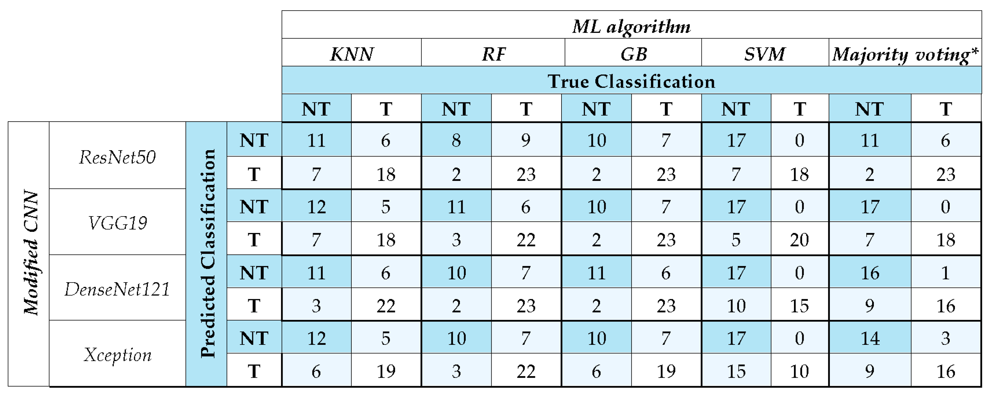
To address the potential class imbalance, we used an undersampling option during the training phase of each CNN algorithm for class balancing. Furthermore, in addition to accuracy, AUC, and F1-score, we evaluated the confusion matrix for the EAOC vs. NEOC class and tumoral (EAOC or NEOC) vs. non-tumoral class to assess the model performance.

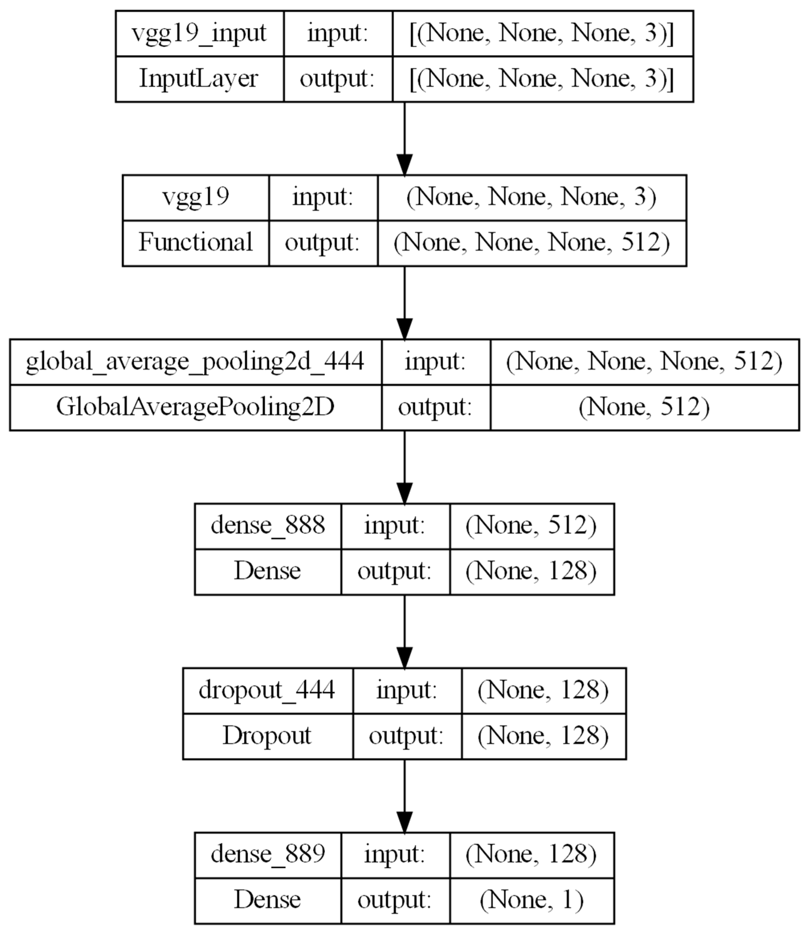
The selected CNNs were trained using a massive dataset to distinguish between 1000 different types of objects [22]. We modified the last four layers to allow for a binary classification while freezing all the other layers to preserve the network’s complexity for image classification. The implemented architecture leverages a pre-trained CNN (e.g., VGG19) as a feature extractor, followed by a GlobalAveragePooling2D layer to reduce spatial dimensions. It includes a Dense layer with 128 neurons, a Dropout layer with L1 penalization to prevent overfitting, and a final Dense layer with one neuron having a sigmoid activation function for binary classification. Each CNN was trained for 100 epochs, with a patience of 50 epochs.

The modified architecture combines transfer learning and task-specific layers for robust image classification; see Figure 2 as an example for the VGG-19 CNN.

Since the CNNs were not able to classify the whole VOI, we customized the CNN architecture to analyze each slice of the VOI. The CNN-predicted results were used as input for the ML algorithms, which were our final meta-classifier to produce a final single classification of the whole VOI.

Finally, three different ML algorithms, available in keras, i.e., K-Nearest Neighbor (KNN), Random Forest (RF), and Gradient Boosting (GB) classifier were used to predict the two classifications. Each ML model was trained using a 5-fold cross-validation, both in fine-tuning and actual training. A grid search approach was used to identify the best combination of hyper-parameters. Since each algorithm has its peculiar kind of hyper-parameters, which can be modified, we had to change the type of hyper-parameters to look for the best set for the ML algorithm: the number of neighbors, weights, and kind of distance for KNN algorithm; the number of estimators, maximum depth and features, and minimum of samples split and leaves for RF; the number of estimators, learning rate, maximum depth and features for GB. The best combination of these hyper-parameters is reported in Table S2 in the Supplementary Material for each ML algorithm.

Overall, we investigated 12 models combining four CNNs as base learners, four ML algorithms as meta-learners, and an ensemble approach (i.e., a voting system based on KNN, RF, and GB). For both learners, a fine-tuning phase to optimize their hyperparameters was run before the actual training and test phases.

Moreover, we compared results obtained with this approach with more solid approaches in the literature for classification tasks, such as the SVM ML algorithm or the majority voting approach [11]. The SVM ML algorithm was developed by following the same approaches previously reported for the other ML models and used as a reference for subsequent comparisons of hybrid approaches.

Finally, an ensemble voting approach was developed by combining the three ML algorithms, i.e., KNN, RF, and GB classifiers. Each model was trained independently on the same dataset, and their predictions were aggregated using a majority voting strategy; the class predicted by most models determined the final classification.

2.5. Performance Metrics

To assess the overall performance of the combined CNN and ML models, we utilized multiple evaluation metrics, including accuracy, the area under the receiver operating characteristic curve (AUC-ROC), and the F1-score. We then compared the results of the CNN and ML algorithms (KNN, RF, and GB) with those obtained using SVM, as well as with a majority voting strategy applied to each of the hybrid algorithms (KNN, RF, and GB). Additionally, we conducted a DeLong test to assess statistically significant differences among the models and analyzed confusion matrices to gain deeper insight into their classification performance, considering the class imbalance in the test dataset.

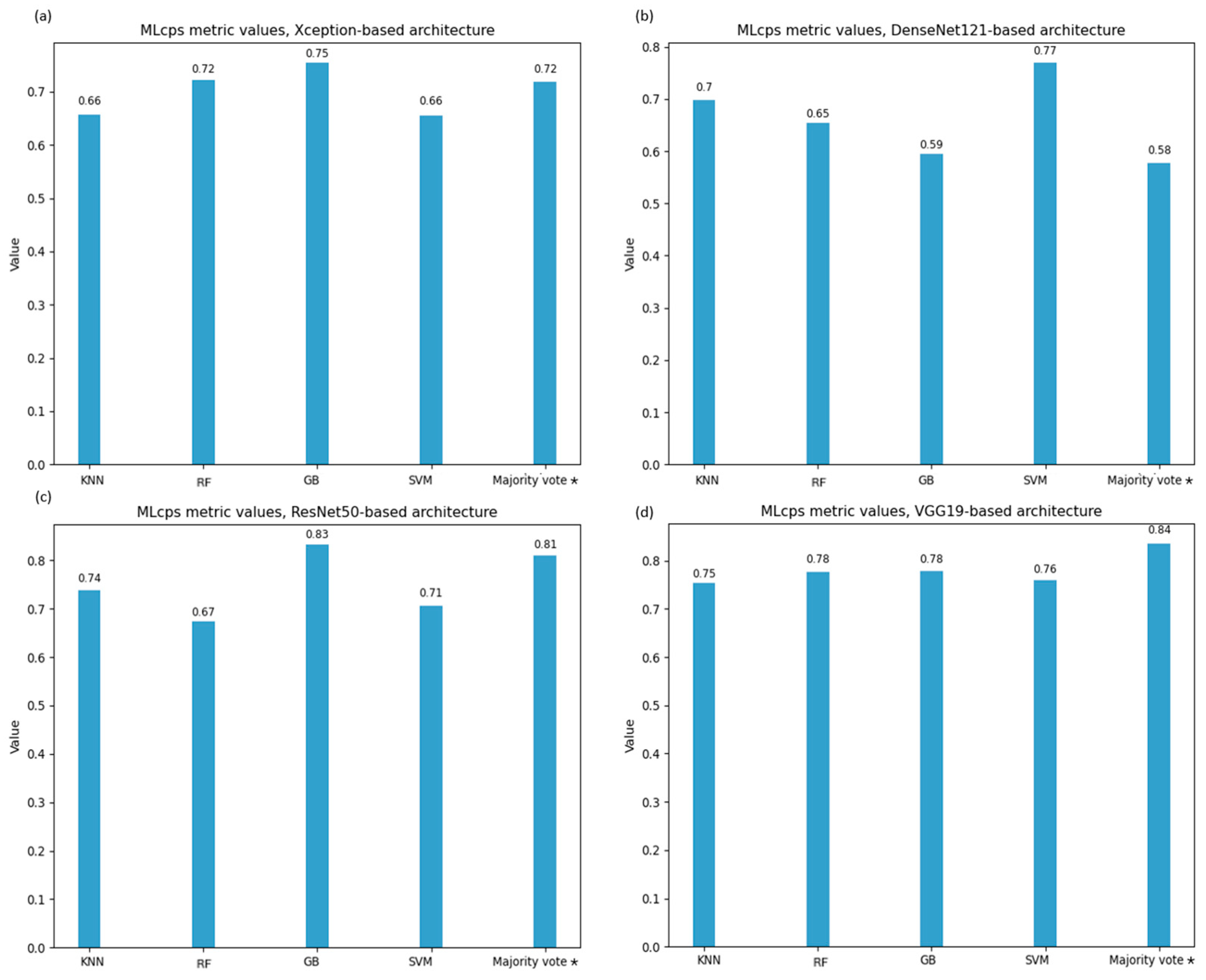
To identify the optimal CNN-ML model combination, we selected the ML cumulative performance score (MLcps) as the evaluation metric [23]. Recognizing the critical importance of accurate prediction using clinical imaging, we adjusted the MLcps weighting scheme to favor models with higher specificity and sensitivity. Specifically, the MLcps was computed using the following normalized weights: 0.1 for AUC-ROC, 0.4 for sensitivity, 0.3 for specificity, and 0.2 for the F1-score.

3. Results

3.1. Enrolled Patients and Characteristics

Out of 264 patients with suspected EOC enrolled in the ATENA trial, 145 were excluded from the presented analysis because they received neoadjuvant chemotherapy before surgery, or because CE-CT images were not available from the PACS, or because histopathological results indicated the presence of metastasis originating from other cancers, or because they presented OC recurrence. Out of the remaining 119, a total of 238 segmented VOIs (i.e., left and right because the pathological results were provided separately for each ovary) were obtained, considering that patients could have only two VOIs. The characterization of these volumes is reported in

Table 1. Table reporting the VOI classification used in this work and according to histopathology.

Classification for Stacking Approach	Histopathological Classification	N° of VOIs
Control (non-tumoral) group	Healthy ovaries (HO)	46
	Ovaries with BRCA mutation	13
	Ovaries with endometriosis	25
Tumoral VOIs	Non-endometriosis associated ovarian cancer (NEOC)	95
	Endometriosis-related ovarian cancer (EAOC)	59
Total delineated VOIs		238

.

3.2. CNN Approaches

Four CNN approaches were developed for each endpoint (e.g., tumoral vs. non-tumoral classification or EAOC vs. NEOC classification).

In the fine-tuning phase, we investigated different values for the dropout rate and L1 penalty, which can be implemented in the structure of the final layers of the CNN architecture. In Table S1 (see Supplementary Materials), we reported the dropout rate and L1 penalty values investigated during fine tuning, reporting in bold the values that resulted in the highest accuracy in distinguishing tumoral vs. non-tumoral. By using a grid search approach, developed in Python pipeline, for each CNN, it was possible to obtain the best combination of dropout rate and L1 penalty, thus achieving the highest accuracy of each architecture.

3.3. Tumoral vs. Non-Tumoral Classification

The hybrid models rely on four CNN base models and four ML meta-learners to distinguish tumoral (EAOC or NEOC) vs. non tumoral tissues (i.e., control group). Table S1 in the Supplementary Materials reports the dropout rates and L1 penalization values used for fine-tuning the final layers of four different deep learning architectures: ResNet50, VGG19, Xception, and DenseNet121. Each architecture was tested with various dropout rates (ranging from 0.0 to 0.8) and L1 penalization values (ranging from 0.0 to 1.0). The values in bold indicate the specific configurations selected for training. The dropout rate helps in preventing overfitting by randomly deactivating neurons during training, while L1 penalization is a regularization technique that encourages sparsity in model weights. This table provides insights into the optimization parameters used in the model’s fine-tuning process, which aims to enhance performance and generalization. The selected values in bold reflect the best-performing configurations for training each architecture.

After training and validating all the models, they were tested on the same test dataset, made up of 42 ovaries (17 non-tumoral and 25 tumoral).

After the 16 models were developed (i.e., CNN coupled with KNN, RF, GB, and SVM), we further implemented four majority voting systems (based on four CNN architectures combined with the KNN, RF, and GB algorithms). Thus, we compared their performances in terms of AUC score and 95% interval confidence (IC), F1-score, sensitivity, and specificity with performances obtained with common and robust approaches in the literature, such as the SVM algorithm and majority voting ensemble.

Table 2. Performance metrics of the 20 hybrid/approaches predicting tumoral versus non-tumoral classifications.

		ML Algorithm
Metric	Modified CNN	KNN	RF	GB	SVM	Majority Voting *
AUC + 95% IC	ResNet50	0.70 [0.56, 0.84]	0.84 [0.72, 0.94]	0.89 [0.79, 0.96]	0.92 [0.84, 0.99]	0.81 [0.69, 0.93]
	VGG19	0.79 [0.66, 0.90]	0.83 [0.70, 0.94]	0.86 [0.75, 0.96]	0.97 [0.92, 1.00]	0.82 [0.70, 0.93]
	DenseNet121	0.78 [0.65, 0.90]	0.86 [0.74, 0.96]	0.87 [0.76, 0.96]	0.89 [0.73, 1.00]	0.78 [0.65, 0.90]
	Xception	0.77 [0.64, 0.89]	0.82 [0.70, 0.92]	0.81 [0.69, 0.92]	0.85 [0.68, 1.00]	0.74 [0.60, 0.88]
F1-score	ResNet50	0.78	0.85	0.88	0.89	0.87
	VGG19	0.82	0.86	0.88	0.97	0.89
	DenseNet121	0.83	0.88	0.87	0.94	0.85
	Xception	0.81	0.85	0.84	0.92	0.81
Sensitivity	ResNet50	0.72	0.92	0.92	1.00	0.92
	VGG19	0.72	0.88	0.92	1.00	1.00
	DenseNet121	0.88	0.92	0.92	1.00	0.92
	Xception	0.76	0.88	0.76	1.00	0.84
Specificity	ResNet50	0.65	0.47	0.59	0.70	0.65
	VGG19	0.71	0.65	0.59	0.80	0.71
	DenseNet121	0.65	0.59	0.65	0.60	0.65
	Xception	0.71	0.59	0.59	0.40	0.65

* Based on KNN, RF, and GB.

reports the values of each metric used to evaluate each model’s performance on the test set. The table compares the performance of different CNN architectures (ResNet50, VGG19, DenseNet121, and Xception) integrated with various ML algorithms (KNN, RF, GB, SVM, and majority voting) across four key metrics: AUC, F1-score, sensitivity, and specificity. Focusing on AUC, SVM achieved the highest AUC across all CNNs, with the best result for VGG19 (0.97), and strong performance for DenseNet121 and Xception (both 0.89). Regarding F1-score, SVM also outperformed other models, with VGG19 achieving the highest F1-score (0.97), followed by DenseNet121 (0.94).

In terms of sensitivity, SVM consistently reached a 1.00 sensitivity across all architectures, making it the best choice for identifying positive cases, while in terms of specificity, VGG19 with SVM had the highest specificity (0.80), ensuring reliable negative classifications. Overall, VGG19 with SVM appears to be the optimal combination, providing the highest AUC, F1-score, sensitivity, and strong specificity. This suggests it is the most balanced model, excelling in both positive and negative classification performance when the task is distinguishing tumoral vs. non tumoral tissues using CECT.

A DeLong test was performed, considering AUC scores and 95% IC reported in Table 2. The results of this test, obtained considering the optimal CNN + SVM algorithm as a reference, are reported in

Table 3. p-value (DeLong test) comparing hybrid models distinguishing tumoral (i.e., EAOC or NEOC) vs. non-tumoral ovary classification versus each CNN + SVM approach, assumed as a reference.

	ML Algorithm
Modified CNN	KNN	RF	GB	SVM	Majority Voting *
ResNet50	0.007	0.24	0.60	-	0.13
VGG19	0.005	0.03	0.06	-	0.02
DenseNet121	0.24	0.74	0.82	-	0.24
Xception	0.44	0.76	0.69	-	0.31

* Based on KNN, RF, and GB. The symbol “-” indicates the reference model for the DeLong test comparison.

.

Figure 3 shows four bar charts illustrating MLcps metric values for different classifiers—KNN, RF, GB, SVM, and Majority Vote—applied to four deep learning architectures: Xception, DenseNet121, ResNet50, and VGG19. In the Xception-based architecture, SVM achieves the highest score of 0.79, followed closely by RF at 0.78, while Majority Vote reaches 0.77. The DenseNet121-based architecture exhibits a strong performance across all classifiers, with SVM obtaining the highest value at 0.86 and Majority Vote at 0.84. ResNet50 demonstrates high classification effectiveness, with SVM leading at 0.88 and Majority Vote following at 0.82. VGG19-based architecture achieves the highest overall results, with SVM reaching 0.93, making it the best-performing classifier, while Majority Vote records 0.87. These results highlight SVM and Majority Vote as the most effective classification strategies across architectures.

Figure 4 shows the confusion matrices for the different ML algorithms combined with different CNN architectures compared with the majority voting ensemble, too. Majority voting generally outperforms individual models, especially in reducing non-tumoral ovary misclassification. SVM shows strong classification performance, particularly for the tumoral ovary class, while GB and RF have variable results depending on the CNN used. These findings reinforce the advantage of ensemble learning in improving robustness and reducing model-specific biases.

3.4. EAOC vs. NEOC Classification

Twelve hybrid models were developed to classify EAOC vs. NEOC tissues. The models were evaluated in a test set comprising 30 ovaries (20 NEOC and 10 EAOC). Table S2 in the Supplementary Materials reports examples of dropout rate and L1 penalization obtained during fine-tuning for identifying EAOC vs. NEOC.

Also in this case, the CNN approaches combined with the three investigated ML algorithms were compared with other ML approaches common in the literature, e.g., SVM algorithm and majority voting strategy.

Table 4. Performance metrics of the 20 hybrid models/approaches predicting EAOC vs. NEOC classification.

		ML Algorithm
Metric	Modified CNN	KNN	RF	GB	SVM	Majority Voting *
AUC + 95% IC	ResNet50	0.84 [0.70, 0.95]	0.76 [0.60, 0.90]	0.88 [0.76, 0.98]	0.76 [0.58, 0.91]	0.83 [0.67, 0.96]
	VGG19	0.86 [0.74, 0.96]	0.86 [0.73, 0.96]	0.86 [0.74, 0.97]	0.79 [0.63, 0.93]	0.85 [0.70, 0.98]
	DenseNet121	0.74 [0.57, 0.89]	0.70 [0.52, 0.85]	0.70 [0.51, 0.85]	0.75 [0.59, 0.88]	0.65 [0.50, 0.80]
	Xception	0.72 [0.54, 0.88]	0.78 [0.61, 0.92]	0.80 [0.65, 0.94]	0.71 [0.55, 0.86]	0.75 [0.58, 0.92]
F1-score	ResNet50	0.72	0.69	0.82	0.80	0.76
	VGG19	0.74	0.75	0.71	0.85	0.80
	DenseNet121	0.62	0.67	0.67	0.82	0.46
	Xception	0.62	0.67	0.70	0.82	0.67
Sensitivity	ResNet50	0.75	0.70	0.85	0.80	0.80
	VGG19	0.85	0.90	0.85	0.90	0.80
	DenseNet121	0.95	0.90	0.75	0.80	0.30
	Xception	0.70	0.90	0.90	0.75	0.60
Specificity	ResNet50	0.70	0.60	0.80	0.50	0.85
	VGG19	0.60	0.60	0.70	0.50	0.90
	DenseNet121	0.40	0.30	0.30	0.70	1.00
	Xception	0.60	0.50	0.60	0.40	0.90

* Based on KNN, RF, and GB.

summarizes the values of each metric used to evaluate the performance of each hybrid model on the test set, classifying EAOC vs. NEOC. The table presents the performance of different CNN architectures (ResNet50, VGG19, DenseNet121, and Xception) combined with various machine learning (ML) algorithms (KNN, RF, GB, SVM, and majority voting) across four evaluation metrics: AUC, F1-score, sensitivity, and specificity. Regarding AUC, VGG19 combined with KNN, RF, and GB achieved the highest AUC (0.86), indicating a strong discriminative ability. Based on F1-score, VGG19 with SVM (0.85) and ResNet50 with GB (0.82) showed the best balance between precision and recall. In terms of sensitivity, DenseNet121 with KNN (0.95) and RF (0.90) demonstrated the highest sensitivity, making it effective in identifying positive cases; while in terms of specificity, the majority voting with DenseNet121 (1.00) exhibited the best specificity, ensuring reliable negative predictions. Overall, VGG19 with SVM appears optimal, offering a strong AUC, F1-score, and sensitivity while maintaining good specificity using as input CE-CT images. Majority voting also achieved high specificity, which may be valuable depending on the classification priority.

Furthermore,

Table 5. Results of DeLong test comparing the CNN + ML algorithm versus each CNN + SVM approach, assumed as a reference, for the EAOC vs. NEOC classification tasks.

	p-Values
CNN	KNN	RF	GB	SVM	Majority Voting *
ResNet50	0.45	1.00	0.24	-	0.53
VGG19	0.46	0.47	0.47	-	0.57
DenseNet121	0.93	0.66	0.66	-	0.35
Xception	0.93	0.53	0.41	-	0.73

* Based on KNN, RF, and GB. The symbol “-” indicates the reference model for the DeLong test comparison.

reports the DeLong test values using the AUC and 95% IC of the SVM algorithm as a reference.

Figure 5 presents the MLcps metric values of the 20 hybrid models grouped based on the CNN architecture. More in detail, Figure 5 illustrates four bar charts comparing MLcps metric values for different classifiers—KNN, RF, GB, SVM, and Majority Vote—across four deep learning architectures: Xception, DenseNet121, ResNet50, and VGG19. In the Xception-based architecture, GB achieves the highest value of 0.75, while KNN and SVM perform similarly at 0.66, and Majority Vote reaches 0.72. In the DenseNet121-based architecture, SVM shows the best performance with 0.77, whereas GB has the lowest value at 0.59, and Majority Vote records 0.58. ResNet50 demonstrates strong results, with GB achieving the highest score of 0.83, followed closely by Majority Vote at 0.81. The VGG19-based architecture shows the best overall performance, with Majority Vote reaching 0.84 and GB and RF performing equally at 0.78. ResNet50 and VGG19 appear to be the most effective architectures, particularly when using GB and Majority Vote classification strategies.

Figure 6 shows the confusion matrices for the different ML algorithms combined with different CNN architectures, compared with the majority voting ensemble, too. Majority voting generally outperforms individual models, especially in reducing non-tumoral ovary misclassification. SVM shows a strong classification performance, particularly for the tumoral ovary class, while GB and RF have variable results depending on the CNN used. These findings reinforce the advantage of ensemble learning in improving robustness and reducing model-specific biases.

4. Discussion

Ovary cancer, particularly when arising from endometriosis, represents a rare but clinically significant entity requiring tailored therapeutic strategies due to differing disease outcomes.

While MRI remains the gold standard for preoperative evaluation, its limited availability—due to long acquisition times and the restricted number of scanners—often necessitates the use of CE-CT as a more accessible alternative. Although CE-CT generally offers a lower image quality compared to MRI, AI-driven analysis can extract clinically relevant information that may not be visible to the human eye. This study demonstrates that despite MRI’s superiority in qualitative assessment, CE-CT can provide significant quantitative data through advanced image processing techniques, enhancing its diagnostic value and broadening its applicability in centers where MRI access is limited. Moreover, to mitigate the variability introduced by scanners from different vendors, our institution implements regular quality assurance programs, including protocol harmonization and optimization conducted by medical physicists, ensuring standardized imaging conditions for a more reliable AI-driven analysis.

This is the first prospective study demonstrating that CE-CT can provide significant quantitative information, moving beyond traditional qualitative assessment. By leveraging advanced image analysis, we enhanced the predictive value of CE-CT, offering crucial insights to support gynecological surgeons in optimizing surgical planning. This novel approach paves the way to a more personalized surgical strategy, with the potential for widespread adoption across numerous centers, ultimately improving patient outcomes in this challenging disease subset.

However, the number of cases of rare diseases such as gynecological cancer is also generally limited in oncological HUB centers such as the IRCCS AOUBo. Given this limitation, our study adopts transfer learning [23] and data augmentation to overcome data scarcity [24,25,26]. These techniques enhance model performance, facilitating early detection and differentiation of ovarian cancers while reducing computational costs [10]. By leveraging pre-trained CNNs and stacking approaches, we improve classification accuracy despite the dataset size constraint.

Traditional CNN architectures extract features from 2D medical images, such as MRI and ultrasound, to develop diagnostic models. Previous studies have applied U-Net-based segmentation to small CT datasets, including one limited to a cohort of 20 patients with ovarian cancer [27]. In contrast, our approach leverages a significantly larger, prospectively collected CE-CT dataset with a pathology-confirmed diagnosis at the level of each ovary. By integrating data augmentation and a hybrid AI strategy, we enhance the differentiation of NEOC from non-cancerous tissues and EAOC from NEOC, addressing key diagnostic challenges.

This study implemented several AI-based approaches using four pre-trained CNNs as base-learners combined with four ML algorithms as meta-learners to distinguish EAOC from EOC and tumoral from non-tumoral ovaries, alongside a voting system based on KNN, RF, and GB. The CNN architectures were selected for their accessibility via the Keras package (Python) and their proven performance in transfer learning for classification tasks. The CNN architecture was modified by freezing layers and substituting the final four to optimize binary classification, with fine-tuning focused on the last layers (L1 penalization and dropout rate). The ML models were chosen for their minimal assumptions, such as KNN’s reliance on local data similarity [28], RF’s robustness to outliers [3], GB’s error reduction through boosting [4], and SVM’s ability to handle small, complex datasets. Multiple performance metrics were used to evaluate the hybrid models, with twenty stacking models fine-tuned for binary classification. The developed hybrid models were ranked in terms of MLcps, and a statistical test (e.g., Delong test) was used to check whether models were equivalent or not.

To our knowledge, this is the first study to classify EAOC versus NEOC and the most extensive study distinguishing EAOC vs. NEOC, assessed using histological analyses, and tumoral versus non-tumoral ovaries using CE-CT images. Another significant innovation in this study is the introduction of the MLcps weighted metric as a key performance metric, which emphasizes sensitivity and specificity. This is the first time such a metric has been used to assess a transfer learning approach in ovarian cancer classification tasks, providing a more targeted way to evaluate performance. The use of this metric helps to prioritize critical factors for medical diagnoses, setting this study apart from previous research that lacked such a tailored evaluation approach. All the investigated endpoints were confirmed by the definitive pathology.

Out of the developed models, the ResNet50 model coupled with Gradient Boosting resulted in the highest F1-score of 0.82 and AUC value [95% CI] of 0.88 [0.76, 0.98] in distinguishing EAOC and NEOC. VGG19 exhibited performance comparable to ResNet50, with both surpassing DenseNet121 and Xception. The error analysis carried out using confusion matrices highlights these differences in classification more prominently. ResNet50 and VGG19 coupled with GB and majority voting achieved the highest correct classifications, reinforcing their robustness. SVM exhibited stable performance across models, particularly excelling with VGG19. Conversely, KNN consistently underperformed, highlighting its limitations in this classification task. Majority voting improved overall accuracy, suggesting the advantage of ensemble strategies in mitigating individual model biases.

This performance difference can likely be attributed to variations in network depth and architectural design. Specifically, VGG19, with 19 layers, relies on a simple sequential architecture of convolutional layers, while ResNet50 features 50 layers and leverages residual connections to combat vanishing gradients and improve feature learning in deeper networks. In contrast, DenseNet121 (121 layers) utilizes dense connectivity to encourage feature reuse, and Xception employs depth-wise separable convolutions for computational efficiency, which might trade off some of the features learning capacity. These design differences impact the networks’ ability to learn and generalize effectively [29]. The performance of CNN coupled with SVM reached a similar one to the other ML approaches for distinguishing EAOC vs. NEOC except for Xception + SVM. The voting system based on KNN, RF, and GB achieved a similar performance.

A similar behavior was observed for tumoral vs. non-tumoral classification. Out of the twenty models, the AUC ranged from 0.70 [0.56, 0.84] (ResNet50 + KNN) to 0.97 [0.92, 1.00] (VGG19 + SVM), while F1-score ranged from 0.78 (ResNet50 + KNN) to 0.88 (VGG19 + SVM), sensitivity from 0.72 (ResNet50 + KNN) to 0.92 (VGG19 + SVM), and specificity from 0.59 (DenseNet121 + RF) to 0.80 (VGG19 + SVM). In this endpoint, CNN combined with SVM performed excellently in distinguishing tumoral from non-tumoral ovaries, while the voting system (KNN, RF, GB) showed comparable performance across metrics and MLcps. GB achieved high MLcps scores, confirming its efficiency, while RF performed similarly to previous studies [30,31]. As expected, KNN showed the lowest performance [32]. GB and RF were further validated by comparison with SVM and majority voting, which outperformed individual models. SVM excelled in handling high-dimensional, imbalanced datasets [5] while majority voting improved accuracy and generalization by reducing model bias [11]. Analysis error through confusion matrices showed that ResNet50 and VGG19 coupled with GB and majority voting achieved the highest correct classifications, confirming their reliability. SVM also performed well, particularly with VGG19, while KNN showed weaker results. Majority voting consistently improved classification accuracy, reinforcing the advantage of ensemble methods in reducing individual model biases and enhancing robustness in medical imaging tasks. Overall, the differences among models are likely due to the adopted architecture affecting the overall performance, for tumoral vs. non-tumoral classification, too.

This discrimination is an endpoint generally investigated using magnetic resonance imaging (MRI) performed with multiple types of sequences [17]. Using this imaging modality, Wang et al. [33] classified with homemade CNN 545 ovarian lesions as benign or malignant, using a dataset confirmed by either pathology or imaging follow-up, reporting an AUC of 0.91 ± 0.05 and an F1-score of 0.87 ± 0.06. A similar approach was implemented by Saida et al. [34] to distinguish malignant and benignant ovaries, defined based on the consensus of the two radiologists, with AUC values ranging from 0.83 to 0.89, accuracy ranging from 0.81 to 0.87, sensitivity from 0.77 to 0.85, and specificity from 0.77 to 0.92. Moreover, Mingxiang et al. [35] used the T2-weighted MRI to distinguish between type I and type II NEOCs with a cohort of 437 cancer patients with an AUC [95% IC] of 0.86 [0.786, 0.946]. Similar results on CT images were reported by Kodipalli A. et al. [27] on 20 patients (i.e., 2560 benign and 2370 malignant slices) with the U-Net approach (based on VGG16 and ResNet152 combined with RF and Gradient Boosting) to segment and classify lesions in the ovarian district with the F1-score ranging from 0.819 to 0.918. Of note, we used a larger dataset of 119 CE-CT images (i.e., 10,752 benign and 19,712 malignant slices) analyzed with both ResNet50 and VGG19 associated with a GB algorithm, resulting in an F1-score of 0.880. These results seem promising considering that CE-CT is expected to have a lower image quality when compared to multiple sequences of MRI when used for diagnostic purposes by expert radiologists, thus suggesting that AI-based approaches can reveal details not visible by human eyes.

Moreover, the accessibility of MRI is often limited by long acquisition times and the limited number of scanners relative to CT modality. For this reason, several attempts to use alternative imaging, including ultrasound (US), have been explored. Martinez-Mas et al. [36] used a pure ML approach on a dataset comprising 187 ovarian US images (112 benign, 75 malignant), obtaining an AUC of 0.877 with an SVM algorithm.

Regarding data quality, while CE-CT generally offers a lower image quality than MRI, AI-driven CT analysis presents a compelling alternative due to the widespread availability and rapid acquisition of CT scans. This advantage makes CT-based AI models particularly valuable in clinical settings where MRI access is restricted, broadening their potential impact on ovarian cancer diagnostics. Our dataset was generated in a prospective study founded by the Italian Ministry of Health (ENDO-2021-12371926), thus guaranteeing the possibility to use harmonized protocols for CE-CT acquisition. On the contrary, most of the above-mentioned studies refer to retrospective datasets.

Regarding automatic segmentation, significant efforts have been made to extend its application from ultrasound (US) imaging to various types of medical images [37,38]. Different segmentation techniques have been implemented for CT acquisitions; they are mainly divided into methods based on texture features and methods based on gray-level features, including amplitude segmentation based on histogram features, edge-based ones, and region-based ones [39]. In this context, AI-based algorithms can be seen as tools to further optimize these basic techniques. Nevertheless, although several AI-based tools for the automatic segmentation of organs have been developed and proven to reduce variability among young and experienced physicians [40], to the best of our knowledge, no software for automatic ovary segmentation is currently available for CT images. This is because the ovarian tissue has similar Hounsfield Unit (HU) values to those surrounding tissues. Moreover, ovaries are challenging to detect even for radiologists without experience in the gynecological field. For this reason, obtaining a large database of contoured ovaries—essential for the training, testing, and validation of robust AI-based models—is particularly difficult. Thus, the possibility of using fully automatic segmentation can be considered a possible further improvement of our predictive models.

A further limitation of our approach is the lack of standardized guidelines for selecting weights in MLcps generation. While all metrics showed similar behavior, no single metric alone could define the optimal model, highlighting the challenge of performance evaluation across test datasets.

5. Conclusions

DL-based models using CE-CT images have great potential in differentiating EAOC versus NEOC or malignant tumors versus controls, thus representing valuable and objective information to support the clinical decision in the implementation of fertility-sparing approaches.

References

1. Koninckx, P.R.; Fernandes, R.; Ussia, A.; Schindler, L.; Wattiez, A.; Al-Suwaidi, S.; Amro, B.; Al-Maamari, B.; Hakim, Z.; Tahlak, M. Pathogenesis Based Diagnosis and Treatment of Endometriosis. Front. Endocrinol. 2021, 12, 745548. [Google Scholar] [CrossRef] [PubMed]
2. Amro, B.A.-O.; Ramirez Aristondo, M.E.; Alsuwaidi, S.; Almaamari, B.; Hakim, Z.; Tahlak, M.; Wattiez, A.; Koninckx, P.A.-O. New Understanding of Diagnosis, Treatment and Prevention of Endometriosis. Int. J. Environ. Res. Public Health 2022, 19, 6725. [Google Scholar] [CrossRef] [PubMed]
3. Breiman, L. Random Forests. Mach. Learn. 2001, 45, 5–32. [Google Scholar] [CrossRef]
4. Friedman, J.H. Greedy function approximation: A gradient boosting machine. Ann. Stat. 2001, 29, 1189–1232, 1144. [Google Scholar] [CrossRef]
5. Suthaharan, S. Support Vector Machine. In Machine Learning Models and Algorithms for Big Data Classification: Thinking with Examples for Effective Learning; Springer: Boston, MA, USA, 2016; pp. 207–235. [Google Scholar]
6. Abdullah, N.; Ngah, U.K.; Aziz, S.A. Image classification of brain MRI using support vector machine. In Proceedings of the 2011 IEEE International Conference on Imaging Systems and Techniques, Batu Ferringhi, Malaysia, 17–18 May 2011; pp. 242–247. [Google Scholar]
7. Foody, G.M.; Mathur, A. A relative evaluation of multiclass image classification by support vector machines. IEEE Trans. Geosci. Remote Sens. 2004, 42, 1335–1343. [Google Scholar] [CrossRef]
8. Lo, C.-S.; Wang, C.-M. Support vector machine for breast MR image classification. Comput. Math. Appl. 2012, 64, 1153–1162. [Google Scholar] [CrossRef]
9. Kim, H.E.; Cosa-Linan, A.; Santhanam, N.; Jannesari, M.; Maros, M.E.; Ganslandt, T. Transfer learning for medical image classification: A literature review. BMC Med. Imaging 2022, 22, 69. [Google Scholar] [CrossRef]
10. O’Shea, K.; Nash, R. An Introduction to Convolutional Neural Networks. arXiv 2015, arXiv:1511.08458. [Google Scholar]
11. Kotsiantis, S.B.; Zaharakis, I.D.; Pintelas, P.E. Machine learning: A review of classification and combining techniques. Artif. Intell. Rev. 2006, 26, 159–190. [Google Scholar] [CrossRef]
12. Dietterich, T.G. Ensemble Methods in Machine Learning; Springer: Berlin/Heidelberg, Germany, 2000; pp. 1–15. [Google Scholar]
13. Kuncheva, L.I.; Hadjitodorov, S.T. Using diversity in cluster ensembles. In Proceedings of the 2004 IEEE International Conference on Systems, Man and Cybernetics (IEEE Cat. No.04CH37583), The Hague, The Netherlands, 10–13 October 2004; Volume 1212, pp. 1214–1219. [Google Scholar]
14. Manco, L.; Maffei, N.; Strolin, S.; Vichi, S.; Bottazzi, L.; Strigari, L. Basic of machine learning and deep learning in imaging for medical physicists. Phys. Med. 2021, 83, 194–205. [Google Scholar] [CrossRef]
15. Wongvorachan, T.; He, S.; Bulut, O. A Comparison of Undersampling, Oversampling, and SMOTE Methods for Dealing with Imbalanced Classification in Educational Data Mining. Information 2023, 14, 54. [Google Scholar] [CrossRef]
16. Fushiki, T. Estimation of prediction error by using K-fold cross-validation. Stat. Comput. 2011, 21, 137–146. [Google Scholar] [CrossRef]
17. Akazawa, M.; Hashimoto, K. Artificial intelligence in gynecologic cancers: Current status and future challenges—A systematic review. Artif. Intell. Med. 2021, 120, 102164. [Google Scholar] [CrossRef]
18. Chollet, F. Xception: Deep Learning with Depthwise Separable Convolutions. In Proceedings of the 2017 IEEE Conference on Computer Vision and Pattern Recognition (CVPR), Honolulu, HI, USA, 21–26 July 2017; pp. 1800–1807. [Google Scholar]
19. Simonyan, K.; Zisserman, A. Very Deep Convolutional Networks for Large-Scale Image Recognition. arXiv 2014, arXiv:1409.1556. [Google Scholar] [CrossRef]
20. He, K.; Zhang, X.; Ren, S.; Sun, J. Deep Residual Learning for Image Recognition. In Proceedings of the 2016 IEEE Conference on Computer Vision and Pattern Recognition (CVPR), Las Vegas, NV, USA, 1 June 2016; p. 1. [Google Scholar]
21. Huang, G.; Liu, Z.; Weinberger, K.Q. Densely Connected Convolutional Networks. In Proceedings of the 2017 IEEE Conference on Computer Vision and Pattern Recognition (CVPR), Honolulu, HI, USA, 21–26 July 2017; pp. 2261–2269. [Google Scholar]
22. Deng, J.; Dong, W.; Socher, R.; Li, L.J.; Kai, L.; Li, F.-F. ImageNet: A large-scale hierarchical image database. In Proceedings of the 2009 IEEE Conference on Computer Vision and Pattern Recognition, Miami, FL, USA, 20–25 June 2009; pp. 248–255. [Google Scholar]
23. Wolpert, D.H. Stacked generalization. Neural Netw. 1992, 5, 241–259. [Google Scholar] [CrossRef]
24. AlMohimeed, A.; Saad, R.M.A.; Mostafa, S.; El-Rashidy, N.M.; Farrag, S.; Gaballah, A.; Elaziz, M.A.; El-Sappagh, S.; Saleh, H. Explainable Artificial Intelligence of Multi-Level Stacking Ensemble for Detection of Alzheimer’s Disease Based on Particle Swarm Optimization and the Sub-Scores of Cognitive Biomarkers. IEEE Access 2023, 11, 123173–123193. [Google Scholar] [CrossRef]
25. Gabralla, L.A.; Hussien, A.M.; AlMohimeed, A.; Saleh, H.; Alsekait, D.M.; El-Sappagh, S.; Ali, A.A.; Refaat Hassan, M. Automated Diagnosis for Colon Cancer Diseases Using Stacking Transformer Models and Explainable Artificial Intelligence. Diagnostics 2023, 13, 2939. [Google Scholar] [CrossRef] [PubMed]
26. Chou, Y.B.; Hsu, C.H.; Chen, W.S.; Chen, S.J.; Hwang, D.K.; Huang, Y.M.; Li, A.F.; Lu, H.H. Deep learning and ensemble stacking technique for differentiating polypoidal choroidal vasculopathy from neovascular age-related macular degeneration. Sci. Rep. 2021, 11, 7130. [Google Scholar] [CrossRef]
27. Kodipalli, A.; Fernandes, S.L.; Gururaj, V.; Varada Rameshbabu, S.; Dasar, S. Performance Analysis of Segmentation and Classification of CT-Scanned Ovarian Tumours Using U-Net and Deep Convolutional Neural Networks. Diagnostics 2023, 13, 2282. [Google Scholar] [CrossRef]
28. Cover, T.; Hart, P. Nearest neighbor pattern classification. IEEE Trans. Inf. Theory 1967, 13, 21–27. [Google Scholar] [CrossRef]
29. Mascarenhas, S.; Agarwal, M. A comparison between VGG16, VGG19 and ResNet50 architecture frameworks for Image Classification. In Proceedings of the 2021 International Conference on Disruptive Technologies for Multi-Disciplinary Research and Applications (CENTCON), Bengaluru, India, 19–21 November 2021; pp. 96–99. [Google Scholar]
30. Nhat-Duc, H.; Van-Duc, T. Comparison of histogram-based gradient boosting classification machine, random Forest, and deep convolutional neural network for pavement raveling severity classification. Autom. Constr. 2023, 148, 104767. [Google Scholar] [CrossRef]
31. Roy, S.S.; Chopra, R.; Lee, K.C.; Spampinato, C.; Mohammadi-ivatloo, B. Random forest, gradient boosted machines and deep neural network for stock price forecasting: A comparative analysis on South Korean companies. Int. J. Ad. Hoc. Ubiquitous Comput. 2020, 33, 62–71. [Google Scholar] [CrossRef]
32. Kawakami, E.; Tabata, J.; Yanaihara, N.; Ishikawa, T.; Koseki, K.; Iida, Y.; Saito, M.; Komazaki, H.; Shapiro, J.S.; Goto, C.; et al. Application of Artificial Intelligence for Preoperative Diagnostic and Prognostic Prediction in Epithelial Ovarian Cancer Based on Blood Biomarkers. Clin. Cancer Res. 2019, 25, 3006–3015. [Google Scholar] [CrossRef]
33. Wang, R.; Cai, Y.; Lee, I.K.; Hu, R.; Purkayastha, S.; Pan, I.; Yi, T.; Tran, T.M.L.; Lu, S.; Liu, T.; et al. Evaluation of a convolutional neural network for ovarian tumor differentiation based on magnetic resonance imaging. Eur. Radiol. 2021, 31, 4960–4971. [Google Scholar] [CrossRef] [PubMed]
34. Saida, T.; Mori, K.; Hoshiai, S.; Sakai, M.; Urushibara, A.; Ishiguro, T.; Minami, M.; Satoh, T.; Nakajima, T. Diagnosing Ovarian Cancer on MRI: A Preliminary Study Comparing Deep Learning and Radiologist Assessments. Cancers 2022, 14, 987. [Google Scholar] [CrossRef]
35. Wei, M.; Feng, G.; Wang, X.; Jia, J.; Zhang, Y.; Dai, Y.; Qin, C.; Bai, G.; Chen, S. Deep Learning Radiomics Nomogram Based on Magnetic Resonance Imaging for Differentiating Type I/II Epithelial Ovarian Cancer. Acad. Radiol. 2024, 31, 2391–2401. [Google Scholar] [CrossRef] [PubMed]
36. Martínez-Más, J.; Bueno-Crespo, A.; Khazendar, S.; Remezal-Solano, M.; Martínez-Cendán, J.P.; Jassim, S.; Du, H.; Al Assam, H.; Bourne, T.; Timmerman, D. Evaluation of machine learning methods with Fourier Transform features for classifying ovarian tumors based on ultrasound images. PLoS ONE 2019, 14, e0219388. [Google Scholar] [CrossRef]
37. Drulyte, I.; Ruzgas, T.; Raisutis, R.; Valiukeviciene, S.; Linkeviciute, G. Application of automatic statistical post-processing method for analysis of ultrasonic and digital dermatoscopy images. Libyan J. Med. 2018, 13, 1479600. [Google Scholar] [CrossRef]
38. Ma, J.; He, Y.; Li, F.; Han, L.; You, C.; Wang, B. Segment anything in medical images. Nat. Commun. 2024, 15, 654. [Google Scholar] [CrossRef]
39. Sharma, N.; Aggarwal, L.M. Automated medical image segmentation techniques. J. Med. Phys. 2010, 35, 3–14. [Google Scholar] [CrossRef]
40. Strolin, S.; Santoro, M.; Paolani, G.; Ammendolia, I.; Arcelli, A.; Benini, A.; Bisello, S.; Cardano, R.; Cavallini, L.; Deraco, E.; et al. How smart is artificial intelligence in organs delineation? Testing a CE and FDA-approved Deep-Learning tool using multiple expert contours delineated on planning CT images. Front. Oncol. 2023, 13, 1089807. [Google Scholar] [CrossRef] [PubMed]
Figure 1. Overview of the study design, which includes CE-CT image acquisition and segmentation, data pre-processing and augmentation, collection of clinical data and histopathological results for labeling, and the development of four CNN-based models integrated with four machine learning (ML) algorithms (KNN, RF, GB, and SVM). A majority voting system, based on KNN, RF, and GB, was also implemented. Model performance was assessed using receiver operating characteristic (ROC) curves, sensitivity, specificity, F1-score, and the ML cumulative performance score (MLcps) as evaluation metrics. CNN combined with SVM was assumed as a reference for model comparison. This methodology was applied to each classification task: distinguishing tumoral from non-tumoral tissues and differentiating EAOC from NEOC, as detailed in the following sections.
Applsci 15 03070 g001
Figure 2. The modified architecture for the VGG-19 CNN, which consists in the replacement of the last four layers to force the classification from 1000 to 2 groups.
Applsci 15 03070 g002
Figure 3. MLcps metric values for each hybrid CNN + ML architectures (i.e., KNN, RF, GB, SVM and major voting system based on KNN, RF, and GB) distinguishing tumoral vs. non-tumoral classification. Each panel illustrates the hybrid approach corresponding to each CNN: (a) Xception, (b) DenseNet-121, (c) ResNet50, and (d) VGG19-based architectures. * Based on KNN, RF, and GB.
Applsci 15 03070 g003
Figure 4. Confusion matrices comparing models for tumoral (T) vs. non-tumoral (NT) classification. * Based on KNN, RF, and GB.
Applsci 15 03070 g004
Figure 5. MLcps metric values are reported in a histogram for each CNN + ML architecture (i.e., KNN, RF, GB, SVM and major voting system based on KNN, RF, and GB) for EAOC vs. NEOC classification. (a) Xception, (b) DenseNet-121, (c) ResNet50, and (d) VGG19-based architecture. * Based on KNN, RF, and GB.
Applsci 15 03070 g005
Figure 6. Confusion matrices comparing models for EAOC vs. NEOC classification. * Based on KNN, RF, and GB.
Applsci 15 03070 g006