Article

Epilepsy Diagnosis Analysis via a Multiple-Measures Composite Strategy from the Viewpoint of Associated Network Analysis Methods

1
Research Center of Nonlinear Science, Wuhan Textile University, Wuhan 430073, China
2
School of Mathematics and Physics Science, Wuhan Textile University, Wuhan 430073, China
*
Author to whom correspondence should be addressed.
Appl. Sci. 2025, 15(6), 3015; https://doi.org/10.3390/app15063015
Submission received: 19 December 2024 / Revised: 8 February 2025 / Accepted: 11 February 2025 / Published: 11 March 2025

Abstract

:
Based on some typical complex network analysis methods and machine learning techniques, a general multiple-measures composited strategy-guided epilepsy diagnosis analysis framework is proposed in this brief paper. Five typical network analysis methods for biology time series analysis are utilized for real applications, including the classical visibility graph (VG), horizontal visibility graph (HVG), the limited penetrable visibility graph (LPVG), the modified frequency degree method (MFDM), and the quantity graph (QG). By using the aforementioned typical transformation methods, the EEG signal sets to be classified are transferred into graph network object sets. The main network features and related indicators are calculated and extracted as features for classification tasks. Some key features are selected via variance analysis, and the eXtreme Gradient Boosting (XGBOOST) machine learning algorithm is used for related binary and five-class classification tasks for electroencephalographic time series. Numerical experiments demonstrate that, through ten-fold cross-validation on the entire dataset, the classification accuracy for two-class classification consistently reaches 97.8% (with a specificity of 97.5%), while for five-class classification, the accuracy stably reaches 82.4% (with a specificity of 95.6%). Therefore, our classification framework can be effectively used to assist hospital doctors and medical specialists in diagnosing related diseases, especially to help accelerate the treatment of epilepsy patients.

1. Introduction

Artificial intelligence (AI), particularly machine learning (ML) and deep learning (DL), has initiated a new era of technological breakthroughs in healthcare. These advanced technologies are revolutionizing the way we handle and utilize medical data, enhancing disease classification, assisting in improving diagnostic accuracy, improving the quality of medical services, and enhancing patient treatment outcomes [1]. In recent years, there has been a surge of research combining complex networks and machine learning to diagnose diseases and distinguish sleep states. For instance, in 2017, Wang et al. proposed a method to map single-channel EEG signals into visibility graphs (VGs), including classical visibility graphs (VGs), horizontal visibility graphs (HVGs), and difference visibility graphs (DVGs). Through the use of a support vector machine (SVM) classifier, combining VGS features extracted from an EEG channel can improve seizure detection performance (the sensitivity of the benchmark feature set is 24 % , with a false detection rate of 1.8 times per hour; the sensitivity after combining VGS features is 38 % , with a false detection rate of 1.4 times per hour) [2]. In 2020, Aruane et al., based on the quantile graph (QG) method, effectively distinguished healthy individuals with open and closed eyes from Alzheimer’s disease patients using five network topology measures, and the authors pointed out the best distinguishing channel, verifying the effectiveness of the QG method in analyzing complex nonlinear EEG signals [3]. Liu et al. proposed an improved quantile graph construction method based on Markov transition probability equidistant interval division strategy, which can effectively distinguish between different EEG signals [4].
In 2021, Samiei et al. proposed a new method named GraphTS, which maps EMG time series into complex networks using a visibility graph and achieves high accuracy in distinguishing between healthy and patient samples using deep neural networks [5]. In 2021, Cai et al. proposed a graph–time fusion dual-input CNN method combining complex networks and deep learning. They segmented each single-channel EEG signal into non-overlapping 30 s epochs and mapped each epoch into a limited penetrable visibility graph (LPVG) to obtain degree sequences (DSs). Finally, they combined DSs and the 30 s EEG epochs as inputs for the novel graph-time fusion dual-input CNN to detect sleep stages, achieving a classification accuracy of 87.21 % for six states [6]. In 2021, Veeranki et al. proposed the use of improved Hjorth features and non-parametric classifiers to classify various emotional states in skin conductance activity (EDA) signals. They found that the combination of improved Hjorth features and rotation forests achieved the highest accuracy in classifying emotional states [7]. In 2023, Vicchietti et al. applied six analysis methods, including quantile graphs and visibility graphs, to analyze EEG signals from 160 Alzheimer’s patients and 24 healthy controls. They found that methods like wavelet coherence and quantile graphs can robustly distinguish patients from healthy individuals, demonstrating their potential for non-invasive and low-cost Alzheimer’s disease detection [8].
Epilepsy is a chronic neurological disorder caused by abnormal discharges of neurons in the brain. The severe convulsions during an epileptic seizure can lead to muscle tears or other internal injuries, and patients may suddenly lose consciousness and fall. Long-term suffering from epilepsy can result in decreased self-esteem and social isolation, potentially leading to psychological issues and cognitive impairments, severely impacting the patient’s life. Therefore, the timely and accurate detection of seizures is crucial to mitigating these hazards for patients.
Machine learning has great potential in electroencephalography (EEG) test classification, and its accuracy relies heavily on feature extraction [9]. Therefore, feature extraction is crucial. Combining complex networks and machine learning, this paper proposes a feature extraction framework that uses five methods, VG, HVG, LPVG, MFDM and QGs, to transform EEG time series signals into networks. The network measures obtained from these algorithms are combined into a feature vector, which serves as the input for machine learning. Finally, we use the XGBoost machine learning algorithm to perform multi-class classification on the extracted network measures according to the categories in the dataset. In this way, we can integrate complex networks and machine learning to improve the accuracy of epilepsy disease detection.
The rest of this paper is arranged as follows: In Section 2, our methodology, including some transformation methods, i.e., the visibility graph (VG), the horizontal visibility graph (HVG), the limited penetrable visibility graph (LPVG), quantile graphs (QGs), and the modified frequency degree method (MFDM), etc., are introduced in detail. Then, within the main framework, the dataset is used in numerical experiments; some feature extraction methods, as well as the model evaluation index, are briefly introduced in Section 3. Section 4 presents the classification effect analysis on binary classification and five classification datasets. Finally, Section 5 concludes with a summary of the findings and an outlook on future research directions.

2. Methodology

2.1. Visibility Graph (VG)

Lacasa et al. introduced the first visibility graph method, known as the natural visibility graph (NVG), or simply named the visibility graph (VG) in most of the literature [10]. In the visibility graph algorithm, values of the time series are represented using vertical bars. Each data point in the time series is treated as a node in the network. If two nodes can “see” each other, there is an edge between them in the network. The visibility criterion is described as follows:
For any ( t c , x c ) between two points, ( t a , x a ) and ( t b , x b ) , here, t a < t c < t b if it fulfills the following relationship:
x c < x b + ( x a x b ) t b t c t b t a
Then, there is an edge between the nodes corresponding to data points ( t a , x a ) and ( t b , x b ) after they are mapped onto the network.
The visibility graph algorithm is a method for transforming a time series into a network graph based on visibility criteria. In this algorithm, each data point in the time series is represented as a vertical bar, with the height of the bar corresponding to the value of the data point. The core principle of the algorithm is to connect nodes (bars) with an edge if they can “see” each other. Specifically, two nodes are connected by an edge if the straight line drawn between their tops does not intersect the top of any other bar that lies between them.
This visibility criterion ensures that each node is connected to all other nodes it can see, resulting in a fully connected network where each node typically has edges to at least two neighboring nodes. The visibility graph created is invariant to affine transformations, such as scaling or translation, meaning the structure of the network remains unchanged regardless of how the bars are scaled or shifted. This property makes the visibility graph a robust representation of the inherent structure of the time series data.
To better illustrate this algorithm, consider a time series with 10 data points: 0.2 , 0.5 , 0.1 , 0.8 , 0.6 , 0.75 , 0.9 , 0.3 , 0.7 , and  0.5 , sampled as a nonlinear time series, as shown in Figure 1.
From Figure 1, it can be seen that each data point is abstracted as a vertical bar, with the height of the bar corresponding to the value of the data point. If the bars can see each other, there is an edge between the corresponding data points.

2.2. Horizontal Visibility Graph (HVG)

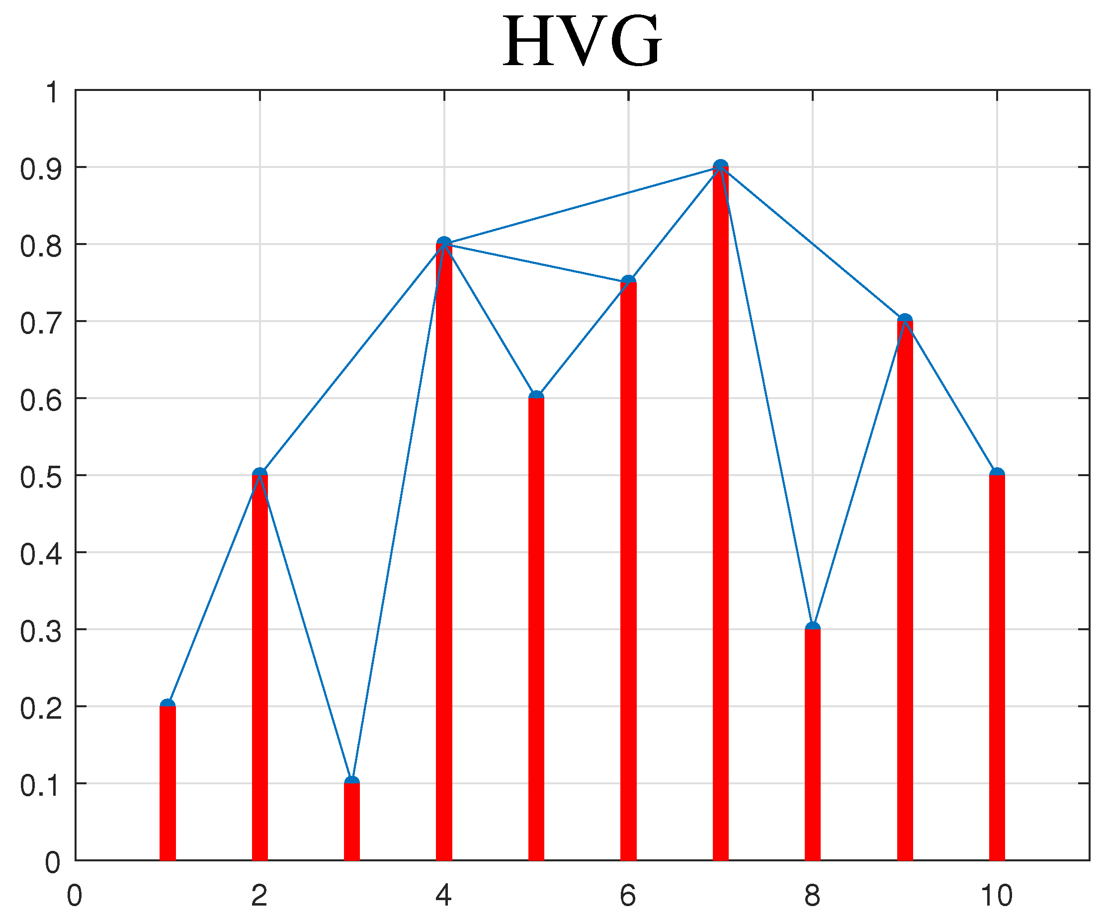
The horizontal visibility graph algorithm was also proposed by Lacasa et al. in 2009 [11]. In this algorithm, two data points are connected by an edge in the network if they can “see” each other horizontally, meaning that the height of any intermediate data bars is less than the heights of the two data bars on either side. The visibility criterion is described as follows: For any ( t c , x c ) between two points ( t a , x a ) and ( t b , x b ) , here t a < t c < t b , if it fulfills relationship:
x a , x b > x c
then there exists a connecting edge between the corresponding two nodes.
To better illustrate this algorithm, a time series consisting of 10 sequentially emitted data points was considered, with the values being 0.2, 0.5, 0.1, 0.8, 0.6, 0.75, 0.9, 0.3, 0.7, and 0.5, respectively. Each data point is abstracted as a column, where the height of each column corresponds to the value of the respective data point. A link is established between two data points if their columns are visually connected horizontally. This representation is shown in Figure 2.

2.3. Limited Penetrable Visibility Graph (LPVG)

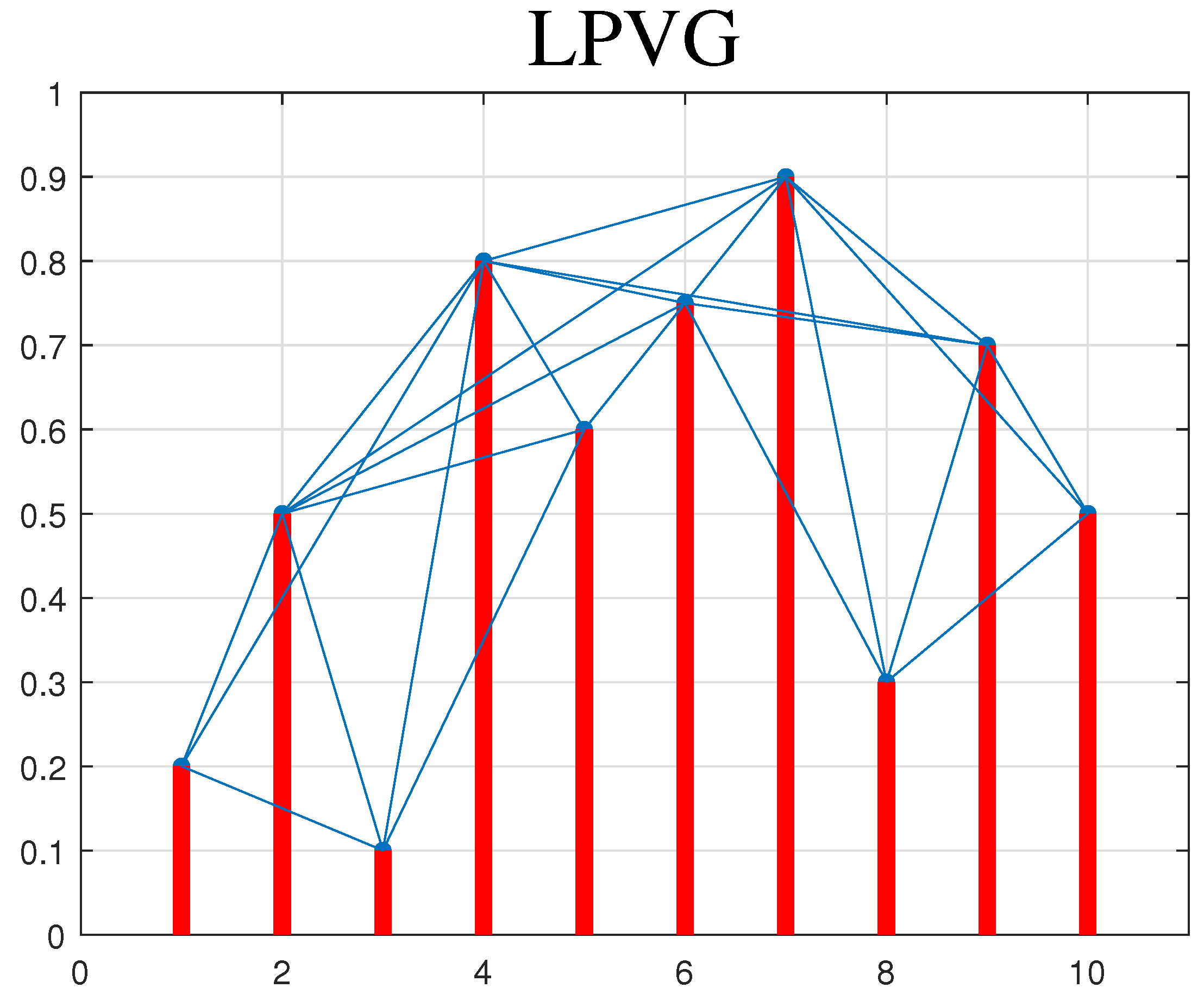
Based on the ideas of the visibility graph (VG), Zhou et al. proposed the Limited Penetrable Visibility Graph (LPVG) method in 2012 [12]. The fundamental idea is to determine the connection between nodes by restricting the obstruction within a limited visibility distance. Specifically, two nodes are considered connected if the number of obstructing bars between them does not exceed a specified visibility distance, L. In other words, even if there are several bars obstructing the line of sight between the nodes, as long as the number of obstructions does not exceed L, the nodes are still regarded as connected.
To further elucidate this algorithm, a time series consisting of 10 sequentially emitted data points is considered, with the values 0.2, 0.5, 0.1, 0.8, 0.6, 0.75, 0.9, 0.3, 0.7, and 0.5, respectively, as depicted in Figure 3.

2.4. Quantile Graphs (QGs)

In 2011, Campanharo et al. proposed quantile graphs (QGs), which map one-dimensional time series of X T to g G on a set of network graphs, where X = { x ( t ) t N ; x ( t ) R } and g = { N , A } are the sets of nodes N (nodes) and arcs A (arcs) [13].
Firstly, a quantile parameter, Q, is defined, which represents the actual number of nodes in the generated component bitmap network. The difference between the maximum and minimum values of the time series X is divided into Q equal parts, denoted as q 1 , q 2 , q 3 , , q Q . Each measured value in X is then assigned to the block corresponding to quantile q i in these Q equal parts. Each quantile q i is assigned to a node n i in the corresponding network. Two nodes, n i and n j , are then connected in the network with a weighted arc, ( n i , n j , w i j ) , where the weight, w i j , of each arc is the transition probability in a Markov model estimated from the aggregate time series [14].
The weight, w i j k , is determined by the evolutionary correlation between the time series measured values x ( t ) and x ( t + k ) , which belong to the block indices q i and q j , where t = 1 , 2 , , T , k = 1 , 2 , , k max < T . The weight, w i j k , is evolved by the k step only. The probability of the transition between x ( t ) in block i and x ( t + k ) in block j determines the weight, such that larger weights between two nodes result in thicker lines in the associated network. The QG method exhibits low sensitivity to the selection of Q, where Q T is assumed.
After performing l = L random jumps of lengths δ l , k ( i , j ) = | i j | , the calculation of the average jump length Δ ( k ) can be described by the following equation:
Δ ( k ) = 1 L l = 1 L δ l , k ( i , j )
where i , j = 1 , 2 , , Q is a node index indicator defined by W k .
The average jump length, Δ ( k ) , can also be obtained directly from the Markov state transition matrix W k , which is especially suitable for the case of many network nodes. At this time, the specific calculation formula of Δ ( k ) is as follows:
Δ ( k ) = 1 Q tr P W k T
where W k T is the transpose of the state transition matrix, P is the matrix element defined by p = p i , j Q × Q , and  tr ( · ) represents the matrix trace operation [14].
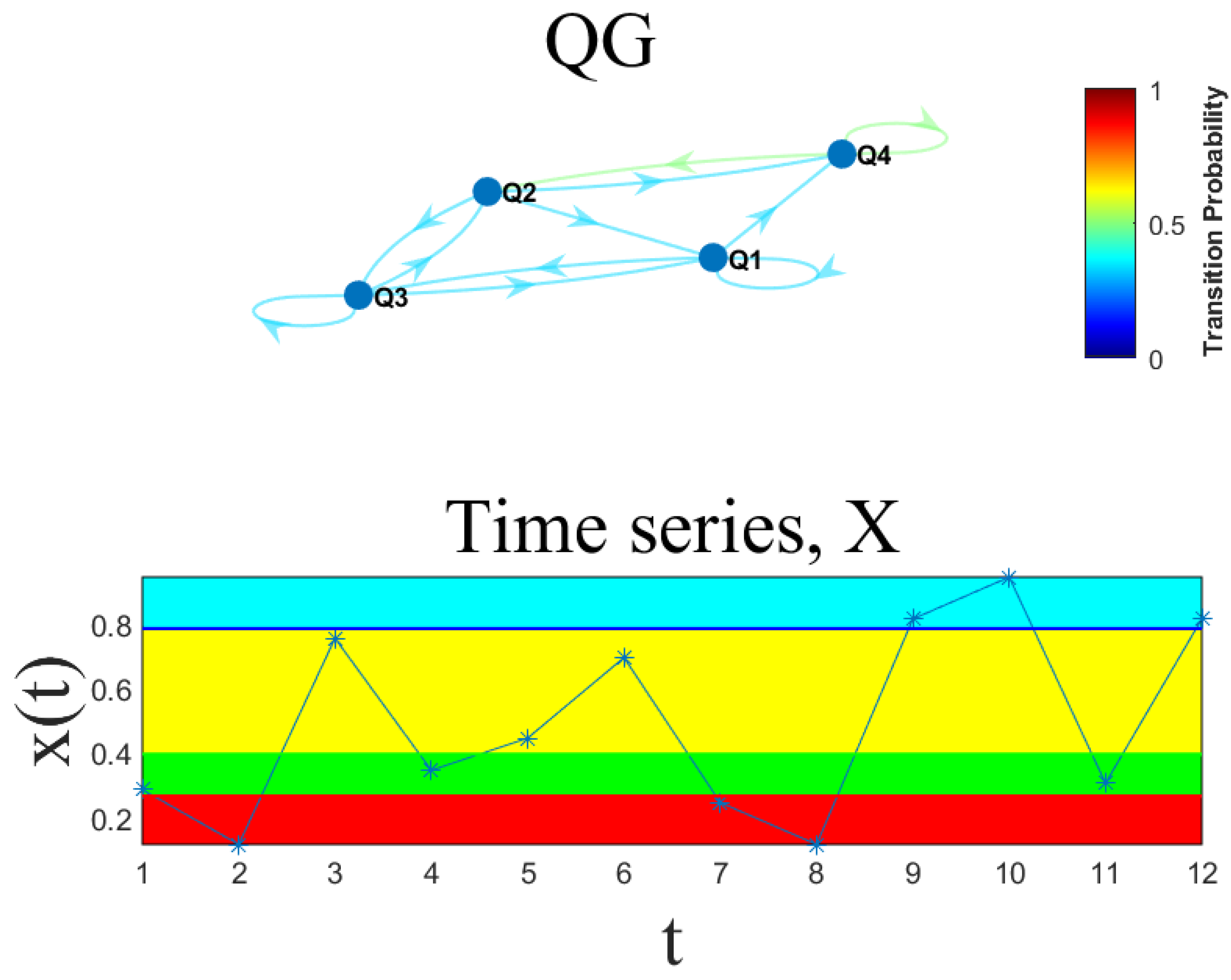
To better illustrate this algorithm, we provide a time series consisting of 12 points: 0.29, 0.12, 0.76, 0.35, 0.45, 0.7, 0.25, 0.12, 0.82, 0.95, 0.31, and 0.82. An example of this algorithm with T = 12 , Q = 4 , k = 1 is shown in Figure 4.

2.5. Modified Frequency Degree Method (MFDM)

The order of time series and reproduction are two key attributes in time series analysis. In order to better mine the features of the original time series and transform the time series into a network, Li et al. proposed a frequency degree algorithm [15]. The idea of the frequency degree algorithm is that the data with high reproduction frequency will correspond to the value with magnanimity. Specifically, the frequency degree algorithm divides the time series into equidistant intervals according to the amplitude and then connects each node to its nearest left and right neighbors in time order, and then it fully connects the nodes located in the same interval. This method can preserve the amplitude and time information of the original time series.
In 2025, Niu and Liu proposed a modified frequency degree method [16] that further considers the positional information of the time series data points. Specifically, let N be the length of the time series and Q be the parameter to be input. We consider two cases: If N is divisible by Q, then the data points of the time series are evenly distributed into Q intervals. If N is not divisible by Q, then the data points of the time series are divided into Q + 1 intervals.
The N divisible Q case: If N is evenly divided by Q, these data points will be bisected into these intervals, d = N Q , the time series will be sorted from smallest to largest, and the time series data points will be divided according to [d: d: N]; then, the data points in the same interval will be connected with its two nearest neighbors, and the data points in the same interval will be fully connected. For convenience of illustration, we present a schematic diagram of the modified frequency degree method under the condition that it can be evenly divided in Figure 5.
As shown in Figure 5, we select the time series 3, 6, 1.5, 9, 7, 8, 5, and 6, and Q = 4 with a length of 8. Firstly, the time series is sorted, and the points on the boundary line all belong to the following smaller interval. The data points are then divided into four intervals. The first-order time series is 1.5, 3, 5, 6, 6, 7, 8, and 9, and then the corresponding position of the time series is found according to d = 8 4 = 2 ; that is, [2:2:8] = 2, 4, 6, and 8 corresponds to the interval limits, so the divided interval ranges are ( , 3 ] , ( 3 , 6 ] , ( 6 , 7 ] , ( 7 , 9 ] . So, the time series is 3, 6, 1.5, 9, 7, 8, 5, and 6, and the corresponding interval is [1, 2, 1, 4, 3, 4, 2, and 2]. Next, each data point is connected to its two nearest neighbors, and then the data points that are in the same interval are fully connected.
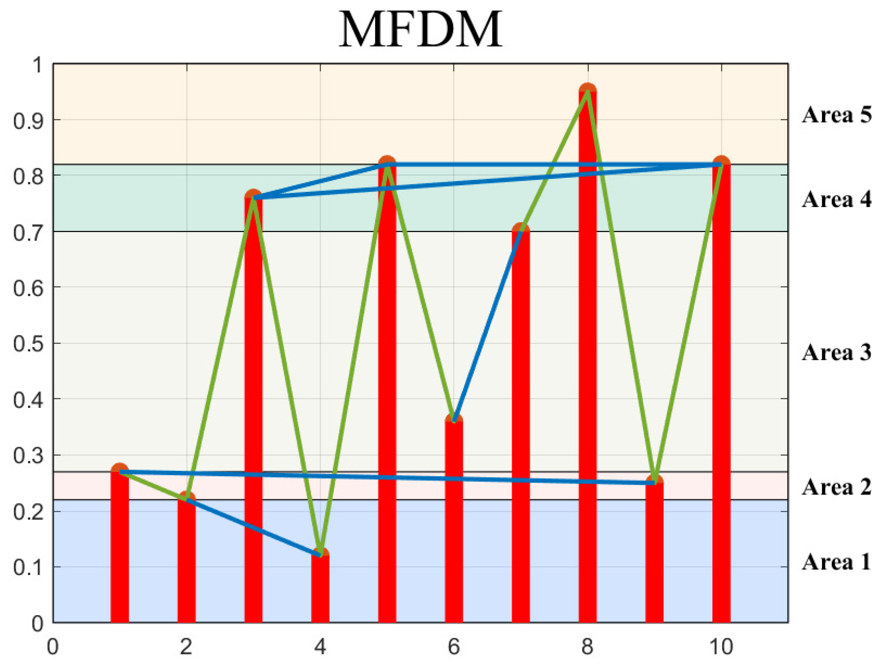
If N does not divide Q exactly: If N does not divide Q exactly, these data points will be divided into Q + 1 intervals. We denote d = N Q , and the time series will be sorted from smallest to largest. The time series data points will be divided according to d : d : N , and then the data points located in the same interval will be fully connected after each data point is connected with its two nearest neighbors. In Figure 6, we provide a schematic diagram of the modified frequency degree mapping algorithm when it is not evenly divided.
As shown in Figure 6, we consider a time series of length 10: 0.27, 0.22, 0.76, 0.12, 0.82, 0.36, 0.7, 0.95, 0.25, and 0.82, with Q = 4 . First, we sort the time series in ascending order: 0.12, 0.22, 0.25, 0.27, 0.36, 0.7, 0.76, 0.82, 0.82, and 0.95. Next, compute d as follows: d = N Q = 10 4 = 2 . Then, we divide the time series data points into intervals based on [ d : d : N ] , i.e., [2:2:10] = 2, 4, 6, 8, and 10. The intervals are as follows: ( , 0.22 ] , (0.22, 0.27], (0.27, 0.7], (0.7, 0.82], and (0.82, 0.95]. Thus, the time series of 0.27, 0.22, 0.76, 0.12, 0.82, 0.36, 0.7, 0.95, 0.25, and 0.82, corresponds to the following interval indices: [2, 1, 4, 1, 4, 3, 3, 5, 2, 4]. Finally, we connect each data point to its two nearest neighbors, and we fully connect all data points within the same interval.
According to the literature [15], when the length range of a given time series is 1000 to 10,000, it may be appropriate to select a Q equal to 128 or 256. Therefore, Q = 128 is selected in this paper.

3. Main Framework, Dataset, and Feature Extraction Overview

3.1. Main Framework

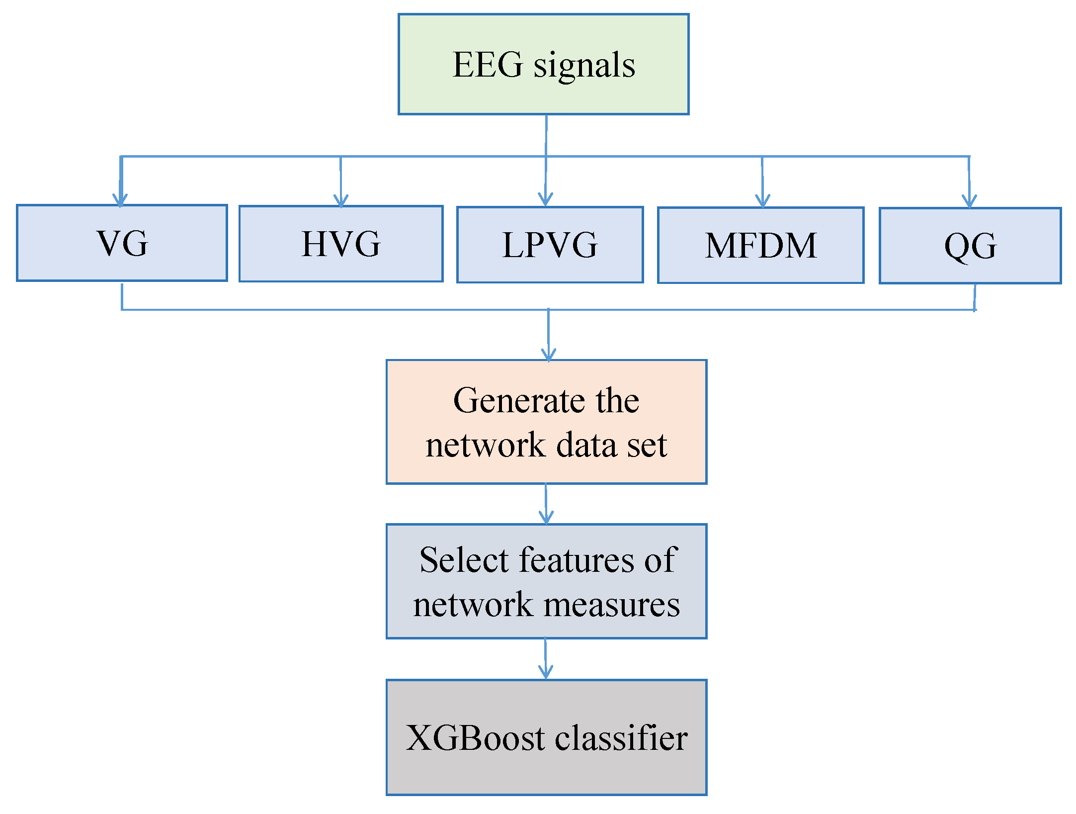
This paper first converts EEG signals into corresponding associated networks using five different methods: VG, HVG, LPVG, MFDM, and QG. For each algorithm, the related network measures of the associated networks are all firstly calculated. Then, features with a significance level greater than 0.05 are filtered out using ANOVA. The remaining network features are concatenated into a vector and input into the XGBoost classifier for classification. The main framework process of this paper is shown in Figure 7.

3.2. Dataset Used in Numerical Experiments

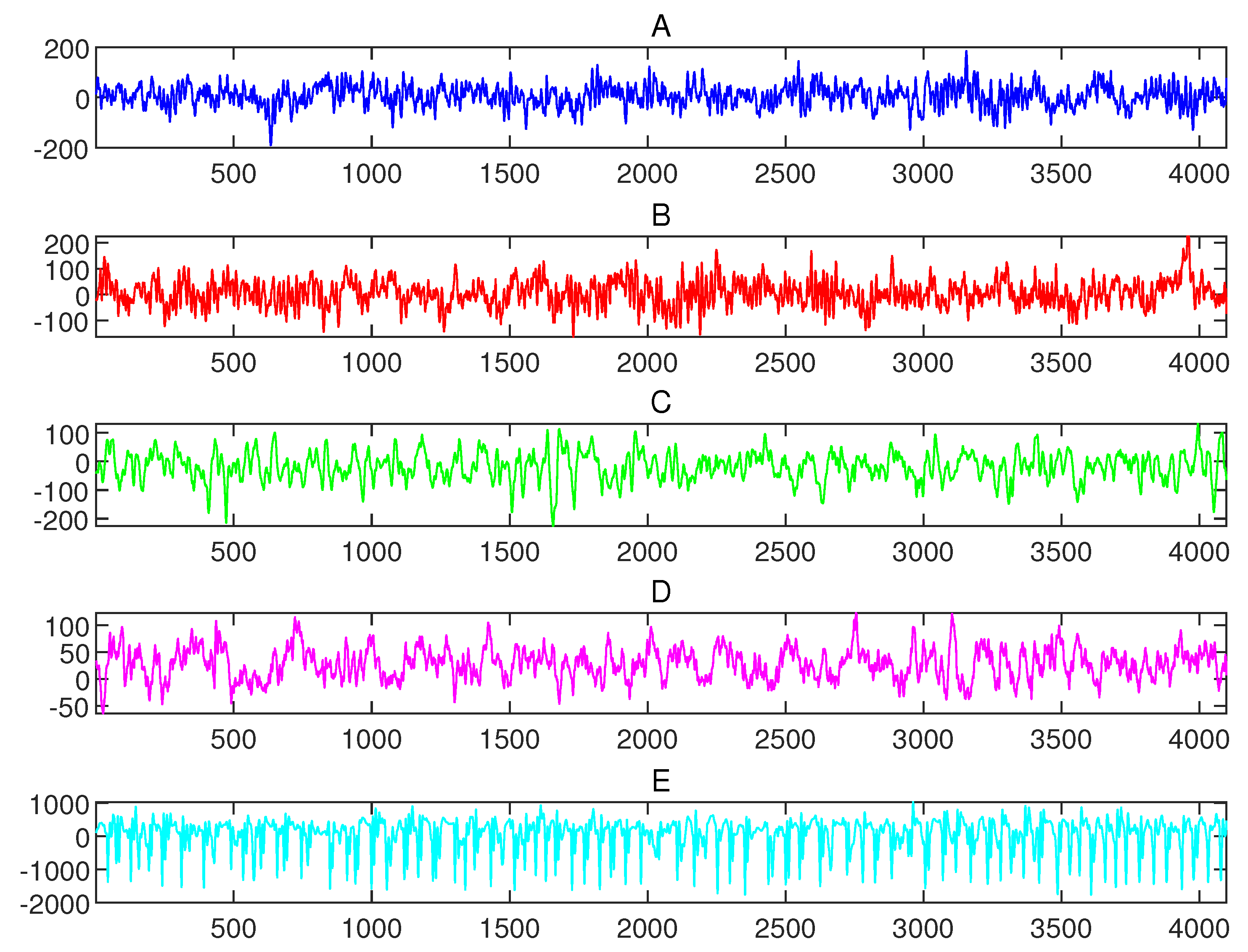
In this study, we utilize the artifact-free EEG database provided by the University of Bonn, which is freely available online [17]. This database has been widely used for EEG feature extraction and classification in the literature [18]. Our dataset comprises five distinct sets, labeled A, B, C, D, and E. Each set contains 100 single-channel EEG segments, each segment lasting 23.6 s and sampled at a rate of 173.61 H z . Sets A and B consist of surface EEG recordings from healthy, awake volunteers, with Set A containing recordings taken while the volunteers had their eyes open and Set B containing recordings taken with their eyes closed. Sets C and D contain intracranial EEG signals from epileptic patients recorded during seizure-free intervals, with Set C containing recordings from the hippocampal formation in the opposite hemisphere of the brain and Set D containing recordings from the epileptogenic zone. Set E includes intracranial EEG signals recorded at sites exhibiting ictal activity, representing seizure activity. Figure 8 illustrates sample EEG segments from sets A, B, C, D, and E. There are five data subsets, each containing 100 brain telecom number segments and 4097 data points. The data have been filtered according to related literature published in the last several decades (i.e., we chose to filter broadband in 0.53–40 H z . This range covers most of the EEG frequency components associated with cognitive activity, such as α waves (8–12 H z ) and β waves (13–30 H z )), and the specific state diagram of different types of EEG signals can be seen in Figure 8.

3.3. Feature Extraction

In this process, extracting features from EEG signals is crucial, as they carry different information, depending on whether the subject is healthy or epileptic and whether they are in a seizure or non-seizure state. Initially, EEG time series are transformed into associated networks using various methods. The adjacency matrix of each network is stored, and the average degree, average clustering coefficient, density, network diameter, global efficiency, and average path length are calculated for networks under five different algorithms: the VG, the HVG, the LPVG, MFDM, and the QG [19,20,21]. Additionally, the average jump length Δ is computed for networks under the QG algorithm [13]. The network measures obtained from each algorithm are then standardized. Subsequently, an analysis of variance (ANOVA) is used to filter out columns with significance levels greater than 0.05 . In statistics, 0.05 is often used as a standard threshold to determine whether a result is statistically significant. Choosing 0.05 as the significance level means that, if the p-value of a feature is less than 0.05 , it is considered that the feature has a significant impact on the classification task. On the contrary, it is considered that the influence is not significant. This selection was based on balancing considerations in statistical conventions and practical applications, aiming to include as many features useful for classification as possible while controlling for false positive rates. The strength of ANOVA is its simplicity and intuitiveness, which directly assesses the relationship between features and labels and is effective in many cases.
As shown in Algorithm 1, the ANOVA feature concatenation method selects significant features based on their p-values. This method is effective in reducing the dimensionality of the dataset by retaining only those features that have a statistically significant impact on the target variable.
Algorithm 1 ANOVA feature concatenation
1:
Input: Dataset X R m × n , labels Y R m , significance threshold α = 0.05
2:
Output: Concatenated feature set X selected
3:
Initialize empty list selected _ features
4:
for each feature f i in X do
5:
      Perform ANOVA to compute p-value p i for feature f i
6:
      if  p i < α then
7:
           Append feature f i to selected _ features
8:
      end if
9:
end for
10:
Concatenate the selected features into a new set, X selected
11:
Return  X selected
The remaining network measures for each algorithm are concatenated into a single vector. These vectors are combined to form a feature matrix, which is then used as input for traditional classification machine learning models.
Through an analysis of variance, we filter out the network diameter feature for both VG and LPVG. The final selected features for each algorithm are listed as follows:
  • VG: average degree ( α V G ); the maximum degree( M V G ); average clustering coefficient ( C V G ); density: ( ρ V G ); global efficiency: ( G V G ); and average path length: ( L V G ).
  • HVG: average degree ( α H V G ); the maximum degree ( M H V G ); average clustering coefficient ( C H V G ); density: ( ρ H V G ); global efficiency: ( G H V G ); network diameter ( D H V G ); and average path length: ( L H V G ).
  • LPVG: average degree ( α L P V G ); the maximum degree ( M L P V G ); average clustering coefficient ( C L P V G ); density: ( ρ L P V G ); global efficiency: ( G L P V G ); and average path length: ( L L P V G ).
  • MFDM: average degree ( α M F D M ); the maximum degree ( M M F D M ); average clustering coefficient ( C M F D M ); density: ( ρ M F D M ); global efficiency: ( G M F D M ); network diameter ( D M F D M ); average path length: ( L M F D M ).
  • QG: and average jump length ( Δ ).
Remark 1.
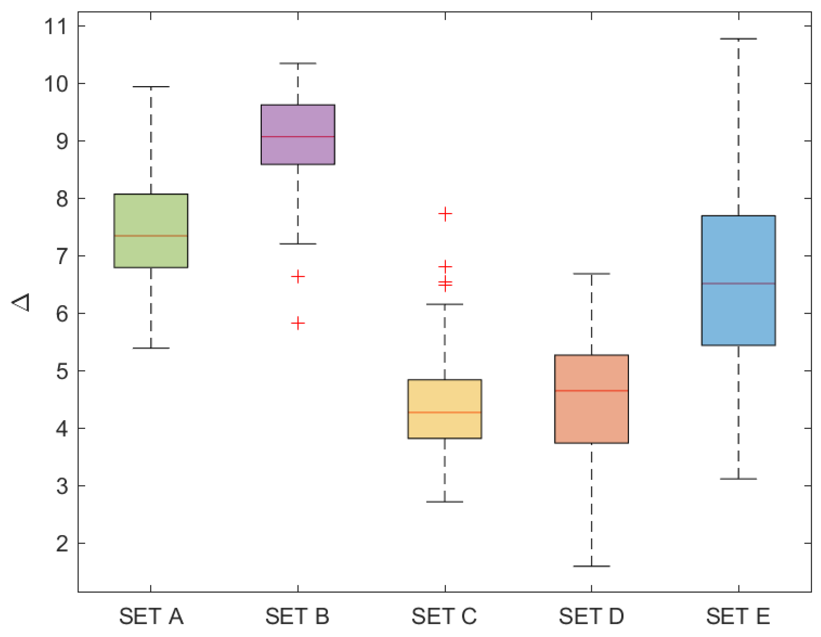
For the QG algorithm, the most representative feature, namely the average jump length, is selected. As suggested by the literature [4], when Q = 30 and k = 4 , significant differentiation is observed within the dataset. Hence, we chose Q = 30 and k = 4 . The corresponding box plot is presented in Figure 9.
The feature vector V EEG signals is constructed using multiple-measures composited strategies and is typically described as follows:
V EEG signals = α VG , , L VG , α HVG , , L LPVG , α MFDM , , L MFDM , Δ QG
Therefore, the feature vector V EEG signals is composed of twenty-seven network measures used for subsequent classification tasks.

3.4. Model Evaluation Index

In order to facilitate the evaluation in the following article, we first give some definitions of evaluation indicators and cross-validation listed as below. Related indicators are introduced in the literature [22,23,24,25].
Accuracy: Accuracy is the ratio of the number of correct predictions to the total number of predictions. It reflects how often the classifier is correct across all classes.
Balanced accuracy: Balanced accuracy measures model performance on imbalanced datasets. It is the average of the recall rates for each class, providing a more accurate reflection of the model’s ability to recognize the minority class. Balanced accuracy values range from 0 to 1, with 1 being the best.
F 1 -Score: The F1-score is the harmonic mean of precision and recall, representing the overall effectiveness of the model in classification tasks. It balances the trade-off between precision and recall, especially in cases of class imbalance.
Specificity: Specificity measures the proportion of actual negatives correctly identified as negatives. In multiclass classification, it is calculated for each class as the proportion of actual non-class samples correctly identified as non-class.
True negatives (TNs): true negatives for class i are the count of actual non-class i samples correctly predicted as non-class i.
False positives (FPs): false positives for class i are the count of actual non-class i samples incorrectly predicted as class i.
Precision: precision is the proportion of predicted positive samples that are actually positive, reflecting the accuracy of positive predictions.
Recall: recall is the proportion of actual positive samples correctly predicted as positive, indicating the model’s ability to identify relevant positive samples.
Matthews correlation coefficient (MCC): MCC is a balanced classification metric ranging from [ 1 , 1 ] , measuring the quality of binary classifications by considering true and false positives and negatives.
Cohen’s kappa: Cohen’s kappa assesses agreement between the classifier and a random classifier, adjusting for chance agreement for a nuanced evaluation.
Hamming loss: Hamming loss represents the proportion of incorrectly classified samples, measuring the average number of misclassified labels.
Jaccard index: the Jaccard index, or intersection over union (IoU), evaluates classifier accuracy by comparing the intersection and union of predicted and actual sets.
Cross-validation: Cross-validation involves dividing the dataset into k subsets, using k 1 subsets for training and 1 for testing in each iteration. This process is repeated k times, with each subset serving as the test set once, and the results are aggregated for final evaluation.

4. Classification Effect on the Dataset

In this paper, we use the XGBoost classifier (i.e., XGBClassifier) to classify EEG data and evaluate our method’s performance. XGBoost (eXtreme Gradient Boosting) is an enhanced machine learning model suitable for regression, classification, and ranking problems. This model is based on the gradient boosting algorithm, which improves the overall predictive performance by iteratively building and combining multiple weak classifiers [26]. Specifically, we first normalize the feature data so that the mean is 0 and the standard deviation is 1. Then, we set the parameters of the XGBoost classifier. After that, we use stratified cross-validation (StratifiedKFold) to divide the data into ten folds, with nine folds used for training and one fold used for validation. The performance of the XGBoost classifier on the given EEG dataset is evaluated through 10-fold cross-validation. We conduct experiments using our framework on both binary classification and five-class classification tasks. For each individual method, the final selected network features are as follows: For VG, HVG, LPVG, and MFDM, the following seven network measures were selected: average degree, maximum degree, average clustering coefficient, network density, network diameter, global efficiency, and average path length. For QG, the average jump length was selected.
Our method involves concatenating the network measures obtained from each of the aforementioned algorithms into a long vector. We then use ANOVA to assess the relationship between each feature and the labels, selecting the features that have a significant impact on the classification task. The p-value for each feature indicates whether there is a significant difference in the mean across different categories. If the p-value is greater than 0.05 , it suggests that the feature does not have a significant impact on the classification task, and thus, the feature is discarded. The p-value of the computed features are shown in Table 1.
After calculation, we find that the p-value of the network diameter feature under the VG and LPVG methods are 0.54 and 0.81 , respectively, so we filter out the network diameter feature for both the VG and LPVG methods. Additionally, we observe that removing any feature would lead to a decrease in classification accuracy, negatively impacting the classification task. Therefore, we select these 27 features as the feature vector, as they can more comprehensively capture the intrinsic characteristics of the signal.
Remark 2.
A 27-dimensional feature vector filtered via an ANOVA reduces redundancy while retaining discriminative power. The average jump length, Δ Q G , from Q G contributes most significantly to class separation.

4.1. Classification Effect on Binary Classification Dataset

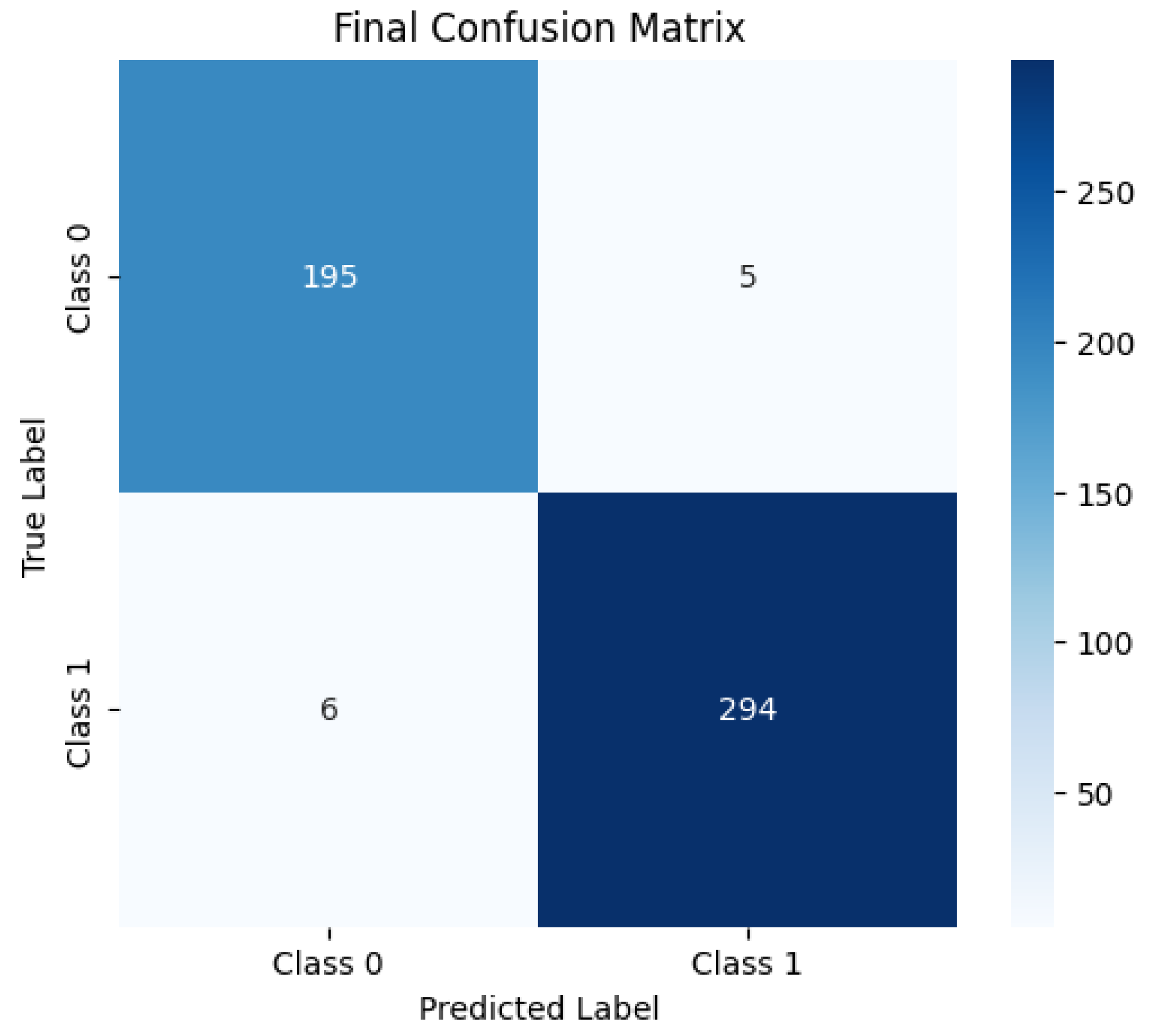
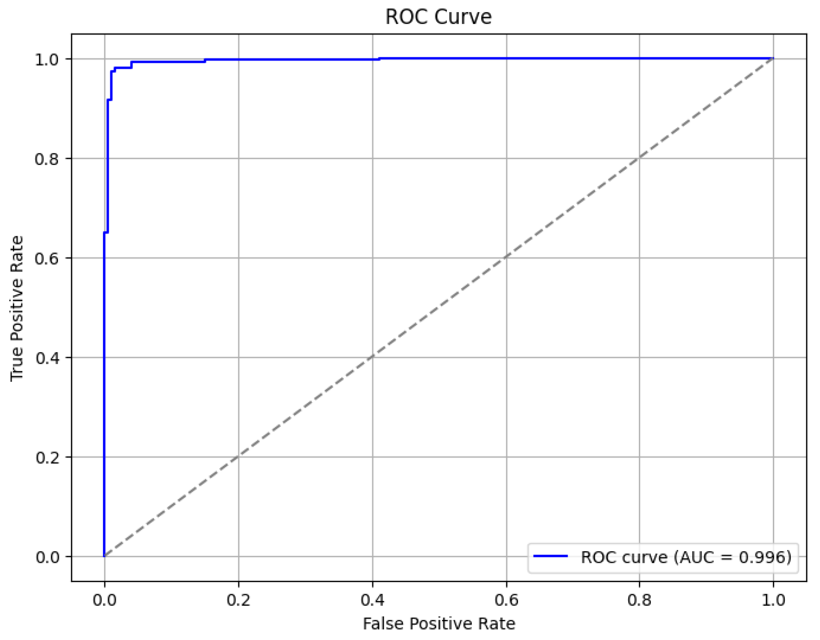
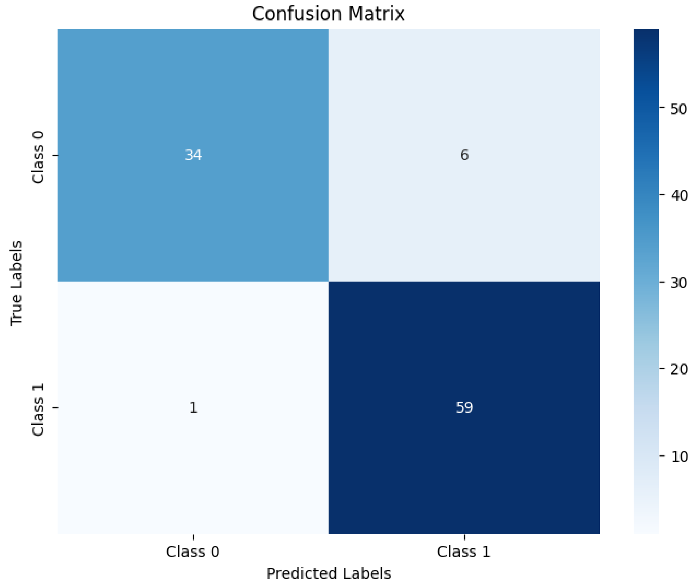
XGBoost has achieved remarkable results in many fields, so we want to use this model to classify epilepsy. In epilepsy detection, a high-precision model can distinguish between epilepsy patients and healthy people, helping doctors quickly and accurately determine whether patients have specific diseases and thereby accelerating the treatment process. Through automated and intelligent binary classification, decision-making efficiency can be significantly improved, and the time and cost of manual judgment can be reduced. Therefore, we first evaluated the effect of the framework proposed in this article on binary classification tasks. We first performed a binary classification by grouping A (healthy, eyes open) and B (healthy, eyes closed) as one category, labeled as Class 1. C (epileptic, opposite zone), D (epileptic, epileptogenic zone), and E (epileptic, seizure) were grouped together as another category, labeled as Class 2. The classification was performed using the XGBoost model. The performance of the model is summarized in Table 2, which presents several evaluation metrics. The confusion matrix diagram and ROC curve of the XGBoost model on the binary classification task are plotted in Figure 10 and Figure 11, respectively.
Although the individual classification algorithms do not exhibit high accuracy, the performance improves significantly after applying the feature concatenation method based on ANOVA. The results demonstrate that our feature extraction framework, when coupled with the XGBoost model, yields excellent performance across various evaluation metrics. The classification performance of various algorithms was compared, and the results show that our method outperforms others on multiple evaluation metrics. The balanced accuracy achieved was 0.978 , indicating that the model has strong performance across both classes. The specificity reached 97.5 % , demonstrating that the model is highly effective in identifying non-positive samples. The F1 score of 0.982 further emphasizes that the model maintains a good balance between precision and recall, while the precision value of 0.983 indicates that the model is highly accurate in predicting positive cases. The recall rate of 0.980 reflects the model’s ability to correctly identify positive samples. Furthermore, the Matthews correlation coefficient (MCC) and Cohen’s kappa coefficient, both at 0.954 , suggest that the model’s predictions are significantly better than random chance. The Hamming loss of 0.020 indicates that only 2 % of the samples were misclassified, while the Jaccard index of 0.964 confirms a high level of agreement between predicted and actual results. These findings highlight the effectiveness and robustness of our feature extraction framework when used in conjunction with the XGBoost model. To further evaluate the impact of different classifiers on classification results, we performed experiments using MATLAB’s Classification Learner tool (after sorting). The results are summarized in Table 3, which presents the performance of various classifiers in binary classification tasks. To make it easier to see which are the top 10 models of the Matlab2023b classification toolbox in the binary classification task, we visualized them in Figure 12. We compared the method in this paper with the popular EEG classification model CNN method based on deep learning, and from Figure 13, we found that the test set accuracy of the CNN method on the binary classification task was 0.93, which was not as high as the accuracy of the method proposed in this paper. This can illustrate the effectiveness of our method. The confusion matrix under the CNN method is shown in Figure 14. Therefore, our framework performs well across all indicators of the binary classification tasks.

4.2. Classification Effect on Five Classification Datasets

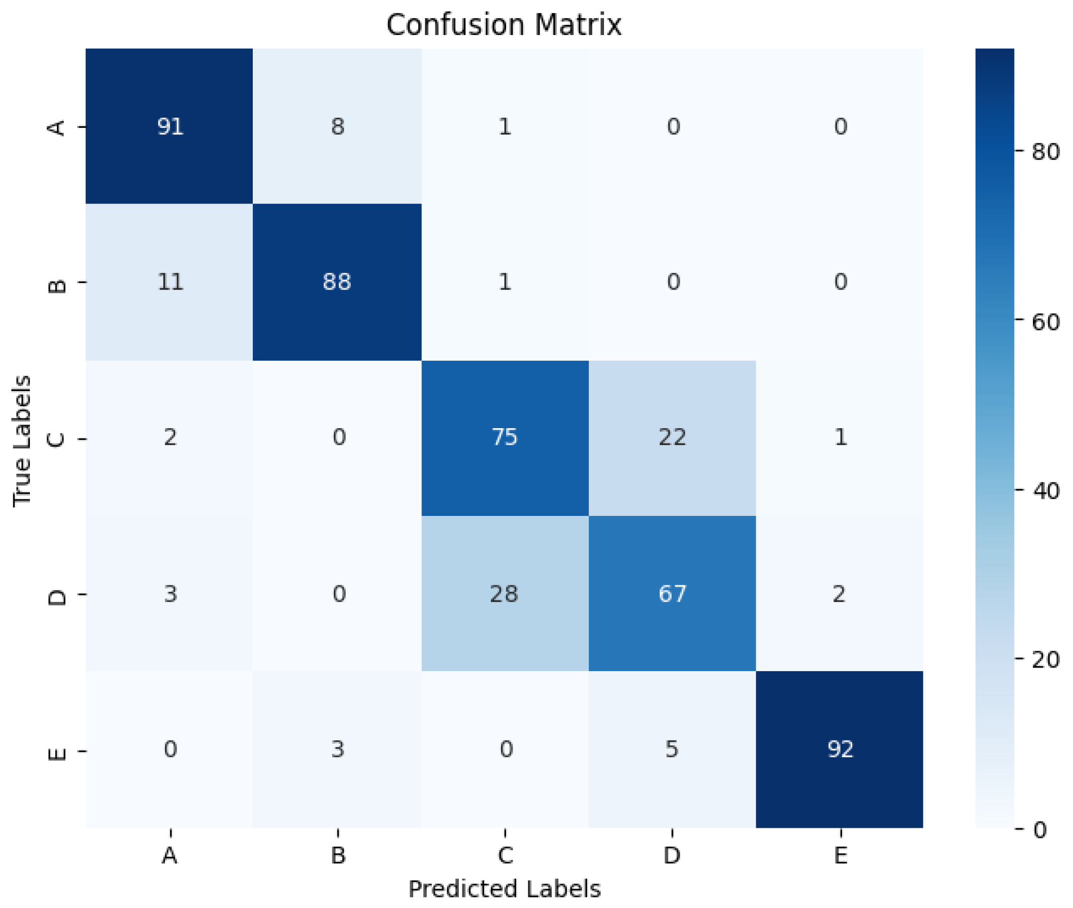
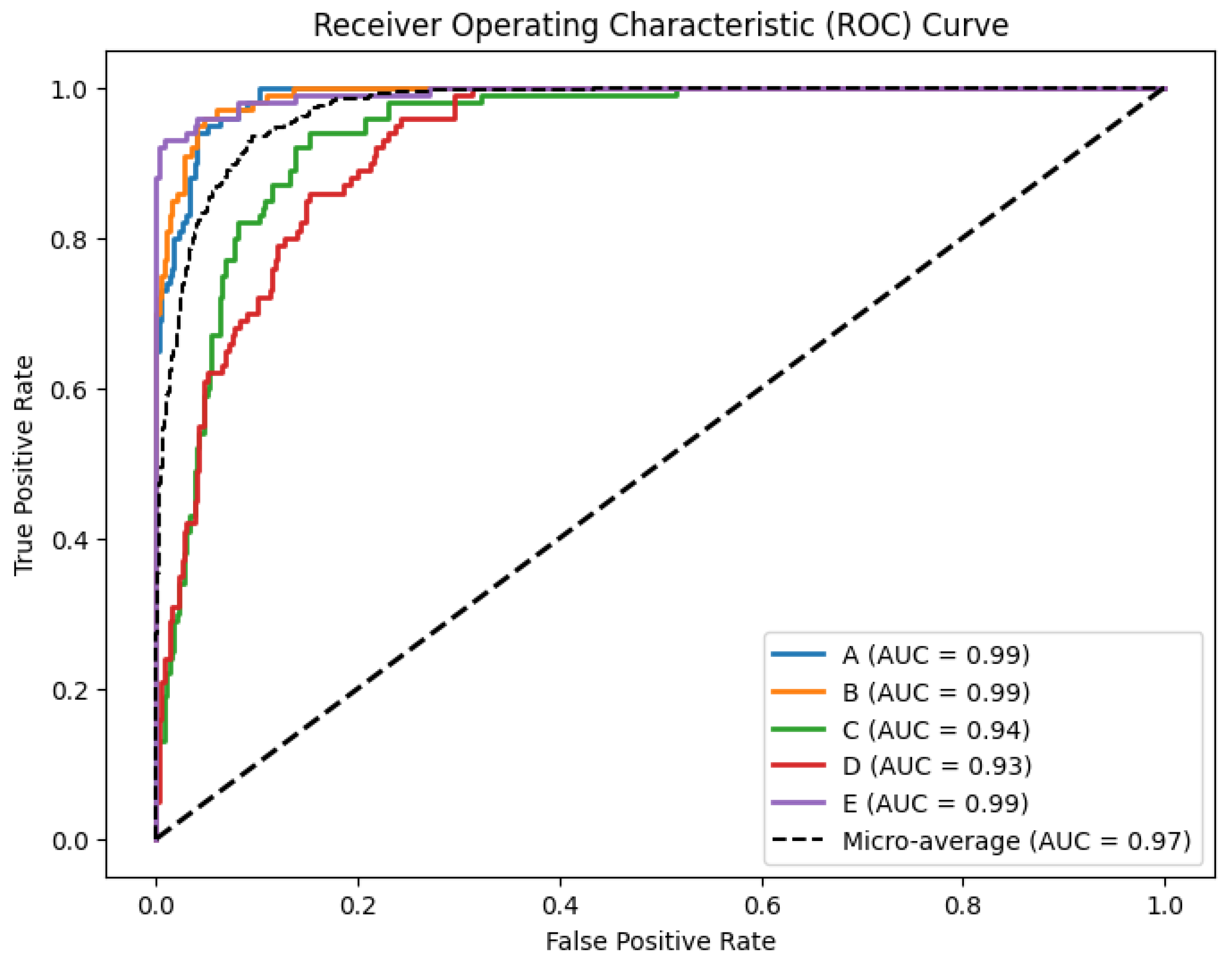
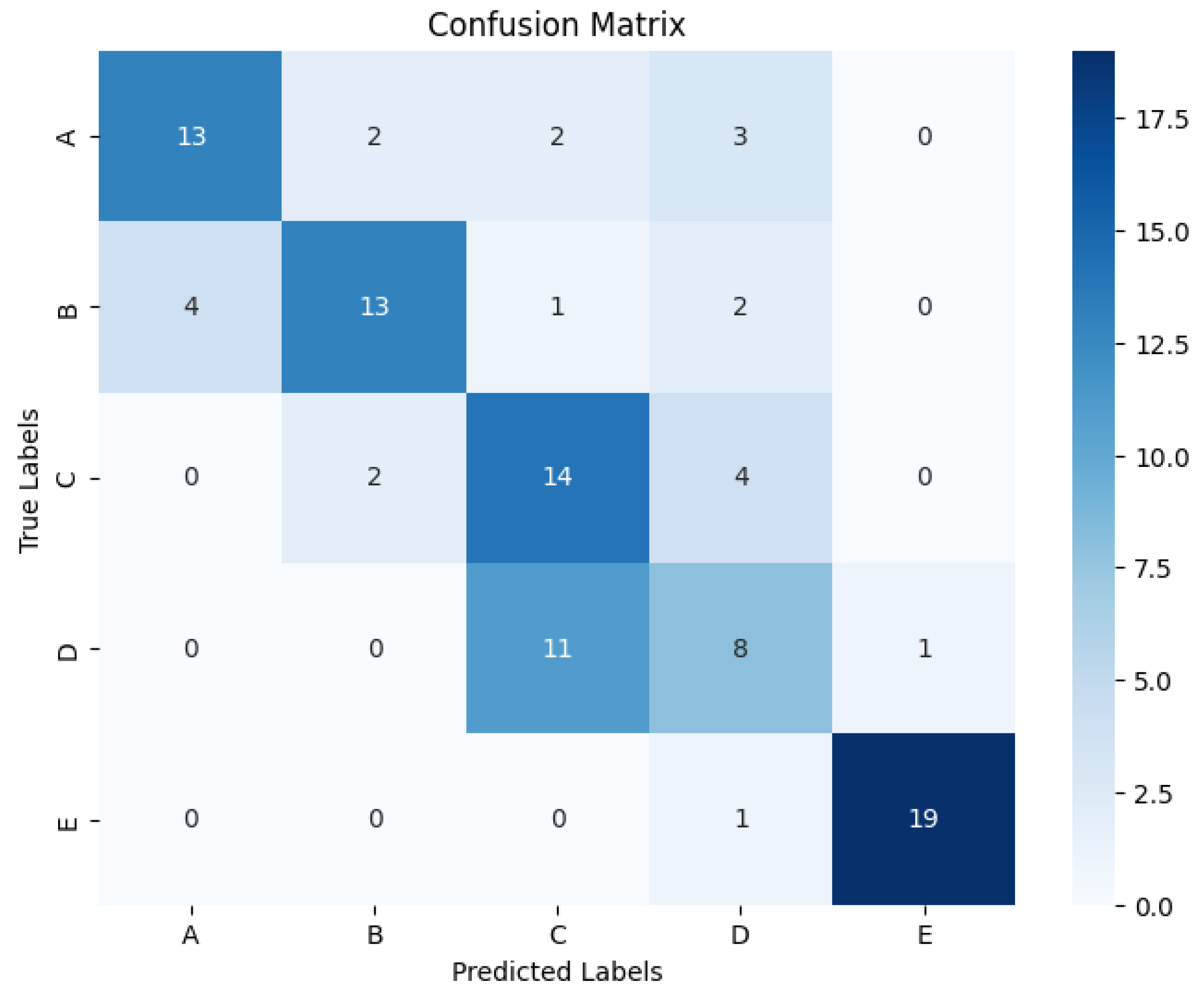
In this article, the five-category classification of EEG signals can more finely distinguish between healthy states and different states of epilepsy. The five-category classification task helps doctors make more detailed divisions of patients’ disease states, thereby formulating more personalized treatment plans. In epilepsy treatment, understanding the patient’s specific seizure type and brain area activity is crucial to choosing appropriate drugs and surgical strategies. Through the five-category classification, we can more deeply analyze the differences and connections between different disease states and provide data support for the exploration of disease mechanisms and innovation of treatment methods. Therefore, the five-class classification was then performed. The evaluation metrics for both the single-method XGBoost model and our method obtained using Python are as follows in Table 4. The confusion matrix diagram and ROC curve of the XGBoost model on the five classification tasks are plotted in Figure 15 and Figure 16, respectively.
Although the classification accuracy of individual algorithms is relatively low, the performance metrics for the five-class classification are significantly improved after applying the feature concatenation method based on ANOVA. It is observed that our feature extraction framework performs well across various performance indicators when classified with the XGBoost model. The balanced accuracy is 0.824, demonstrating that the model performs consistently across all classes, with an overall accuracy of 82.4%. The specificity reaches 95.6%, indicating the model’s strong ability to correctly identify non-target samples for each class. The F 1 score is also 0.823, highlighting a good balance between precision and recall. Both the accuracy and recall rates stand at 0.824, showing the model’s reliability in predicting positive samples and effectively identifying most of the actually positive cases. The precision value of 0.823 indicates that the model is highly accurate in predicting positive cases. The Matthews correlation coefficient (MCC) and Cohen’s Kappa coefficient are both 0.780, suggesting that the model’s prediction quality is significantly better than random guessing. The Hamming loss is 0.176, meaning 17.6% of the samples were misclassified, while the Jaccard index is 0.715, indicating a 71.5% similarity between the predicted and actual results.
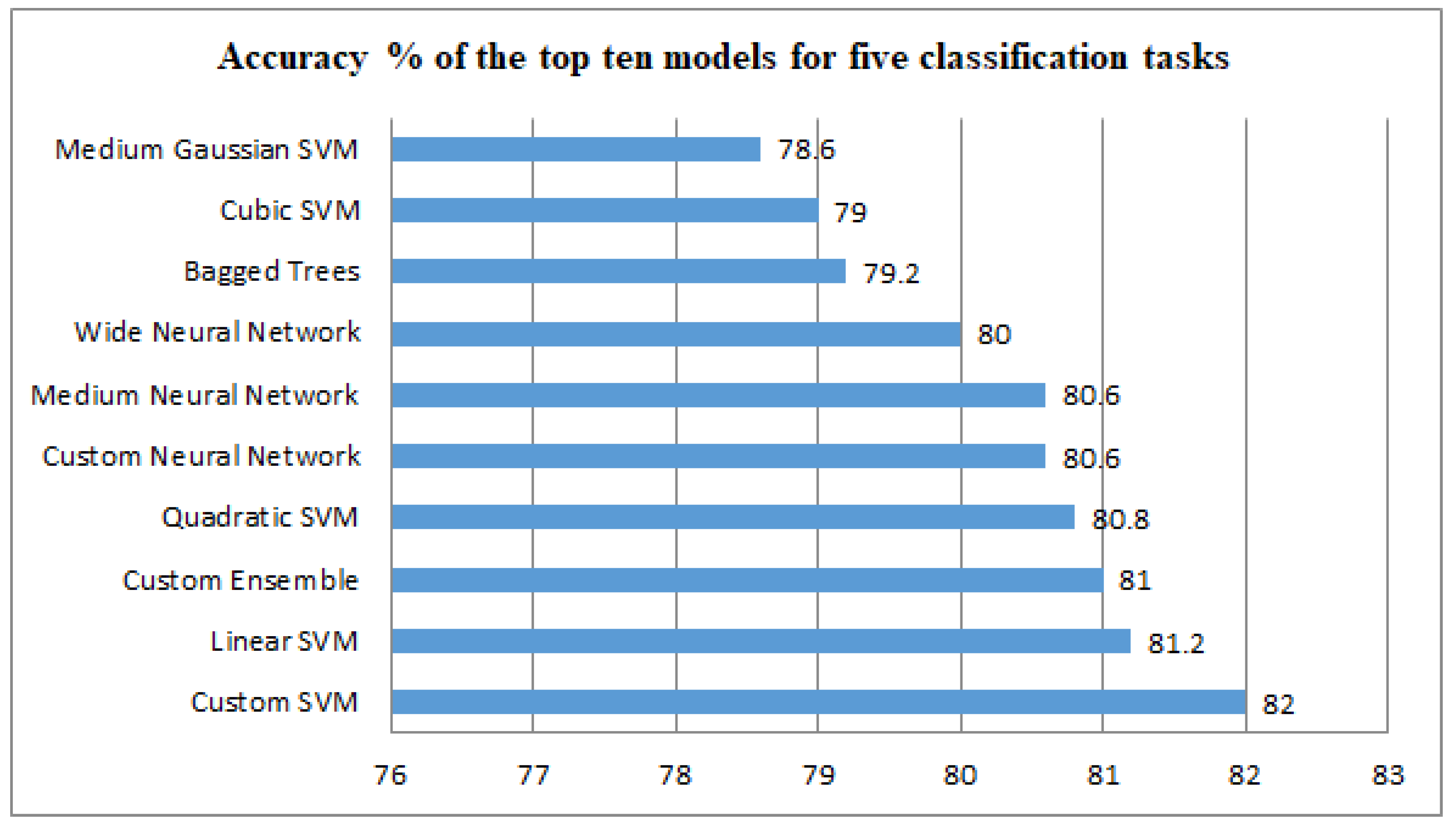
In summary, the XGBoost model demonstrates excellent performance across multiple metrics, proving to be both robust and effective on this dataset. A comparison of other machine learning methods using MATLAB’s Classification Learner is presented as follows (after sorting) in Table 5. To make it easier to see which are the top 10 models of the Matlab R2023b classification toolbox in the five classification tasks, we have made a visualization in Figure 17. Therefore, our framework performs well on all indicators of the five classification tasks.
We compared the method in this paper with the popular EEG classification model CNN method based on deep learning, and from Figure 18, we found that the test set accuracy of the CNN method on the five classification task was 0.67, which was not as high as the accuracy of the method proposed in this paper. This can illustrate the effectiveness of our method. The confusion matrix under the CNN method is shown in Figure 19. Therefore, our framework performs well across all indicators of the five classification tasks.
From Table 5, it can be seen that, using XGBoost, the framework performs well across various metrics in the five-class classification task, with the highest classification accuracy achieved.

5. Conclusions and Outlook

In this paper, a multi-network feature-fusion framework integrating five complex network transformation methods (the VG, the HVG, the LPVG, MFDM, and the QG) has been proposed for epileptic EEG classification. The VG and the HVG capture local temporal patterns, the QG quantifies long-range transition properties, and MFDM enhances sensitivity to amplitude distributions. This fusion overcomes the limitations of single-algorithm approaches. The experimental results demonstrate that the proposed framework achieves an accuracy of 97.8 % and a specificity of 97.5 % in binary classification tasks, with a balanced accuracy of 97.8 % and an F1 score of 0.982 . These results highlight the model’s ability to effectively distinguish between healthy and epileptic EEG signals. The Matthews correlation coefficient and Cohen’s kappa coefficient, both at 0.954 , further confirm the model’s superior predictive quality compared to random guessing. In the more complex five-class classification task, the framework achieves an accuracy of 82.4 % and a specificity of 95.6 % . The balanced accuracy of 82.4 % and an F1 score of 0.823 indicate that the model maintains a good balance between precision and recall across multiple classes. The Matthews correlation coefficient and Cohen’s Kappa coefficient, both at 0.780 , demonstrate the model’s effectiveness in handling multi-class classification. The proposed framework exhibits robust performance in both binary and five-class classification tasks, demonstrating high accuracy and specificity and thereby validating its effectiveness.
The framework eliminates the need for complex signal preprocessing or deep learning infrastructure, making it well-suited for resource-constrained medical environments while providing real-time diagnostic support for clinicians. Additionally, its efficient implementation reduces computational demands. However, there are also some limitations. For example, the amount of data in this paper is not large, and the data are only verified on classic datasets. Future studies will expand the experiment by incorporating multi-center clinical data (such as the CHB-MIT dataset). Since the method of this paper requires converting the time series into a network before calculating the feature classification, it is more applicable to time series with a length of less than 10 , 000 . The framework of this paper can be used to obtain results conveniently and quickly, but if the amount of data is too large, the calculation may be slower. Therefore, for large-scale EEG data, we can use deep learning models for classification in the future. For example, converting time series data into images for the training of convolutional neural networks (CNNs) is a promising way to improve classification performance. Other methods for converting time series into network graphs can also be explored, and then graph neural network (GNN)-based methods can be used to effectively mine topological features from the network representation of time series data for classification. In addition, it is also possible to consider integrating time–frequency imaging techniques, such as continuous wavelet transform, which can further improve classification performance by capturing more discriminative features, which are essential for accurate diagnosis of epilepsy. Although the proposed framework does not require complex signal preprocessing or deep learning infrastructure, making it suitable for resource-limited settings, its future adaptability may include real-time epilepsy detection in clinical settings. Further validation using real-world data, especially integrating the framework with wearable EEG devices, will enhance its practicality and solidify its role as a reliable tool for providing real-time diagnostic support to clinicians. In summary, while the proposed framework exhibits strong performance and practicality, several opportunities remain to expand its applicability. Future research will focus on addressing its limitations, exploring advanced techniques, and expanding its applicability to various clinical scenarios, solidifying its role as a reliable tool for automated diagnosis in resource-limited healthcare settings.

Author Contributions

Conceptualization, H.N. and J.L.; methodology, J.L.; writing—original draft preparation, H.N.; writing—review and editing, J.L. and H.N.; visualization, H.N., T.M., J.H., and Y.W.; supervision, J.L.; project administration, J.L.; funding acquisition, J.L. All authors have read and agreed to the published version of the manuscript.

Funding

This work was partly supported by the NNSFC project under grant number No. 61573011 and the Youth Talent Project on Scientific Research of Hubei Education Department under grant Number: Q20231708.

Data Availability Statement

The original contributions presented in this study are included in the article. Further inquiries can be directed to the corresponding author.

Acknowledgments

Many thanks are extended to the anonymous reviewers for their valuable suggestions, which greatly enhanced the value and readability of our research findings. The Matlab R2023b (Spring version) software was used to build related code and conduct experiments on converting EEG time series into networks, and the Python R3.10 software was used to run the XGBoost model for cross-validation and calculate the corresponding evaluation indicators.

Conflicts of Interest

The authors declare no conflicts of interest.

References

  1. Taha, M.A.; Morren, J.A. The role of artificial intelligence in electrodiagnostic and neuromuscular medicine: Current state and future directions. Muscle Nerve 2024, 69, 260. [Google Scholar] [CrossRef] [PubMed]
  2. Wang, L.; Long, X.; Arends, J.B.; Aarts, R.M. EEG analysis of seizure patterns using visibility graphs for detection of generalized seizures. J. Neurosci. Methods 2017, 290, 85. [Google Scholar] [CrossRef] [PubMed]
  3. Pineda, A.M.; Ramos, F.M.; Betting, L.E.; Campanharo, A.S. Quantile graphs for EEG-based diagnosis of Alzheimer’s disease. PLoS ONE 2020, 15, e0231169. [Google Scholar] [CrossRef] [PubMed]
  4. Liu, J.; Wang, H.; Xu, H.; Bao, S.; Li, L. A modified markov transition probability-based network constructing method and its application on nonlinear time series analysis. In Proceedings of the 2020 Chinese Control And Decision Conference (CCDC), Hefei, China, 22–24 August 2020. [Google Scholar]
  5. Samiei, S.; Ghadiri, N.; Ansari, B. A complex network approach to time series analysis with application in diagnosis of neuromuscular disorders. arXiv 2021, arXiv:2108.06920. [Google Scholar]
  6. Cai, Q.; Gao, Z.; An, J.; Gao, S.; Grebogi, C. A graph-temporal fused dual-input convolutional neural network for detecting sleep stages from EEG signals. IEEE Trans. Circuits Syst. II Express Briefs 2020, 68, 777. [Google Scholar] [CrossRef]
  7. Veeranki, Y.R.; Ganapathy, N.; Swaminathan, R. Non-parametric classifiers based emotion classification using electrodermal activity and modified Hjorth features. In Public Health and Informatics; IOS Press: Amsterdam, The Netherlands, 2021; pp. 163–167. [Google Scholar]
  8. Vicchietti, M.L.; Ramos, F.M.; Betting, L.E.; Campanharo, A.S. Computational methods of EEG signals analysis for Alzheimer’s disease classification. Sci. Rep. 2023, 13, 8184. [Google Scholar] [CrossRef] [PubMed]
  9. Hramov, A.E.; Maksimenko, V.; Koronovskii, A.; Runnova, A.E.; Zhuravlev, M.; Pisarchik, A.N.; Kurths, J. Percept-related EEG classification using machine learning approach and features of functional brain connectivity. Chaos Interdiscip. J. Nonlinear Sci. 2019, 29, 093110. [Google Scholar] [CrossRef] [PubMed]
  10. Lacasa, L.; Luque, B.; Ballesteros, F.; Luque, J.; Nuno, J.C. From time series to complex networks: The visibility graph. Proc. Natl. Acad. Sci. USA 2008, 105, 4972–4975. [Google Scholar] [CrossRef] [PubMed]
  11. Luque, B.; Lacasa, L.; Ballesteros, F.; Luque, J. Horizontal visibility graphs: Exact results for random time series. Phys. Rev. E 2009, 80, 046103. [Google Scholar] [CrossRef] [PubMed]
  12. Zhou, T.; Jin, N.; Gao, Z.; Luo, Y. Limited penetrable visibility graph for establishing complex network from time series. Acta Phys. Sin. 2012, 61, 030506. [Google Scholar] [CrossRef]
  13. Campanharo, A.S.; Sirer, M.I.; Malmgren, R.D.; Ramos, F.M.; Amaral, L.A.N. Duality between time series and networks. PLoS ONE 2011, 6, e23378. [Google Scholar] [CrossRef] [PubMed]
  14. Campanharo, A.S.; Doescher, E.; Ramos, F.M. Automated EEG signals analysis using quantile graphs. In Advances in Computational Intelligence: 14th International Work-Conference on Artificial Neural Networks, IWANN 2017, Cadiz, Spain, June 14-16, 2017, Proceedings, Part II 14; Springer: New York, NY, USA, 2017. [Google Scholar]
  15. Li, X.; Yang, D.; Liu, X.; Wu, X.M. Bridging time series dynamics and complex network theory with application to electrocardiogram analysis. IEEE Circuits Syst. Mag. 2012, 12, 33. [Google Scholar] [CrossRef]
  16. Niu, H.; Liu, J. Associated network family of the unified piecewise linear chaotic family and their relevance. Chin. Phys. B 2025. online in advance. [Google Scholar] [CrossRef]
  17. Andrzejak, R.G.; Schindler, K.; Rummel, C. Nonrandomness, nonlinear dependence, and nonstationarity of electroencephalographic recordings from epilepsy patients. Phys. Rev. E—Stat. Nonlinear, Soft Matter Phys. 2012, 86, 046206. [Google Scholar] [CrossRef] [PubMed]
  18. Alotaiby, T.N.; Alshebeili, S.A.; Alshawi, T.; Ahmad, I.; El-Samie, F.E.A. EEG seizure detection and prediction algorithms: A survey. EURASIP J. Adv. Signal Process. 2014, 2014, 1. [Google Scholar] [CrossRef]
  19. Barabási, A.L. Network science. Philos. Trans. R. Soc. A Math. Phys. Eng. Sci. 2013, 371, 20120375. [Google Scholar] [CrossRef] [PubMed]
  20. Newman, M.E. Complex systems: A survey. arXiv 2011, arXiv:1112.1440. [Google Scholar]
  21. Boccaletti, S.; Latora, V.; Moreno, Y.; Chavez, M.; Hwang, D.-U. Complex networks: Structure and dynamics. Phys. Rep. 2006, 424, 175. [Google Scholar] [CrossRef]
  22. Zhou, Z. Machine Learning; Springer: Singapore, 2021. [Google Scholar]
  23. Wang, L.; Arends, J.B.; Long, X.; Cluitmans, P.J.; van Dijk, J.P. Seizure pattern-specific epileptic epoch detection in patients with intellectual disability. Biomed. Signal Process. Control 2017, 35, 38. [Google Scholar] [CrossRef]
  24. Goutte, C.; Gaussier, E. A probabilistic interpretation of precision, recall and F-score, with implication for evaluation. In European Conference on Information Retrieval; Springer: Berlin/Heidelberg, Germany, 2005; pp. 345–359. [Google Scholar]
  25. Schwenke, C.; Schering, A.G. True positives, true negatives, false positives, false negatives. In Wiley StatsRef: Statistics Reference Online; Wiley Online Library: Berlin, Germany, 2014. [Google Scholar]
  26. Chen, T.; He, T.; Benesty, M.; Khotilovich, V.; Tang, Y.; Cho, H.; Chen, K. Xgboost: Extreme gradient boosting. R Package Version 0.4-2 2015, 1, 1–4. [Google Scholar]
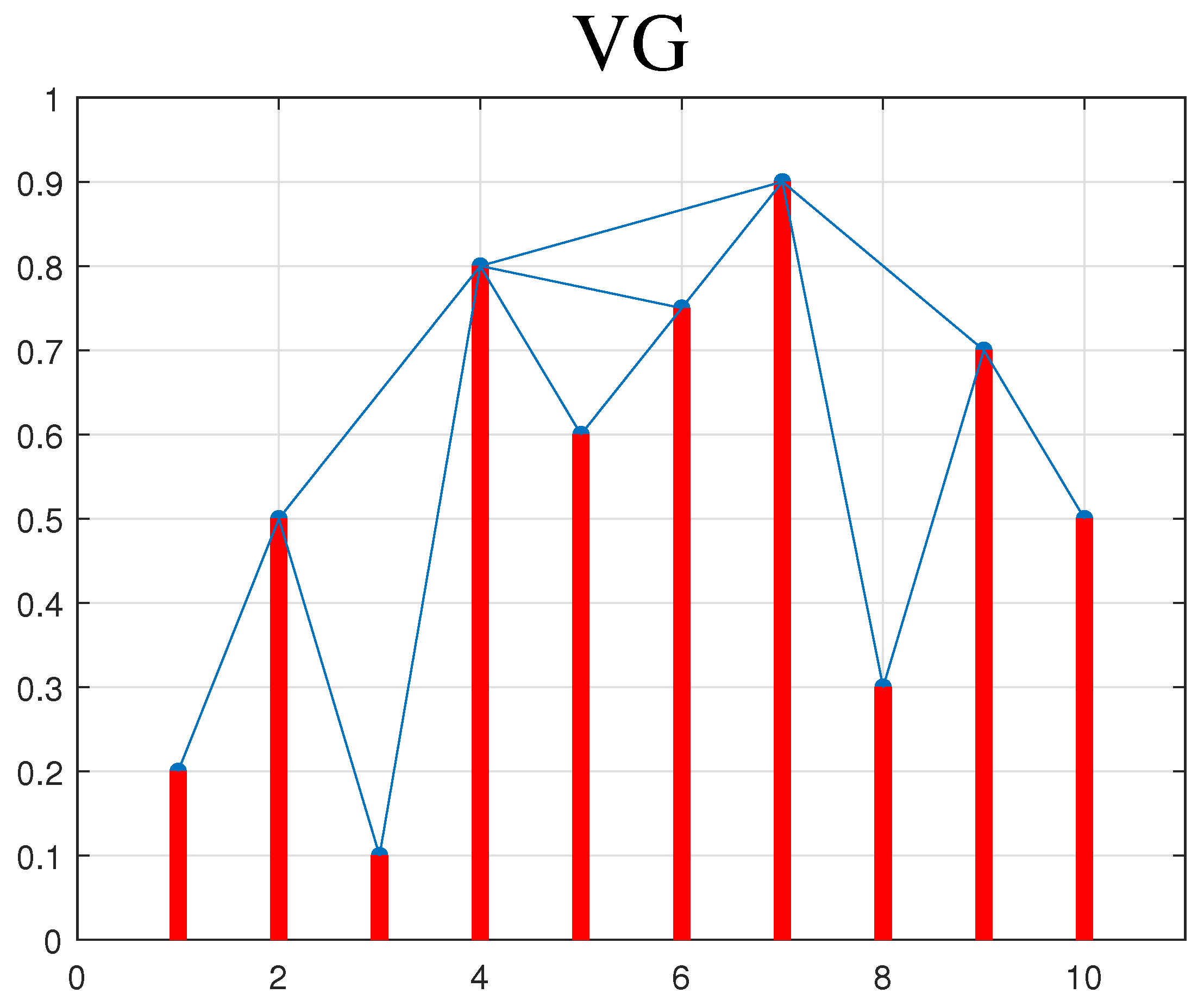
Figure 1. Schematic of the visibility graph algorithm.
Applsci 15 03015 g001
Figure 2. Schematic of the horizontal visibility graph algorithm.
Applsci 15 03015 g002
Figure 3. LPVG with the limited penetrable distance L is set to L = 1.
Applsci 15 03015 g003
Figure 4. Example of the QG method for a time series with T = 12 , Q = 4 , k = 1 .
Applsci 15 03015 g004
Figure 5. Example of MFDM for time series with Q = 4 in divisible case.
Applsci 15 03015 g005
Figure 6. Example of MFDM for time series with Q = 4 in non-divisible case. The different color represents two stages of related algorithm, i.e., stage 1: connecting the node to its neighbours (lines in green); stage 2: connecting nodes in same divided aera (lines in blue).
Applsci 15 03015 g006
Figure 7. Comprehensive framework flowchart of our algorithms.
Applsci 15 03015 g007
Figure 8. Typical EEG signals in each of the five sets; from top to bottom: (A) (healthy, eyes open), (B) (healthy, eyes closed), (C) (epileptic, opposite zone), (D) (epileptic, epileptogenic zone), and (E) (epileptic, seizure).
Applsci 15 03015 g008
Figure 9. Box plot of Δ obtained using the Q G method for groups A, B, C, D, and E, with Q = 30 and k = 4 .
Applsci 15 03015 g009
Figure 10. Confusion matrix diagram of the XGBoost model under a binary classification task.
Applsci 15 03015 g010
Figure 11. The ROC curve of the XGBoost model in the binary classification task.
Applsci 15 03015 g011
Figure 12. Accuracy % of the top ten models for binary classification tasks.
Applsci 15 03015 g012
Figure 13. Accuracy of the CNN method for binary classification task.
Applsci 15 03015 g013
Figure 14. Confusion matrix diagram of CNN method under binary classification task.
Applsci 15 03015 g014
Figure 15. The confusion matrix diagram of the XGBoost model under a five-class classification task.
Applsci 15 03015 g015
Figure 16. The ROC curve of the XGBoost model in the five-class classification task.
Applsci 15 03015 g016
Figure 17. Accuracy % of the top ten models for five classification tasks.
Applsci 15 03015 g017
Figure 18. Accuracy of the CNN model in the five-class classification task.
Applsci 15 03015 g018
Figure 19. Confusion matrix diagram of CNN model in the five-class classification task.
Applsci 15 03015 g019
Table 1. The p-value of the computed features in our numerical experiments.
Featurep-Value
ρ V G 5.47167 × 10 38
D V G 5.44559 × 10 1
M V G 3.59848 × 10 24
α V G 5.47167 × 10 38
C V G 6.75227 × 10 77
L V G 2.50911 × 10 2
G V G 1.13543 × 10 18
ρ H V G 1.59894 × 10 93
D H V G 9.96596 × 10 65
M H V G 1.25973 × 10 32
α H V G 1.59894 × 10 93
C H V G 3.52079 × 10 71
L H V G 1.73161 × 10 82
G H V G 8.53595 × 10 99
ρ L P V G 1.51657 × 10 46
D L P V G 8.10539 × 10 1
M L P V G 6.97230 × 10 24
α L P V G 1.51657 × 10 46
C L P V G 4.33977 × 10 94
L L P V G 1.77361 × 10 3
G L P V G 1.87006 × 10 14
ρ M F D M 4.01871 × 10 12
D M F D M 9.98876 × 10 10
M M F D M 5.32264 × 10 8
α M F D M 4.01871 × 10 12
C M F D M 3.14236 × 10 8
L M F D M 4.56050 × 10 8
G M F D M 1.13674 × 10 10
Δ Q G 1.55180 × 10 130
Table 2. Model evaluation indicators in binary classification task.
MethodAccuracyBalanced AccuracyF1 ScorePrecisionRecallSpecificityMCCCohen’s KappaHamming LossJaccard Index
VG0.8820.8790.9010.9080.8930.8650.7550.7550.1180.820
HVG0.9340.9310.9450.9440.9470.9150.8620.8620.0660.896
LPVG0.9280.9280.9390.9520.9270.9300.8510.8510.0720.885
MFDM0.8400.8330.8670.8640.8700.7950.6660.6660.1600.765
QG0.7960.7840.8320.8210.8430.7250.5720.5720.2040.713
Ours0.9780.9780.9820.9830.980.9750.9540.9540.0200.964
Table 3. Results of different classifiers on binary classification tasks.
RankModel TypeAccuracy (%)Total CostPresetPrediction Speed (obs/s)Training Time (s)
1Ensemble97.612Custom Ensemble274.21168.61
2SVM97.413Custom SVM20,898.5541.13
3Ensemble97.413Bagged Trees2703.393.53
4Neural Network97.214Custom Neural Network17,686.34165.26
5Tree97.214Custom Tree13,993.0217.42
6SVM97.214Cubic SVM14,767.651.11
7Kernel97.214SVM Kernel17,235.551.84
8Neural Network97.015Trilayered Neural Network17,110.861.03
9Tree96.816Fine Tree22,969.391.72
10Tree96.816Medium Tree21,404.113.76
11SVM96.816Medium Gaussian SVM12,757.802.04
12Ensemble96.816RUSBoosted Trees6180.082.12
13Ensemble96.617Subspace KNN924.603.72
14Neural Network96.617Medium Neural Network21,523.244.87
15SVM96.418Quadratic SVM15,984.761.40
16KNN96.219Custom KNN4506.5018.77
17KNN96.219Fine KNN7484.533.06
18Neural Network96.219Narrow Neural Network16,441.531.68
19Neural Network96.219Wide Neural Network22,565.421.03
20Neural Network96.219Bilayered Neural Network20,544.011.62
21KNN96.020Weighted KNN8537.682.07
22Kernel96.020Logistic Regression Kernel16,205.771.09
23Tree95.821Coarse Tree16,004.922.09
24SVM95.821Linear SVM12,219.592.11
25Logistic Regression95.423Logistic Regression4623.443.51
26KNN95.224Medium KNN7554.551.69
27Naive Bayes94.826Custom Naive Bayes2382.3163.52
28Naive Bayes94.826Kernel Naive Bayes1967.083.54
29KNN94.826Cosine KNN7863.220.83
30SVM94.627Fine Gaussian SVM12,950.650.79
31KNN94.627Cubic KNN5804.980.95
32Discriminant92.438Custom Optimizable Discriminant9477.0728.42
33Naive Bayes92.438Gaussian Naive Bayes4518.483.67
34SVM91.244Coarse Gaussian SVM14,743.481.92
35Ensemble90.647Subspace Discriminant1371.423.28
36Discriminant89.453Linear Discriminant12,721.641.16
37KNN86.667Coarse KNN7719.472.57
38Ensemble60.0200Boosted Trees19,922.382.83
Table 4. Model evaluation indicators in the five-class classification task.
MethodAccuracyBalanced AccuracyF1 ScorePrecisionRecallSpecificityMCCCohen’s KappaHamming LossJaccard Index
VG0.5680.5680.5710.5760.5680.8920.4600.4600.4320.406
HVG0.7280.7280.7280.7290.7280.9320.6600.6600.2720.592
LPVG0.5940.5940.5960.6030.5940.8990.4930.4930.4060.430
MFDM0.4700.4700.4690.4690.4700.8680.3380.3380.5300.309
QG0.4380.4380.4360.4350.4380.8600.2980.2980.5620.291
Ours0.8240.8240.8230.8230.8240.9560.7800.7800.1760.715
Table 5. Results of different classifiers in five classification tasks.
RankModel TypeAccuracy (%)Total CostPresetPrediction Speed (obs/s)Training Time (s)
1SVM82.090Custom SVM10,505.95249.81
2SVM81.294Linear SVM3907.474.57
3Ensemble81.095Custom Ensemble3021.8788.07
4SVM80.896Quadratic SVM3794.014.37
5Neural Network80.697Custom Neural Network21,322.14261.35
6Neural Network80.697Medium Neural Network10,889.954.83
7Neural Network80.0100Wide Neural Network22,057.922.10
8Ensemble79.2104Bagged Trees2281.525.26
9SVM79.0105Cubic SVM3244.704.26
10SVM78.6107Medium Gaussian SVM2875.674.03
11Ensemble78.2109Boosted Trees2966.543.95
12Tree77.8111Fine Tree5292.958.34
13Tree77.8111Custom Tree8286.8425.31
14Neural Network77.8111Narrow Neural Network13,850.455.43
15Neural Network77.6112Trilayered Neural Network14,166.037.04
16Neural Network77.4113Bilayered Neural Network13,540.195.83
17KNN76.8116Custom KNN6235.3726.83
18Kernel76.4118Custom Kernel5609.9410.26
19Ensemble74.8126Subspace Discriminant1279.074.06
20KNN74.6127Weighted KNN4769.252.09
21Kernel74.6127Custom Kernel5119.615.70
22Tree74.4128Medium Tree11,200.870.97
23Ensemble74.2129RUSBoosted Trees2949.143.89
24Ensemble73.8131Subspace KNN893.565.70
25Discriminant72.2139Optimizable Discriminant7123.5130.54
26Discriminant72.2139Linear Discriminant11,343.243.04
27Naive Bayes71.6142Custom Naive Bayes967.91111.53
28Naive Bayes71.6142Custom Naive Bayes822.897.32
29KNN71.6142Fine KNN5459.713.28
30KNN71.0145Cosine KNN4489.382.32
31SVM70.4148Coarse Gaussian SVM5785.775.28
32KNN70.0150Medium KNN4529.331.64
33KNN69.0155Cubic KNN3553.802.20
34Naive Bayes67.0165Gaussian Naive Bayes2288.752.76
35SVM67.0165Fine Gaussian SVM2990.764.15
36Tree65.2174Coarse Tree11,090.563.89
37KNN58.6207Coarse KNN4593.061.23
Disclaimer/Publisher’s Note: The statements, opinions and data contained in all publications are solely those of the individual author(s) and contributor(s) and not of MDPI and/or the editor(s). MDPI and/or the editor(s) disclaim responsibility for any injury to people or property resulting from any ideas, methods, instructions or products referred to in the content.