Article

Analysis of the Hourglass–Spindle-Shaped Trajectory Generated by the Collision of Circularly Polarized Laser Pulses with Electrons

1
Bell Honors School, Nanjing University of Posts and Telecommunications, Nanjing 210023, China
2
College of Science, Nanjing University of Posts and Telecommunications, Nanjing 210023, China
3
School of Communications and Information Engineering, Nanjing University of Posts and Telecommunications, Nanjing 210023, China
*
Author to whom correspondence should be addressed.
Appl. Sci. 2025, 15(6), 3013; https://doi.org/10.3390/app15063013
Submission received: 24 January 2025 / Revised: 7 March 2025 / Accepted: 9 March 2025 / Published: 11 March 2025

Abstract

:
This study investigates the hourglass–spindle-shaped trajectory of electron motion based on a model of electron and circularly polarized chirped laser pulse coaxial collision. The velocity, acceleration, and radiation distribution of the electron in this state of motion are systematically analyzed. The formation process of the hourglass–spindle-shaped trajectory is examined in detail. Four distinct stages of the electron–laser pulse collision process are proposed, with an in-depth analysis of the interaction dynamics and underlying mechanisms in each stage. The critical conditions for the formation of the hourglass–spindle-shaped trajectory are identified, along with the conditions for the emergence of two other possible trajectories resulting from the collision: the spiral-shaped and spindle-shaped trajectories. Additionally, a general model for analyzing electron–laser pulse collisions is proposed.

1. Introduction

Due to the high directionality and high coherence of laser pulses, precise control can be achieved by adjusting laser parameters during laser–matter interactions. By designing parameters such as the polarization direction, chirp parameter, pulse width, beam waist radius, and repetition rate of the laser pulse, precise control over the interaction between the laser pulse and electrons can be achieved. Furthermore, controlling the initial position, energy, and motion direction of the electrons enables the interaction between the electron and laser pulse in different scenarios. Through simulations of experiments under various conditions, corresponding data for real-world situations can be obtained, thereby providing a reference for actual experiments. Laser–matter interactions have numerous application scenarios, making this field a subject of extensive research by many scholars [1,2,3]. Among these, nonlinear Thomson scattering has become a particularly popular research direction, and the nonlinear Thomson scattering of intense laser pulses in single electrons, particle beams, plasmas, and other materials has significant research value [4,5,6]. Thomson scattering refers to the elastic scattering of electromagnetic radiation by a free charged particle. During the scattering process, the frequency of the photon remains unchanged. When an electron is scattered by electromagnetic radiation, the electric field component causes the electron to undergo forced oscillations. According to classical electromagnetism, the oscillating electron radiates electromagnetic waves in all directions, which results in scattered X-rays, with the radiation primarily distributed in the forward direction of the incident electromagnetic radiation. On the other hand, nonlinear Thomson scattering occurs when electrons are driven by intense fields, causing their motion to become more complex. The equations of motion exhibit nonlinear characteristics under such conditions [7,8,9,10]. In the late 1980s, Maine et al. proposed the technique of Chirped Pulse Amplification (CPA) [11]. The advent of chirped pulses further enhanced the intensity and quasi-stability of laser pulses, enabling the generation of higher-quality pulses [12], and it has given rise to applications in various fields, including laser pulse amplifiers, electron dynamics, and more [13,14,15,16,17,18]. Considering the high costs associated with the instruments, manpower, and material preparation required for conducting nonlinear Thomson scattering experiments, as well as the difficulty in performing large-scale experiments on individual electrons, simulations through computational experiments offer a more efficient approach. Such simulations allow for large-scale data acquisition and analysis in a relatively shorter time and at a lower cost. Therefore, the simulation of nonlinear Thomson scattering and the subsequent data analysis through simulations hold significant research value.
In recent years, with the continuous development of ultrashort and ultra-intense chirped laser pulses, nonlinear Thomson scattering induced by electrons under relativistic laser pulse intensities has attracted significant attention. For example, Wang et al. [19] investigated the spatial radiation characteristics of interactions between circularly polarized laser pulses and electrons. Yousef et al. [20] studied attosecond and zeptosecond X-ray pulses generated by nonlinear Thomson backscattering and found that variations in the laser pulse beam waist affect the pulse shape and monochromaticity of the process.
Building upon the aforementioned studies, this paper analyzes the interaction between circularly polarized chirped pulses and electrons in a coaxial collision process, discovering a novel trajectory—an hourglass–spindle shape. The trajectory is defined and analyzed, and the principles and process of its formation are determined. By adjusting laser pulse parameters, it is possible to reverse the motion of the electrons, which is preliminarily speculated to have significant potential for electron trapping and trajectory control. This could exhibit even greater effects and benefits in future research. This experiment has a high practical application value and provides a theoretical analysis for the special trajectory electrons generated in practical nonlinear Thomson scattering experiments. This paper explains the pulse laser parameters and mechanisms that lead to the generation of special trajectory electrons, offering corresponding theoretical parameters for electron trajectory control. It also presents an innovative analytical model and approach for analyzing the interaction between free electrons and pulse lasers in a coaxial collision scenario. Furthermore, this paper extends the theoretical analysis of the interaction between free electrons with different initial positions and velocity directions and chirped pulse lasers. Other directions, such as off-axis collisions (i.e., non-coaxial), multi-electron systems, and plasma–laser interactions, still hold significant research value, and this study can serve as a reference for these extended areas. By combining the interaction and cross-analysis of single electrons, plasma, and lasers from various angles, initial positions, and velocity directions, the simulation of actual experimental scenarios can be significantly improved in terms of rationality and accuracy. In the future, this can be further developed into a computerized simulation laboratory for electron–laser pulse interactions, achieving standardized and scaled control of simulated experiments and improving the reliability and effectiveness of experiments and data collection.

2. Materials and Methods

The spatial and temporal coordinates in all the physical quantities are normalized by k 0 1 = λ 0 / 2 π and ω 0 1 = λ 0 / 2 π c , where k 0 1 represents the wave number, ω 0 1 represents the laser pulse frequency, λ 0 = 1   μ m is the laser pulse wavelength, and c = 2.998 × 10 8   m / s is the speed of light. In this study, the observer is used as the reference frame, with t defined as the time in the observer’s frame. For ease of analysis, we introduce the electron’s reference frame and define t e = t R + n j as the time in the electron’s reference frame for the derivation, where R is the distance between the observer and the interaction center, and j = ( x t e , y t e , z t e ) is the electron’s displacement at time t e . The radiation direction is n = ( sin θ cos ϕ , sin θ sin ϕ , cos θ ) , where θ is the polar angle, and ϕ is the azimuthal angle. The initial position of the electron, ( x 0 , y 0 , z 0 ) , is set as ( 0 , 0 , 0 ) , where the electron moves along the negative z -axis from the origin and undergoes a coaxial collision with the laser pulse propagating along the positive z -axis.
The interaction process between chirped pulses and electrons is illustrated in Figure 1. In a tightly focused Gaussian laser pulse field, the motion of electrons can be described by the electric field E and magnetic field B , which satisfy Maxwell’s equations [21]:
E = × A
B = ϵ   [ ( i / k ) ( · A ) + i k A ]
where ϵ is the permittivity, the solution A to the Helmholtz equation is as follows:
2 A + k 0 2 A = 0
In the Cartesian coordinate system, circularly polarized laser pulse is synthesized using a pair of linearly polarized lasers with a phase difference of π / 2 , whose polarization planes are perpendicular to the y-axis and x-axis, respectively. Thus, the electromagnetic field of the circularly polarized laser pulse can be decomposed as E = E x p + E y p and B = B x p + B y p . In this model, the Gaussian laser field has a spot size of 2 w 0 , a pulse width of L , and an intensity of I . Therefore, we can define the following:
E 0 = a 0 b 0 b exp η 2 L 2 exp ρ 2 b 2
Here, a 0 = I λ 0 2 / 1.384 × 10 9 represents the peak amplitude, and b = b 0 1 + z 2 / z 0 2 is the beam waist radius, where the Rayleigh range is z 0 = k 0 b 0 2 / 2 . The longitudinal distance is η = z t , and the transverse distance is ρ = x 2 + y 2 . Under tightly focused laser conditions [22], the expressions for the electromagnetic fields must be expanded to higher orders that remain accurate with the diffraction angle ε = b 0 / z 0 . Yousef et al. [2] derived the components A, B, and E in the x-axis linearly polarized laser field from Equations (1)–(3). Zhang [23] and Barton [22] proposed the electromagnetic field expressions for y-axis linearly polarized laser fields using symmetric formulations. Through vector synthesis, the fifth-order expansion of the electric field components E = { E x , E y , E z } can be obtained:
E x = E 0 { S 0 + ε 2 [ α 2 S 2 r 4 S 3 4 ] + ε 4 S 2 8 r 2 S 3 4 r 2 r 2 16 α 2 S 4 16 r 4 r 2 + 2 α 2 S 5 8 + r 8 S 6 32   + ε 2 C 2 + ε 4 [ r 2 C 4 r 4 C 5 4 ] }
E y = E 0 { C 0 + ε 2 [ β 2 C 2 r 4 C 3 4 ] + ε 4 C 2 8 r 2 C 3 4 r 2 r 2 16 β 2 C 4 16 r 4 r 2 + 2 β 2 C 5 8 + r 8 C 6 32 + ε 2 S 2 + ε 4 [ r 2 S 4 r 4 S 5 4 ] }
E z = E 0 α { ε C 1 + ε 3 [ C 2 2 + r 2 C 3 r 4 C 4 4 ] + ε 5 [ 3 C 3 8 3 r 2 C 4 8 + 17 r 4 C 5 16 3 r 6 C 5 16 3 r 6 C 6 8 + r 8 C 7 32 ] } E 0 β { ε S 1 + ε 3 [ S 2 2 + r 2 S 3 r 4 S 4 4 ] + ε 5 [ 3 S 3 8 3 r 2 S 4 8 + 17 r 4 S 5 16 3 r 6 S 5 16 3 r 6 S 6 8 + r 8 S 7 32 ] }
The components of the magnetic field are described as follows:
B x = E 0 { C 0 + ε 2 [ r 2 C 2 2 r 4 C 3 4 ] + ε 4 [ C 2 8 + r 2 C 3 4 + 5 r 4 C 4 16 r 6 C 5 4 + r 8 C 6 32 ] }
B y = E 0 { S 0 + ε 2 [ r 2 S 2 2 r 4 S 3 4 ] + ε 4 [ S 2 8 + r 2 S 3 4 + 5 r 4 S 4 16 r 6 S 5 4 + r 8 S 6 32 ] }  
B z = E 0 β { ε C 1 + ε 3 [ C 2 2 + r 2 C 3 2 r 4 C 4 4 ] + ε 5 [ 3 C 3 8 + 3 r 2 C 4 8 + 3 r 4 C 5 16 r 6 C 6 4 + r 8 C 7 32 ] }   E 0 α { ε S 1 + ε 3 [ S 2 2 + r 2 S 3 2 r 4 S 4 4 ] + ε 5 [ 3 S 3 8 + 3 r 2 S 4 8 + 3 r 4 S 5 16 r 6 S 6 4 + r 8 S 7 32 ] }
where α = x / b 0 , β = y / b 0 , and r = ρ / b 0 . The functions S m and C m are shown as follows:
S m = b 0 b m sin ψ + m ψ G
C m = b 0 b m cos ψ + m ψ G
m = 0 , 1 , 2 ,
The phase is given by ψ = ψ 0 + η ψ R + ψ G + c 0 η 2 , where c 0 η 2 represents the phase shift caused by the chirp, and the initial phase ψ 0 is the phase of the plane wave. ψ R = ρ 2 / 2 R z is the phase related to the wavefront curvature, where R z = z + z 0 2 / z is the radius of curvature of the wavefront at the z-coordinate where it intersects the beam axis. ψ G = tan 1 z / z 0 is the additional phase change experienced by the Gaussian beam, indicating that as the beam travels from to + , it undergoes a total phase change.
It is important to note that, regarding the expansion of the formula to exactly the fifth order, our explanation is as follows: Although most theoretical studies of electron laser acceleration use low-order Gaussian or Bessel beams, our goal is to achieve electron radiation at GeV or even TeV energy levels, which requires extremely high-intensity laser fields. In Yousef et al.’s study [2], it was pointed out that using low-order Gaussian or Bessel beams to describe such high-intensity laser fields leads to inaccuracies. They pointed out that for tightly focused beams with a waist radius ω 0 (denoted as b 0 in this paper) smaller than 4 μm, the fifth-order correction terms satisfy both the accuracy and computational complexity requirements: For ultra-strong lasers, corrections beyond the fifth order are required to ensure accuracy in the description, and the fifth-order correction is sufficient for describing this situation, even for smaller ω 0 values. Therefore, further increasing the correction order may lead to redundant computational effort. Thus, our design conditions and the derivation of the formula use a fifth-order field description to more accurately describe tightly focused laser pulses while avoiding excessive computational overflow.
Considering the rest mass of a single electron m e = 9.1096 × 10 31   kg and its charge e = 1.6022 × 10 19   C , we determine and describe the electron’s motion in a strong laser pulse using the following Lorentz equation and energy equation:
d p d t e = e E + u × B
d Γ d t e e c u · E
where Γ = γ 0 m e c 2 represents the electron’s energy, defined by the formula γ 0 1 = 1 u 2 , where γ 0 is the Lorentz factor, representing the electron’s normalized initial energy. The electron’s momentum is p = Γ v / c 2 , where v is the electron’s velocity and u = v / c . It is assumed that the direction of the electron’s velocity is opposite to the direction of laser propagation.
The time-varying electromagnetic field produced by a moving charged particle can be derived from the Lienard–Wiechert potential [24]. Therefore, the radiation power per unit solid angle can be calculated as follows:
d P t e d Ω = n × n u × d t u 2 ( 1 n u ) 6 t
The radiation pulse power d P ( t e ) / d Ω is normalized to e 2 b 0 2 / 4 π c . The different time subscripts in Equation (15) indicate that the pulse received by the observer at time t is actually emitted by the electron at time t e .
The data were obtained by solving the ordinary differential Equations (13) and (14) using the 4–5 Runge–Kutta–Fehlberg method (RKF45). A large-scale GPU parallel computation is performed on MATLAB R2023a, recording the numerical solutions for the electron’s position, velocity, and acceleration at each step. The radiation at different spacetime states can be derived from Equation (15), and relevant plots of the electron’s characteristics are obtained through data visualization.

3. Results

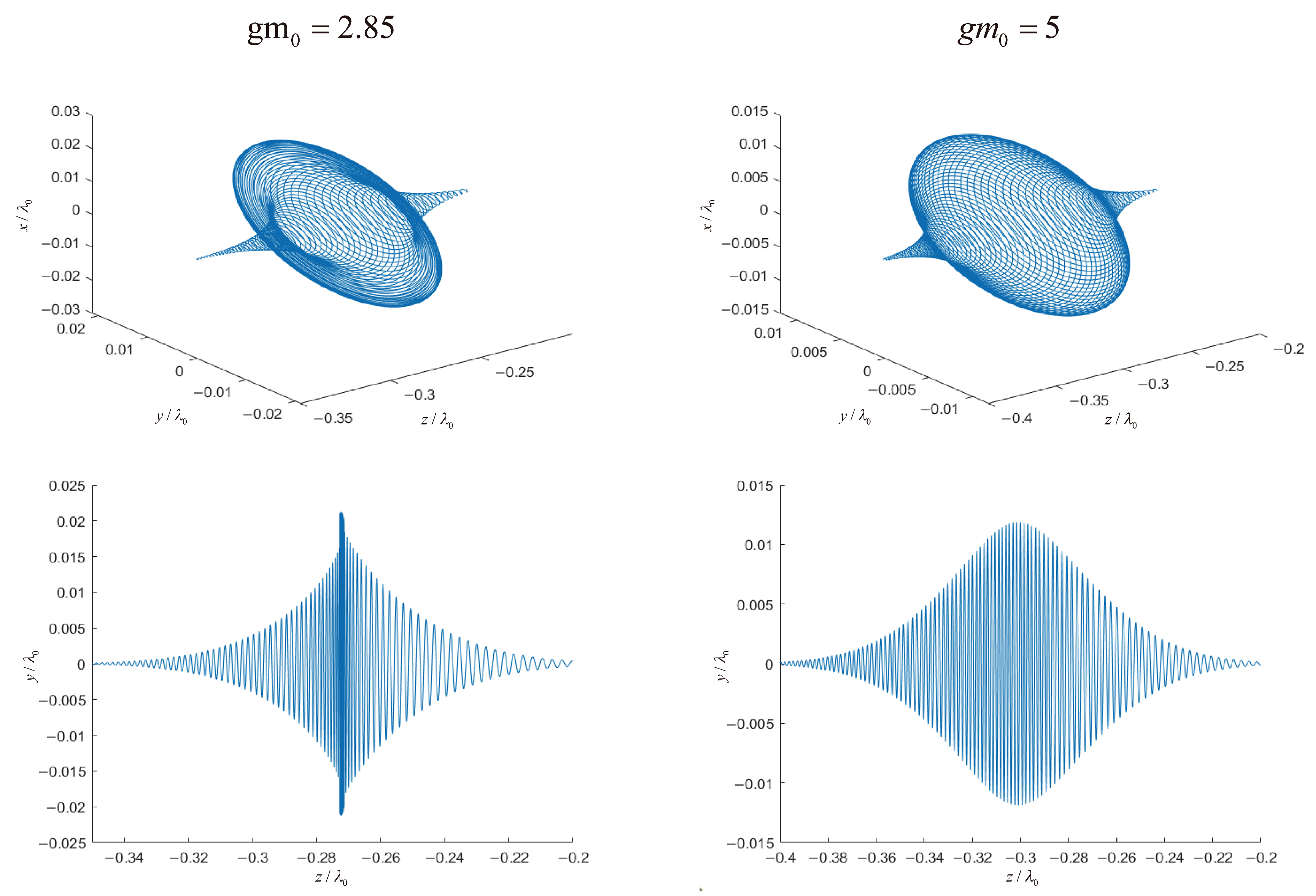
3.1. Motion Trajectory Analysis

The initial position of the electron is at the origin of the coordinate system. The incident circularly polarized laser chirped pulse is an electromagnetic wave, with the transverse electric field and irradiance distribution approximately following a Gaussian envelope, propagating in the +z direction with an incident angle of 0°. The wavelength λ 0 = 1   μ m , the intensity parameter a 0 = 5 (corresponding to I = 3.45 × 10 19   W / c m 2 ), and the chirped pulse width L is 3 λ 0 . The beam waist radius b 0 is determined to be 4 λ 0 , and the chirp parameter c 0 is set to 0.03 . The laser propagates in the positive z-axis direction, while the electron’s velocity is directed along the negative z-axis. The normalized initial energy of the electron is Γ 0 = 2 . T s p a n represents the duration of the interaction process, which corresponds to the time used to solve the partial differential equations, and it also indicates the measurement period of the model.
By analyzing the electron’s motion at different t s p a n , the parameters of the electron interacting with the laser pulse up to a specific state can be obtained. The electron undergoes head-on collision with the laser pulse along the z-axis, and the influence of the laser pulse causes the electron to exhibit the motion trajectory shown in Figure 2. We define the motion along the z-axis as axial motion characteristics, while the motion in the x o y plane is described as radial motion characteristics. Notably, after interacting with the laser pulse, the electron’s trajectory envelope forms an inner shape resembling an hourglass and an outer shape resembling an elliptical spindle, which is defined as the “hourglass-spindle shape”. This paper focuses on analyzing the formation process of the hourglass–spindle-shaped trajectory and the variation of its related parameters.

3.1.1. The Coupling Analysis of Motion Trajectory and Radiation Power

To facilitate the analysis of the relationship between the electron’s position at a specific moment and its corresponding radiation, the z-axis is transformed into η = z t , representing the entire interaction process between the electron and the laser pulse. The radiation values during the interaction process are mapped to the electron’s trajectory using color coding. From the color bar of the radiation curve and the motion trajectory, the energy distribution of the electron in different states can be observed. It is important to note that, due to the significant variation in radiation values released throughout the electron’s motion, the radiation values and color bar distribution in each figure are normalized to the maximum radiation value released up to that point in time. After the complete evolution process, the formation of the hourglass–spindle-shaped trajectory can be divided into four stages. The motion trajectories and radiation power distributions for these four stages are shown in Figure 3.
The axial and radial acceleration, as well as the velocity changes during the motion process, are calculated separately. The magnitude and direction of the axial and radial acceleration are plotted as a function of η in Figure 4. The orange vertical lines or orange dots marked in Figure 4 indicate the positions where the electron exactly reaches the central axis of the laser pulse. These markers are used to distinguish between the rising edge and the falling edge interaction regions. Hereafter, this position is referred to as the central position of the laser. By combining Figure 3 and Figure 4, we can conduct a more accurate analysis of the electron’s motion at different stages. During the forward collision between the electron and the laser pulse, the electron undergoes two reversals in its axial motion direction along the z-axis. The axial acceleration exerted by the laser pulse on the electron initially increases in the negative z-axis direction, then decreases to 0, and subsequently transitions to the positive z-axis direction, where it again increases and then decreases to 0, marking the end of its effect on the electron. By conducting a time-evolution analysis of the velocity and acceleration, the reasons for the axial reversals in the electron’s trajectory are further explained here:
Under the influence of a strong laser field, the relativistic motion of electrons is affected by the electric field and the ponderomotive potential. The electric field primarily causes high-frequency oscillations of the electron in the radial direction (within the x-y plane), while the ponderomotive potential dominates the electron’s axial motion (along the z-axis). The ponderomotive potential can be regarded as the gradient of the normalized Lorentz factor, reflecting changes in the electron’s velocity and energy. Gaussian laser pulses follow a Rayleigh distribution in the radial direction, with the beam waist radius first increasing and then decreasing along the axial direction.
At z = 0 , the beam waist radius reaches its maximum, where the laser pulse’s focusing effect is strongest, meaning the laser pulse’s influence on the electron trajectory is most significant. The electric field generated by the laser pulse causes the electron’s radial motion radius to first expand and then contract. The main reason for the change in the electron’s radial motion radius is the Rayleigh distribution of the laser pulse, where the radial component of the laser pulse’s acceleration on the electron resembles the laser pulse distribution. This causes the electron to undergo radial oscillations under the influence of the electric field. In the axial direction, the laser pulse’s axial component exerts alternating acceleration and deceleration on the electron, causing velocity changes due to the influence of the ponderomotive force. Based on this condition, the axial motion process of the electron is further analyzed:
Phase 1: During this stage ( t s p a n = 0 ~ 58 ), the electron, with an initial velocity, comes into contact with the rising edge of the laser pulse. According to Phase 1, shown in Figure 3, the electron’s velocity direction is along the negative z-axis, while the axial component of the ponderomotive potential of the laser’s rising edge points in the positive z-axis direction. From the color bar of the radiation distribution, we can see that in Phase 1, the electron’s radiation power increases as the interaction process progresses. In Figure 4, the acceleration in the z-axis increases negatively in Phase 1. The axial component of the ponderomotive potential acts to decelerate the electron, reducing its axial velocity.
Phase 2: According to Figure 4, during this stage ( t s p a n = 58 ~ 74 ), under the condition g m 0 = 2 , the electron’s axial velocity reaches a point where it decreases to 0. However, at this moment, the electron does not cross the central axis of the laser pulse and continues to interact with the rising edge of the laser pulse. Therefore, the axial component of the ponderomotive potential remains in the positive z-axis direction, and the electron starts to accelerate in the positive z-axis direction due to this effect. In addition, from the electron’s motion trajectory and radiation power distribution in Figure 3, we can see that the radiation power of the electron in this stage is still monotonically increasing, with no decrease observed. This is consistent with the above conclusion, and at this point, the effect of the laser on the electron is similar to that in Phase 1.
Phase 3: In the third stage, as the electron passes the central position, the acceleration curve begins to decrease, which can be seen in Figure 4. During this stage ( t s p a n = 74 ~ 96 ), the electron undergoes reverse acceleration, but its velocity remains lower than the speed of the laser pulse. As a result, the laser pulse continues to move relative to the electron along the positive z-axis, effectively passing through the electron. At this point, the central axis of the laser pulse surpasses the electron, causing the electron to interact with the falling edge of the laser pulse. The axial component of the ponderomotive potential of the laser pulse’s falling edge reverses to the negative z-axis direction. However, due to the influence of the second phase, the electron’s axial velocity component remains in the positive z-axis direction. Consequently, the electron begins to decelerate for the second time under the influence of the laser pulse. In Figure 3 of Phase 3, based on the mapping relationship between radiation and motion trajectory, it can be observed that the radiation power of the electron begins to decline. The peak radiation power appears at the transition between Phase 2 and Phase 3, which occurs when the central position of the laser interacts with the electron. At this moment, the electron experiences the maximum influence of the electric field, resulting in the highest radiation power.
Phase 4: In Phase 4 of Figure 3, we can see that the electron’s radiation power does not increase. After the electron returns to the same state as its initial motion direction, the radiation gradually decreases, with a peak present. Based on Phase 4 of Figure 3, we observe that the peak of the radiation power occurs at the position where the electron’s velocity reverses, meaning the radiation peak appears in Phase 3. During this stage ( t s p a n from 96 to the end of the interaction between the electron and the laser pulse), the electron’s velocity decreases to 0 once again. At this point, the electron and the laser pulse have not yet separated, and the electron continues to interact with the falling edge of the laser pulse, undergoing a second phase of reverse acceleration. After the electron and the laser pulse separate, the electron no longer experiences the laser pulse’s influence and proceeds in linear motion.
Through the analysis of this model, the general interaction process between the electron and the laser pulse can be summarized. The electron is influenced by the ponderomotive potential, which is directly proportional to the laser pulse amplitude and inversely proportional to the initial energy of the electron. The greater the initial energy of the electron, the less it is affected by the ponderomotive potential, and the less likely its motion state is to change. Conversely, the greater the laser pulse amplitude and the higher the laser pulse intensity, the stronger the confinement force exerted on the electron, resulting in a greater impact on the electron’s motion. The direction of the force is influenced by the relative position of the electron and the laser pulse, and it always manifests as a repulsive effect on the electron, with the force directed from the laser pulse toward the electron being acted upon.
The radial motion of the electron is influenced by the Rayleigh distribution of the laser pulse, exhibiting a Gaussian distribution in both the x and y directions. Since the interaction between the electron and the laser pulse does not occur at the coordinate origin, the radial motion is affected by the beam waist and chirp of the laser pulse. Consequently, the envelope of the acceleration experienced by the electron in the x and y directions exhibits an asymmetric double-peak distribution.

3.1.2. Further Conclusion

According to the conclusions above, we can further deduce that if the electron’s initial energy is increased or the laser pulse amplitude is reduced, there should be a critical condition where the electron’s velocity at the end of the first phase just decreases to 0. That is, when the radial velocity of the electron decreases to 0, it will just cross the central axis of the laser pulse. After crossing the central axis, the electron begins to interact with the falling edge of the laser pulse, and the electron experiences the negative z-axis ponderomotive force, causing its velocity to increase from 0 in the original direction, thus directly transitioning from the first phase to the fourth phase. If the initial energy exceeds this critical value, the velocity will behave similarly, transitioning directly from the first phase to the fourth phase, but the electron’s velocity will not drop to 0.
Through testing, it was found that when the normalized initial energy of the electron is increased to g m 0 = 2.85 , the electron does not undergo reversal. Its axial velocity reaches 0, while the radial radius continues to change under the influence of the pulse, resulting in a trajectory envelope with a radial ring-shaped protrusion in the middle, resembling a gong shape. As the electron’s initial energy continues to increase, the deceleration of radial motion becomes less noticeable, and the trajectory exhibits the typical spindle shape. For example, at g m 0 = 5 , the trajectory appears as shown in Figure 5. Therefore, the above analysis and conclusions are verified to be correct.

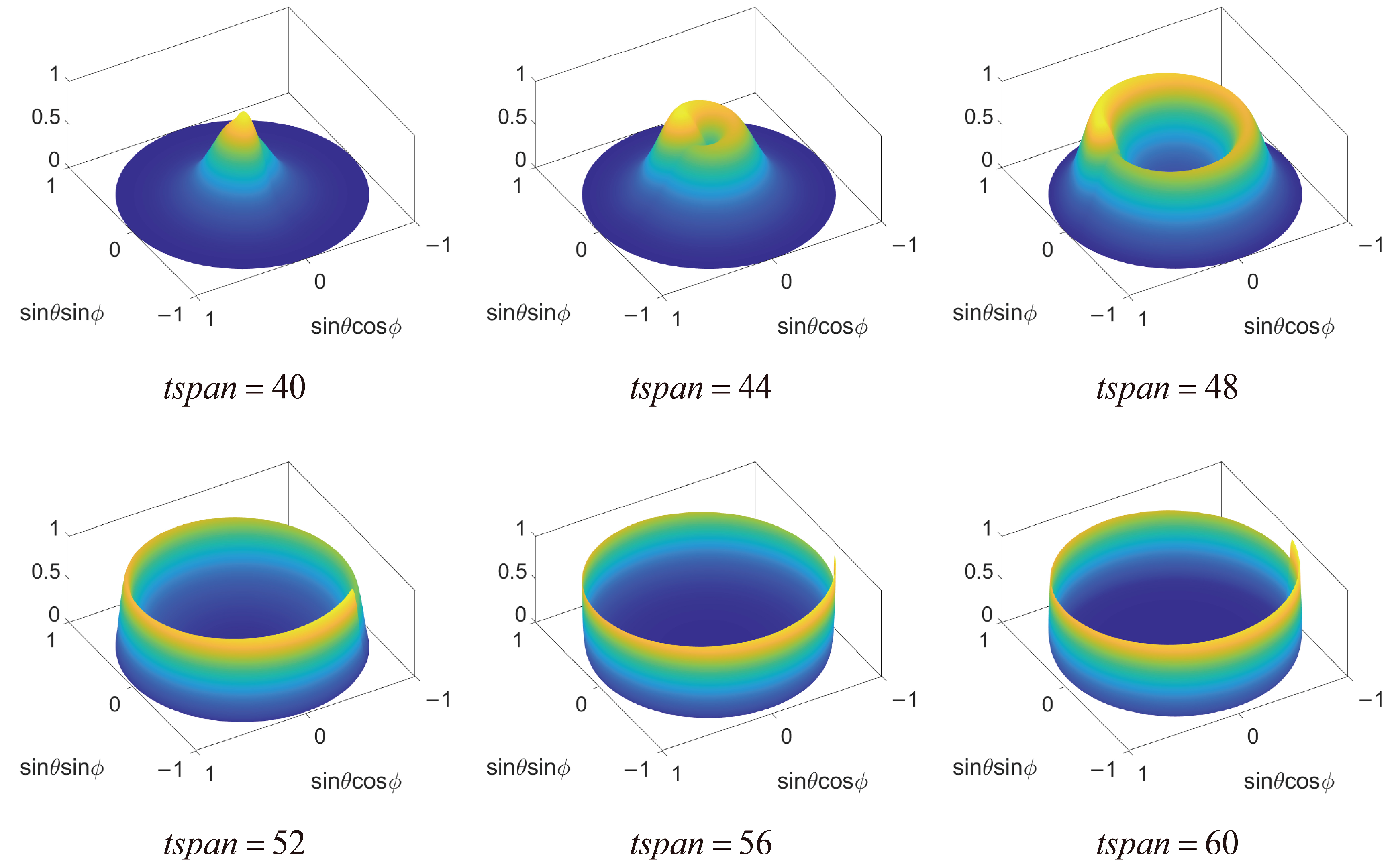
3.2. Radiation Spatial Distribution Variation

It is worth noting that during the interaction with the laser pulse, the electron also exhibits changes in the shape of its radiation spatial distribution. The shape of the radiation distribution transitions from a central peak to a vortex and then to a ring, which is similar to normal models. Notably, the change in the radiation shape occurs between approximately t s p a n = 40   a n d   60 , while the electron’s motion states change at t s p a n = 58 ,   74 ,   and   96 . Therefore, the shape change of the radiation spatial distribution only occurs in the first phase. At the same time, during the fourth stage, as the interaction between the electron and the laser pulse diminishes, a reverse change in the radiation spatial distribution shape similar to that in the first stage will also occur. In the second and third phases, the radiation spatial distribution remains ring-shaped, with only the radiation peak gradually increasing. This indicates that the two reversals in the electron’s motion during the process affect the radiation shape, but the change in motion direction only alters the primary radiation direction without affecting the shape of the radiation distribution.
Figure 6 shows the changes in the radiation spatial distribution shape during the electron’s motion process, with t s p a n taken from 40 to 60. Since we are only focused on the change in the radiation shape during the interaction process, the maximum value of the radiation is normalized for easier observation of the change in the electron’s radiation shape. From the figure, it can be seen that during the first phase of the electron’s motion, the radiation shape changes from a peak to a vortex and then to a ring. This is due to the increasing amplitude of the laser pulse and the decreasing beam waist radius over time, which enhances the laser pulse’s confinement effect on the electron, making the radiation distribution more compact. The thickness of the high-radiation ring decreases, and the radius of the radiation ring increases as the laser pulse amplitude increases, resulting in changes in the observed shape distribution of the radiation.

3.3. Time and Frequency Spectrum Distribution of Radiation

After analyzing the motion trajectory and radiation power, this paper also examines the spatial distribution of radiation, as well as its temporal and spectral characteristics, to investigate whether the radiation distribution in other dimensions is affected by the motion trajectory during the interaction between the electron and the laser pulse. The radiation power is primarily distributed at ω 0 < 6000 , with the overall radiation power decreasing as the frequency increases. The temporal and spectral distributions of the radiation are shown in Phase 4 of Figure 7, which also represents the time spectrum and frequency spectrum of the entire process.
At the same time, we independently calculate and plot the time–frequency spectra for the four stages and study the detailed analysis of the radiation power. The time spectrum and frequency spectrum of the radiation for the four stages are shown in Figure 7.
In Figure 7, Phase 1 generates very little energy and exists only in the extremely low-frequency range at ω < 1000 . In Phase 2, the energy begins to increase, with the peak power reaching approximately 5000, and higher-frequency radiation starts to appear in the range of ω < 6000 . Phase 3 is the main stage of radiation generation, during which the radiation energy across all frequency bands increases significantly. Under the conditions described in this paper, the peak power can reach approximately 14,000 . The radiation frequency is distributed within ω < 10,000 , but it is still primarily concentrated in the relatively low-frequency region. The temporal and spectral distributions in Phase 4 are similar to those in Phase 3, with an increase in the power components of certain frequencies based on Phase 3, but without significant changes.

3.4. Further Study

During the interaction between the free electron and the laser pulse, we have identified and studied the motion trajectories that may result from coaxial collisions between the electron and the laser pulse. However, in practical experimental operations, it is impossible to only conduct coaxial collisions. Additionally, the initial position, initial energy, motion direction, and other parameters of the electron will be more diverse. The conditions, such as the laser pulse’s chirp parameters, pulse width, beam waist radius, and the presence of external electromagnetic fields in the environment, are also more complex. In the next article, we will study more complex models to enhance the theoretical guidance of our research for practical experiments.

4. Conclusions

This paper analyzes the formation mechanism and process of the hourglass-shaped and spindle-shaped motion trajectories generated by the coaxial collision of electrons and laser pulses. The radial oscillation of electrons is caused by the influence of the electric field, while changes in axial velocity are due to the effect of ponderomotive force. The ponderomotive force consistently exerts a repulsive effect on the electrons. Critical conditions for axial reversal of the electron and laser pulse have been determined, and the conditions under which hourglass–spindle-shaped, gong-shaped, and spindle-shaped trajectories are produced by electron–laser collisions have been summarized. Additionally, a general analysis framework for the electron–laser interaction model has been proposed.

Author Contributions

Conceptualization, J.L.; Methodology, J.L. and Z.W.; Software, J.L., J.X. and Q.Z.; Validation, J.L.; Formal analysis, J.L. and Z.W.; Investigation, J.L., J.X., Z.W. and Q.Z.; Resources, J.L. and Q.Z.; Data curation, J.L.; Writing—original draft, J.L.; Writing—review & editing, J.L. and Y.T.; Visualization, J.L., J.X. and Z.W.; Supervision, J.L. and Y.T.; Project administration, Y.T.; Funding acquisition, Y.T. All authors have read and agreed to the published version of the manuscript.

Funding

This work has been supported by the National Natural Sciences Foundation of China under grants No. 10947170/A05 and No. 11104291, the Natural Science Fund for Colleges and Universities in Jiangsu Province under grant No. 10KJB140006, and the Natural Sciences Foundation of Shanghai under grant No. 11ZR1441300.

Data Availability Statement

The original contributions presented in the study are included in the article material, further inquiries can be directed to the corresponding author.

Conflicts of Interest

The authors declare no conflicts of interest.

References

  1. Sarachik, E.S.; Schappert, G.T. Classical theory of the scattering of intense laser radiation by free electrons. Phys. Rev. D 1970, 1, 2738. [Google Scholar] [CrossRef]
  2. Salamin, Y.I.; Keitel, C.H. Electron acceleration by a tightly focused laser beam. Phys. Rev. Lett. 2002, 88, 095005. [Google Scholar] [CrossRef]
  3. He, Y.; Yakup, B.; Bake, M.A. Linearly Polarized γ Photon Generation from Unpolarized Electron Bunch Interacting with Laser. Appl. Sci. 2025, 15, 481. [Google Scholar] [CrossRef]
  4. Esarey, E.; Ride, S.K.; Sprangle, P. Nonlinear Thomson scattering of intense laser pulses from beams and plasmas. Phys. Rev. E 1993, 48, 3003. [Google Scholar] [CrossRef]
  5. Zhang, Y.; Yang, Q.; Wang, J.; Gong, X.; Tian, Y. Zeptosecond-Yoctosecond Pulses Generated by Nonlinear Inverse Thomson Scattering: Modulation and Spatiotemporal Properties. Appl. Sci. 2024, 14, 7038. [Google Scholar] [CrossRef]
  6. Lee, K.; Cha, Y.H.; Shin, M.S.; Kim, B.H.; Kim, D. Temporal and spatial characterization of harmonics structures of relativistic nonlinear Thomson scattering. Opt. Express 2003, 11, 309–316. [Google Scholar] [CrossRef] [PubMed]
  7. Compton, A.H. A quantum theory of the scattering of X-rays by light elements. Phys. Rev. 1923, 21, 483. [Google Scholar] [CrossRef]
  8. Lau, Y.Y.; He, F.; Umstadter, D.P.; Kowalczyk, R. Nonlinear Thomson scattering: A tutorial. Phys. Plasmas 2003, 10, 2155–2162. [Google Scholar] [CrossRef]
  9. Glenzer, S.H.; Alley, W.E.; Estabrook, K.G.; De Groot, J.S.; Haines, M.G.; Hammer, J.H.; Jadaud, J.-P.; MacGowan, B.J.; Moody, J.D.; Rozmus, W.; et al. Thomson scattering from laser plasmas. Phys. Plasmas 1999, 6, 2117–2128. [Google Scholar] [CrossRef]
  10. Herold, H. Compton and Thomson scattering in strong magnetic fields. Phys. Rev. D 1979, 19, 2868. [Google Scholar] [CrossRef]
  11. Maine, P.; Strickland, D.; Bado, P.; Pessot, M.; Mourou, G. Generation of ultrahigh peak power pulses by chirped pulse amplification. IEEE J. Quantum Electron. 1988, 24, 398–403. [Google Scholar] [CrossRef]
  12. Ross, I.; Matousek, P.; Towrie, M.; Langley, A.; Collier, J. The prospects for ultrashort pulse duration and ultrahigh intensity using optical parametric chirped pulse amplifiers. Opt. Commun. 1997, 144, 125–133. [Google Scholar] [CrossRef]
  13. Kim, H.Y.; Garg, M.; Mandal, S.; Seiffert, L.; Fennel, T.; Goulielmakis, E. Attosecond field emission. Nature 2023, 613, 662–666. [Google Scholar] [CrossRef] [PubMed]
  14. Calegari, F.; Ayuso, D.; Trabattoni, A.; Belshaw, L.; De Camillis, S.; Anumula, S.; Frassetto, F.; Poletto, L.; Palacios, A.; Decleva, P.; et al. Ultrafast electron dynamics in phenylalanine initiated by attosecond pulses. Science 2014, 346, 336–339. [Google Scholar] [CrossRef]
  15. Zeng, L.; Wang, X.; Liang, Y.; Yi, H.; Zhang, W.; Yang, X. Chirped-Pulse Amplification in an Echo-Enabled Harmonic-Generation Free-Electron Laser. Appl. Sci. 2023, 13, 10292. [Google Scholar] [CrossRef]
  16. Witting, T.; Osolodkov, M.; Schell, F.; Morales, F.; Patchkovskii, S.; Šušnjar, P.; Cavalcante, F.H.M.; Menoni, C.S.; Schulz, C.P.; Furch, F.J.; et al. Generation and characterization of isolated attosecond pulses at 100 kHz repetition rate. Optica 2022, 9, 145–151. [Google Scholar] [CrossRef]
  17. Gaál, P.; Gilinger, T.; Nagyillés, B.; Nagymihály, R.; Seres, I.; Kovács, Á.; Füle, M.; Karnok, M.; Balázs, P.; Novák, T.; et al. A Versatile 100 Hz Laser System with Few-Cycle and TeraWatt Pulses for Applications. Appl. Sci. 2024, 14, 10649. [Google Scholar] [CrossRef]
  18. Paul, P.M.; Toma, E.S.; Breger, P.; Mullot, G.; Augé, F.; Balcou, P.; Muller, H.G.; Agostini, P. Observation of a train of attosecond pulses from high harmonic generation. Science 2001, 292, 1689–1692. [Google Scholar] [CrossRef]
  19. Wang, Y.; Wang, C.; Li, K.; Li, L.; Tian, Y. Spatial radiation features of Thomson scattering from electron in circularly polarized tightly focused laser beams. Laser Phys. Lett. 2020, 18, 015303. [Google Scholar] [CrossRef]
  20. Salamin, Y.I.; Faisal, F.H.M. Harmonic generation by superintense light scattering from relativistic electrons. Phys. Rev. A 1996, 54, 4383. [Google Scholar] [CrossRef]
  21. Yariv, A. Quantum Electronics, 2nd ed.; John Wiley & Sons: New York, NY, USA, 1975; p. 123. [Google Scholar]
  22. Barton, J.P.; Alexander, D.R. Alexander. Fifth-order corrected electromagnetic field components for a fundamental Gaussian beam. J. Appl. Phys. 1989, 66, 2800–2802. [Google Scholar] [CrossRef]
  23. Zhang, S.Y. Accurate correction field of circularly polarized laser and its acceleration effect. J. At. Mol. Sci. 2010, 1, 308–317. [Google Scholar]
  24. Jackson, J.D.; Ronald, F.F. Classical Electrodynamics; Wiley: Hoboken, NJ, USA, 1999; pp. 841–842. [Google Scholar]
Figure 1. The laser pulse and electron coaxial collision model diagram.
Applsci 15 03013 g001
Figure 2. Hourglass−spindle−shaped trajectory.
Applsci 15 03013 g002
Figure 3. Classification of stages in the electron–laser collision process.
Applsci 15 03013 g003
Figure 4. Velocities and accelerations of the electron in different directions.
Applsci 15 03013 g004
Figure 5. Collision trajectories under different initial energies. The upper image is the main view, and the lower image is the front view.
Applsci 15 03013 g005
Figure 6. Changes in the shape of the radiation spatial distribution within the t s p a n = 40 ~ 60 range.
Applsci 15 03013 g006
Figure 7. Time spectrum and frequency spectrum under four phases.
Applsci 15 03013 g007
Disclaimer/Publisher’s Note: The statements, opinions and data contained in all publications are solely those of the individual author(s) and contributor(s) and not of MDPI and/or the editor(s). MDPI and/or the editor(s) disclaim responsibility for any injury to people or property resulting from any ideas, methods, instructions or products referred to in the content.

