Article

Mamba-DQN: Adaptively Tunes Visual SLAM Parameters Based on Historical Observation DQN

by
Xubo Ma
1,2,
Chuhua Huang
1,2,*,
Xin Huang
1,2 and
Wangping Wu
1,2
1
College of Computer Science and Technology, Guizhou University, Huaxi District, Guiyang 550025, China
2
State Key Laboratory of Public Big Data, Guizhou University, Huaxi District, Guiyang 550025, China
*
Author to whom correspondence should be addressed.
Appl. Sci. 2025, 15(6), 2950; https://doi.org/10.3390/app15062950
Submission received: 25 February 2025 / Revised: 6 March 2025 / Accepted: 7 March 2025 / Published: 9 March 2025
(This article belongs to the Special Issue Applications in Computer Vision and Image Processing)

Abstract

:
The parameter configuration of traditional visual SLAM algorithms usually relies on expert experience and extensive experiments, and the parameter configuration needs to be reset as the scene changes, which is a complex and tedious process. To achieve parameter adaptation in visual SLAM, we propose the Mamba-DQN method, which transforms complex parameter adjustment tasks into policy learning assignments for the agent. In this paper, we select the key parameters of visual SLAM to construct the agent action space. The reward function is constructed based on the absolute trajectory error (ATE), and the Mamba history observer is built within the agent to learn the observation trajectory, aiming to improve the quality of the agent’s decisions. Finally, the proposed method was experimented on the EuRoc MAV and TUM-VI datasets. The experimental results show that Mamba-DQN not only enhances the positioning accuracy of visual SLAM and demonstrates good real-time performance but also avoids the tedious parameter adjustment process.

1. Introduction

Visual SLAM (Simultaneous Localization and Mapping) leverages the capture and analysis of image sequences from cameras to estimate the camera position and orientation in unknown environments in real time, while simultaneously constructing 3D maps. It is widely used in fields such as augmented reality (AR), virtual reality (VR), autonomous driving, mobile robots, and drone navigation [1].
The effectiveness of visual SLAM is partially reliant on parameter configurations, such as the number of pyramid layers, nearest neighbor threshold, initial corner point quantity, and keyframe evaluation threshold. These parameters are customarily set through expert experience and extensive experimentation in traditional methods, which is not only time-consuming but also routinely needs to be readjusted in new application scenarios. Thus, academics are engaged in exploring the implementation methods of visual SLAM adaptation [2]. References [3,4,5,6] explore adaptive improvement methods for visual SLAM, which primarily highlight the self-adjustment of sensors and the refinement of feature extraction and matching, while these methods overlook the need for visual SLAM parameter adjustment in response to scene changes. Inspired by the application of deep reinforcement learning in the field of parameter adaptation, we innovatively designed a reinforcement learning method based on Mamba-DQN. The purpose of this method is to simplify the parameter adjustment of the visual SLAM system while ensuring real-time requirements, effectively improving the positioning accuracy and robustness of visual SLAM.
Our main contributions can be summarized as follows:
(1) We propose a method that combines Mamba-DQN with ORB-SLAM3. This method transforms the parameter adaptation problem of visual SLAM into an action decision task within deep reinforcement learning, thereby enhancing the positioning accuracy of the visual SLAM system.
(2) We design the Mamba history observer and integrate it into the deep reinforcement learning agent to improve the decision-making quality of the agent.
The proposed method is experimentally evaluated on the Euroc MAV and TUM-VI datasets, with the results compared with those of traditional and deep learning-based visual SLAM methods. The experimental results substantiate the efficacy of the Mamba-DQN algorithm, demonstrating that it achieves superior localization accuracy in 72% of the sequences and effectively satisfies the real-time requirements of visual SLAM.

2. Related Work

2.1. Visual SLAM

In the field of visual SLAM, with the development of computer vision and sensor technology, feature-based visual SLAM methods have been widely applied in various fields due to their accuracy and robustness. Raul Mur Artal et al. [7] proposed the ORB-SLAM algorithm, which is the first to apply ORB (Oriented FAST and Rotating BRIEF) features [8] to SLAM systems, achieving efficient 3D localization and map construction. However, with the increasing complexity of application scenarios, ORB-SLAM is confronted with numerous challenges, such as lighting changes and dynamic object interference, which can negatively affect the holistic performance of visual SLAM systems. To further enhance the system’s adaptability and robustness, ORB-SLAM2 [9] and ORB-SLAM3 [10] were developed, which introduced support for various cameras and improved real-time performance, accuracy, and stability through parallel optimization and reprojection error optimization while also incorporating IMU fusion, fisheye camera support, and multi-map mode. With the continuous evolution of deep learning, visual SLAM has taken two prominent trends: the integration of deep learning with traditional geometric approaches and the adoption of end-to-end methods. Keisuke et al. [11] proposed CNN-SLAM, which combines the dense depth map predicted by CNN with monocular SLAM depth measurements to improve the accuracy of monocular reconstruction. DROID-SLAM, proposed by Zachary et al. [12] is an end-to-end visual SLAM method based on deep learning. This method iteratively updates the camera pose and pixel depth value through a deep BA layer, thereby improving positioning accuracy and system robustness.

2.2. Visual SLAM Adaptation

Manually adjusting the parameter configuration of visual SLAM based on scene changes is a challenge. Integrating deep learning with traditional geometric methods to adaptively adjust parameters according to scene changes has become a research focus. Khalufa et al. [4] proposed a dynamic control method that adjusts algorithm parameters and resource allocation based on real-time camera motion. However, this method overlooks intrinsic scene information. Kuo et al. [5] enhanced adaptability by optimizing the system initialization strategy based on multi-camera spatial relationships, but pose tracking improvement is limited. Bhowmik et al. [13] introduced an enhanced feature point method, improving localization accuracy and robustness by adjusting keypoint selection and descriptor matching distance. Messikommer et al. [3] combined reinforcement learning with deep networks to propose an adaptive optimization scheme for SLAM visual odometry, which autonomously adjusts keyframe selection and grid sizes, improving robustness and adaptability in complex environments.
The neurosymbolic feature extraction (nFEX) [14] constructs an adaptive SLAM system that outperforms traditional ORB and SIFT methods, enhancing the system’s efficiency and adaptability in new environments. However, it also incurs significant time overhead. The SAPSO-AUFastSLAM algorithm [15] enhances the localization and mapping accuracy of autonomous systems in complex environments. By incorporating adaptive noise estimation and optimizing the resampling process, the algorithm improves navigation precision. However, the algorithm exhibits relatively longer computation times, indicating the need for further optimization of computational efficiency and the robustness of noise estimation. The Lvio–Fusion framework [16] achieves high-precision real-time SLAM through tightly coupled multi-sensor fusion and graph optimization. However, its adaptive algorithm still requires training on larger datasets to improve generalization capabilities.

2.3. Deep Reinforcement Learning

Deep reinforcement learning is a method that combines deep learning and reinforcement learning. It exhibits both the representational sophistication of deep learning and the decision-making ability of reinforcement learning. The Deep Q Network (DQN) algorithm proposed by Mnih et al. [17] is one of the classic algorithms in deep reinforcement learning. The DQN algorithm has outperformed humans in tests involving Atari 2600 (Atari, Inc., Sunnyvale, CA, USA) games and is widely utilized in areas including robotic control, autonomous driving, and energy resource management. References [18,19,20] are other classic algorithms of deep reinforcement learning, adept at executing decision-making tasks in sophisticated environments and promoting adaptive learning and the refinement of agents.
Vaswani et al. [21] unveiled the Transformer architecture, which experienced swift progress and instigated groundbreaking shifts in the realm of natural language processing (NLP). The Transformer architecture’s core is the self-attention mechanism [21], which excels in handling long-distance dependencies and scalability across multiple tasks. Researchers explored the use of attention mechanisms in reinforcement learning (RL) to leverage their representational learning capabilities and ability to handle long sequences, addressing challenges like strategy learning, state representation, and multi-step temporal dependencies. GTrXL [22] is an early algorithm that integrates a Transformer into reinforcement learning to address the temporal dependency problem. By incorporating a memory module, it improves training stability and efficiency. However, due to the quadratic computational complexity of the Transformer, the method suffers from efficiency bottlenecks in large-scale, long-term tasks, limiting its applicability.
Chen et al. [23] proposed the Decision Transformer, which treats reinforcement learning as a sequence prediction problem, selecting optimal actions based on historical trajectories, simplifying learning, and avoiding the complexity and instability of traditional methods. GDT [24] and QDT [25] improve the performance of Decision Transformer (DT) in offline reinforcement learning by incorporating graph structure modeling and the advantages of dynamic programming, addressing the limitations of DT in handling temporal dependencies and learning from suboptimal trajectories. References [26,27,28] applied Transformer to deep reinforcement learning agents, improving the generalization and action decision quality of the agents. With the development of embodied intelligence, researchers have gradually explored reinforcement learning agent experts to enhance task understanding and execution capabilities. Meta-DT [29] introduces a context-aware world model and complementary prompts to decouple task information from behavior policies, enabling efficient and robust task inference in unseen tasks while reducing dependence on expert data and domain knowledge.

2.4. States Space Models

The State Space Model (SSM) [30] is a mathematical model that describes the behavior of dynamic systems and has applications in fields such as Natural Language Processing (NLP), Computer Vision, and Time Series Analysis. SSM introduces hidden states to represent information in sequences, retaining the efficiency advantage of Recurrent Neural Networks (RNN) [31] in processing sequences and performing well in long sequence processing. The main challenge of SSM is how to dynamically remember and forget information. Traditional SSM uses static matrices to control the transmission and dropout of information, which limits the performance of the model in adapting to different contexts. To address this issue, the Mamba [32] model was born. It introduces a selective mechanism based on SSM, allowing the model to dynamically adjust its memory and forgetting strategies according to input, thereby retaining more valuable information. This innovation not only enhances the performance of the model but also reduces its dependence on memory. Compared with other models [21], the Mamba model shows the strength of linear time complexity when processing long sequences, which improves computational efficiency. The Mamba model has revealed considerable potential in areas such as language modeling and audio processing, marking a pivotal milestone in sequence modeling.

3. Method

3.1. Problem Summary

As shown in Figure 1, we reformulate the parameter adaptation task of visual SLAM as a reinforcement learning problem that involves the interaction between the agent and the environment, employing ORB-SLAM3 as the environment and designating the agent as the action decision module. This approach allows us to derive the optimal parameter combinations through the dynamic interplay between the agent and the environment. The agent is composed of an improved DQN network. The ORB-SLAM3 system calculates the pose based on the parameters given by the agent and the corresponding video frames.
We formulate the visual SLAM parameter adaptation task as a Markov decision process (MDP), represented by the tuple M = ( S , A , P , R , γ ) . In M, s t S , where s t represents the state, which is composed of feature maps of video frames. a t A , where a t represents the action defined in DRL, consisting of system parameters. r t represents the reward, which is obtained by calculating the absolute trajectory error between the true pose and the system-predicted pose.
When the agent executes the current action a t with probability P, the state s t will be replaced with the next frame s t + 1 of the continuous sequence of video frames in time. An observation consisting of ( s t , a t , r t , s t + 1 ) is called O b s e r v a t i o n t . By combining historical observations, all observation trajectories T = ( s 0 , a 0 , r 0 , s 1 , a 1 , r 1 , , s t , a t , r t ) can be obtained. As an action decision maker, the task of an agent is to find a control strategy π ( s , a ) in the historical observation trajectory T that maximizes the sum of long-term rewards: R π * .
R π * = i = 0 t γ i r ( s i , a i )
Given an action in MDP, there is an action-value function Q π ( S , A ) , and the optimal control strategy that maximizes the expected reward is transformed into the generation of the optimal value action function, as shown in Equation (2):
Q π S , A = E π i = 0 t γ i r s i , a i

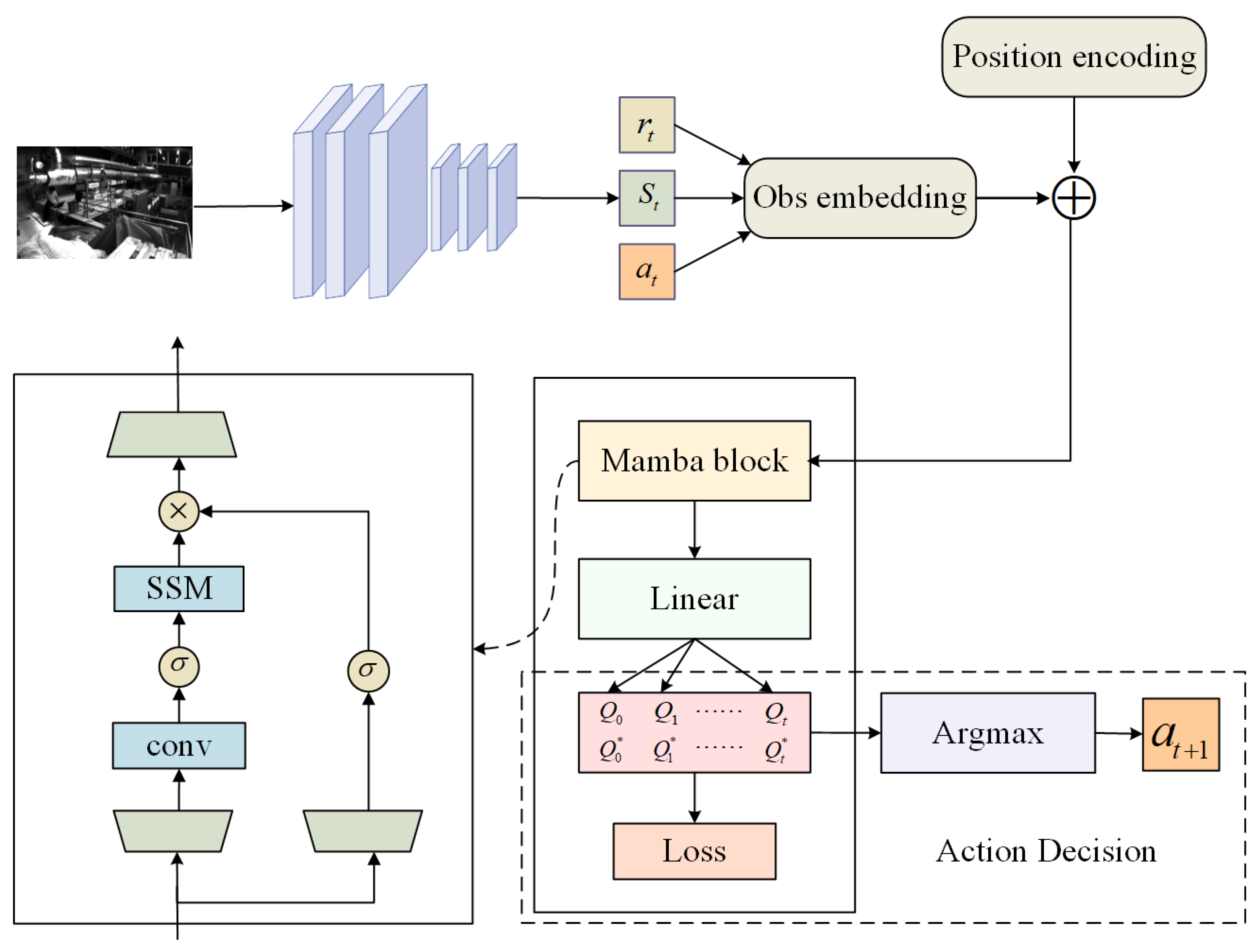
3.2. Mamba-DQN Agent

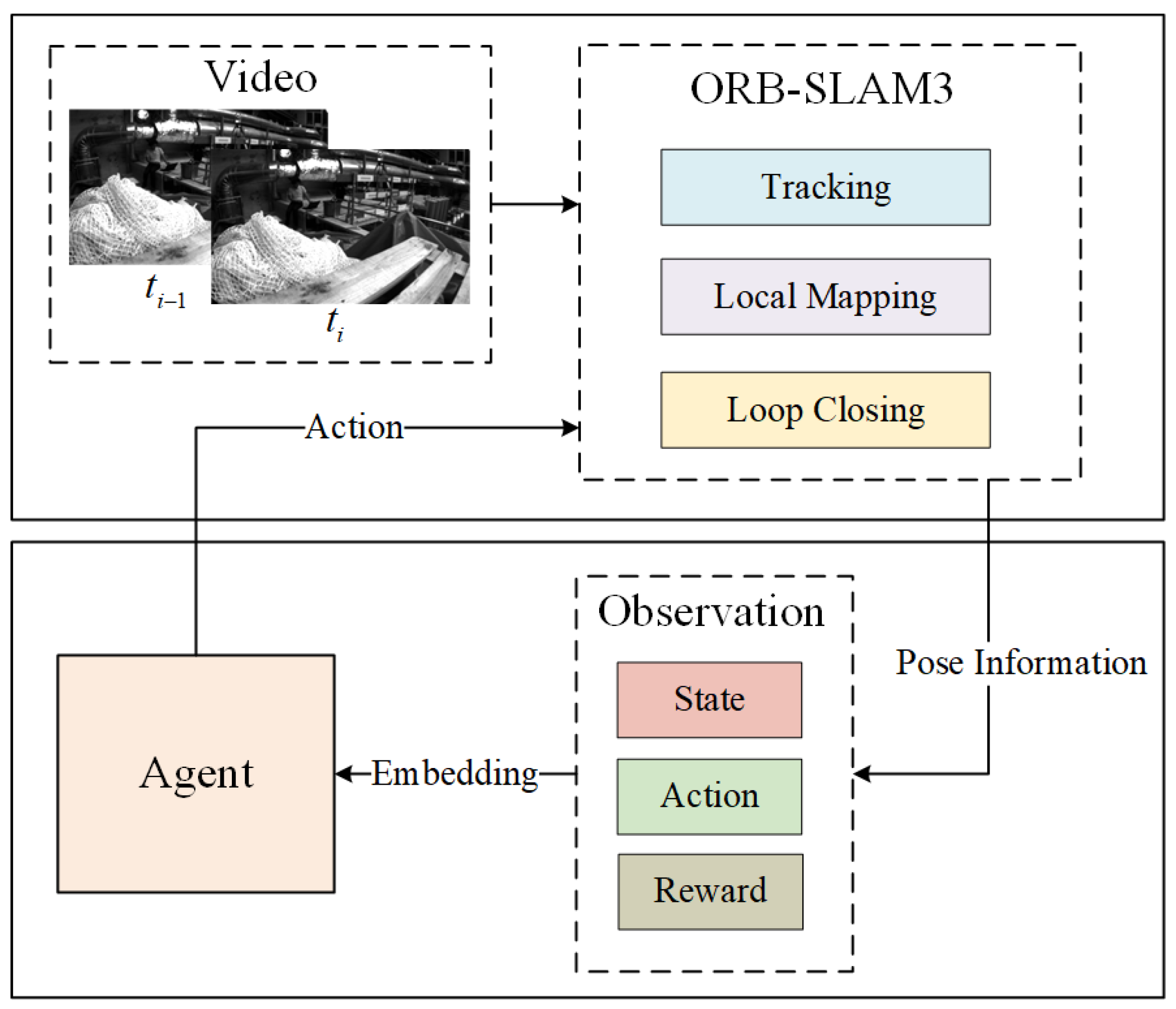
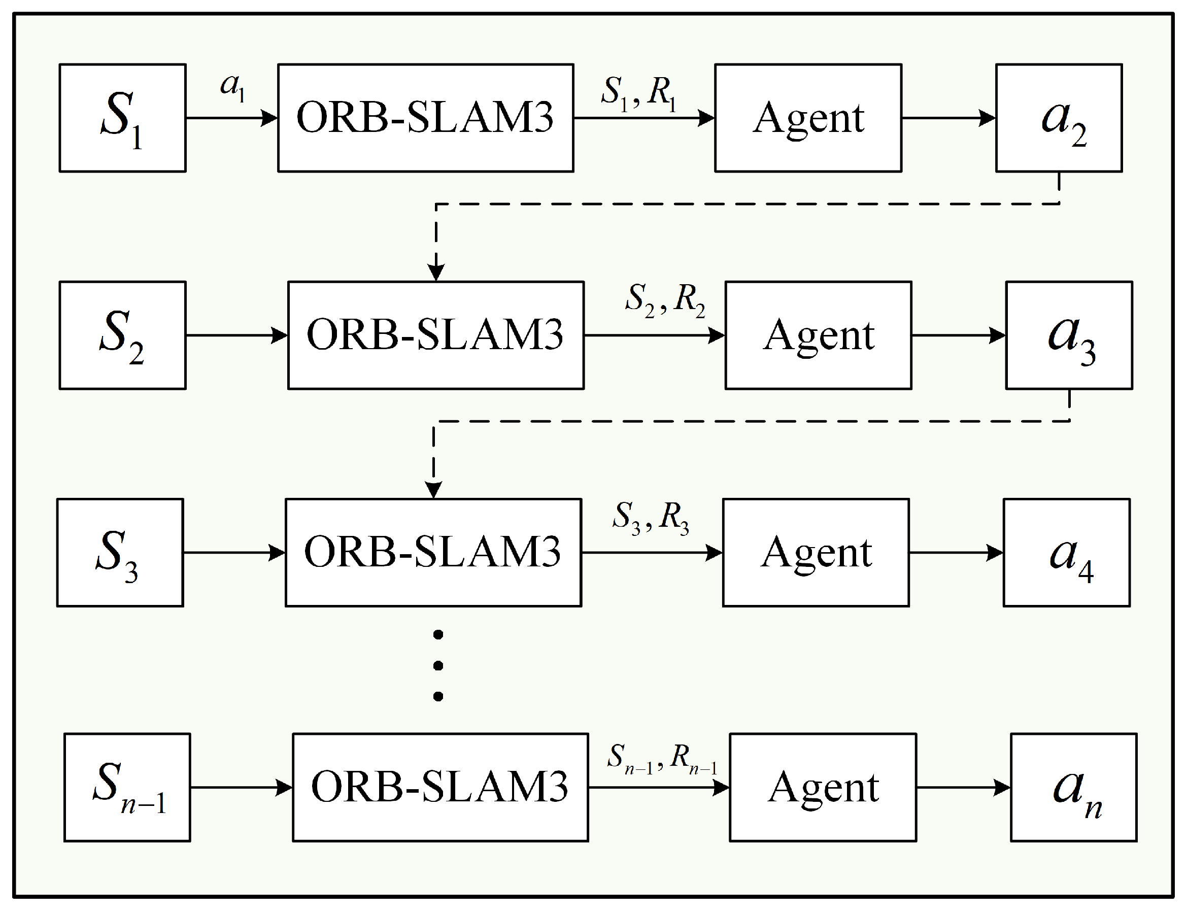
3.2.1. Mamba-DQN Interaction

The agent interacts with the environment and obtains corresponding O b s e r v a t i o n ( s t , a t , r t ) and combines multiple historical observations ( O t , O t + 1 O t + k ) into a historical experience U t : t + k . To facilitate the agent’s ability to more effectively learn the intrinsic relationships among historical observations and thereby select the optimal parameters for the environment, we encode and embed the absolute positions of prior experiences. As shown in Figure 2, The Mamba block is used as a learner to learn the historical observation trajectory. The DQN network makes action decisions and updates the loss based on the historical experience Q value. The loss function is defined as Equation (3):
As shown in Figure 3, ORB-SLAM3 is utilized as the environment for deep reinforcement learning, while DQN serves as the agent. At the beginning of the process, the agent selects an action (a predefined set of parameter values) and applies it to the environment. Upon receiving the action, the environment undergoes a state transition and returns the resulting reward R along with the updated state to the agent. Based on the received reward and the current state, the agent determines the next action. Through continuous iterations, the agent optimizes its action selection to identify the optimal parameter configuration.
The agent interacts with the environment and obtains the corresponding observation O b s e r v a t i o n ( s t , a t , r t ) . It then aggregates multiple historical observations ( O t , O t + 1 , , O t + k ) into a historical experience U t : t + k . To enhance the agent’s capability of learning intrinsic relationships among historical observations and improving parameter selection for the environment, we encode and embed the absolute positions of prior experiences.
As shown in Figure 2, the Mamba block is employed as a learner to capture the historical observation trajectory. The DQN network is responsible for making action decisions and updating the loss based on the historical experience Q value. The loss function is defined as Equation (3):
L o s s t + i θ = E π r t + i + ( m a x Q O t + i Q * O t + i ) 2
As shown in Algorithm 1, during observation, we not only focus in the current frame state of the agent but also use the historical observations ( O t , O t + 1 , , O t + k ) to form the context. This paper uses the linear time characteristics of the Mamba block to construct a Mamba learner to perform “experience learning” on the context.
Algorithm 1 obtains the Q values of all historical observations and uses these Q values to calculate the loss for network training. This context-based historical experience update method produces a more robust agent. As shown in Figure 2, when making action decisions, only the maximum Q value of the most recent observation is used for action decision-making.
Algorithm 1 Mamba-DQN
Require: 
Observation history ( O t , O t + 1 , , O t + k )
Ensure: 
Output  y i
1:
Function Observe:
2:
Observation synthesis: U t : t + k = ( O t , O t + 1 , , O t + k )
3:
for  i = t to t + k  do
4:
    A i ( D , N ) Parameter
5:
    B i s B ( U i )
6:
    C i s C ( U i )
7:
    i τ ( Parameter + s ( U i ) )
8:
    A ¯ i , B ¯ i discretize ( i , A i , B i )
9:
    y i SSM ( A ¯ i , B ¯ i , C i ) ( U i )
10:
end for
11:
return  y i
12:
Function Train:
13:
Sample history Observation ( O t , O t + 1 , , O t + k ) from replay buffer
14:
for  i = t to t + k  do
15:
    L o s s i ( θ ) E π [ r i + ( max Q ( O i ) Q * ( O i ) ) 2 ]
16:
end for
In the Mamba-DQN framework, the interaction mechanism between historical observations and the Q-network constitutes the core of efficient temporal modeling. At time step t, the agent obtains an observation sequence { O t k , O t k + 1 , , O t } from the environment and transforms it into high-dimensional representations using the observation embedding function ϕ o b s :
E o b s , t i = ϕ o b s ( O t i ) , i { 0 , 1 , , k }
Simultaneously, the corresponding action sequence is encoded through the action embedding function ϕ a c t :
E a c t , t i = ϕ a c t ( a t i ) , i { 1 , 2 , , k }
To ensure temporal consistency, a time shift operation is applied to the action embeddings:
E a c t , t i = E a c t , t i + 1 , if i { 1 , 2 , , k } 0 , if i = 0
Subsequently, the observation and action embeddings are concatenated with position encodings P t i to form complete temporal representations:
X t i = [ E a c t , t i E o b s , t i ] + P t i , i { 0 , 1 , , k }
where ⊕ denotes concatenation along the feature dimension. The full input sequence X = [ X t k , X t k + 1 , , X t ] is processed by the Mamba module. Mamba computes the hidden state at time step t i using a state-space model (SSM):
h t i = A ¯ t i · h t i 1 + B ¯ t i · X t i
y t i = C t i · h t i
where A ¯ t i and B ¯ t i are dynamically obtained through discretization:
A ¯ t i , B ¯ t i = discretize ( t i , A t i , B t i )
t i = τ ( Parameter + s ( X t i ) )
Finally, the Mamba-processed sequence Y = [ y t k , y t k + 1 , , y t ] is passed to the Q-network for policy learning, where the Q-values corresponding to the latest observation are used for decision-making:
a * = arg max a Q ( O t , a )
This mechanism enables Mamba-DQN to effectively model temporal dependencies, enhancing decision-making performance in complex environments.

3.2.2. Computational Analysis of Mamba-DQN

Based on the Mamba-DQN architecture described in the previous section, we analyze the computational overhead introduced by incorporating the Mamba model into the DQN framework.
(1)
Time Complexity Analysis
The time complexity of Mamba-DQN stems from several key components:
  • Sequence processing complexity:
A significant feature of Mamba is its linear time characteristics. For an observation sequence of length k, ( O t , O t + 1 , , O t + k ) , the processing time complexity is O ( k ) .
  • SSM computation complexity: for each time step, as shown in Equations (8)–(11), the computation includes the following:
  • State update: h t i = A ¯ t i · h t i 1 + B ¯ t i · X t i .
  • Output calculation: y t i = C t i · h t i .
These matrix operations have a time complexity related to the hidden state dimension d, resulting in an overall complexity of O ( d 2 k ) .
(2)
Memory Complexity Analysis
The memory overhead of Mamba-DQN consists of the following components:
  • Parameter storage: the parameter matrices in the Mamba module, including A i , B i , C i , and i , require storage space of approximately O ( d 2 ) , where d is the hidden state dimension.
  • Experience replay buffer: storing the historical observation sequence ( O t , O t + 1 , , O t + k ) requires O ( k · | O | ) memory, where | O | represents the size of a single observation.
  • Embedding representations: according to Equations (4)–(7), the model needs to store observation embeddings E o b s , action embeddings E a c t , and position encodings P, with a memory requirement of approximately O ( k · d ) .
  • Hidden States: the SSM computation process requires storing the hidden state h t i for each time step, with a memory requirement of O ( k · d ) .
In summary, the time complexity of Mamba-DQN is O ( d 2 k ) , and the memory complexity is O ( d 2 + k · | O | + k · d ) , where d is the hidden state dimension, k is the length of the historical observation sequence, and | O | is the size of a single observation. Compared with traditional DQN, Mamba-DQN introduces additional linear time complexity but achieves superior temporal modeling capabilities.

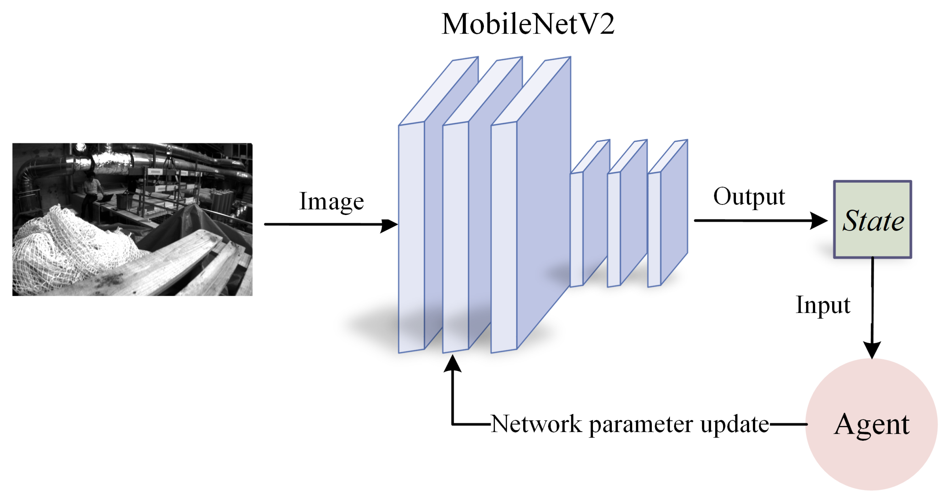
3.3. State Space Design

We employ the lightweight feature extractor MobileNetV2 [33] to derive features from video frames, thereby constructing the state space S t , as shown in Figure 4. Specifically, the processing of the state space in this study encompasses image preprocessing, deep convolutional separation, and feature mapping through reinforcement learning.
We define I as the original video frame, f as the process of feature extraction by the MobileNet network, and θ as the model parameters of MobileNet. The state processing process can be summarized as Equation (13):
S = f I , θ
Among them, θ is updated as the network parameters of the entire agent are updated, aiming to train a feature extractor that conforms to the video frame environment. The feature extractor is integrated into the agent so that the parameters of feature extraction and the decision parameters of the agent can share the same training process. As the agent persists in its learning within the environment, the network parameters of the feature extractor will be dynamically updated, enabling feature extraction to adapt fluidly to varying states and tasks, thereby enhancing its representational capabilities.

3.4. Reward Function Design

One of the goals of visual SLAM is to estimate camera motion and restore pose based on video frames, while traditional visual SLAM calculates camera pose based on information from adjacent frames. We leverage the feature of visual SLAM to construct a reinforcement learning reward module based on the absolute trajectory error between the predicted pose and the true pose of video frames and continuously provide feedback to the agent to enable the selected parameters (actions) to adapt to the current environment and obtain more accurate predicted poses, continuously reducing pose errors to maximize the expected reward.
The estimated pose of a certain frame in visual SLAM is P e s t i m a t e , and the true pose in the world coordinate system is P t r u e . We use the Umeyama algorithm [34] to calculate the root mean square error (RMSE) of the translational pose of P e s t i m a t e and P t r u e as the uncertainty G of the system. Our goal is to reduce the uncertainty of the system and improve the accuracy of pose estimation. The formula for calculating uncertainty is shown in Equation (14):
G = R M S E = i = 1 n ( P e s t i m a t e i P t r u e i ) 2 n
where n represents the frame rate and G = R M S E . Assuming the reward of the system is r, the calculation method of the reward function is shown in Equation (15):
r = log G

3.5. Action Space Design

The action space in the deep reinforcement learning module consists of the parameters in ORB-SLAM3. The selected parameters include the scale factor P 1 , the nearest neighbor threshold P 2 , and the number of pyramid levels P 3 . These three parameters play a crucial role in determining the accuracy of feature point extraction and the reliability of image matching.

3.5.1. Analysis of Parameters (Action) Selection

In visual SLAM systems, multi-scale pyramidal feature structures play a crucial role in feature extraction and matching, impacting localization accuracy and computational efficiency. The optimization of scale factors and pyramid levels significantly influences system adaptability. Studies [35,36] have demonstrated that selecting an appropriate scale factor enhances feature stability under varying environmental conditions, while the number of pyramid levels must balance computational cost and feature extraction accuracy [36,37,38,39,40]. Additionally, the nearest neighbor threshold affects feature matching robustness, requiring adaptive tuning to maintain stability in complex environments [9,41,42]. Collectively, these studies highlight the necessity of adaptive parameter optimization in SLAM, ensuring improved localization accuracy, feature robustness, and computational efficiency.
To evaluate the impact of different parameter settings on SLAM pose trajectory estimation, we conducted experiments and summarized the RMSE results of the ORB-SLAM3 algorithm on selected sequences from the EuRoC dataset in Table 1. The experimental results indicate that, for the same dataset sequences, different combinations of parameters P 1 , P 2 , and P 3 significantly affect SLAM localization accuracy and exhibit a certain degree of instability. Therefore, employing fixed parameter settings may not always ensure optimal performance across all scenarios, highlighting the potential importance of adaptive parameter tuning mechanisms in SLAM.

3.5.2. Definition of Action Space

To ensure that the reinforcement learning agent can sufficiently explore parameter combinations, we discretize the parameter space with the following value ranges:
P 1 [ 1.10 , 1.40 ] , P 2 [ 0.60 , 0.90 ] , P 3 [ 2 , 8 ]
The size of the action space is the product of the number of selectable values for each parameter (denoted as n 1 , n 2 , n 3 ), given by:
n = n 1 × n 2 × n 3
The action space is formally defined as
A = a 1 , a 2 , a 3 , , a n
where each action a i consists of a parameter tuple a i = ( P 1 , P 2 , P 3 ) , with i [ 1 , n ] .

4. Experiments

4.1. DataSets

In the experimental section, we used the Euroc MAV [43] and TUM-VI [44] datasets. The Euroc MAV dataset is a visual-inertial dataset collected by a micro aerial vehicle, which combines synchronized stereo images, inertial measurement unit (IMU) measurements, and ground truth information. The TUM-VI dataset is a visual-inertial dataset captured by handheld devices across diverse indoor environments, focusing on challenging scenarios such as rapid motion and fluctuating lighting conditions.
We designate the MH05 and V101 sequences from the Euroc MAV dataset as the training set, while the remaining sequences serve as the testing set. Concurrently, for the TUM-VI dataset, the Corridor4 and Room1 sequences are classified as training sets, with the other sequences allocated for testing purposes. In the experiment, the Umeyama algorithm was used for coordinate alignment, and the root mean square error (RMSE) between the predicted trajectory and the true trajectory of each sequence was calculated as the evaluation metric. In order to eliminate the uncertainty and randomness of the system, the final experimental results were taken as the median of 10 experimental results.

4.2. Analysis of Experimental Results

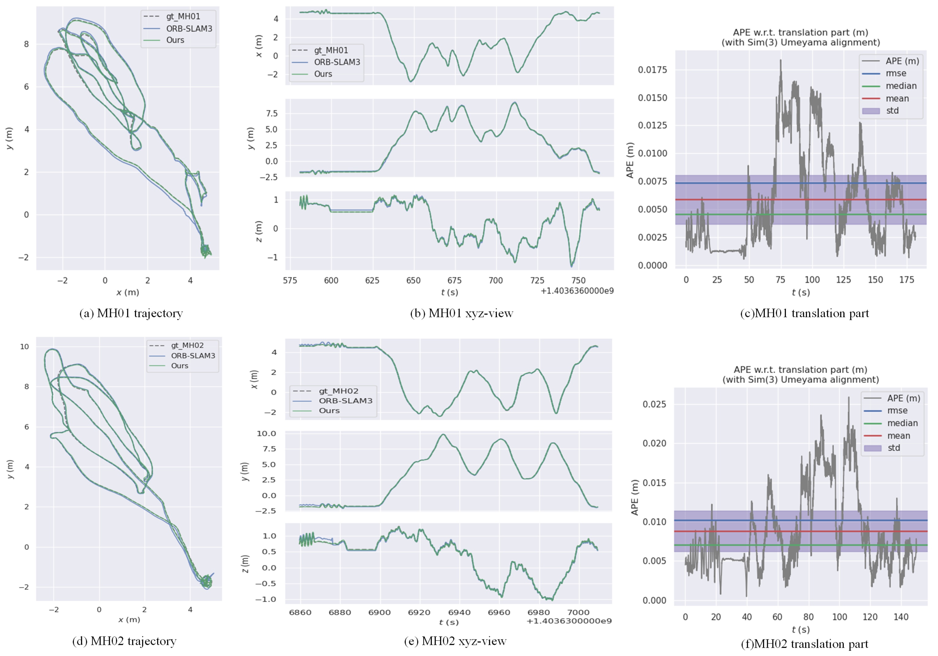
4.2.1. Result1: EUROC

The baseline methods compared in this section include traditional visual SLAM methods (SVO, ORB-SLAM3), deep learning-based visual SLAM methods (DDPG-SLAM), and end-to-end visual SLAM methods (DROID-SLAM). The experimental results are shown in Table 2.
Compared with traditional methods, our method shows better performance on multiple sequences of the dataset. Specifically, on MH01, MH02, MH03, MH04, and V202 sequences, the RMSE of our method is significantly lower than that of SVO and ORB-SLAM3 methods. Regarding the Vicon Room sequence, the experimental results of the proposed method demonstrate a relatively inadequate performance. This is because the sequence has complex visual environments and low image quality problems, such as blur noise, image distortion, and other unfavorable factors. However, in comparison with the SVO method, the experimental results of our method still demonstrate a certain level of robustness.
In comparison to deep learning and end-to-end visual SLAM methods, particularly on the Machine Hall sequences, our approach outperforms both DROID-SLAM and DDPG-SLAM, exhibiting a reduced RMSE. This enhancement is primarily attributable to the parameter adaptive algorithm introduced in this paper, which adeptly selects more appropriate parameters based on the specific characteristics of the scene, ultimately augmenting system performance. While the experimental outcomes of our method are somewhat less favorable compared with those of DROID-SLAM and DDPG-SLAM in the Vicon Room sequence, this discrepancy remains within an acceptable range given the inherent challenges and intricacies of the sequence itself. dAs shown in Figure 5, the experimental trajectory plot on the EUROC dataset.

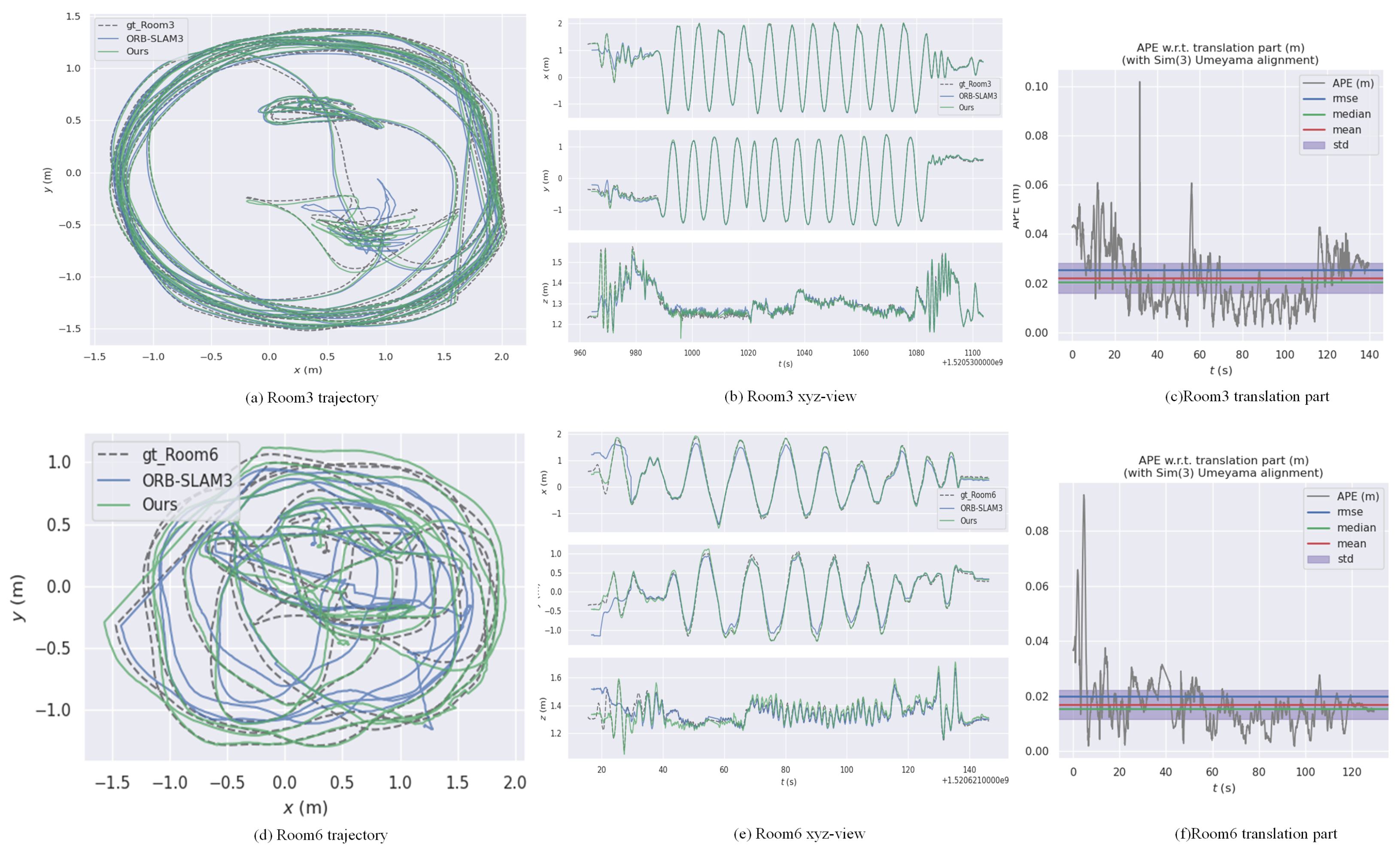
4.2.2. Result2: TUM-VI

Table 3 shows the results of different methods on the TUM-VI dataset. VINs-mono and ORB-SLAM3 are traditional visual SLAM methods, while DDPG-SLAM and SL-SLAM [46] are deep-learning based visual SLAM methods.
Based on the data presented in Table 3, the proposed method demonstrates a reduced RMSE on both the Corridor and Room sequence datasets. The RMSE for 66.7% of the sequences is lower than that of alternative methods, with a notable reduction of approximately twofold in RMSE for the Corridor1 and Room6 sequences. Our method demonstrates improved experimental results on the Corridor5 sequence when compared with the VINS-mono method, yet it falls short of surpassing the performance of the remaining three methods. As shown in Figure 6, the experimental trajectory plot on the TUM-VI dataset.
We conducted tests in more challenging scenarios of the TUM-VI dataset, including Outdoors, Slides, and Magistrale, as shown in Table 4. Taking “magistrale1” and “slides1” as examples, our method demonstrates lower RMSE values in these complex scenarios, 0.81 and 0.53, respectively, outperforming both VINS-mono and ORB-SLAM3. However, it is worth noting that in the “magistrale3” sequence, VINS-mono performs better, with an RMSE of 0.40, surpassing both ORB-SLAM3 and our method.

4.2.3. Result3: Memory Usage and Time Performance

For the purpose of evaluating the efficiency of the method introduced in this article, we carried out comparative experiments focusing on both system memory usage and execution time, using ORB-SLAM3 and DDPG-SLAM methods as comparative baselines.
All tests were conducted on hardware equipped with an NVIDIA 4060 8 GB (NVIDIA Corporation, Santa Clara, CA, USA) graphics card and an Intel(R) Core(TM) i7-10700 CPU@2.90 GHz (NVIDIA Corporation, Santa Clara, CA, USA). The memory usage details are summarized in Table 5.
In terms of execution time, a comparative analysis was conducted among ORB-SLAM3, DDPG-SLAM, and the proposed Mamba-based SLAM method. The results in Table 6 demonstrate that the execution time of the proposed method is generally comparable to that of ORB-SLAM3 across multiple test sequences, such as MH01, MH04, V202, and Room2. For instance, in the MH01 sequence, the time difference between the two methods is merely 1 s, which is negligible, indicating that the proposed method maintains a real-time performance similar to ORB-SLAM3. Furthermore, compared with DDPG-SLAM, the Mamba-based method exhibits shorter execution times in nearly all test sequences. As shown in Table 6, in the MH01 sequence, the proposed method runs 3 s faster than DDPG-SLAM, while in the MH02 sequence, it achieves a 20-s reduction in execution time, demonstrating a significant advantage in computational efficiency.
Overall, the introduction of the Mamba component leads to an increase in memory usage; however, this does not result in a significant rise in execution time. On the contrary, in some cases, it achieves higher efficiency than DDPG-SLAM. These findings suggest that the Mamba component effectively enhances computational efficiency while maintaining real-time performance within a reasonable resource overhead.

4.2.4. Result4: Ablation Experiment

(1) 
Ablation Study on Different Observation Modules
To verify the effectiveness of the Mamba historical observer, an ablation experiment was designed in this section, consisting of three parts: the no-agent module, the Mamba observation module, and the observation module combined with different reinforcement learning algorithms and the Attention mechanism. Partial experimental results are presented in Table 7.
The data in Table 7 demonstrate that the proposed method achieves an optimal trade-off between localization accuracy and the real-time performance of the SLAM system. In the absence of the Mamba module, the DQN method achieves a lower RMSE of 0.013 on the MH01 dataset compared with the agent-free method, which has an RMSE of 0.016. However, there is no significant improvement in computational time.
Upon incorporating the Mamba module, our method shows superior performance across multiple datasets. On the MH01 dataset, the RMSE of our method is 0.007, which is comparable to that of A3C+Mamba (0.007) but with a slight advantage in computational time. On the V202 dataset, our method achieves an RMSE of 0.019, slightly better than A3C+Mamba’s 0.020, with identical computational time. When compared with the “DQN + Attention” methods, including DRQN and DQN+Transformer, our method outperforms both in terms of localization accuracy and runtime. For instance, on the Room5 dataset, the RMSE of our method is 0.009, significantly lower than DRQN’s 0.010 and DQN+Transformer’s 0.024, while the runtime is identical to that of DRQN. In conclusion, the proposed method ensures high localization accuracy while significantly improving the real-time performance of the SLAM system, demonstrating stronger adaptability and superior performance compared with existing approaches. Figure 7 shows the trajectory comparison of different agent methods.
(2) 
Ablation Study on Historical Observation Window Size
In this experiment, we set BatchSize = 30 as the baseline configuration based on the real-time frame rate (approximately 30 frames per second) of ORB-SLAM3 on our testing platform and compared it with BatchSize = 15 and BatchSize = 60 to evaluate the impact of different historical observation window sizes on system performance. As shown in Table 8, BatchSize = 30 demonstrates significant advantages in both accuracy and efficiency. On the MH01 dataset, BatchSize = 30 achieves an RMSE of 0.007, outperforming BatchSize = 15 with an RMSE of 0.028 and showing comparable performance to BatchSize = 60 with an RMSE of 0.008 while reducing computation time by approximately 12% compared with BatchSize = 60 (220 s vs. 249 s). Similarly, on the MH02 dataset, BatchSize = 30 maintains an RMSE of 0.010, slightly lower than BatchSize = 60’s 0.009, while decreasing processing time from 185 s to 163 s.
In the V202 dataset tests, BatchSize = 30 and BatchSize = 60 achieved identical RMSE values of 0.019, yet BatchSize = 30 required significantly less processing time (123 s vs. 135 s). For the Corridor2 dataset, while BatchSize = 60 showed a marginally better RMSE of 0.012 compared with BatchSize = 30’s 0.014, this came at a substantial computational cost, with processing time increasing from 373 s to 426 s. Similar patterns were observed in the Corridor5 dataset, where BatchSize = 30 matched the accuracy of BatchSize = 60 (both with RMSE of 0.047) while reducing processing time by approximately 9.4% (349 s vs. 385 s).
In tests with the Room5 dataset, BatchSize = 30 maintained the same accuracy as BatchSize = 60 (both with RMSE of 0.009) while significantly reducing computational overhead (156 s vs. 186 s). This trend is evident across most test scenarios, indicating that larger BatchSize values often lead to diminishing returns in accuracy while substantially increasing computational demands, whereas BatchSize = 30 provides an optimal trade-off between precision and efficiency.
In conclusion, BatchSize = 30, which corresponds to the system’s real-time operational frame rate, achieves the optimal balance between accuracy and efficiency, making it the ideal configuration for our system.

5. Discussion

In this study, we propose an innovative solution to the adaptive parameter adjustment challenge in visual SLAM by leveraging the deep Mamba-Q network. By transforming the traditionally complex and manual parameter tuning process into a policy learning task, our approach offers a more systematic and automated framework for optimizing system performance. The integration of the Mamba historical observer with the deep reinforcement learning agent enables seamless alignment of the Mamba-DQN algorithm with the ORB-SLAM3 system, resulting in enhanced adaptability and performance in dynamic environments. This reinterpretation of parameter adaptation as an action decision-making problem within the reinforcement learning paradigm underscores the potential of deep learning techniques to enhance the capabilities of visual SLAM systems.

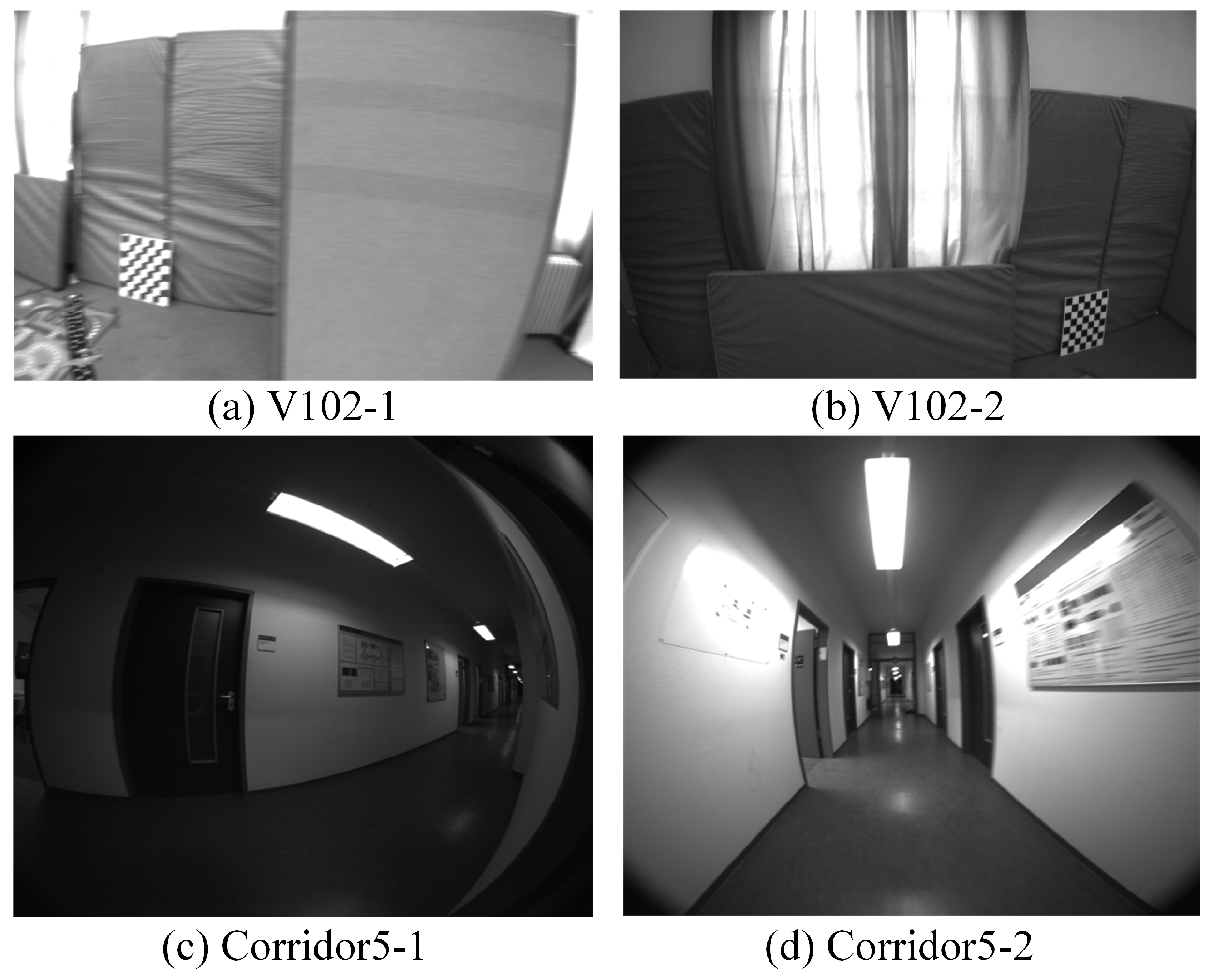
Failure Case Analysis

Our method exhibited suboptimal performance in several specific scenarios, particularly in the V102, V201, and Corridor5 sequences. In the V102 sequence, the RMSE of our approach was 0.038 m, significantly higher than that of ORB-SLAM3 (0.015 m) and DROID-SLAM (0.012 m). Similarly, in the V201 sequence, our method achieved an RMSE of 0.120 m, marking the largest performance gap across all tested sequences when compared with the baseline methods.
The primary factors contributing to these failures are as follows:
  • Scene complexity: In the V102 and V201 sequences, rapid camera motion combined with complex lighting conditions led to failures in the Mamba historical observer’s learning process, preventing it from effectively updating the observation model, as shown in Figure 8a,b.
  • Feature sparsity: In the Corridor5 sequence, our method achieved an RMSE of 0.040 m, while DDPG-SLAM achieved 0.010 m and SL-SLAM 0.009 m. The corridor environment, characterized by repetitive textures and relatively flat walls, resulted in suboptimal feature extraction and tracking. Additionally, image distortion further exacerbated this issue, leading to the Mamba historical observer’s failure to properly learn from historical experiences. These issues are illustrated in Figure 8c,d, where distortion is particularly evident during the feature extraction process.
These failure cases highlight key directions for future research. Firstly, there is a need to develop more robust mechanisms to distinguish between scenarios that require dynamic parameter adaptation and those where default parameters suffice, thereby improving the system’s adaptability. Secondly, incorporating more advanced historical experience learning methods could enhance the Mamba model’s ability to learn effectively in feature-scarce and rapidly changing environments, thus improving decision-making accuracy and stability. These improvements would contribute to the overall performance enhancement of SLAM systems in complex scenarios.

6. Conclusions

In conclusion, this paper presents a novel approach to the adaptive parameter tuning problem in visual SLAM through the use of deep Mamba-Q network reinforcement learning. The proposed method transforms the complex task of parameter adjustment into a policy learning challenge, successfully integrating the Mamba-DQN algorithm with ORB-SLAM3. Experimental results show that our approach outperforms baseline methods in terms of pose estimation accuracy and operational efficiency for over 50% of the test sequences.
Despite these promising results, the method still has room for improvement. The impact of environmental factors such as lighting, shadows, and blur needs to be better accounted for, especially in challenging sequences like V and Corridor5. Future work should focus on optimizing the model to handle these factors, improving its adaptability and robustness in a wider range of scenarios.

Author Contributions

Conceptualization, X.M. and C.H.; methodology, X.M. and C.H.; software, X.M. and W.W.; validation, X.M.; formal analysis, X.M.; investigation, X.M. and X.H.; resources, X.M. and X.H.; data curation, X.M.; writing—original draft preparation, X.M.; writing—review and editing, X.M. and C.H.; visualization, X.M. and X.H.; supervision, X.M. and C.H.; project administration, X.M. and C.H.; funding acquisition, C.H. All authors have read and agreed to the published version of the manuscript.

Funding

This research was funded by the National Natural Science Foundation of China (grant number 62162007) and the Natural Science Foundation of Guizhou Province (grant number QianKeHeJiChu-ZK[2024]YiBan079).

Institutional Review Board Statement

Not applicable.

Informed Consent Statement

Not applicable.

Data Availability Statement

The data supporting the reported results in this study are publicly available. The EuRoC MAV dataset can be accessed at https://projects.asl.ethz.ch/datasets/doku.php?id=kmavvisualinertialdatasets (accessed on 6 September 2024). The TUM-VI dataset is available at https://vision.in.tum.de/data/datasets/visual-inertial-dataset (accessed on 6 September 2024). Both datasets are open and do not require an application for access. We have placed the code for this study at Github: https://github.com/Xuboma/Mamba-DQN-SLAM.git (accessed on 28 September 2024).

Conflicts of Interest

The authors declare no conflicts of interest.

Abbreviations

The following abbreviations are used in this manuscript:
SLAMSimultaneous Localization and Mapping
ATEAbsolute Trajectory Error
DQNDeep Q-Network
ARAugmented Reality
VRVirtual Reality
CNNConvolutional Neural Network
DDPGDeep Deterministic Policy Gradient
3DThree-dimensional
ORBOriented fast and Rotated Brief
RMSERoot Mean Square Error
DDQNDouble Deep Q-Network
A3CAsynchronous Advantage Actor-Critic
PPOProximal Policy Optimization
DRQNDeep Recurrent Q-Network

References

  1. Teed, Z.; Lipson, L.; Deng, J. Deep patch visual odometry. In Proceedings of the Advances in Neural Information Processing Systems, New Orleans, LA, USA, 10–16 December 2023; Volume 36. [Google Scholar]
  2. Chen, Y.; Inaltekin, H.; Gorlatova, M. AdaptSLAM: Edge-Assisted Adaptive SLAM with Resource Constraints via Uncertainty Minimization. In Proceedings of the IEEE INFOCOM 2023–IEEE Conference on Computer Communications, New York, NY, USA, 17–20 May 2023; pp. 1–10. [Google Scholar]
  3. Messikommer, N.; Cioffi, G.; Gehrig, M.; Scaramuzza, D. Reinforcement Learning Meets Visual Odometry. In Proceedings of the European Conference on Computer Vision (ECCV), Milan, Italy, 29 September–4 October 2024; pp. 76–92. [Google Scholar]
  4. Khalufa, A.; Riley, G.; Luján, M. A dynamic adaptation strategy for energy-efficient keyframe-based visual SLAM. In Proceedings of the International Conference on Parallel and Distributed Processing Techniques and Applications (PDPTA), Las Vegas, NV, USA, 24–27 June 2019; Arabnia, H.R., Ed.; CSREA Press: Las Vegas, NV, USA, 2019; pp. 3–10. [Google Scholar]
  5. Kuo, J.; Muglikar, M.; Zhang, Z.; Scaramuzza, D. Redesigning SLAM for arbitrary multi-camera systems. In Proceedings of the 2020 IEEE International Conference on Robotics and Automation (ICRA), Virtual Conference, 31 May–31 August 2020; pp. 2116–2122. [Google Scholar]
  6. Gao, W.; Huang, C.; Xiao, Y.; Huang, X. Parameter adaptive of visual SLAM based on DDPG. J. Electron. Imaging 2023, 32, 053027. [Google Scholar] [CrossRef]
  7. Mur-Artal, R.; Montiel, J.M.M.; Tardos, J.D. ORB-SLAM: A versatile and accurate monocular SLAM system. IEEE Trans. Robot. 2015, 31, 1147–1163. [Google Scholar] [CrossRef]
  8. Aglave, P.; Kolkure, V.S. Implementation of high performance feature extraction method using Oriented FAST and Rotated BRIEF algorithm. Int. J. Res. Eng. Technol. 2015, 4, 394–397. [Google Scholar]
  9. Mur-Artal, R.; Tardós, J.D. ORB-SLAM2: An open-source SLAM system for monocular, stereo, and RGB-D cameras. IEEE Trans. Robot. 2017, 33, 1255–1262. [Google Scholar] [CrossRef]
  10. Campos, C.; Elvira, R.; Rodríguez, J.J.G.; Montiel, J.M.; Tardós, J.D. ORB-SLAM3: An accurate open-source library for visual, visual–inertial, and multimap SLAM. IEEE Trans. Robot. 2021, 37, 1874–1890. [Google Scholar] [CrossRef]
  11. Tateno, K.; Tombari, F.; Laina, I.; Navab, N. CNN-SLAM: Real-time dense monocular SLAM with learned depth prediction. In Proceedings of the IEEE Conference on Computer Vision and Pattern Recognition (CVPR), Honolulu, HI, USA, 21–26 July 2017; pp. 6243–6252. [Google Scholar]
  12. Teed, Z.; Deng, J. Droid-SLAM: Deep visual SLAM for monocular, stereo, and RGB-D cameras. Adv. Neural Inf. Process. Syst. 2021, 34, 16558–16569. [Google Scholar]
  13. Bhowmik, A.; Gumhold, S.; Rother, C.; Brachmann, E. Reinforced feature points: Optimizing feature detection and description for a high-level task. In Proceedings of the IEEE/CVF Conference on Computer Vision and Pattern Recognition, Seattle, WA, USA, 13–19 June 2020; pp. 4948–4957. [Google Scholar]
  14. Chandio, Y.; Khan, M.A.; Selialia, K.; Garcia, L.; DeGol, J.; Anwar, F.M. A neurosymbolic approach to adaptive feature extraction in SLAM. In Proceedings of the 2024 IEEE/RSJ International Conference on Intelligent Robots and Systems (IROS), Abu Dhabi, United Arab Emirates, 14–18 October 2024; pp. 4941–4948. [Google Scholar]
  15. Zhou, L.; Wang, M.; Zhang, X.; Qin, P.; He, B. Adaptive SLAM methodology based on simulated annealing particle swarm optimization for AUV navigation. Electronics 2023, 12, 2372. [Google Scholar] [CrossRef]
  16. Jia, Y.; Luo, H.; Zhao, F.; Jiang, G.; Li, Y.; Yan, J.; Jiang, Z.; Wang, Z. Lvio-fusion: A self-adaptive multi-sensor fusion SLAM framework using actor-critic method. In Proceedings of the 2021 IEEE/RSJ International Conference on Intelligent Robots and Systems (IROS), Prague, Czech Republic, 27 September–1 October 2021; pp. 286–293. [Google Scholar]
  17. Mnih, V.; Kavukcuoglu, K.; Silver, D.; Rusu, A.A.; Veness, J.; Bellemare, M.G.; Graves, A.; Riedmiller, M.; Fidjeland, A.K.; Ostrovski, G.; et al. Human-level control through deep reinforcement learning. Nature 2015, 518, 529–533. [Google Scholar] [CrossRef]
  18. Silver, D.; Lever, G.; Heess, N.; Degris, T.; Wierstra, D.; Riedmiller, M. Deterministic policy gradient algorithms. In Proceedings of the International Conference on Machine Learning, Beijing, China, 21–26 June 2014; Xing, E.P., Jebara, T., Eds.; JMLR.org: Beijing, China, 2014; pp. 387–395. [Google Scholar]
  19. Hausknecht, M.; Stone, P. Deep recurrent q-learning for partially observable MDPs. In Proceedings of the 2015 AAAI Fall Symposium Series, Arlington, VA, USA, 12–14 November 2015. [Google Scholar]
  20. Fujimoto, S.; Hoof, H.; Meger, D. Addressing function approximation error in actor-critic methods. In Proceedings of the 2018 International Conference on Machine Learning (ICML), Stockholm, Sweden, 10–15 July 2018; pp. 1587–1596. [Google Scholar]
  21. Vaswani, A. Attention is all you need. Adv. Neural Inf. Process. Syst. 2017. [Google Scholar]
  22. Parisotto, E.; Song, F.; Rae, J.; Pascanu, R.; Gulcehre, C.; Jayakumar, S.; Jaderberg, M.; Kaufman, R.L.; Clark, A.; Noury, S.; et al. Stabilizing transformers for reinforcement learning. In Proceedings of the International Conference on Machine Learning, Vienna, Austria, 12–18 July 2020; pp. 7487–7498. [Google Scholar]
  23. Chen, L.; Lu, K.; Rajeswaran, A.; Lee, K.; Grover, A.; Laskin, M.; Abbeel, P.; Srinivas, A.; Mordatch, I. Decision transformer: Reinforcement learning via sequence modeling. Adv. Neural Inf. Process. Syst. 2021, 34, 15084–15097. [Google Scholar]
  24. Hu, S.; Shen, L.; Zhang, Y.; Tao, D. Graph decision transformer. arXiv 2023, arXiv:2303.03747. [Google Scholar]
  25. Yamagata, T.; Khalil, A.; Santos-Rodriguez, R. Q-learning decision transformer: Leveraging dynamic programming for conditional sequence modelling in offline RL. In Proceedings of the 40th International Conference on Machine Learning, Hawaii Convention Center, Honolulu, HI, USA, 23–29 July 2023; pp. 38989–39007. [Google Scholar]
  26. Esslinger, K.; Platt, R.; Amato, C. Deep Transformer Q-Networks for Partially Observable Reinforcement Learning. arXiv 2022, arXiv:2206.01078. [Google Scholar]
  27. Chebotar, Y.; Vuong, Q.; Hausman, K.; Xia, F.; Lu, Y.; Irpan, A.; Kumar, A.; Yu, T.; Herzog, A.; Pertsch, K.; et al. Q-transformer: Scalable offline reinforcement learning via autoregressive q-functions. In Proceedings of the Conference on Robot Learning, Atlanta, GA, USA, 6–9 November 2023; pp. 3909–3928. [Google Scholar]
  28. Hu, S.; Shen, L.; Zhang, Y.; Chen, Y.; Tao, D. On transforming reinforcement learning with transformers: The development trajectory. IEEE Trans. Pattern Anal. Mach. Intell. 2024. [Google Scholar] [CrossRef] [PubMed]
  29. Wang, Z.; Zhang, L.; Wu, W.; Zhu, Y.; Zhao, D.; Chen, C. Meta-DT: Offline Meta-RL as Conditional Sequence Modeling with World Model Disentanglement. Adv. Neural Inf. Process. Syst. 2025, 37, 44845–44870. [Google Scholar]
  30. Kalman, R.E. A new approach to linear filtering and prediction problems. Trans. Asme J. Basic Eng. 1960, 82, 35–45. [Google Scholar] [CrossRef]
  31. Sherstinsky, A. Fundamentals of recurrent neural network (RNN) and long short-term memory (LSTM) network. Phys. Nonlinear Phenom. 2020, 404, 132306. [Google Scholar] [CrossRef]
  32. Dao, T.; Gu, A. Transformers are SSMs: Generalized Models and Efficient Algorithms Through Structured State Space Duality. In Proceedings of the Forty-First International Conference on Machine Learning (ICML), Vienna, Austria, 21–27 July 2024; pp. 1–10. [Google Scholar]
  33. Sandler, M.; Howard, A.; Zhu, M.; Zhmoginov, A.; Chen, L.C. MobileNetV2: Inverted residuals and linear bottlenecks. In Proceedings of the IEEE Conference on Computer Vision and Pattern Recognition (CVPR), Salt Lake City, UT, USA, 18–22 June 2018; pp. 4510–4520. [Google Scholar]
  34. Umeyama, S. Least-squares estimation of transformation parameters between two point patterns. IEEE Trans. Pattern Anal. Mach. Intell. 1991, 13, 376–380. [Google Scholar] [CrossRef]
  35. Tang, L.; Tang, W.; Qu, X.; Han, Y.; Wang, W.; Zhao, B. A Scale-Aware Pyramid Network for Multi-Scale Object Detection in SAR Images. Remote Sens. 2022, 14, 973. [Google Scholar] [CrossRef]
  36. Zhou, X.; Zhang, L. SA-FPN: An effective feature pyramid network for crowded human detection. Appl. Intell. 2022, 52, 12556–12568. [Google Scholar] [CrossRef]
  37. Yang, X.; Liu, L.; Wang, N.; Gao, X. A two-stream dynamic pyramid representation model for video-based person re-identification. IEEE Trans. Image Process. 2021, 30, 6266–6276. [Google Scholar] [CrossRef]
  38. Yu, Y.; Zhang, Y.; Cheng, Z.; Song, Z.; Tang, C. Multi-scale spatial pyramid attention mechanism for image recognition: An effective approach. Eng. Appl. Artif. Intell. 2024, 133, 108261. [Google Scholar] [CrossRef]
  39. Kumar, A.; Park, J.; Behera, L. High-speed stereo visual SLAM for low-powered computing devices. IEEE Robot. Autom. Lett. 2023, 9, 499–506. [Google Scholar] [CrossRef]
  40. Guo, X.; Lyu, M.; Xia, B.; Zhang, K.; Zhang, L. An Improved Visual SLAM Method with Adaptive Feature Extraction. Appl. Sci. 2023, 13, 10038. [Google Scholar] [CrossRef]
  41. DeTone, D.; Malisiewicz, T.; Rabinovich, A. SuperPoint: Self-Supervised Interest Point Detection and Description. In Proceedings of the IEEE Conference on Computer Vision and Pattern Recognition (CVPR), Salt Lake City, UT, USA, 18–22 June 2018; pp. 1–10. [Google Scholar]
  42. Cai, Z.; Ou, Y.; Ling, Y.; Dong, J.; Lu, J.; Lee, H. Feature Detection and Matching with Linear Adjustment and Adaptive Thresholding. IEEE Access 2020, 8, 189735–189746. [Google Scholar] [CrossRef]
  43. Burri, M.; Nikolic, J.; Gohl, P.; Schneider, T.; Rehder, J.; Omari, S.; Achtelik, M.; Siegwart, R. The EuRoC micro aerial vehicle datasets. Int. J. Robot. Res. 2016, 35, 103–111. [Google Scholar] [CrossRef]
  44. TUM Visual-Inertial Dataset. Available online: https://cvg.cit.tum.de/data/datasets/visual-inertial-dataset (accessed on 6 September 2024).
  45. Forster, C.; Pizzoli, M.; Scaramuzza, D. SVO: Fast semi-direct monocular visual odometry. In Proceedings of the 2014 IEEE International Conference on Robotics and Automation (ICRA), Hong Kong, China, 31 May–7 June 2014; pp. 15–22. [Google Scholar]
  46. Xiao, Z.; Li, S. SL-SLAM: A robust visual-inertial SLAM based deep feature extraction and matching. arXiv 2024, arXiv:2405.03413. [Google Scholar]
  47. Qin, T.; Li, P.; Shen, S. VINS-Mono: A robust and versatile monocular visual-inertial state estimator. IEEE Trans. Robot. 2018, 34, 1004–1020. [Google Scholar] [CrossRef]
Figure 1. Mamba-DQN SLAM framework.
Applsci 15 02950 g001
Figure 2. Mama-DQN agent.
Applsci 15 02950 g002
Figure 3. Agent–environment interaction.
Applsci 15 02950 g003
Figure 4. State processing flow.
Applsci 15 02950 g004
Figure 5. Comparison of pose trajectories in some sequences of the Euroc MAV dataset. (a,d) show the trajectory estimation results for the MH01 and MH02 sequences, where our method (green) exhibits reduced drift compared with the baseline method (blue). (b,e) highlight the details of trajectory alignment, demonstrating that our method achieves higher accuracy in key trajectory segments. (c,f) illustrate the distribution of absolute pose errors, indicating that our method maintains lower error levels.
Applsci 15 02950 g005
Figure 6. Comparison of pose trajectories in some sequences of the TUM-VI dataset. (a,d) compare the trajectories of Room3 and Room6, where our method (green) demonstrates reduced drift compared with the baseline method (blue). (b,e) focus on the details of orbit alignment, showing that our method provides higher accuracy in key trajectory segments. (c,f) present the distribution of absolute attitude errors, indicating that our method maintains lower error levels.
Applsci 15 02950 g006
Figure 7. Comparison of trajectories from different methods on the MH01 sequence. The red line represents the trajectory of the Mamba-DQN observed agent, the green line represents the DQN agent trajectory, and the blue line represents the original ORB-SLAM3 trajectory. As seen in the figure, the trajectory drift error of Mamba-DQN is closest to the true trajectory, while the maximum drift error of the original ORB-SLAM3 is the farthest from the true trajectory.
Applsci 15 02950 g007
Figure 8. Partial datasets from V102 and Corridor5.
Applsci 15 02950 g008
Table 1. SLAM localization results on different fixed parameters. R M S E / m .
Parameters ( P 1 - P 2 - P 3 )MH01MH02MH03MH04
1.1-0.9-80.0100.0240.0260.143
1.3-0.7-70.0310.0870.0590.058
1.4-0.9-90.0270.0240.0420.072
1.2-0.6-90.0180.0630.0860.146
1.2-0.8-80.0100.0690.0570.055
1.2-0.8-40.0150.0190.0430.084
Table 2. Absolute trajectory error of EUROC MAV dataset. R M S E / m .
SVO [45]ORB-SLAM3DDPG-SLAM [6]DROID-SLAM [12]Ours
MH010.1000.0160.0080.0130.007
MH020.1200.0270.0110.0140.010
MH030.4100.0280.0230.0220.018
MH040.4200.1380.0110.0430.007
V1020.2100.0150.0160.0120.038
V2010.1100.0230.0210.0170.120
V2020.1100.0290.0220.0130.019
Table 3. Absolute trajectory error of TUM-VI dataset. R M S E / m .
VINS-Mono [47]ORB-SLAM3DDPG-SLAM [6]SL-SLAM [46]Ours
Corridor10.6300.0400.0210.0860.011
Corridor20.9500.0200.0190.0620.014
Corridor31.5600.0310.2000.0390.018
Corridor50.1700.0300.0100.0090.040
Room20.0700.0200.028-0.028
Room30.1100.0400.030-0.025
Room40.0400.0100.020-0.046
Room50.2000.0200.010-0.009
Room60.0800.040--0.019
Table 4. Absolute trajectory error of TUM-VI dataset in challenging scenarios. R M S E / m .
VINS-Mono [47]ORB-SLAM3Ours
magistrale12.191.130.81
magistrale23.110.630.49
magistrale30.404.890.98
outdoors174.9670.7930.62
outdoors2133.4614.9812.92
outdoors336.9939.6326.87
slides10.680.970.53
slides20.841.060.42
slides30.690.690.43
Table 5. Comparison of GPU memory usage.
Agent TypeMemory Usage (MB)
DQN with Mamba728.4
DQN Without Mamba529.6
Table 6. Comparison of partial sequence system running time. S e c o n d / s ↓.
ORB_SLAM3DDPG_SLAM [6]Ours
MH01199223220
MH02162183163
MH04106118107
V202123137123
Corridor2366381373
Corridor5344349349
Room2158171158
Room5154168156
Table 7. Ablation Comparison experiment on different agents. R M S E and T i m e .
AgentMH01V202Corridor2Room5
RMSE Time RMSE Time RMSE Time RMSE Time
Without Mamba
-0.0162200.0291230.0403740.020154
DQN0.0132210.0291240.0143750.026156
DRL + Mamba
DDQN + Mamba0.0152240.0211230.0123740.013156
A3C + Mamba0.0072280.0201280.0103750.008157
PPO + Mamba0.0102320.0181320.0093840.009158
Ours0.0072200.0191230.0113730.009156
DQN + Attention
DRQN0.0122420.0201340.0133950.010169
DQN + Transformer0.0082520.0201460.0154000.024177
Table 8. Ablation study on different historical observation window sizes.
DatasetBatchSize = 15BatchSize = 30BatchSize = 60
RMSETime (s)RMSETime (s)RMSETime (s)
MH010.0282200.0072200.008249
MH020.0391620.0101630.009185
V2020.0241230.0191230.019135
Corridor20.0443720.0143730.012426
Corridor50.0543510.0473490.047385
Room20.0351580.0281580.026172
Room50.0261550.0091560.009186
Disclaimer/Publisher’s Note: The statements, opinions and data contained in all publications are solely those of the individual author(s) and contributor(s) and not of MDPI and/or the editor(s). MDPI and/or the editor(s) disclaim responsibility for any injury to people or property resulting from any ideas, methods, instructions or products referred to in the content.

