Multi-Channel Speech Enhancement Using Labelled Random Finite Sets and a Neural Beamformer in Cocktail Party Scenario

Abstract

In this research, a multi-channel target speech enhancement scheme is proposed that is based on deep learning (DL) architecture and assisted by multi-source tracking using a labeled random finite set (RFS) framework. A neural network based on minimum variance distortionless response (MVDR) beamformer is considered as the beamformer of choice, where a residual dense convolutional graph-U-Net is applied in a generative adversarial network (GAN) setting to model the beamformer for target speech enhancement under reverberant conditions involving multiple moving speech sources. The input dataset for this neural architecture is constructed by applying multi-source tracking using multi-sensor generalized labeled multi-Bernoulli (MS-GLMB) filtering, which belongs to the labeled RFS framework, to obtain estimations of the sources’ positions and the associated labels (corresponding to each source) at each time frame with high accuracy under the effect of undesirable factors like reverberation and background noise. The tracked sources’ positions and associated labels help to correctly discriminate the target source from the interferers across all time frames and generate time–frequency (T-F) masks corresponding to the target source from the output of a time-varying, minimum variance distortionless response (MVDR) beamformer. These T-F masks constitute the target label set used to train the proposed deep neural architecture to perform target speech enhancement. The exploitation of MS-GLMB filtering and a time-varying MVDR beamformer help in providing the spatial information of the sources, in addition to the spectral information, within the neural speech enhancement framework during the training phase. Moreover, the application of the GAN framework takes advantage of adversarial optimization as an alternative to maximum likelihood (ML)-based frameworks, which further boosts the performance of target speech enhancement under reverberant conditions. The computer simulations demonstrate that the proposed approach leads to better target speech enhancement performance compared with existing state-of-the-art DL-based methodologies which do not incorporate the labeled RFS-based approach, something which is evident from the 75% ESTOI and PESQ of 2.70 achieved by the proposed approach as compared with the 46.74% ESTOI and PESQ of 1.84 achieved by Mask-MVDR with self-attention mechanism at a reverberation time (RT60) of 550 ms.

1. Introduction

Speech enhancement is generally performed as a front-end signal processing procedure in a speech processing pipeline, whose primary objective is to improve the intelligibility and quality of target speech under noisy, reverberant conditions. A common example of an indoor acoustic environment is the so-called “cocktail party” scenario [1], where multiple speech sources are speaking at the same time. Unlike conventional approaches [1,2,3,4,5,6,7], contemporary research has treated speech enhancement as a supervised learning problem from the context of deep learning (DL) [8,9,10,11,12,13,14,15,16,17,18,19,20,21,22,23,24,25,26,27,28,29,30]. Among these works [8,9,10,11,12,13,14,15,16,17,18,19,20,21,22,23,24,25,26] are those that outline DL-based speech enhancement methodologies, where convolutional and recurrent neural architectures have been utilized to combine spectral and spatial features for target speech enhancement, while the works outlined in [27,28,29,30] utilize graph neural architectures to perform speech enhancement. Among the DL-based speech enhancement approaches, mask-based beamformers [8,13] and neural spectro-spatial filtering [14,15] are two prominent approaches which provide excellent performance even under high reverberation and low acoustic signal-to-noise ratio (SNR). While the mask-based beamforming approach outlined in [8] provides a DL-based time-varying (TV) beamformer to enhance the target speech, the neural spectro-spatial filtering approach presented in [14] performs complex spectral mapping (CSM), which involves the mapping of real and imaginary components of an input mixture spectrogram to those of a target speech spectrogram by a DL architecture. Despite their advantages, both these methods suffer from a common drawback due to their apparent failure to consider the random nature of the cardinality of the speech sources in motion, something which is attributed to the disappearance of existing sources as well as the appearance of new sources inside the acoustic environment. A failure to account for sources’ appearances and disappearances directly impacts the performance of speech enhancement.

The multi-sensor generalized labelled multi-Bernoulli (MS-GLMB) [6,31,32] filtering algorithm within the labelled random finite sets (RFS) framework offers a flexible mechanism by which to address the problem of the unknown and time-varying cardinality of the speech sources in a Bayesian setting and helps to resolve the space-time permutation ambiguity by jointly estimating the sources’ positions and labels. The space-time permutation problem, also referred to as the data association problem, addresses the uncertainty about which measurement is associated to which source in space, as well as the uncertainty about associations between different measurements and sources across different time frames [6]. A solution to space-time permutation ambiguity leads to better source tracking and hence to improved target speech enhancement in the presence of reverberation, noise and motion of the sources.

In this work, MS-GLMB filtering is applied within the dynamic speech enhancement framework during training time, in order to assist the deep neural architecture to learn, within each time frame, the mapping from a reverberant mixture of speech signals belonging to mobile sources located at different spatial positions to the desired mask specific to the target source. This approach differs from the approach in [26], as, during test time, the proposed neural architecture presented in this work directly predicts the desired source-specific mask from the input magnitude spectrogram, without the need for additional MS-GLMB filtering. The contemporary research works on MS-GLMB filtering-assisted speech enhancement do not focus on the use of multi-source tracking based on MS-GLMB filtering to create datasets for training DL architectures for target speech enhancement under reverberant conditions [6,26,31]. An interesting research work in this direction can be found in [33], where it has been demonstrated through computer simulation results that the utilization of the outputs of the GLMB-based multi-target tracking filter by the subsequent deep reinforcement learning (RL) module leads to better tracking performance. The overall system proposed in [33] utilizes the observations from the GLMB filter to learn the system dynamics and the reward function and ultimately leads to the prediction of each target’s next states. However, the domain of application of the methodology presented in [33] is different from acoustic domain, and the application area is different from speech enhancement.

In this article, we have utilized the MS-GLMB filter to assist in the construction of training label sets for the subsequent neural target speech enhancement module. The training procedure considers the relative motion of the different acoustic sources within the indoor environment, as well as the effects of reverberation and noise, which leads to improved training of the neural architecture. As such, the proposed system is capable of dynamically enhancing the target speech in the cocktail party scenario.

In some previous works, an angular/directional feature was used to assist neural speech enhancement [13,15,16,17,18,20] by using visual information, and was utilized to construct a directional feature which can lead to robust performance. However, in situations where visual information suffers from impairments, such as low light ambient conditions, camera jitters, or obstruction in the field of view (FoV) of the camera due to motion of the sources, the acoustic information, such as the speech signal, is the only source of information which needs to be exploited by the neural beamformer to perform target speech enhancement. In the approach presented in this article, the impact of reverberation and the sources’ motion at each time frame are considered by the MS-GLMB filtering to provide estimates of the sources’ positions at each time frame as well as their associated labels, which in turn help to train the subsequent neural architecture to predict the desired mask corresponding to the target speech source even in the presence of reverberation, noise and the motion of the sources. In other words, the MS-GLMB filtering assists the neural architecture to discriminate the target source from the interfering sources and to learn the mapping from the input features to the target source-specific mask with higher accuracy, leading to improved target speech enhancement performance.

The neural architecture used in this work to model the beamformer operation is a residual dense convolutional U-Net framework with a graph convolutional recurrent neural network (GCRNN) [34] module embedded within the bottleneck and the skip connection layers. The neural framework can be referred to as a residual dense graph-U-Net (RD-graph-U-Net) applied in a generative adversarial network (GAN) [35,36] setting. Details about the neural architecture are presented in Section 3. While traditional supervised techniques based on deep convolutional neural frameworks have demonstrated good speech enhancement performance, they are prone to unseen adversarial conditions, which can render the overall neural framework incapable of discriminating between the original desired signal and noisy received signal at the input. The mask estimation framework based on GAN [21,22,23,24,25] is an alternative to the conventional CNN-based framework, whereby the GAN learns a mapping function from the noisy received signal to the time–frequency (T-F) mask by undergoing a discriminative process involving minimization of the distributional divergence between the model and data distribution. A GAN-based T-F mask estimation framework can lead to considerable improvement in speech intelligibility under noisy acoustic conditions while being flexible in application to real-time implementations and also generalizable to different T-F representations. On the contrary, non-GAN framework approaches to learning the mapping function may be incapable of enhancing noisy speech with improvements in intelligibility and auditory perception as compared with a GAN-based T-F masking approach.

Prior research works on GNN-based target speech enhancement are presented in [27,28,29,30]. More information about graph signal processing concepts and applications of graph neural frameworks can be found in [37,38,39]. As the name indicates, the proposed deep neural architecture is actually a U-Net framework [40], which incorporates residual dense network (RDN) [41,42,43] modules in the encoder and decoder pathways. The residual block in the RDN module improves the generalization capability of the network architecture, while the dense convolutional module [44] within the RDN facilitates feature re-use, promotes gradient flow among the neural layers and reduces the number of parameters, leading to an overall improvement in accuracy and reduction in computational complexity. The presence of a GCRNN module in the bottleneck and skip-connection layers improves the feature extraction capability of the overall architectural framework. Due to the presence of the GCRNN module, the multi-channel latent space of the signals is transformed into a graph domain, resulting in an increase in the flexibility in exploitation of spatiotemporal and spectral information. The neural architecture for speech enhancement used in this work combines the advantageous features of both GANs and GCRNNs to provide good performance under noisy acoustic conditions. The overall GAN-based setting can help the architecture to undergo a discriminative process involving minimization of the distributional divergence between the model and data distribution, while the GCRNN embedded within the bottleneck layer can facilitate exploitation of the implicit information (i.e., spatial and spectro-temporal information) through transformation of the multi-channel latent space at the end of the encoder path to graph domain. Consequently, the overall speech intelligibility is improved under noisy acoustic conditions as compared with existing approaches. While the work presented in this article attempts to present an innovative speech enhancement methodology with the help of MS-GLMB filtering and neural architecture-assisted beamforming, it utilizes an acoustic parameter setup such as microphone array geometry and positions as well as room dimensions which have been already utilized in prior research works [6,26,31,45]. While some of the simulation parameters might be similar, the approach presented in this article differs from the works in [6,26,31,45] due to the utilization of MS-GLMB filtering to create the datasets (incorporating the effects of sources’ motion and reverberation) that are used to train the neural architecture.

The contributions of this paper are two-fold:

i.

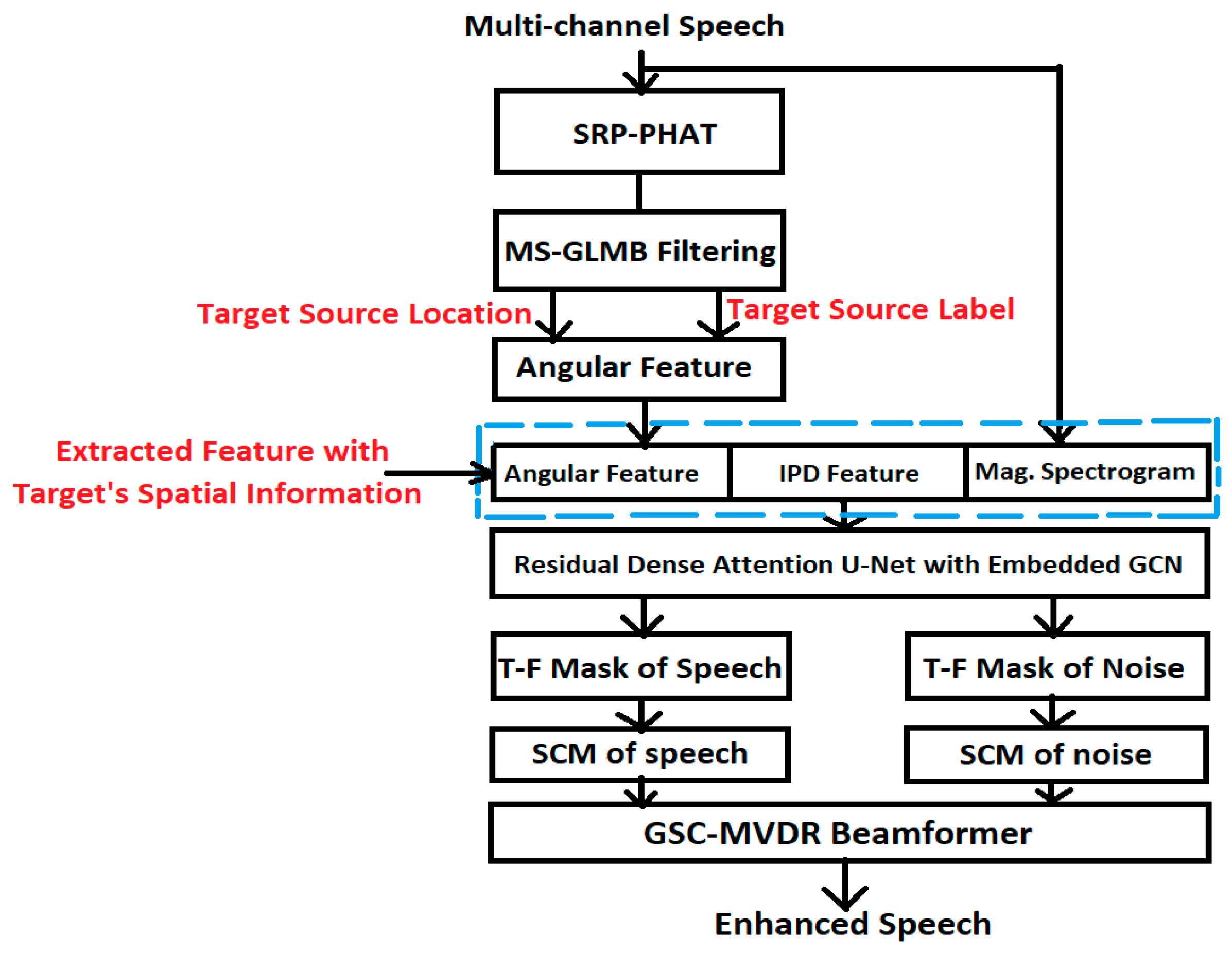
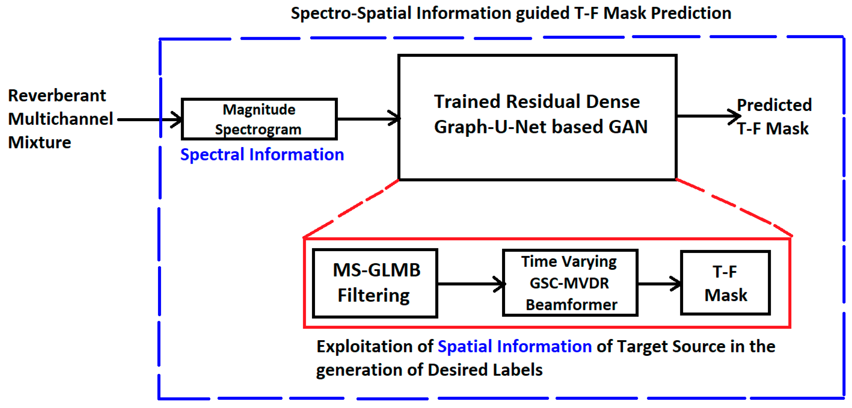
Construction of label-set data for training a neural architecture for target speech enhancement with the help of MS-GLMB filtering-based multi-source tracking and a time-varying MVDR beamformer, one which takes into account the effect of reverberation, noise and motion of the sources at each time frame. While the GLMB-assisted tracking relies on initial location information provided by steered response power phase transform (SRP-PHAT) [46], the inclusion of the tracking framework within the neural training procedure helps to develop the knowledge of spectro-spatial information of the moving sources within the neural architecture, so that it is able to generalize to “unseen” acoustic conditions as well and directly predict the desired T-F mask.

ii.

Construction of a residual dense convolutional U-Net architecture with an embedded GCRNN module, referred to as RD-graph-U-Net, which is applied in a GAN setting to predict the target source-specific mask.

The proposed approach is tested on publicly available datasets [47,48,49,50,51] using speech quality evaluation metrics [52,53,54]. The image source method (ISM) [55] is used to generate the room impulse response (RIR) between the source speaker and receiver microphone array. Adaptive momentum estimation (ADAM) [56] is selected as the optimization strategy to train the proposed neural architecture. Based on computer simulation results, it can be inferred that the proposed methodology improves the intelligibility of the speech corresponding to target source in motion, under noisy reverberant conditions involving multiple moving speech sources. The proposed approach is also tested with recorded RIRs obtained from Aachen impulse response (AIR) [57] database, where it shows good results. This is largely because of the signal discriminative capability of the proposed neural approach, which it acquires due to the training procedure outlined in Section 3. The proposed approach can be applicable in many practical scenarios such as conferencing [58], assistive listening devices [59] and speech transcription systems [60]. The remainder of the article is arranged as follows. Section 2 describes the system model of the overall methodology; Section 3 describes the proposed neural architecture-based speech enhancement module; Section 4 provides a brief discussion about the proposed approach; Section 5 presents some future research directions in this area; and, finally, Section 6 concludes this article.

2. System Model

Similar to magnitude–domain spectra, which are widely used in mono-aural speech enhancement, both real and imaginary spectrograms exhibit a spectro-temporal structure, which is useful for training the deep neural algorithm. While the complex spectrograms provide spectral cues, the spatial cues are obtained from the directional feature as well as inter-microphone phase difference (IPD). The combination of spectral and spatial cues can be referred to as spectro-spatial features, and it enables the neural beamformer to learn to suppress the interfering signals arriving from directions other than the target speech signal. In this section, the overall procedure of MS-GLMB filtering-assisted spectro-spatial feature construction is described, followed by the minimum variance distortionless response (MVDR) beamforming. While Section 2.1, Section 2.2 and Section 2.3 highlight the operations of SRP-PHAT for the localization of sources, MS-GLMB filtering for tracking of sources and exploitation of spectro-spatial information for guiding the T-F masking-based speech enhancement, the operation of the beamformer is described in Section 2.4. The beamformer selected for this work is GSC-MVDR of a time-varying nature, which exploits the spatial information of the sources and dynamically enhances the speech signal corresponding to the target source.

2.1. Steered Response Power Phase Transform (SRP-PHAT)

The SRP method, $P_{SRP}\left(\mathit{X}\right)$, can be treated as the output power of a filter-and-sum (F-S) beamformer, one which is steered to a set of source positions defined under a spatial grid. $\mathit{X}={[x,y]}^T$ is a vector, and represents the (x, y) position coordinates of the target acoustic source [46].

The phase transform (PHAT) is a weighting technique whose inclusion in the formulation of SRP helps to emphasize the phase information of the involved signals, thereby avoiding peak spreading [46]. For a microphone array with N elements, $P_{SRP}\left(\mathit{X}\right)$ can be expressed as the summation of individual generalized cross correlation (GCC) functions, $R_{nm}^{GCC}\left(\tau \right(\mathit{X}\left)\right)$:

$$P_{SRP}\left(\mathit{X}\right)={\sum }_{n=0}^{N-1}{\sum }_{m=0}^{N-1}{R}_{nm}^{GCC}\left(\tau \right(\mathit{X}\left)\right)$$

(1)

Unlike simplified scenarios, in realistic acoustic propagation environments, the signals received from different microphone elements do not simply differ from each other because of the delay that is dependent on the relative position of the source with respect to other microphone elements. This is due to the impairments caused by multipath effects like reverberation as well as the presence of ambient and diffuse noise. Hence, the mapping from SRP-PHAT to 3D positional coordinates using simple regression methods suffers from inaccuracies.

2.2. MS-GLMB Filtering

Multi-sensor (MS) RFS filtering-based tracking provides superior performance than single sensor tracking when multiple acoustic sources are in motion [6,31,32]. MS-GLMB filtering is applied in this work, whereby the propagation of the filtering density is achieved through a recursive procedure comprising two steps, namely the time update and the data update. In this work, the time-updated and data-updated filtering densities can be expressed in closed-form via the GLMB density [6,31,32]:

$$\pi ({\mathit{X}}_k)=∆({\mathit{X}}_k){\sum }_{{\theta }_{1:k}\in {\mathit{ϴ}}_{1:k}}{\omega }^{\left({\theta }_{1:k}\right)}\left(\mathcal{L}\left({\mathit{X}}_k\right)\right){\prod }_{{\mathit{x}}_k\in {\mathit{X}}_k}{p}^{\left({\theta }_{1:k}\right)}({\mathit{x}}_k)$$

(2)

In (2), ${\theta }_{1:k}\in {\mathit{ϴ}}_{1:k}$ represents the history of multi-array association mappings up to frame ‘k’, i.e., ${\theta }_{1:k}\stackrel{\wedge}{=}({\theta }_1,{\theta }_2\dots {\theta }_k)$. The term $\mathcal{L}\left({\mathit{X}}_k\right)$ can be further expressed as follows:

$$\mathcal{L}\left({\mathit{X}}_k\right)\stackrel{\wedge}{=}\{l:(x_k,l)\in {\mathit{X}}_k\}$$

(3)

Furthermore, in (2), the term $∆(.)$ denotes a distinct label indicator where $∆\left({\mathit{X}}_k\right)=1$ if and only if the cardinality of the label set denoted by $\left|\mathcal{L}\left({\mathit{X}}_k\right)\right|$ equals the cardinality of ${\mathit{X}}_k$ denoted by $\left|{\mathit{X}}_k\right|$. Each weight term ${\omega }^{\left({\theta }_{1:k}\right)}\left(\mathcal{L}\left({\mathit{X}}_k\right)\right)$ in (2) is a non-negative weight, such that their sum equals 1:

$${\sum }_{L\subseteq {Ỻ}_{0:k}}{\sum }_{{\theta }_{1:k}\in {\mathit{ϴ}}_{1:k}}{\omega }^{\left({\theta }_{1:k}\right)}\left(L\right)=1$$

(4)

Each of the non-negative weights in (3) and (4), represented by ${\omega }^{\left({\theta }_{1:k}\right)}\left(\mathcal{L}\left({\mathit{X}}_k\right)\right)$, can be interpreted as a probability of the sources with label set $\mathcal{L}\left({\mathit{X}}_k\right)$ being active, while at the same time being associated with the detections indicated by the history of multi-array association mappings up to the frame ‘k’, denoted by ${\theta }_{1:k}$. Finally, the term $p^{\left({\theta }_{1:k}\right)}\left({\mathit{x}}_k\right)$ in (2) represents the probability density of the source (with label ‘l’) that is located at the state $x_k=({\alpha }_k^{pos},{\alpha }_k^{vel})$. A detailed explanation of the terms in (2) can be found in [6,31,32]. The estimated position and label corresponding to the sources at each frame ‘k’ can be expressed as follows:

$$X_k^{est}=\{\left({\alpha }_{k,1,est}^{pos},l_1^{est}\right),\left({\alpha }_{k,2,est}^{pos},l_2^{est}\right)\dots ({\alpha }_{k,N_k,est}^{pos},l_{N_k}^{est}\left)\right\}$$

(5)

In (5), the term $N_k=\left|X_k^{est}\right|$ denotes the estimated number of sources at the kth frame. The estimated position and its corresponding label $\left({\alpha }_{k,i,est}^{pos},l_i^{est}\right),i=\mathrm{1,2}\dots N_k$ can be used to construct the steering vector corresponding to the direction of the target source represented by the position–label pair (${\alpha }_{k,d,est}^{pos},l_d^{est}$) while directing spectral nulls in the directions of the interfering sources denoted by the position–label pairs, $\left({\alpha }_{k,i,est}^{pos},l_i^{est}\right),\forall i\ne d$. As reported in [6], such a beamformer can dynamically enhance the speech corresponding to the target acoustic source by utilizing the estimates from the GLMB filter. In this work, we focus on utilizing MS-GLMB filtering to assist the construction of the target label set (in this case, the T-F mask specific to the target speech source) for the neural architecture. Due to the association of a unique label with every speech source within the environment, the MS-GLMB filtering helps to correctly discriminate between the target source and the interfering sources, which helps to train the subsequent deep neural architecture with an appropriately constructed label set specifically to the target source in motion under noisy reverberant conditions. The following sub-section provides more details on the role of MS-GLMB filtering in the overall target speech enhancement procedure.

2.3. Spectro-Spatial Information-Guided T-F Domain Masking for GSC-MVDR Beamformer

In prior state-of-the-art research works on neural network-assisted target speech enhancement [11,12,13], the angular feature (AF) was computed and used to construct an input feature set for the subsequent DL architecture, which predicts the target label (e.g., a mask specific to the target source). While the works outlined in [11,12,13] use AF as input feature for transformer- and recurrent neural network (RNN)-based deep neural architectures, the work outlined in [26] applies the feature set constructed using AF to a fully convolutional neural architecture arranged in a U-Net structure. The input feature set in all of these works comprised a concatenation of magnitude spectrogram, IPD, and AF. In addition, the works in [6,31,32] involve MS-GLMB filtering to compute the labels distinguishing the target source from the interfering sources at every time frame, which were also instrumental in constructing T-V beamformer weights. The overall procedure outlined in [26] is expressed in Figure 1, for reference.

Within the indoor environment, the area of potential target locations is divided into multiple angular sectors, each of which corresponds to an angular position of the target source at any time frame. The labelled RFS framework is helpful to demarcate the potential locations of the target speech source at different time frames from those of the interfering sources. This, in turn, helps to generate the training input dataset for the DL architecture, where the generated dataset reflects the effect of reverberation as well as the activity status of the target source. As the target and the interferers can be in different states of motion at different time frames, the dataset generated using the labelled RFS framework will reflect the state of the sources at different instants of time, which in turn helps to train the DL architecture more efficiently to predict the mask in a dynamic manner. The overall procedure can also be referred to as a form of beam zooming [20], where the applied DL architecture facilitates beam zooming on the potential location of the target source at each time frame.

In this work, the angular location information of the target source is utilized to create the training dataset on which the proposed neural architecture is trained. The dataset is constructed from the magnitude spectrogram, while the label set (T-F mask specific to target source) to train the neural architecture is constructed from the spatial information of the target source estimated by the MS-GLMB filter. The procedure is depicted in Figure 2.

While the AF used in previous works [11,12,13] is instrumental in achieving good target speech enhancement performance due to the construction of a feature set comprising spectro-spatial features corresponding to the target source, it may be helpful to use a simpler feature set (such as magnitude spectrogram) as input to the deep neural architecture, while still leveraging the spatial information of the moving target source at each frame to construct a suitable target label set to train the neural architecture. Hence, in this work, the proposed deep neural architecture is trained on the magnitude spectrograms of the received multi-channel reverberant mixture with the target source-specific T-F masks generated as labels, the latter having been generated by utilizing the spatial information of the multiple sources in motion. While direct estimation of a T-F mask from the complex spectra of received multichannel speech, as reported in [14,15], can also lead to dereverberation, speaker separation and noise cancellation, the exploitation of speaker-dependent spatial features for the generation of a label set for the deep neural architecture can lead to improvement in signal selectivity, which in turn can improve the performance of the beamformer.

Figure 3 shows the operation of the proposed neural framework during testing phase. The sequence of blocks at the lower half of this figure illustrates the implicit dependence of the neural processing on the spatial information of the target source. As the spatial information corresponding to the target source is utilized in the training of the proposed neural framework, the trained neural model incorporates the spatial information in addition to the spectral information. As such, the overall neural speech enhancement can be described as a spectro-spatial information processing framework. Hence, this methodology can also be referred to as spectro-spatial neural speech enhancement. Beamforming leads to an improvement in the SNR of the source-of-interest (SOI), resulting in a subsequent improvement in intelligibility under noisy and reverberant conditions. With the inclusion of T-F masking, a further improvement in the intelligibility of the SOI is achievable even in the presence of multiple interfering speakers. The training label generation procedure can be compactly explained in terms of subsections A and B.

2.4. TV-GSC-MVDR Beamformer

In this sub-section, the TV-MVDR beamformer based on a GSC structure, referred to as TV-GSC-MVDR, is described, and is utilized in the T-F mask generation process as part of the neural network training.

The MVDR beamformer can be formulated by the following constrained optimization problem:

$${min}_{\mathit{w}}{\mathit{w}}^H{\mathit{R}}_{\mathit{n}}\mathit{w} s.t.{\mathit{w}}^H.{\mathit{d}}_{steer}=1$$

(6)

The optimal solution to (6) is given as follows:

$${\mathit{w}}_{opt}={\displaystyle \frac{{\left({\mathit{R}}_{\mathit{n}}\right)}^{-1}.{\mathit{d}}_{steer}}{{{(\mathit{d}}_{steer})}^H{\left({\mathit{R}}_{\mathit{n}}\right)}^{-1}.{\mathit{d}}_{steer}}}$$

(7)

In Equations (6) and (7), the term ${\mathit{d}}_{steer}$ denotes the beam-steering vector which is computed from the TDOA (alternatively, DOA). The term ${\mathit{R}}_{\mathit{n}}$ denotes the noise covariance matrix, while the terms $\mathit{w}$ and ${\mathit{w}}_{opt}$ refer to MVDR beamformer weights and optimal MVDR beamformer weights, respectively. The selection of the steering vector for the kth frame (denoted by ${\mathit{d}}_k$) is achieved by exploiting the source state and corresponding label predicted by the MS-GLMB filter. As pointed out in [6], the steering vector can be selected by choosing the column vector from the steering matrix $D_{k,{\mathit{x}}_k^{est}}^{\left(q\right)}\left(f\right)$ for the kth time frame, where $D_{k,{\mathit{x}}_k^{est}}^{\left(q\right)}\left(f\right)$ can be expressed as follows:

$$D_{k,{\mathit{x}}_k^{est}}^{\left(q\right)}\left(f\right)=\left[\begin{array}{ccc}{e}^{j{\omega }_f(\tau ({\alpha }_{k,1}^{pos},u^{(q,1)}))}& \cdots & e^{j{\omega }_f(\tau ({\alpha }_{k,N_k^{est}}^{pos},u^{(q,1)}))}\\ ⋮& \ddots & ⋮\\ e^{j{\omega }_f(\tau ({\alpha }_{k,1}^{pos},u^{(q,M_q)}))}& \cdots & e^{j{\omega }_f(\tau ({\alpha }_{k,N_k^{est}}^{pos},u^{(q,M_q)}))}\end{array}\right]$$

(8)

In (8), the terms ${\alpha }_{k,1}^{pos}\dots {\alpha }_{k,N_k^{est}}^{pos}$ denote the positions of sources indexed 1…$N_k^{est}$ at frame ‘k’, $u^{(q,1)}\dots u^{(q,M_q)}$ denote the positions of microphones indexed $\left(q,1\right)\dots (q,M_q)$ for the qth array and microphone elements $(1\dots M_q)$, respectively. The term $\tau \left({\alpha }_{k,\mathrm{n}}^{pos},u^{\left(q,\mathrm{m}\right)}\right),\mathrm{n}=1\dots N_k^{est},m=1\dots M_q$ represents the time delay between nth source located at position ${\alpha }_{k,\mathrm{n}}^{pos}$ and the mth microphone element of the qth array represented by the position $u^{\left(q,\mathrm{m}\right)}$. The term ${\omega }_f$ denotes the angular frequency. Finally, the term $N_k^{est}$ denotes the estimated number of sources in the acoustic environment.

The steering vector selection is achieved by the following operation:

$$d_{k,l_i^{est}}^{\left(q\right)}\left(f\right){=\left({\left(D_{k,{\mathit{x}}_k^{est}}^{\left(q\right)}\left(f\right)\right)}^H\right)}^{\#}.r_{N_k^{est}}\left(l_i^{est}\right)$$

(9)

In (9), as described in [8], the term $r_{N_k^{est}}\left(l_i^{est}\right)$ denotes the selection operator, which selects the steering vector for the target speaker. The dimension of $r_{N_k^{est}}\left(l_i^{est}\right)$ depends on the number of estimated sources. The term $d_{k,l_i^{est}}^{\left(q\right)}\left(f\right)$ denotes the steering vector selected by the operation in (9) for the T-F point (k, f), where the suffix $l_i^{est}$ denotes the label of the source estimated by the MS-GLMB filtering algorithm, which helps to demarcate the target source from the interfering sources within the time frame. Thus, the dynamic MVDR beamformer weight for the kth frame can be expressed as follows:

$${{\mathit{w}}_{k,l_i^{est}}}^{\left(q\right)}={\displaystyle \frac{{{\mathit{R}}_n}^{-1}{.\mathit{d}}_{k,l_i^{est}}^{\left(q\right)}(f)}{{({\mathit{d}}_{k,l_i^{est}}^{\left(q\right)}\left(f\right))}^H.{{\mathit{R}}_n}^{-1}.{\mathit{d}}_{k,l_i^{est}}^{\left(q\right)}(f)}}$$

(10)

A. 

T-F Mask Generation for constructing label set for training neural architecture.

The beamformer output is utilized to compute the T-F mask corresponding to the target source at each time frame, which can lead to dynamic speech enhancement. Let the output of the beamformer at the T-F point (f, k) be denoted by $s_{k,l_i^{est}}^{MVDR}(f)$. As pointed out in [7], while the beamforming gain for the location of the target source might be higher than for the locations of interferers, the power spectrum in each T-F window may be dominated by interfering sources, in addition to noise and reverberation, during periods of inactivity of the target source or loud speech from the interfering sources. A spectral power ratio is computed to determine the T-F locations, which are dominated by the target speech and interference, respectively. This spectral power ratio can be expressed as follows:

$$G_{k,l_i^{est}}^{MVDR}\left(f\right)={\displaystyle \frac{{\left|s_{k,l_i^{est}}^{MVDR}\right(f\left)\right|}^2}{{\left|s_{k,l_j^{est}}^{MVDR}\left(f\right)\right|}^2}},i\ne j$$

(11)

In (11), while the numerator represents the power of the target signal (also referred to as SOI) in the spectral domain, the denominator also represents the power of the interferer source, $s_{k,l_j^{est}}^{MVDR}\left(f\right)$, identified by the estimated label $l_j^{est}$, in the spectral domain. The binary mask can be selected as:

$${\mathcal{M}}_{k,l_i^{est}}\left(f\right)=\left\{\begin{array}{c}1,if{G}_{k,l_i^{est}}^{MVDR}\left(f\right)\ge 1\\ 0,if{G}_{k,l_i^{est}}^{MVDR}\left(f\right)<1\end{array}\right.$$

(12)

Using the mask in (12), the enhanced speech corresponding to the target source can be obtained as follows:

$$S_{k,l_i^{est}}^{TF}\left(f\right)={\mathcal{M}}_{k,l_i^{est}}\left(f\right).s_{k,l_j^{est}}^{MVDR}\left(f\right)$$

(13)

By masking out those T-F bins, where the SOI is overwhelmed by speech from interfering sources as well as background noise, the intelligibility of the SOI can be considerably improved. The binary masks ${\mathcal{M}}_{k,l_i^{est}}\left(f\right)$ are generated from the label set for training the proposed residual dense Graph-U-Net-based GAN, as pictorially depicted in Figure 2 and Figure 3.

B. 

Dataset Construction

The steps involved in the construction of the dataset for training the neural architecture are mentioned in this subsection, as follows:

(i)

Selection of clean speech signals corresponding to three speakers from publicly available speech databases such as LibriSpeech and WSJ0mix. This is also mentioned in Section 4 on experimental results.

(ii)

Generation of acoustic room impulse responses (RIRs) using the image source method (ISM).

(iii)

Selection of reverberation times—RT60 of 550 ms, 250 ms and 50 ms—in three rooms of different dimensions.

(iv)

Generation of noise samples at different acoustic SNRs.

(v)

Creation of reverberant, noisy mixture of speech signals by convolution of clean speech signals with generated RIRs, with the addition of reverberation and noise samples.

(vi)

Estimation of position coordinates and label of each source using MS-GLMB filtering algorithm.

(vii)

Enhanced speech signal corresponding to target source across different time frames using GSC-MVDR beamforming.

(viii)

Construction of T-F mask from the output of beamformer as explained in Section 2.4 A.

(ix)

Creation of training dataset (to train the neural architecture) comprising the reverberant speech mixtures as input data and T-F masks as corresponding labels. In addition, the dataset is split into training, validation and testing datasets. This is further elaborated in quantitative terms in Section 4, where the experimental setup is described.

3. Residual Dense Convolutional Graph-U-Net-Based GAN for Target Speech Enhancement

Before discussing the overall neural architecture with the embedded graph convolutional network (GCN) module, the following subsections will present preliminaries on graph signal processing (GSP) [37] concepts and GAN operations [35,36].

3.1. Graph Signal Processing: Basic Concepts

Graph neural networks (GNNs) comprise a new class of neural architecture, which operates on graph-structured data. GNNs are capable of aggregating information from neighboring nodes of the graph, which help these neural architectures to encode structural–relational information into the overall representation. Consider 𝓖 as a graph where the set of nodes is represented by 𝓥 and the set of edges is represented by 𝓔. Mathematically, this can be expressed as follows:

$$\mathcal{G}=(\mathcal{V},\mathcal{E})$$

(14)

The GCN applies a non-linear transformation on the input $\mathcal{X}\in {\mathbb{R}}^{\left|\mathcal{V}\right|\times N}$, where $\left|\mathcal{V}\right|$ denotes the cardinality of the nodes of the graph and $N$ denotes the node feature size. The operation of the GCN can be mathematically represented as follows:

$${\mathcal{H}}^{\left(l\right)}=g({\mathcal{D}}^{-{\displaystyle \frac{1}{2}}}\mathcal{A}{\mathcal{D}}^{-{\displaystyle \frac{1}{2}}}{\mathcal{H}}^{(l-1)}{\mathcal{W}}^{(l-1)})$$

(15)

where $\mathcal{D}\in {\mathbb{R}}^{\left|\mathcal{V}\right|\times \left|\mathcal{V}\right|}$ is a diagonal matrix, $\mathcal{A}\in {\mathbb{R}}^{\left|\mathcal{V}\right|\times \left|\mathcal{V}\right|}$ is the adjacency matrix, ${\mathcal{H}}^{\left(l\right)}\in {\mathbb{R}}^{\left|\mathcal{V}\right|\times K}$ is the lth hidden layer with K hidden features, ${\mathcal{W}}^{(l-1)}$ is the set of trainable parameters at the (l-1)-th layer and $g(.)$ denotes the non-linear activation function. The term ${\mathcal{H}}^{\left(0\right)}$ represents the input $\mathcal{X}$ to the GCN.

3.2. Generative Adversarial Network: Basic Concepts

GAN was proposed by Goodfellow et al. in 2014 [35]. Its ability to generate realistic images and generalize well to pixel-wise, complex distributions has led to its widespread use in numerous applications in image restoration, computer vision, speech processing, wireless communications, etc. In speech enhancement, GAN architecture is capable of providing fast enhancement performance due to the absence of any recursive operation like RNN. Moreover, GAN architecture is able to learn from different speakers and noise types, which renders it capable of providing good target speech enhancement performance under noisy conditions. A GAN includes two models, the generator (G) and the discriminator (D). The generator (G)’s main task is to learn an effective mapping, which can imitate the real data distribution to generate novel samples related to those of the training set. This is achieved by G when it solely maps the data distribution characteristics to the manifold defined in the prior distribution, without memorizing input–output pairs. The GAN operates through an adversarial process which can be formulated as a mini–max game between G and D. The objective function of the mini–max game can be expressed as follows:

$${min}_G{max}_{D}V\left(D,G\right)=E_{x~p_{data}}\left[\log \left(D\left(x\right)\right)\right]+E_{z~p_z\left(z\right)}[\mathrm{l}\mathrm{o}\mathrm{g}(1-D\left(G\right(z\left)\right)\left)\right]$$

(16)

Several GAN architectures have been applied to target speech enhancement [21,22,23,24,25], where most of these are based on the conditional GAN (c-GAN) approach [24]. While traditional GAN can generate realistic samples, there is no control on the data being generated in such as an unconditional generative architecture. For speech enhancement tasks, it is necessary to control the generated data samples based on the noisy input samples (for e.g., received multi-channel speech mixture). This issue is addressed by the c-GAN framework, where the neural architecture is conditioned to control the data generation process based on the input data. c-GANs have demonstrated promising performance in noise suppression. The c-GAN architecture is trained to generate the spectrogram of clean speech given the noisy speech spectrogram; however, it ignores the phase mismatch problem.

3.3. Architecture of Residual Dense-U-Net with Embedded GCRNN

In prior research works involving graph convolutional blocks embedded in U-Net’s bottleneck layer [27,28,29], residual dense blocks were not explicitly applied in encoder and decoder parts of the architecture. In this article, a residual dense-U-Net architecture with a GCRNN embedded within the bottleneck layer (i.e., the GCRNN acts as the core embedding layer) is used as the neural framework of choice, and processes the spectro-spatial features to predict the target source-specific T-F mask. In addition, the skip connections also include GCRNN blocks. As mentioned earlier, neural architecture is applied in a GAN setting. In the generator, the embedded GCRNN’s nodes are set equal to the number of channels that are also referred to as kernels of the last RDN layer in the encoder part of the U-Net architecture. The generator and discriminator network’s operations are based on mini–max principles.

The encoder is composed of a stack of residual, densely connected convolutional blocks, whereas the decoder is composed of a stack of residual, densely connected deconvolutional blocks. Each densely connected block is a stack of four convolutional layers, with dense connections between layers. The output of each densely connected block in the encoder is passed through a GCRNN block-based skip pathway and then concatenated with the features of the corresponding residual densely connected de-convolutional block in the decoder.

A residual dense block (RDB) is a set of neural architecture, which can not only obtain the state from the preceding RDB via a contiguous memory (CM) mechanism but can also fully utilize all of the layers via local dense connections [41,42,43]. It contains densely connected layers, local feature fusion (LFF) and local residual learning together to lead to the CM mechanism. While residual learning modules, as in Res-Net architecture, can lead to better generalization capability of the model, they lack the dense concatenation of previous convolutional outputs to successive feature maps. Due to the presence of dense connectivity, a dense convolutional network, such as DenseNet [44], is able to utilize information from all previous convolutional operations, which allows the gradients to flow through several paths and thus enables richer information to be combined for feature extraction in consecutive layers. While the combination of residual and dense modules has been proposed in contemporary research works, their application in the domain of target speech enhancement for sources in motion seems limited. In the following subsections, the operation of the residual dense Graph-U-Net in a GAN setting is explained.

3.3.1. Generator Network: Residual Dense Graph-U-Net

The generator is a U-Net structure whose encoder is responsible for extracting the local and structural features. It halves the size of the feature maps using the convolutional kernel (whose stride is 2) instead of using pooling mechanism. Each convolutional layer is sequentially followed by one rectified linear unit (ReLU) and one instance normalization (IN) layer, which leads to significant reduction in the computational load. The process increases the receptive field of the network, which in turn improves model robustness.

The skip connections in the U-Net bypass the intermediate compression stages and directly pass fine-grained information to the decoder. As their presence facilitates flow of gradients through deeper layers of the overall network architecture, the skip connections can lead to better training performance by the network.

The operations of the generator network can be expressed in terms of hierarchical feature extraction and down-sampling at the encoder, the transformation of the multi-channel latent space of signals to the graph domain by the GCRNN module (embedded in the bottleneck layer), which leads to exploitation of spatio-temporal as well as spectral information in a more flexible manner, and up-sampling at the decoder. The operations of the residual dense blocks at the encoder part can be expressed as follows:

$$F_d=H_{RDB}^d\left(F_{d-1}\right)=H_{RDB}^d\left(H_{RDB}^{d-1}(\dots (H_{RDB}^1\left(F_0\right)\left)\right)\right)$$

(17)

In Equation (17), the term $H_{RDB}^d(.)$ represents the composite operation of convolution and ReLU at the RDB. As pointed out in [42,43], the residual dense block implements a CM mechanism by passing the state of the preceding residual dense block to each layer of the current residual dense block. The operation of the c-th convolution layer within the d-th residual dense block can be expressed in terms of the concatenation of the feature maps provided by the $(d-1)$th residual dense block as well as the (c − 1) convolutional layers $\mathrm{1,2}\dots (c-1)$ belonging to the d-th residual dense block, which results in $(G_0+\left(c-1\right).G_0)$ feature maps. $G_0$ is the number of output feature maps, also referred to as growth rate. This is the dense connectivity, which helps to preserve the feed-forward nature. The overall operation can be expressed as follows:

$$F_d^c=ReLU\left(W_d^c\left[F_{d-1},F_d^1,F_d^2\dots F_d^{c-1}\right]\right)$$

(18)

In Equation (18), $W_d^c$ represents the weights of the c-th convolutional layer, whereas $F_d^c$ represents the output of the c-th convolution layer within the d-th residual dense block. The operation of the LFF component of the residual dense block can be expressed as follows:

$$H_d^{LF}=H_d^{LFF}\left(\left[F_{d-1},F_d^1\dots ,F_d^c,\dots F_d^C\right]\right)$$

(19)

In Equation (19), $H_d^{LFF}(.)$ represents the 1-by-1 convolutional operation in the d-th RDB. Finally, the output of the RDB can be expressed as the output of local residual learning operation, as follows:

$$F_d=F_{d-1}+F_d^{LF}$$

(20)

The RDB employed in this work is pictorially depicted in Figure 4.

The last RDB of the encoder produces representations of dimension H-by-T’-by-F’, where H denotes the number of filters in the last residual dense convolutional layer of the encoder. As shown in Figure 5, the representations obtained at the last residual dense convolutional layer of the encoder parts are used to construct a graph with H nodes.

A. 

Graph Construction

In this article, the graph neural architecture is presented based on a message passing neural network, which operates through two phases, namely the message passing phase and the read-out phase [34,39]. The operations of these two steps for graph construction are expressed in terms of feature aggregation and update. The k-nearest neighbors (k-NN) [34] aggregation is utilized for graph construction, whereby it is possible to acquire k-NN by computing the Euclidean feature distance matrix, $D\in {\mathbb{R}}^{TF\times TF}$, formulated as follows:

$$d_{mn}=\sqrt{{\sum }_{\mathsf{D}}{(v_m-v_n)}^2}$$

(21)

In (21), the term $d_{mn}\in \mathsf{D}$ denotes the distance from node $v_m$ to node $v_n$. A graph is constructed by applying k-NN to every node where the resultant graph is of shape $\mathsf{D}\times F\times T\times k$, for which $F\times T$ nodes with $\mathsf{D}$ features are linked by directed edges. More specifically, each node in the constructed graph points to an edge feature set of size $k$ which contains $k$ neighbor nodes. A self-loop is also represented by pointing a node to itself. The graph convolution operation can be represented as a sequence of aggregation and update operations which can be expressed as follows:

$${\mathcal{G}}^{\prime }=\mathcal{F}(\mathcal{G},\mathcal{W})$$

(22)

$$=Update(Aggregate\left(\mathcal{G},W_{agg}\right),W_{update})$$

(23)

In Equations (22) and (23), $\mathcal{G}$ denotes the input graph of a specific GCN layer, ${\mathcal{G}}^{\prime }$ denotes the output graph of a specific GCN layer, $W_{agg}$ denotes the learnable weights of the aggregation operator and $W_{update}$ denotes the learnable weights of the update operator. The operation described in Equations (22) and (23) can be further elaborated with the help of Equations (24)–(27). If the set of neighbor nodes of the i-th node $v_i$ is represented by $\mathcal{N}\left(v_i\right)$, the graph convolution operation represented by Equations (22) and (23) can be re-expressed as follows:

$$v_i^{\prime }=h(v_i,g\left(v_i,\mathcal{N}\left(v_i\right),W_{agg}\right),W_{update})$$

(24)

While in the graph convolutional layer, the aggregate operator can be either of the permutation-invariant operators, such as mean, sum, max, attention etc., the max-relative operator is applied in Equation (24) for the aggregate operation, which can be expressed by Equations (25) and (26), as follows:

$${\Psi }_{ji}=v_j-v_{i}s.t.v_j\in \mathcal{N}\left(v_i\right)$$

(25)

$$g\left(.\right)=v_i^{\prime }=[v_i,\max \left\{{\Psi }_{ji}\right\}]$$

(26)

The update operation in Equation (24) is implemented by a multi-layer perception (MLP), as follows:

$$h\left(.\right)=MLP\left(Concat\left(v_i,v_i^{\prime }\right)\right)$$

(27)

• B. Operation of the GCRNN module

The output of the last RDB, denoted by $F_d$ of dimensions H-by-T’-by-F’, is treated as a graph signal with H nodes and feature size T’*F’. The construction of the graph is mentioned in subsection A. The thus-constructed graph is processed by the GCRNN module embedded in the bottleneck layer, which acts as a bridge between the encoder and decoder. This bottleneck layer is responsible for capturing all of the critical features while maintaining spatial information. The output of the GCRNN layer is forwarded through the different residual dense convolutional layers of the decoder part, as a result of which the hidden features are transformed to the original dimension at the output of the decoder of the overall U-Net architecture. Each skip connection pathway connecting an encoder layer with the corresponding decoder layer in the U-Net architecture is also considered by a GCRNN block. In this work, the GCRNN is a GCN for feature extraction and is selected together with long short-term memory (LSTM) for sequence learning. The overall operations of the GCRNN module can be expressed as follows:

$$F_t^{GCN}={CNN}_{\mathcal{G}}\left(F_{d,t}\right)$$

(28)

$$i_t=\sigma (W_{xi}.F_t^{GCN}+W_{hi}.h_{t-1}+W_{ci}\odot c_{t-1}+b_i)$$

(29)

$$f_t=\sigma (W_{xf}.F_t^{GCN}+W_{hf}.h_{t-1}+W_{cf}\odot c_{t-1}+b_f)$$

(30)

$$c_t=f_t\odot c_{t-1}+i_t\odot \mathrm{t}\mathrm{a}\mathrm{n}\mathrm{h}(W_{xc}.F_t^{GCN}+W_{hc}.h_{t-1}+b_c)$$

(31)

$$o_t=\sigma (W_{xo}.F_t^{GCN}+W_{ho}.h_{t-1}+W_{co}\odot c_t+b_o)$$

(32)

$$h_t=o_t\odot \mathrm{t}\mathrm{a}\mathrm{n}\mathrm{h}\left(c_t\right)$$

(33)

In (28), the term $F_{d,t}$ represents the input to the GCN denoted by the expression ${CNN}_{\mathcal{G}}(.)$, whereas the term $F_t^{GCN}$ represents the output of the GCN gate. As evident from the above discussion, the input $F_{d,t}\in {\mathbb{R}}^{H\times T\prime .F\prime }$ is the output of the encoder with H nodes and T’*F’ features.

3.3.2. Discriminator Network

The discriminator is similar to the encoding stage of the generator network. Thus, it consists of a series of densely connected residual convolution blocks. Leaky ReLU (lReLU) is applied following the convolutional layers in the discriminator. After the down sampling process, the feature maps will pass through a fully connected layer whose output is a confidence value representing the similarity between the generated mask and true mask.

The functionalities of the generator and discriminator can be concisely expressed by the following steps:

Update discriminator such that (x, y)-pairs are classified as real i.e., $D\left(x,y\right)=1$.

Update discriminator such that the pair comprising generated samples $x_{pred}$ and true labels $y$ are classified as fake i.e., $D\left(x_{pred},y\right)=0$.

Freeze the discriminator and update the generator such that the discriminator classifies the $(x_{pred},y)$-pair as real i.e., $D\left(x_{pred},y\right)=1$.

3.3.3. Loss Function Used in Residual Dense Graph-U-Net GAN

For updating the generator and discriminator networks, the least-squares (LS) cost function is utilized in this work, and substitutes the conventional cross-entropy loss function of the binary classifier in the discriminator by an LS-based loss function. Furthermore, the application of the LS-based loss function can lead to improvements in the quality of the generated samples in the generator network and, due to increased stability, improvements in the training performance of the generator network. Moreover, an additional loss function term is also used in the GAN network, which minimizes the L1 distance between the generated samples and the clean samples. The L1 term is controlled by a hyper-parameter term, λ. The loss functions corresponding to the discriminator and generator networks are given by (28) and (29) respectively:

$$Discriminator:{min}_D\mathcal{L}\left(D\right)={\displaystyle \frac{1}{2}}{\mathbb{E}}_{\mathit{x},\mathit{y}~p_{data}(\mathit{x},\mathit{y})}{[D\left(\mathit{x},\mathit{y}\right)-1]}^2+{\displaystyle \frac{1}{2}}{\mathbb{E}}_{\mathit{z}~Z,\mathit{y}~p_{data}\left(\mathit{y}\right)}{\left[D\right({\mathit{x}}^{est},\mathit{y}\left)\right]}^2$$

(34)

$$Generator:{min}_G\mathcal{L}\left(G\right)={\mathbb{E}}_{\mathit{z}~Z,\mathit{y}~p_{data}\left(\mathit{y}\right)}{\left[D\right({\mathit{x}}^{est},\mathit{y})-1]}^2+\lambda .{\left|\right|{\mathit{x}}^{est}-\mathit{y}\left|\right|}_1$$

(35)

3.4. Loss Function

In most works on speech enhancement using DL, the mean square error (MSE)-based loss function is used as the criterion for training the neural architecture. In addition to MSE, the scale invariant signal-to-noise ratio (SI-SNR) can also be incorporated within the loss function as a training criterion. A loss function combining the SI-SNR and MSE for better training of the neural architecture has been applied in [27], leading to good speech enhancement performance under low SNR conditions. Following [27], we also apply the combination of SI-SNR and MSE as the loss function in this work, whereby the formulation of the loss function can be explained by (36)–(40), as follows:

$$x_{target}={\displaystyle \frac{<x_{enh},x_{clean}>.x_{clean}}{{\left|\left|x_{clean}\right|\right|}_2^2}}$$

(36)

$$z_{noise}=x_{enh}-x_{clean}$$

(37)

$${\mathcal{L}}_{SI-SNR}\left(x_{clean},x_{enh}\right)=10.{log}_{10}\left({\displaystyle \frac{\left|\right|{x_{target}\left|\right|}_2^2}{{\left|\right|z_{noise}\left|\right|}_2^2}}\right)$$

(38)

In (36)–(38), the terms $x_{enh}$ and $x_{clean}$ represent the enhanced and clean target speech signals in the time domain, respectively. The operation $<.,.>$ denotes the dot product operation between any two vectors. In (38), ${\left|\right|.\left|\right|}_2^2$ denotes the L2 (or Euclidean) norm. The SI-SNR-based loss function is denoted by ${\mathcal{L}}_{SI-SNR}(.)$. If the true mask and estimated mask are denoted by $M_{clean}$ and $M_{est}$ (where $M_{est}\in \{M_s^{DL},M_{int+noise}^{DL}\}$), respectively, then the MSE loss function can be expressed as follows:

$${\mathcal{L}}_{MSE}\left(M_{clean},M_{est}\right)={\sum }_{t,f}[{\left({Re(M}_{clean}\right)-Re\left(M_{est}\right))}^2+{\left({Im(M}_{clean}\right)-Im\left(M_{est}\right))}^2]$$

(39)

In (39), $Re(.)$ and $Im(.)$ denote the real and imaginary parts, respectively. Based on (38) and (39), the combined loss function can be expressed as follows:

$$\mathcal{L}\left(x_{clean},x_{enh}\right)={\mathcal{L}}_{SI-SNR}\left(x_{clean},x_{enh}\right)+\log \left({\mathcal{L}}_{MSE}\left(M_{clean},M_{est}\right)\right)$$

(40)

4. Computer Simulation Results

4.1. Experimental Dataset

4.1.1. Speech Source Parameters

In order to evaluate the effectiveness of the proposed methodology, in this work we have constructed a new dataset of simulated speech sources in motion under noisy, reverberant conditions. Speech signals corresponding to the sources have been selected from the WSJ0mix [46] and LibriSpeech [47] speech corpuses, while the noise samples were selected from CHiME-3 [48], the diverse environments multichannel acoustic noise database (DEMAND) [49] and environment sound classification (ESC-50) [50] databases.

The signals from WSJ0mix and CHiME-3 are randomly selected and mixed for SNRs between 2 dB and 10 dB. The selected noise samples from the DEMAND database correspond to noise signals recorded in diverse acoustic environments such as a busy subway station, an office cafeteria, and a university restaurant. Fifteen noises were selected for training and validation sets, whereas three noises were selected for the testing set. The SNR selected for training and validation sets were randomly sampled between −5 dB and 0 dB. However, for the testing set, different SNR values of −5 dB, 0 dB and 5 dB were used. ESC-50 is a dataset for environment sound samples, one which contains a total of 2000 environmental sound recordings organized into 5 primary classes, namely animal, natural, human, interior/domestic and exterior. The dataset is labelled with 50 classes and is also available with noise added to the audio signals. Therefore, the ESC-50 dataset also provides a plethora of sound waveforms which can be added to speech waveforms in the indoor environment to illustrate the target speech waveform enhancement task. In this work, a training set comprising 7000 speech mixtures was created for training the proposed neural architecture, whereas a validation set comprising 1000 speech mixture signals for validation and a testing set comprising 1000 speech signal mixtures for testing the proposed neural architecture were also created. MATLAB 2024b is used to generate the reverberant speech signals, whereas Tensorflow 2.11 is used with Python version 3.9 to train and test the proposed neural approach. The signals were sampled at 16 KHz. In addition, a Hamming window of a duration of 20 ms was utilized to segment the waveforms into a set of time frames, whereby an overlap of 50% between adjacent frames is applied. The size of the DFT applied to each time frame of received speech signal mixture is therefore of a length of 320 points.

The room impulse response (RIR) between the source speaker and the receiving microphone array is generated using the ISM [55] approach. The acoustic scene parameters used for this simulation are tabulated in

Table 1. Acoustic scene parameters.

Room Dimensions in x,y Coordinates (in m)	X (14 m)	Y (22 m)
SNR (in dB)	0–60 (training)	15, 35, 80 (testing)
Reverberation time, T60 (in ms)	50, 250, 550	550
Microphone array	Linear	6 sensors per array
Number of speakers	3 (training)	3 (testing)

. For each simulated RIR, the room geometry, array position and start and end coordinates of the source speakers are randomly selected. Similar parameters of acoustic scenes and microphone array configurations have also been considered in [6,26,31]. However, this work involves a DL-based combined approach of tracking and enhancement, and the DL parameters used in this work are mentioned in Section 4.3. The speech signals corresponding to the 3 speakers are simulated inside a room with the dimensions of 10 m by 18 m by 6 m, where the reverberation times denoted by RT60 are considered as 50 ms, 250 ms and 550 ms, respectively. During the training phase, RT60 values of 50 ms, 250 ms and 550 ms are chosen, whereas during the testing phase, RT60 values of 550 ms are chosen to test the performance of the DL architecture. A single microphone array with 6 sensors is simulated. The maximum number of speakers chosen is 3. The RIRs were generated using ISM [54] at the above-mentioned reverberation times. The sampling frequency is taken to be 16,000 Hz.

In the simulation setting, a maximum number of 3 speakers is selected, and these are placed in continuous motion inside the room. The different microphone sensors ‘coordinates are taken to be (7.11, 6.0), (7.11, 5.55), (7.11, 5.10), (7.11, 4.65), (7.11, 4.20) and (7.11, 3.75). The motion of the speakers is modelled by the Langevin model. Details about the Langevin model can be found in [6] and the references therein. The state equations governed by the Langevin model can be expressed as follows:

$${\alpha }_{k+1}^{pos}={\alpha }_k^{pos}+\varnothing .{\alpha }_k^{vel}$$

(41)

$${\alpha }_{k+1}^{vel}=e^{-\beta \varnothing }.{\alpha }_k^{vel}+\vartheta .\sqrt{1-e^{-2\beta \varnothing }}.{\Sigma }_k$$

(42)

In (41) and (42), ${\alpha }_k^{pos}$ and ${\alpha }_k^{vel}$ represent the 3D position vector and velocity vector of the target speaker in motion. The terms β, ϕ and ${\Sigma }_k$ represent the rate constant which controls the rate of decay of velocity, discretization time step interval, and process noise, respectively. The process noise ${\Sigma }_k$ is a 3D Gaussian vector with mean zero and covariance, ${\sigma }_{\Sigma }.{\sigma }_{\Sigma }^T$, where ${\sigma }_{\Sigma }$ represents the standard deviation of the process noise. The Langevin model parameters used for the simulation are included in

Table 2. Parameters of the Langevin model.

Parameters	Values
$\mathit{\beta }$ (in s−1)	10
$\mathit{\vartheta }$ (in ms−1)	1
$\mathit{\varphi }$ (in ms)	32
${\mathit{\sigma }}_{\mathit{\Sigma }}$ (in ms−1)	${[4.5,4.5,4.5]}^T$

.

4.1.2. MS-GLMB Filtering Parameters

The 3D coordinates of the target source are obtained from the SRP-PHAT data. These 3D coordinates are used to construct the measurement set for the MS-GLMB filter.

Table 3. Parameters of the MS-GLMB filter.

${\mathit{r}}_{\mathit{B}}\left({\mathit{l}}_1\right)$	0.005
${\mathit{r}}_{\mathit{B}}\left({\mathit{l}}_2\right)$	0.005
${\mathit{r}}_{\mathit{B}}\left({\mathit{l}}_3\right)$	0.005
${\mathit{\mu }}_{\mathit{B}}^{\left(1\right)}$	${\left[5.01.01.8000\right]}^T$
${\mathit{\mu }}_{\mathit{B}}^{\left(2\right)}$	${\left[4.03.01.5000\right]}^T$
${\mathit{\mu }}_{\mathit{B}}^{\left(3\right)}$	${\left[2.50.51.5000\right]}^T$
${\mathit{P}}_{\mathit{B}}^{\left(1\right)}$	diag(${[0.15;0.15;0.15;0.15;0.15;0.15]}^T)$
${\mathit{P}}_{\mathit{B}}^{\left(2\right)}$	diag(${[0.15;0.15;0.15;0.15;0.15;0.15]}^T)$
${\mathit{P}}_{\mathit{B}}^{\left(3\right)}$	diag(${[0.15;0.15;0.15;0.15;0.15;0.15]}^T)$

outlines the parameters corresponding to the MS-GLMB filter. In this work, the same parameters of MS-GLMB filter are used as used in [6].

The birth parameters of the 3 speakers can be denoted by ${\left\{r_B\left(l_i\right),p_B(.,l_i)\stackrel{\wedge}{=}\mathcal{N}(.;{\mu }_B^{\left(i\right)},P_B^{\left(i\right)}\left.)\right\}\right.}_{i=1}^3$, where $r_B\left(l_i\right)$ denotes the birth probability of the ith speaker with label $l_i$ and $p_B(.,l_i)$ denotes the birth probability density of the ith speaker, which is a Gaussian with mean ${\mu }_B^{\left(i\right)}$ and covariance $P_B^{\left(i\right)}$. The Gaussian mean ${\mu }_B^{\left(i\right)}$ represents a vector which contains the expected location of the birth of the ith speaker with label $l_i$. The covariance $P_B^{\left(i\right)}$ signifies the spatial uncertainty associated with the ith speaker. The estimated label corresponding to the target speaker is obtained by MS-GLMB filtering. The label information is helpful in demarcating the trajectories corresponding to the different speech sources within the environment, which in turn helps the algorithm to track the sources in motion across all the time frames.

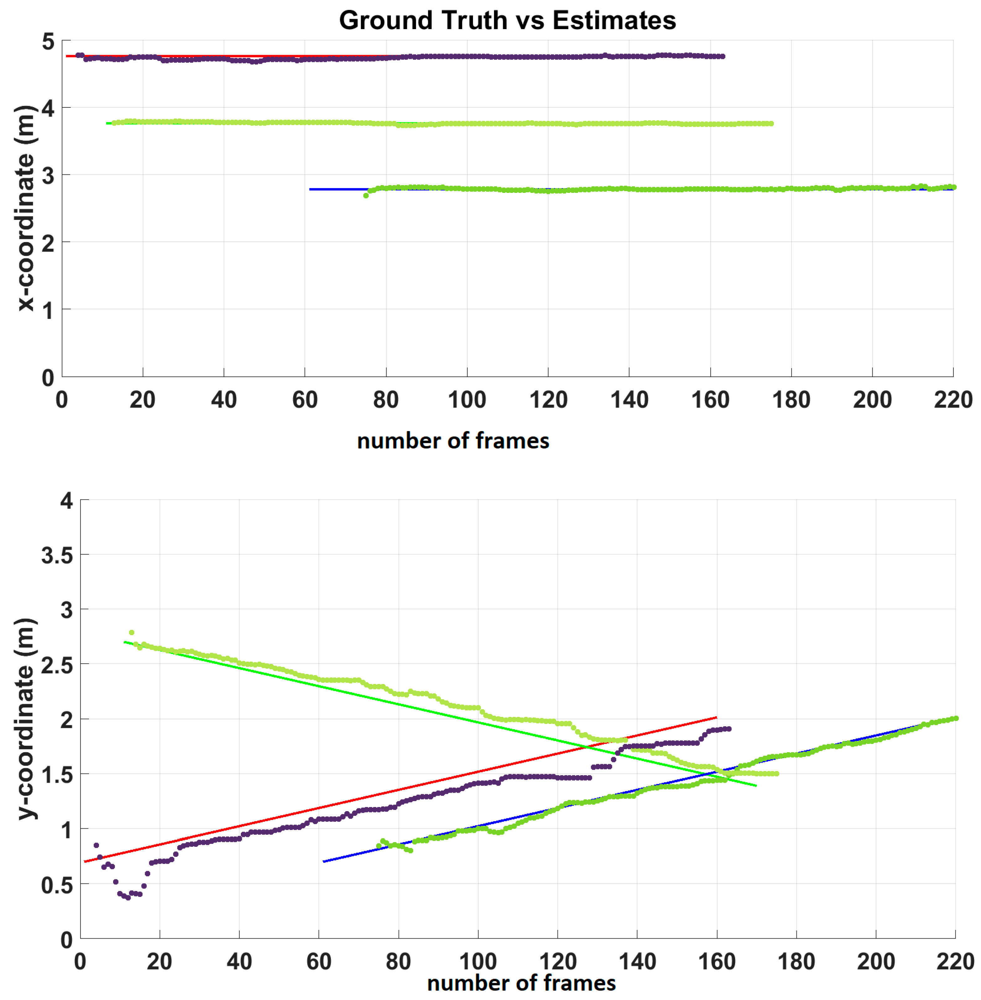
4.2. MS-GLMB Filtering Based Multi-Source Tracking Filter

As mentioned earlier, the multi-array measurements are processed by the MS-GLMB filter at each frame, whereby the source tracks comprising positions and labels are estimated. In this regard, it is useful to mention that a track can be considered as a function whose domain comprises the set of time instants at which the source exists. In general, a track corresponding to a particular source exists when the estimated positions of that source across the time frames can be associated with a common label. In practical scenarios, such as online multi-object tracking, the source may intermittently speak or disappear from the scene, giving rise to fragmented (or broken) tracks. Another scenario which frequently happens in online multi-object tracking is that which, when multiple sources are in very close proximity, the associated labels and their tracks may interchange. Figure 6 depicts the prediction of the (x-, y-) coordinates across all of the time frames by the MS-GLMB filtering at RT60 = 550 ms and compares against the ground truth positions.

As observed from Figure 6, the application of MS-GLMB filtering to multi-source tracking in the acoustic domain leads to estimation of source tracks, which can still closely resemble the ground-truth tracks under the effects of noise and reverberation. This is due to the ability of the MS-GLMB filter to resolve the space-time permutation problem by jointly estimating the source labels and positions. This framework can account for noise, false positives and false negatives in the multi-array measurements (in this case, SRP-PHAT-based acoustic measurement at each array). Furthermore, source motions, labels as well as their appearances and disappearances are also incorporated into the formulation of the MS-GLMB filter for multi-source tracking. Because of these advantages, the MS-GLMB filter can guide the construction of input features in order to train the proposed neural framework, whereby the input feature set includes the directional information of the target source provided by the MS-GLMB filter.

4.3. Experimental Setup for the Residual Dense Graph-U-Net

In order to evaluate the extent to which the proposed methodology works under different acoustic environments, the proposed approach is subject to different room environments where the room dimensions are different from those of the original environment. The room dimensions considered for evaluating the proposed approach under different acoustic conditions are chosen as 5.80 m by 3.30 m by 2.00 m, 7.50 m by 3.50 m by 2.80 m and 10.50 m by 6.50 m by 3.40 m. The rooms corresponding to these three different room dimensions are designated as ‘Test Room I’, ‘Test Room II’, and ‘Test Room III’, respectively.

Table 4. Summary of experimental conditions.

Configuration of Mask Estimation Network (Generator)
ENCODER
Number of down-sampling layers	5
Number of RDBs in each encoder layer	1
Kernels of CNN layers in each encoder block	{64, 128, 128, 128, 32}
Kernel sizes of CNN layers	3 × 3
Stride	2 × 2
Padding	0
DECODER
Number of up-sampling layers	5
Number of RDBs in each decoder layer	5
Kernels of CNN layers in each decoder block	{32, 128, 128, 128, 64}
Kernel sizes of CNN layers	3 × 3
Stride	2 × 2
Padding	0
Loss Function	MSE
Optimization criterion	ADAM
Learning rate	10−4
Batch size	32

presents the overall summary of experimental conditions, while

Table 5. Test room dimensions.

Test Room I	5.80 m by 3.30 m by 2.00 m
Test Room II	7.50 m by 3.50 m by 2.80 m
Test Room III	10.50 m by 6.50 m by 3.40 m

depicts the test rooms’ dimensions.

Table 6. Microphone positions for Test Room I, Test Room II and Test Room III.

Position 1	[(2.40, 0.3), (2.60, 0.3), (2.80, 0.3), (3.0, 0.3), (3.20, 0.3), (3.40, 0.3)]
Position 2	[(4.00, 0.3), (4.20, 0.3), (4.40, 0.3), (4.60, 0.3), (4.80, 0.3), (5.00, 0.3)]
Position 3	[(3.6, 3.11), (3.4, 3.11), (3.2, 3.11), (3.0, 3.11), (2.8, 3.11), (2.6, 3.11)]

presents the positions of microphone elements within each test room.

The reverberation time used for these environments is RT60 = 550 ms. The microphone sensors’ coordinates are varied so that the positions of the array elements are different from those placed in the room in which the algorithm was originally trained. The different positions of the microphone sensors in the array in the test environments are tabulated in Table 6. The configurations selected in Table 5 and Table 6 have also been applied in prior research works and are included in [31,45]. In particular, the research work presented in [45] utilized a Dense-U-Net architecture, which performs localization of acoustic sources in motion. The training procedure involved in that research work involved training and testing the Dense-U-Net architecture using three test rooms as well as a six-element linear microphone array whose positions were varied in the three rooms to effectively train the neural architecture to predict the locations of the sources with high accuracy in the presence of acoustic impairments like reverberation as well as sources’ motion. Motivated by the results presented in [45], the work presented in this article also utilizes the same test room dimensions and microphone array positions as in [45] for testing the proposed speech enhancement approach.

In the test environments, apart from varying the microphone sensors’ positions, the SNR is varied such that the selected acoustic SNRs fall in the set [0 dB, 10 dB, 20 dB, 30 dB, 40 dB, 50 dB, 60 dB]. To test the proposed approach, an SNR value is randomly selected from the above set of SNRs, whereby the test room dimensions and positions of the microphone array sensors are also randomly selected from Table 5 and Table 6 respectively.

4.4. Evaluation Metrics

The proposed methodology is compared with other methodologies which have also been applied to the moving speech sources scenario. As evaluation metrics, enhanced short-time objective intelligibility (ESTOI) [51], perceptual evaluation of speech quality (PESQ) [52], SI-SNR [18] and signal-to-distortion ratio (SDR) [53] are used for performance comparison in this work. In this section, the spectrograms of the clean target speech, reverberant mixture and enhanced speech are first presented for comparison. Second, the proposed approach is evaluated against other state-of-the-art neural speech enhancement approaches in terms of some established evaluation metrics. Figure 7a–c depict the spectrograms of clean target, reverberant mixture, and enhanced speech corresponding to waveforms selected from the LibriSpeech dataset.

Figure 8a–c depict the spectrograms of the clean target, reverberant mixture, and enhanced speech corresponding to the waveforms selected from the Ws2J0mix dataset.

As evident from the spectrograms presented in Figure 7 and Figure 8, the proposed neural approach of speech enhancement successfully cancels the background noise and reverberation to enhance the target speech, even when the sources are in motion and intermittently speaking. This is evident from Figure 7c and Figure 8c. Next,

Table 7. Performance comparison of different state-of-the-art approaches for speech dereverberation under dynamic conditions at 3 different reverberation times.

Method	RT60 = 550 ms		RT60 = 250 ms		RT60 = 50 ms
	PESQ	SI-SNR (dB)	PESQ	SI-SNR (dB)	PESQ	SI-SNR (dB)
MS-GLMB filter-assisted DS	2.41	4.42	2.79	10.73	2.91	13.94
TI-MVDR	2.43	2.35	2.73	4.42	2.76	5.13
Online-MVDR	3.22	4.85	3.38	5.62	3.45	6.52
MS-GLMB filter-assisted MVDR	3.28	5.65	3.44	6.55	3.51	7.66
DOA-MVDR	3.43	8.85	3.49	9.75	3.55	10.36
Mask-MVDR with self-attention	3.57	10.37	3.60	10.55	3.65	12.66
U-Net with embedded GCN	3.56	10.54	3.65	11.66	3.67	12.78
RD-GAN	3.58	10.58	3.67	11.72	3.69	12.82
RD-Graph-U-Net-GAN (proposed approach)	3.60	10.77	3.70	11.88	3.85	12.86

shows a performance comparison in terms of objective metrics such as PESQ and SI-SNR between the proposed approach and other state-of-the-art approaches at three different RT60 values (550 ms, 250 ms and 50 ms), which tackle the problem of speech enhancement including speech dereverberation and interference cancellation under dynamic scenarios.

4.4.1. Beamformer Baselines for Performance Comparison

In this section, an overview of the state-of-the-art beamformer approaches is presented. The proposed approach is compared with these approaches for target speech enhancement under reverberant conditions involving moving sources. The evaluated baseline beamformers can be denoted by time invariant MVDR (TI_MVDR), online MVDR (online_ MVDR) involving online computation of SCM, block MVDR (BLK_ MVDR) involving block-wise processing of time-varying SCM, direction-of-arrival (DOA)-based MVDR (DOA_MVDR) baseline, mask-based MVDR using attention mechanism (ATT_MASK_ MVDR), residual dense GAN-based beamformer (RD-GAN) [25] and GCN-based MVDR (GCN_ MVDR). Outlines of such beamformer baselines can be obtained from [8,25,29].

TI-MVDR Beamformer Baseline

The TI_MVDR system computes the SCM in a time-invariant fashion, where the assumption is that the transfer function is static within an utterance. The time-invariant SCMs can be computed as follows:

$${\mathit{\Phi }}_{\mathit{f}}^{\mathit{v}}={\sum }_{\mathit{\tau }=1}^{\mathit{T}}{\displaystyle \frac{1}{{\sum }_{{\mathit{\tau }}^{\prime }=1}^{\mathit{T}}{\mathit{m}}_{{\mathit{\tau }}^{\prime },\mathit{f}}^{\mathit{v}}}}{\mathit{m}}_{\mathit{\tau },\mathit{f}}^{\mathit{v}}.{\mathit{Y}}_{\mathit{\tau },\mathit{f}}.{\mathit{Y}}_{\mathit{\tau },\mathit{f}}^{\mathit{T}}$$

(43)

In (43), the term ${\mathit{Y}}_{\mathit{\tau },\mathit{f}}.{\mathit{Y}}_{\mathit{\tau },\mathit{f}}^{\mathit{T}}$ can be represented by ${\mathit{\Psi }}_{\mathit{\tau },\mathit{f}}^{\mathit{v}}$, which can be referred to as an instantaneous SCM (ISCM) at the T-F bin. The term ${\mathit{m}}_{{\mathit{\tau }}^{\prime },\mathit{f}}^{\mathit{v}}\in \left[0, 1\right]$ represents the T-F mask. In (43), the superscript $\mathit{v}\in \{\mathit{S},\mathit{N}\}$ denotes the indices of speech (S) and noise (N).

Online MVDR Beamformer Baseline

The online_MVDR system involves the application of a recursive approach to compute a time-varying (T-V) SCM, ${\mathit{\Phi }}_{\mathit{t},\mathit{f}}^{\mathit{v}}$. Such an approach can lead to the computation of SCMs for the MVDR beamformer in an online manner. The recursive computation of the online SCMs can be expressed as follows:

$${\mathit{\Phi }}_{\mathit{t},\mathit{f}}^{\mathit{v}}=\mathit{\alpha }.{\mathit{\Phi }}_{\mathit{t}-1,\mathit{f}}^{\mathit{v}}+{\mathit{\Psi }}_{\mathit{t},\mathit{f}}^{\mathit{v}}={\sum }_{\mathit{\tau }=1}^{\mathit{t}}{\mathit{\alpha }}^{\mathit{t}-\mathit{\tau }}.{\mathit{\Psi }}_{\mathit{\tau },\mathit{f}}^{\mathit{v}}$$

(44)

The online_MVDR approach enables the computation of SCMs as well as MVDR beamformer weights at each time frame, which in turn allows for the tracking of a speech source.

Block MVDR Beamformer Baseline

The BLK_MVDR system involves the computation of SCM corresponding to each time block of the signal into which it is divided. The block-wise computation of the time-varying SCMs can be expressed as follows:

$${\mathit{\Phi }}_{\mathit{t},\mathit{f}}^{\mathit{v}}={\sum }_{\mathit{\tau }=\mathit{t}-\mathit{L}}^{\mathit{t}+\mathit{L}}{\displaystyle \frac{1}{\sum _{{\mathit{\tau }}^{\prime }=\mathit{t}-\mathit{L}}^{\mathit{t}+\mathit{L}}{\mathit{m}}_{{\mathit{\tau }}^{\prime },\mathit{f}}^{\mathit{v}}}}.{\mathit{\Psi }}_{\mathit{\tau },\mathit{f}}^{\mathit{v}}$$

(45)

In (45), the term $\mathit{L}$ denotes the block-size parameter and $(2\mathit{L}+1)$ frames were utilized for the computation of SCM for each block.

DOA-Based MVDR Beamformer Baseline

The DOA_MVDR system computes the steering vector from the DOA information which can be expressed as follows:

$${\mathit{h}}_{\mathit{t},\mathit{f}}={[{\mathit{e}}^{\mathit{j}{\displaystyle \frac{2\mathit{\pi }\mathit{f}}{\mathit{\upsilon }}}{\mathit{\tau }}_1},{\mathit{e}}^{\mathit{j}{\displaystyle \frac{2\mathit{\pi }\mathit{f}}{\mathit{\upsilon }}}{\mathit{\tau }}_2}\dots {\mathit{e}}^{\mathit{j}{\displaystyle \frac{2\mathit{\pi }\mathit{f}}{\mathit{\upsilon }}}{\mathit{\tau }}_{\mathit{C}}}]}^{\mathit{T}}$$

(46)

In (46), ${\mathit{h}}_{\mathit{t},\mathit{f}}$ denotes the beam steering vector, υ the speed of sound waves, and ${\mathit{\tau }}_{\mathit{C}}$ the propagation delay w.r.t origin for microphone indexed $\mathit{C}$. The steering vector is constructed from the DOA information and can be used to construct SCM corresponding to speech signal, which can be utilized in the MVDR beamformer formulation. A baseline beamformer can be constructed utilizing the a priori known DOA information with which performance of other beamformers may be compared in acoustic scenarios involving speech sources in motion.

Mask-Based MVDR Beamformer Baseline Based on Attention Mechanism

The details of this work can be obtained from [8]. In this sub-section, a brief overview of the approach behind this baseline beamformer is included. The baseline beamformer in [8] involves a generalized approach to the computation of SCMs for moving speech sources, which can be interpreted as the weighted sum of ISCMs, weighted by attention weights. A self-attention-based neural architecture is utilized to predict these attention weights. The procedure to compute the attention weights involves processing the vectorized ISCMs by a neural network architecture, which can be expressed as follows:

$${\left\{{\mathit{c}}_{\mathit{\upsilon }}^{\mathit{t}}\right\}}_{\mathit{t}=1}^{\mathit{T}}={\mathcal{F}}^{\mathit{\upsilon }}({\left\{{\mathit{\Psi }}_{\mathit{t},\mathit{f}}^{\mathit{v}}\right\}}_{\mathit{t}=1}^{\mathit{T}};{\mathcal{P}}_{\mathit{\upsilon }})$$

(47)

In (47), ${\left\{{\mathit{c}}_{\mathit{\upsilon }}^{\mathit{t}}\right\}}_{\mathit{t}=1}^{\mathit{T}}$ represents the attention weights, ${\mathcal{F}}^{\mathit{\upsilon }}(.)$ the neural architecture operation, ${\left\{{\mathit{\Psi }}_{\mathit{t},\mathit{f}}^{\mathit{v}}\right\}}_{\mathit{t}=1}^{\mathit{T}}$ the ISCMs and ${\mathcal{P}}_{\mathit{\upsilon }}$ the parameters of the neural architecture. Once the attention weights are constructed, they are utilized to compute the SCMs which then help to compute the MVDR beamformer weights. In [8], it has been pointed out that the efficacy of this approach lies in the ability of the self-attention-based neural architecture to predict the attention weights which facilitate the accumulation of ISCMs from a similar direction while making it possible to track a speech source.

Apart from the abovementioned baseline beamformers, the ‘gcn_mvdr’ baseline beamformer is presented in [29], which involves the incorporation of a GCN module within the neural architecture. Such an approach helps in the exploitation of spatio-temporal and spectral information in a flexible manner.

Performance comparisons between the proposed approach and other state-of-the-art neural approaches on simulated RIRs are presented in Table 7 and

Table 8. Performance comparison of different approaches for speaker separation under 3 different levels of reverberation.

Method	RT60 = 550 ms				RT60 = 250 ms				RT60 = 50 ms
	ESTOI (%)	PESQ	SI-SNR (dB)	SDR (dB)	ESTOI (%)	PESQ	SI-SNR (dB)	SDR (dB)	ESTOI (%)	PESQ	SI-SNR (dB)	SDR (dB)
MS-GLMB filter-assisted DS	47.63	1.81	−2.60	1.40	63.88	2.23	3.71	6.27	68.80	2.32	5.96	8.06
TI-MVDR	40.53	1.74	−5.42	0.24	40.77	1.89	−2.87	2.71	41.95	1.89	−3.49	2.28
Online-MVDR	45.20	1.79	−4.06	1.00	55.57	2.05	−0.89	4.14	52.78	1.99	−1.85	3.47
MS-GLMB filter-assisted MVDR	56.80	2.02	0.46	3.76	79.23	2.75	8.31	10.86	79.71	2.75	7.95	10.72
DOA-MVDR	40.70	1.76	−4.68	0.94	54.91	2.26	−1.44	4.28	50.00	2.16	−2.14	3.55
Mask-MVDR with self-attention	46.74	1.84	−3.48	1.61	59.59	2.25	−0.22	5.02	54.00	2.10	−1.82	3.54
U-Net with embedded GCN	72.32	2.56	2.03	5.97	75.10	2.67	3.36	7.58	78.71	2.78	5.87	9.44
RD-GAN	46.99	1.87	−3.14	1.40	58.22	2.16	−1.19	3.06	60.65	2.24	0.25	3.96
RD-Graph-U-Net (proposed approach)	75.00	2.70	2.16	6.12	79.60	2.88	3.77	7.80	80.50	2.90	5.96	9.66

. Table 7 presents the performance comparison in terms of speech dereverberation, whereas Table 8 presents the performance comparison in terms of speech separation on simulated RIRs. Moreover, evaluation of the proposed approach on recorded RIRs is also presented in

Table 9. Evaluation of proposed approach on recorded RIRs.

Method	Office Room (RT60 = 0.52 s)		Corridor (RT60 = 1.25 s)
	PESQ	ESTOI (%)	PESQ	ESTOI (%)
RD-Graph-U-Net (proposed approach)	3.06	77.40	2.56	75.58
MS-GLMB filter-assisted MVDR	2.77	74.46	2.25	72.23
Mask-MVDR with self-attention	2.85	75.56	2.36	73.39
U-Net with embedded GCN	2.84	75.32	2.29	72.78

.

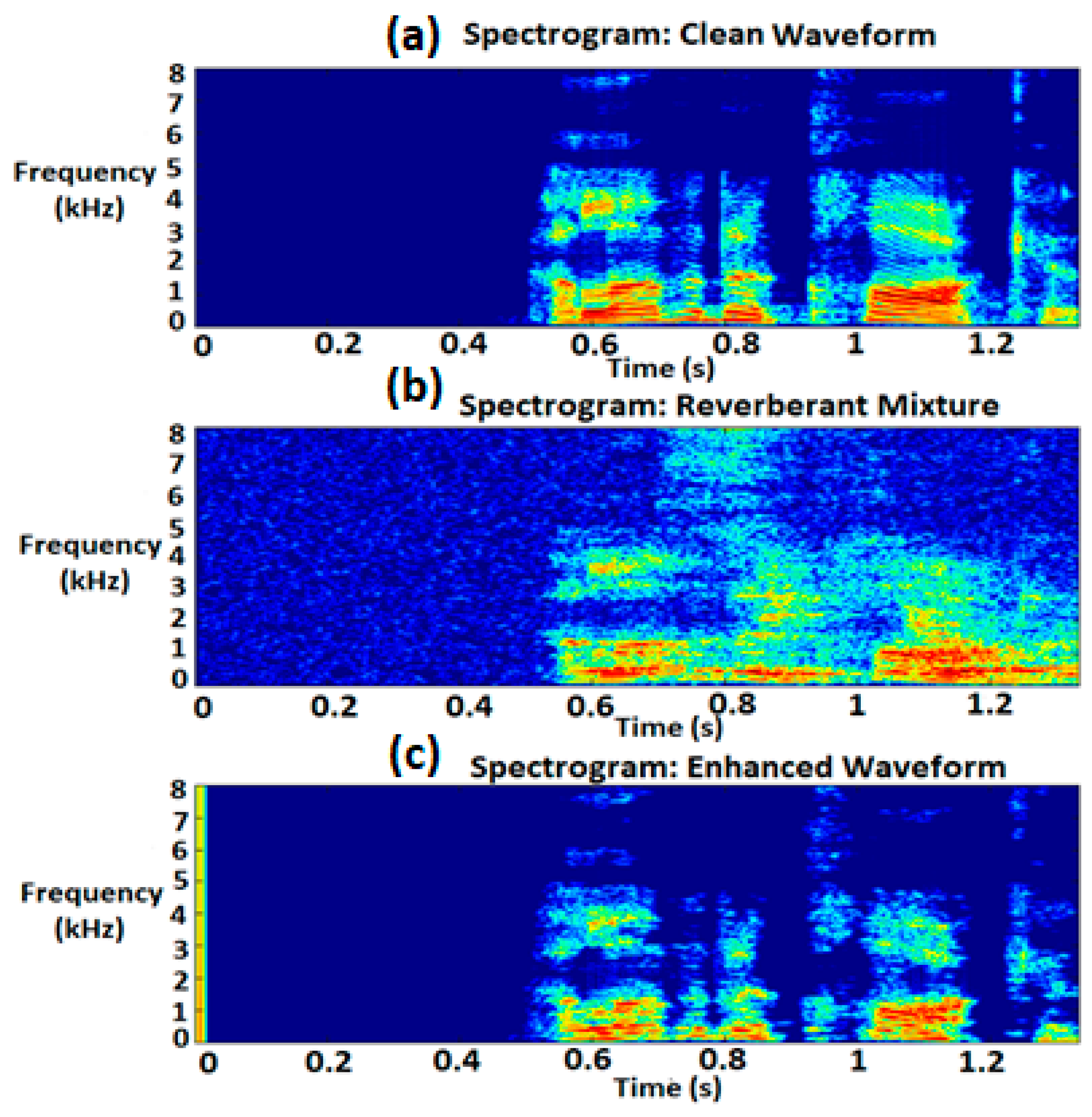
4.4.2. Performance Comparison of Proposed Approach on Simulated and Recorded RIRs

From Table 7, it is evident that the proposed approach of the residual dense Graph-U-Net, assisted by MS-GLMB filtering, outperforms the other state-of-the-art approaches of target speech enhancement under reverberant conditions, when the sources are in motion with intermittent speech activity. This is because the spectro-spatial features extracted by the MS-GLMB filtering framework provides training data for the proposed neural architecture by incorporating the effects of reverberation and motion of the sources, which helps the proposed neural architecture to learn the mapping from input spectro-spatial features to the target source-specific mask better than other approaches where a motion model of the speech sources is not considered.

In Table 8, ESTOI, PESQ, SI-SNR and SDR are used as the evaluation metrics of choice. Compared with STOI, ESTOI provides a more comprehensive assessment of the intelligibility of enhanced speech by considering additional factors such as additive and convolutional distortions that are commonly encountered in real-world scenarios.

As observed from Table 8, the TI_MVDR cannot handle the moving sources well because the estimated SCMs by TI_MVDR are time-invariant in nature, which causes the beamforming filter coefficients to also be time invariant. The online_MVDR method does appear to track moving sources but, in this approach, the tracking seems to depend on the forgetting factor that is responsible for providing exponentially less weight to the older ISCMs. Therefore, it is cumbersome to tune this parameter in order to offer optimal performance for various acoustic conditions that may arise during movements of the speech sources. The BLK_MVDR approach also suffers from sub-optimal performance due to the challenge involved in tuning the block sizes during online SCM computation. Because, during online operation, the objective is to perform beamforming based on an adequate number of signal samples received within a short time interval, it is challenging to tune the block size of received signals so as to provide optimal performance with this approach. The DOA_MVDR baseline approach serves as a benchmark for evaluating the performance of other beamforming approaches whereby an ‘oracle’ approach is designed with a priori knowledge of the DOAs. While it helps in performance evaluation, in practical scenarios, perfect knowledge of the DOAs cannot be obtained a priori because the estimated DOA information will be contaminated by noise imperfections. Finally, the mask-based MVDR beamformer approach with self-attention neural architecture seems to provide good performance under source movements due to the capability of the self-attention-based neural architecture to focus on a particular DOA direction. However, all of these beamforming approaches suffer from the assumption of a fixed cardinality of the sources, whereas the cardinality of the speech sources may vary due to the appearance and disappearances of the sources at different time frames within the acoustic environment. Due to the random nature of the cardinality, the MVDR beamformer needs to be dynamic in nature in order to be able to accurately steer the beam towards the target source while directing nulls towards the interfering sources at different time frames. In this regard, the proposed approach seems to outperform other state-of-the-art approaches of speech enhancement using DL techniques under reverberant conditions when all the sources are in motion. While the MS-GLMB-assisted source tracking helps in target source tracking across the time frames, the presence of dense convolutions with residual blocks in the neural architecture helps to cancel the noise better than conventional convolutional modules in the U-Net architecture. Moreover, the presence of GCRNN in the bottleneck of the overall U-Net helps to exploit the implicit information, such as spatial and temporal-spectral information, in a more flexible manner as compared with conventional methodologies. Speech enhancement methods based on conventional beamforming are sensitive to the motion of acoustic sources, which explains why the performance of the conventional GSC-based beamformer degrades in dynamic conditions. Estimation of the time-varying statistics, using labelled RFS-based algorithms and DL architectures, within the conventional beamforming pipeline (such as GSC-MVDR) lead to improved speech intelligibility and speech quality than the approaches without labelled RFS and DL methodology. This can be attributed to the fact that the labelled RFS-based algorithms provide a powerful framework to model the motion of the sources, which in turn leads to better construction of the dataset by considering the effects of time-varying interference and multipath impairments such as reverberation with higher accuracy. From Table 7 and Table 8, it is evident that the performance of the integrated MS-GLMB filtering-assisted neural beamforming is superior to other neural speech enhancement methods under reverberant conditions when the sources are in motion.

Unlike the results in Table 7 and Table 8, which were based on simulated RIRs, in this sub-section, we outline the results of the application of the proposed approach to recorded RIRs. The Aachen impulse response (AIR) [57] database is used for selecting the recorded RIRs, in this case two RIRs, recorded from office and corridor environments and with RT60 = 0.52 s and 1.25 s respectively. Moreover, noise samples from the DEMAND database were added to these RIRs to create a noisy, reverberant dataset at a low acoustic SNR of 0 dB.

As observed from Table 9, the proposed neural approach also outperforms other methods of speech enhancement in terms of objective quality metrics under recorded RIRs. This indicates that the proposed method is also able to generalize well to recorded RIRs, under noisy conditions.

4.4.3. ANOVA Analysis

In this sub-section, we confirm the significance of the results achieved using the proposed speech enhancement approach over other methods using the analysis-of-variance (ANOVA) approach. The statistical tests were conducted at a 95% confidence interval. The differences between achieved ESTOI and PESQ using the proposed method and other approaches are considered to be significant if the probability value denoted by the p-value is less than 0.05 and if the F-value of the Fisher–Snedecor distribution (also referred to as the F-distribution) is higher than its critical value (F-critical).

Table 10. ANOVA analysis of speech enhancement methods at 95% confidence interval.

Speech Enhancement Approach	PESQ		ESTOI
	p-Value	F-Value	p-Value	F-Value
Proposed approach -> noisy speech	0.001	50.25	0.001	54.24
Proposed approach -> MS-GLMB filtering-assisted MVDR beamformer	0.023	12.17	0.042	09.45
Proposed approach -> mask MVDR with self-attention	0.021	20.07	0.031	15.15
Proposed approach -> U-Net with embedded GCN	0.012	14.76	0.039	12.15

presents the results of the statistical test at a 95% confidence interval with the value of F-critical at 4.10.

From the results presented in Table 10, it is clear that the results are statistically significant, and that the proposed approach consistently outperforms prior state-of-the-art approaches in terms of speech intelligibility and quality (represented by ESTOI and PESQ metrics, respectively).

4.4.4. Ablation Study

In order to investigate the contribution of different components in the proposed neural speech enhancement architecture, in this sub-section we conduct an ablation study. In this study, we compare variants of the proposed speech enhancement approach whereby the results are presented in

Table 11. Results of ablation study.

Method	RT60 = 550 ms		RT60 = 250 ms		RT60 = 50 ms
	PESQ	ESTOI	PESQ	ESTOI	PESQ	ESTOI
Proposed approach	2.70	75.00%	2.88	79.60%	2.90	80.50%
w/o GCRNN block in skip connections	2.65	72.60%	2.84	76.70%	2.87	78.40%
w/o Residual block in encoder and decoder	2.57	69.50%	2.75	72.22%	2.78	76.32%
w/o Discriminator	2.67	74.43%	2.85	77.45%	2.89	79.20%

.

In Table 11, the PESQ and ESTOI values corresponding to variants of the proposed approach are listed, and these clearly demonstrate the superior performance achieved by the proposed approach. The entry ‘w/o GCRNN block in skip connections’ indicates that the GCRNN blocks were removed from the skip connections of the overall U-Net architecture, while including the GCRNN in the bottleneck layer of the U-Net. There is a decrease in PESQ value by 0.05 for the reverberation time RT60 of 550 ms after the removal of the GCRNN blocks from the skip connections, which is due to reduction in feature extraction capability of the neural architecture. As the GCRNN block in the bottleneck layer is still left unchanged, some degree of flexibility in the exploitation of spatiotemporal and spectral information is still maintained. There is also a slight reduction in ESTOI value due to removal of the GCRNN blocks from the skip connections, which indicates a slight reduction in speech intelligibility. The entry ‘w/o Residual block in Encoder and Decoder’ in Table 11 indicates the removal of residual blocks from the encoder and decoder pathways of the U-Net architecture while keeping other components intact. It is evident that the removal of residual blocks leads to loss of feature preservation in the overall neural architecture, which is why the PESQ and ESTOI values become diminished. The entry ‘w/o Discriminator’ refers to the case in which the discriminator of the GAN framework is removed. As expected, the PESQ and ESTOI values are reduced as compared with the original proposed approach, as the non-GAN neural framework is incapable of discriminating between the original desired signal and the noisy received signal at the input and is also prone to adversarial conditions.

5. Discussion

The MS-GLMB filtering can solve the space-time permutation problem. Hence, its application in the source tracking-assisted beamforming procedure is useful to generate the labels (i.e., identities) of the multiple sources, along with their location estimates, across all of the time frames, with high accuracy even under low SNR and high reverberation and while sources change their positions and speak intermittently. The estimated labels are instrumental in correctly discriminating between the target speech source and interferers, which facilitate the construction of time-varying MVDR beamformers and subsequent T-F mask corresponding to the target source. This in turn can enhance the target speech in a dynamic manner within each time frame, even under the combined effect of imperfections caused by the sources’ motion, reverberation and background noise. The T-F masks thus generated form an effective target label set for the proposed neural architecture, which is robust to imperfections caused by background noise, reverberation and motion of the sources. As an appropriate motion model such as the Langevin model is considered in modelling the motion of the sources while implementing the MS-GLMB filter, the dynamic changes in positions of the mobile sources are accounted for, which is reflected in the training procedure of the proposed residual dense Graph-U-Net-based neural speech enhancement model. In prior works concerning speech enhancement using deep neural architectures [8,9,10,11,12,13,14,15,16,17,18,19,20,21,22,23,24,25,26,27,28,29,30], the dynamics of the sources in motion using appropriate motion models were not considered, which is why the state-of-the-art deep neural architectures employed in prior research works may not provide satisfactory performance under the combined effect of imperfections caused by reverberation, noise and interfering sources. As evident in this work, the label generation procedure for training the neural architecture considers the sources’ motion, whose trajectories possess different start and termination points as well as different velocities. Moreover, the circumvention of the space-time permutation problem by the MS-GLMB filtering leads to correct discrimination between the target source and the interfering sources across all of the time frames, which in turn assists the training label generation procedure to generate the T-F masks with high accuracy. The proposed neural framework effectively learns the mapping from the spectrograms corresponding to a received multichannel reverberant mixture of speech signals belonging to the multiple sources at different spatial positions to the T-F mask corresponding to the target source. Through this overall procedure, the knowledge about the sources’ spatial information, as well as the dynamic beamformer’s operation within each time frame, are implicitly included within the training procedure of the proposed neural framework, which enables the trained version to generalize to unseen conditions such as different RIRs, SNRs and variations in the sources’ motion. While the research work outlined in [18,19,20], relying on “complex spectral mapping,” as well as the research works in [14,15], aim to predict the target source-specific mask to enhance the target speech, as mentioned earlier they do not consider the motion of the sources, nor do they consider the random nature of the cardinality of the sources while training the respective neural architectures. Hence, compared with those approaches, the approach presented in this article performs better under dynamic conditions.

As pointed out in [19,25,42,43], the goal of dense connections is to maximize the information processing from all layers, whereas the inclusion of residual connections leads to an improved utilization of information as well as preservation of signal integrity. The combination of dense and residual connections leads to the formation of the residual dense block which improves the network efficiency. This in turn ensures an enhancement in the fusion of feature information. While similar approaches of target speech enhancement using GCN have been reported, this work embeds a GCRNN module in a residual dense convolutional U-Net framework, which is different from the neural architectures adopted in [27,28,29].

6. Application Scenarios of the Proposed Approach

In this sub-section, we outline a few applications for which the proposed speech enhancement approach can be leveraged.

6.1. Applications in Conferencing Scenarios

During video conferencing, the quality of speech can become severely degraded due to background noise, reverberation, the number of recording microphones, the geometry of the microphone array, the acoustic and circuit design of the microphone arrays, the interference due to speakers, etc. [58]. Therefore, speech enhancement is a critical component of the overall speech processing system and plays an important role in video conferencing applications. As compared with a microphone placed very close to a speaker, microphone arrays offer better speech intelligibility by offering significant directional gain as well as effective noise reduction, thereby leading to an improvement in overall audio experience for the participants in the conference. Due to the motion of the speakers, it is necessary to track them and switch the focus towards the desired speaker in a dynamic manner. For this reason, microphone array-based speech enhancement techniques which incorporate localization and tracking methods are ideal for ensuring clear and intelligible communication in conference rooms, rooms which involve participants changing their positions or intermittently speaking from different locations. The proposed approach in this paper involves multiple microphone arrays with an MS-GLMB filtering algorithm to track the speakers and deep neural architecture-based speech enhancement. Such an approach can be leveraged to dynamically enhance the targeted speech in a conference environment.

6.2. Applications in Assistive Listening Devices

The proposed approach can be leveraged to assistive listening devices such as hearing aids in order to improve the overall audio experience of the listener. Due to the distributed nature of the multi-microphone array configuration used in this work, it possesses the advantages of spatial diversity, enhanced noise reduction performance, and flexibility of placement. Spatial diversity indicates the placement of microphones at different positions which can enable the speech enhancement system to distinguish between the speech emanating from the target source and interfering signals and noise arriving from different directions. This can, in turn, help the system to isolate and enhance the desired speech signal while suppressing undesired components. The enhanced noise reduction performance can be attributed to beamforming, which helps to focus on a speech signal arriving from a specific direction while suppressing other directions. Finally, owing to its distributed nature, the microphone array elements can be flexibly placed across the user’s clothing, or they can be distributed across the indoor environment, so as to effectively capture the acoustic signals from different directions [59]. The proposed approach, if leveraged to a distributed microphone array-based hearing aid application, can localize the speech source-of-interest at each time frame and improve the intelligibility of speech by performing dynamic beamforming-based target speech enhancement.

6.3. Applications in Automatic Speech Recognition for Speakers in Motion

Automatic speech recognition is a crucial step in the overall speech processing pipeline, one which requires the application of appropriate speech enhancement technique to improve speech intelligibility. This is most critical in scenarios involving moving speakers who change their positions across different time frames while speaking intermittently. The movement of speakers introduces additional challenges, such as changing acoustics, noise, as well as motion-induced acoustic impairments which hamper accurate recognition of the received speech signal. Automatic speech recognition is an important procedure in speech transcription systems [60]. The proposed technique can be leveraged to such scenarios where the source tracking assisted neural beamformer can effectively isolate the desired speech component from the interference signals, thereby leading to better recognition of the target speech as well as better transcription.

7. Conclusions

In this research work, a deep neural architecture for enhancing the target speech under reverberant conditions is proposed, whereby the training labels are created by exploiting the spatial information of the sources across all of the time frames using MS-GLMB filtering. Such an approach helps to correctly discriminate between the target source and interfering sources and the overall methodology demonstrates better performance in scenarios in which the sources are in motion than state-of-the-art neural speech enhancement methods which do not employ MS-GLMB filtering. The positive outcome of the proposed methodology lies in the incorporation of the spectro-spatial information within the training procedure of the neural architecture, which enables the trained neural architecture to directly predict the desired T-F masks from the input magnitude spectrograms even under “un-seen” acoustic conditions, such as different RIRs, SNRs and sources’ motion, which were not included in the training phase.

8. Future Work

As mentioned in the article, the methodology exploits the SRP-PHAT-based acoustic measurements for constructing the measurement set for the MS-GLMB filter. While the tracking performance is generally good in the presence of noise and reverberation, it can be further improved by modeling the SRP-PHAT computation by a suitable deep neural architecture. Such a neural SRP approach can provide increased noise immunity to the localization and tracking procedure, which can lead to improved reliability under sources’ motions as well as background noise and reverberation. This in turn can lead to better target source separation by the MVDR beamformer module.

The proposed neural architecture can be leveraged in audio-visual information-guided target speech enhancement, where the visual tracking of the target speech source can be assisted by a neural acoustic localization. Such a neural localization framework can benefit from the residual dense convolutional Graph-U-Net applied in this work. Moreover, the proposed neural framework can also be incorporated within the audio-visual speech enhancement module.

References

1. Brendel, A.; Haubner, T.; Kellermann, W. A Unifying View on Blind Source Separation of Convolutive Mixtures Based on Independent Component Analysis. IEEE Trans. Sig. Proc. 2023, 71, 816–830. [Google Scholar] [CrossRef]
2. Wang, T.; Yang, F.; Yang, J. Convolutive Transfer Function-Based Multichannel Nonnegative Matrix Factorization for Overdetermined Blind Source Separation. IEEE/ACM Trans. Audio Speech Lang. Proc. 2022, 30, 802–815. [Google Scholar] [CrossRef]
3. Nionm, D.; Mokios, K.N.; Sidiropoulos, N.D.; Potamianos, A. Batch and Adaptive PARAFAC-based Blind Separation of Convolutive Speech Mixtures. IEEE Trans. Audio Speech Lang. Proc. 2010, 18, 1193–1207. [Google Scholar] [CrossRef]
4. Gannot, S.; Vincent, E.; Markovich-Golan, S.; Ozerov, A. A consolidated perspective on multimicrophone speech enhancement and source separation. IEEE/ACM Trans. Audio Speech Lang. Proc. 2017, 25, 692–730. [Google Scholar] [CrossRef]
5. Markovich-Golan, S.; Gannot, S.; Kellermann, W. Combined LCMV-TRINICON Beamforming for Separating Multiple Speech Sources in Noisy and Reverberant Environments. IEEE/ACM Trans. Audio Speech Lang. Proc. 2016, 25, 320–332. [Google Scholar] [CrossRef]
6. Ong, J.; Vo, B.T.; Nordholm, S. Blind Separation for Multiple Moving Sources with Labeled Random Finite Sets. IEEE/ACM Trans. Audio Speech Lang. Proc. 2021, 29, 2137–2151. [Google Scholar] [CrossRef]
7. Morgan, J.P. Time-Frequency Masking Performance for Improved Intelligibility with Microphone Arrays. Master’s Thesis, University of Kentucky, Lexington, KY, USA, 2017. [Google Scholar]
8. Ochiai, T.; Delcroix, M.; Nakatani, T.; Araki, S. Mask-Based Neural Beamforming for Moving Speakers with Self-Attention-Based Tracking. IEEE/ACM Trans. Audio Speech Lang. Proc. 2023, 31, 835–848. [Google Scholar] [CrossRef]
9. Tammen, M.; Ochiai, T.; Delcroix, M.; Nakatani, T.; Araki, S.; Doclo, S. Array Geometry-Robust Attention-Based Neural Beamformer for Moving Speakers. arXiv 2024, arXiv:2402.03058. [Google Scholar]
10. Wang, Y.; Politis, A.; Virtanen, T. Attention-Driven Multichannel Speech Enhancement in Moving Sound Source Scenarios. In Proceedings of the 2024 IEEE International Conference on Acoustics, Speech and Signal Processing (ICASSP), Seoul, Republic of Korea, 14–19 April 2024. [Google Scholar]
11. Xu, Y.; Yu, M.; Zhang, S.; Chen, L.; Weng, C.; Liu, J.; Yu, D. Neural Spatio-Temporal Beamformer for Target Speech Separation. In Proceedings of the INTERSPEECH 2020, Shanghai, China, 25–29 October 2020. [Google Scholar]
12. Xu, Y.; Zhang, Z.; Yu, M.; Zhang, S.-X.; Yu, D. Generalized Spatio-Temporal RNN Beamformer for Target Speech Separation. In Proceedings of the INTERSPEECH 2021, Brno, Czech Republic, 30 August–3 September 2021. [Google Scholar]
13. Guo, A.; Wu, J.; Gao, P.; Zhu, W.; Guo, Q.; Gao, D.; Wang, Y. Enhanced Neural Beamformer with Spatial Information for Target Speech Extraction. In Proceedings of the 2023 Asia Pacific Signal and Information Processing Association Annual Summit and Conference (APSIPA ASC) 2023, Taipei, Taiwan, 31 October–3 November 2023. [Google Scholar]
14. Tan, K.; Wang, Z.-Q.; Wang, D. Neural spectrospatial filtering. IEEE/ACM Trans. Audio Speech Lang. Proc. 2022, 30, 605–621. [Google Scholar] [CrossRef]
15. Wang, Z.-Q.; Wang, D. Combining spectral and spatial features for deep learning based blind speaker separation. IEEE/ACM Trans. Audio Speech Lang. Proc. 2019, 27, 457–468. [Google Scholar] [CrossRef]
16. Zhang, Z.; Xu, Y.; Yu, M.; Zhang, S.-X.; Chen, L.; Yu, D. ADLMVDR: All deep learning MVDR beamformer for target speech separation. In Proceedings of the 2021 IEEE International Conference on Acoustics, Speech and Signal Processing (ICASSP), Toronto, ON, Canada, 6–11 June 2021. [Google Scholar]
17. Gu, R.; Chen, L.; Zhang, S.-X.; Zheng, J.; Xu, Y.; Yu, M.; Su, D.; Zou, Y.; Yu, D. Neural spatial filter: Target speaker speech separation assisted with directional information. In Proceedings of the INTERSPEECH 2019, Graz, Austria, 15–19 September 2019. [Google Scholar]
18. Luo, Y.; Mesgarani, N. Conv-TasNet: Surpassing ideal time-frequency magnitude masking for speech separation. IEEE/ACM Trans. Audio Lang. Proc. 2019, 27, 1256–1266. [Google Scholar] [CrossRef]
19. Tolooshams, B.; Giri, R.; Song, A.H.; Isik, U.; Krishnaswamy, A. Channel-Attention Dense U-Net for Multichannel Speech Enhancement. In Proceedings of the 2020 IEEE International Conference on Acoustics, Speech and Signal Processing (ICASSP), Barcelona, Spain, 4–8 May 2020. [Google Scholar]
20. Nair, A.A.; Reiter, A.; Zheng, C.; Nayar, S. Audiovisual Zooming: What You See Is What You Hear. In Proceedings of the 27th ACM International Conference on Multimedia, Nice, France, 21–25 October 2019. [Google Scholar]
21. Soni, M.H.; Shah, N.; Patil, H.A. Time-Frequency Masking-Based Speech Enhancement Using Generative Adversarial Network. In Proceedings of the 2018 IEEE International Conference on Acoustics, Speech and Signal Processing (ICASSP), Calgary, AB, Canada, 15–20 April 2018. [Google Scholar]
22. Baby, D. iSEGAN: Improved Speech Enhancement Generative Adversarial Networks. arXiv 2020, arXiv:2002.08796v1. [Google Scholar] [CrossRef]
23. Michelsanti, D.; Tan, Z.-H. Conditional Generative Adversarial Networks for Speech Enhancement and Noise-Robust Speaker Verification. In Proceedings of the INTERSPEECH 2017, Stockholm, Sweden, 20–24 August 2017. [Google Scholar]
24. Pascual, S.; Bonafonte, A.; Serrà, J. SEGAN: Speech Enhancement Generative Adversarial Network. arXiv 2017, arXiv:1703.09452v3. [Google Scholar] [CrossRef]
25. Zhou, L.; Zhong, Q.; Wang, T.; Lu, S.; Hu, H. Speech Enhancement via Residual Dense Generative Adversarial Network. Comp. Sys. Sci. Eng. 2021, 38, 279–289. [Google Scholar] [CrossRef]
26. Datta, J.; Firoozabadi, A.D.; Zabala-Blanco, D.; Soria, F.R.C.; Adams, M.; Perez, C. Multi-channel Target Speech Enhancement using Labeled Random Finite Sets and Deep Learning under Reverberant Environments. In Proceedings of the 2023 IEEE 5th Eurasia Conference on IOT, Communication and Engineering (ECICE), Yunlin, Taiwan, 27–29 October 2023. [Google Scholar]
27. Binh, N.H.; Hai, D.V.; Dat, B.T.; Chau, H.N.; Cuong, N.Q. Multi-channel speech enhancement using a minimum variance distortionless response beamformer based on graph convolutional network. Int. J. Adv. Comput. Sci. Appl. 2022, 13, 739–747. [Google Scholar] [CrossRef]
28. Chau, H.N.; Bui, T.D.; Nguyen, H.B.; Duong, T.T.H.; Nguyen, Q.C. A Novel Approach to Multi-Channel Speech Enhancement Based on Graph Neural Networks. IEEE/ACM Trans. Audio Speech Lang. Proc. 2024, 32, 1133–1144. [Google Scholar] [CrossRef]
29. Tzirakis, P.; Kumar, A.; Donley, J. Multi-channel speech enhancement using graph neural networks. Proceedings of 2021 the IEEE International Conference on Acoustics, Speech and Signal Processing (ICASSP), Toronto, ON, Canada, 6–11 June 2021. [Google Scholar]
30. Zhang, C.; Xiang, P. Single-channel speech enhancement using Graph Fourier Transform. In Proceedings of the INTERSPEECH 2022, Incheon, Republic of Korea, 18–22 September 2022. [Google Scholar]
31. Ong, J.; Vo, B.T.; Nordholm, S.; Vo, B.-N.; Moratuwage, D.; Shim, C. Audio-Visual Based Online Multi-Source Separation. IEEE/ACM Trans. Audio. Speech. Lang. Proc. 2022, 30, 1219–1234. [Google Scholar] [CrossRef]
32. Vo, B.-N.; Vo, B.-T.; Beard, M. Multi-sensor multi-object tracking with the generalized labeled multi-bernoulli filter. IEEE Trans. Signal Process. 2019, 67, 5952–5967. [Google Scholar] [CrossRef]
33. Thomas, R.W.; Larson, J.D. Inverse Reinforcement Learning for Generalized Labeled Multi-Bernoulli Multi-Target Tracking. In Proceedings of the 2021 IEEE Aerospace Conference (50100), Big Sky, MT, USA, 6–13 March 2021. [Google Scholar]
34. Jiang, D.; Qu, H.; Zhao, J. Multi-level graph convolutional recurrent neural network for semantic image segmentation. Telecom. Sys. 2021, 77, 563–576. [Google Scholar] [CrossRef]
35. Goodfellow, I.J.; Abadie, J.P.; Mirza, M.; Xu, B.; Farley, D.W.; Ozair, S.; Courville, A.; Bengio, Y. Generative Adversarial Networks. arXiv 2014, arXiv:1406.2661v1. [Google Scholar] [CrossRef]
36. Pan, Z.; Yu, W.; Yi, X.; Khan, A.; Yuan, F.; Zheng, Y. Recent Progress on Generative Adversarial Networks (GANs): A Survey. IEEE Access. 2019, 7, 36322–36333. [Google Scholar] [CrossRef]
37. Marques, A.G.; Kiyavash, N.; Moura, J.M.F.; Van De Ville, D.; Willett, R. Graph Signal Processing: Foundations and Emerging Directions [From the Guest Editors]. IEEE Sig. Proc. Mag. 2020, 37, 11–13. [Google Scholar] [CrossRef]
38. Li, G.; Muller, M.; Thabet, A.; Ghanem, B. DeepGCNs: Can GCNs go as deep as CNNs? In Proceedings of IEEE/CVF International Conference on Computer Vision, Seoul, Republic of Korea, 27 October–2 November 2019.
39. Seo, Y.; Defferrard, M.; Vandergheynst, P.; Bresson, X. Structured Sequence Modeling with Graph Convolutional Recurrent Networks. arXiv 2016, arXiv:1612.07659. [Google Scholar] [CrossRef]
40. Ronneberger, O.; Fischer, P.; Brox, T. U-Net: Convolutional Networks for Biomedical Image Segmentation. In Medical Image Computing and Computer-Assisted Intervention–MICCAI 2015, Proceedings of the MICCAI 2015, Munich, Germany, 5–9 October 2014; Navab, N., Hornegger, J., Wells, W., Frangi, A., Eds.; Lecture Notes in Computer Science 9351; Springer: Cham, Switzerland, 2014. [Google Scholar] [CrossRef]
41. He, K.; Zhang, X.; Ren, S.; Sun, J. Deep Residual Learning for Image Recognition. arXiv 2015, arXiv:1512.03385v1. [Google Scholar] [CrossRef]
42. Zhang, Z.; Liu, Q.; Wang, Y. Road Extraction by Deep Residual U-Net. IEEE Geosci. Remote Sens. Lett. 2018, 15, 749–753. [Google Scholar] [CrossRef]
43. Yang, X.; Li, X.; Ye, Y.; Zhang, X.; Zhang, H.; Huang, X. Road Detection via Deep Residual Dense U-Net. In Proceedings of the 2019 International Joint Conference on Neural Networks (IJCNN), Budapest, Hungary, 14–19 July 2019. [Google Scholar]
44. Huang, G.; Liu, Z.; van der Laurens, M.; Weinberger, K.Q. Densely connected convolutional networks. In Proceedings of the 2017 IEEE Conference on Computer Vision and Pattern Recognition, Piscataway, NJ, USA, 21–26 July 2017. [Google Scholar]
45. Datta, J.; Adams, M.; Perez, C. Dense-U-Net assisted Localization of Speech Sources in Motion under Reverberant conditions. In Proceedings of the 2023 12th International Conference on Control, Automation and Information Sciences (ICCAIS), Hanoi, Vietnam, 27–29 November 2023. [Google Scholar] [CrossRef]
46. Do, H.; Silverman, H.F.; Yu, Y. A real-time SRP-PHAT source location implementation using stochastic region contraction (SRC) on a large-aperture microphone array. In Proceedings of the 2007 IEEE International Conference on Acoustics, Speech, and Signal Processing (ICASSP), Honolulu, HI, USA, 16–20 April 2007. [Google Scholar]
47. Paul, D.B.; Baker, J. The design for the wall street journal-based CSR corpus. In Proceedings of the 1992 Workshop on Speech and Natural Language, Harriman, NY, USA, 23–26 February 1992. [Google Scholar]
48. Panayotov, V.; Chen, G.; Povey, D.; Khudanpur, S. Librispeech: An ASR corpus based on public domain audio books. In Proceedings of the 2015 IEEE International Conference on Acoustics, Speech and Signal Processing (ICASSP), South Brisbance, QLD, Australia, 19–24 April 2015. [Google Scholar]
49. Barker, J.; Marxer, R.; Vincent, E.; Watanabe, S. The third ‘CHiME’ speech separation and recognition challenge: Dataset, task and baselines. In Proceedings of the 2015 IEEE Workshop on Automatic Speech Recognition and Understanding (ASRU), Scottsdale, AZ, USA, 13–17 December 2015. [Google Scholar]
50. Thiemann, J.; Ito, N.; Vincent, E. The diverse environments multichannel acoustic noise database: A database of multichannel environmental noise recordings. J. Acoust. Soc. Am. 2013, 133, 3591. [Google Scholar] [CrossRef]
51. Piczak, K.J. ESC: Dataset for Environmental Sound Classification. In Proceedings of the 23rd Annual ACM Conference on Multimedia, Brisbane, Australia, 26–30 October 2015. [Google Scholar]
52. Jensen, J.; Taal, C.H. An algorithm for predicting the intelligibility of speech masked by modulated noise maskers. IEEE/ACM Trans. Audio Speech Lang. Proc. 2016, 24, 2009–2022. [Google Scholar] [CrossRef]
53. Rix, A.W.; Beerends, J.G.; Hollier, M.P.; Hekstra, A.P. Perceptual evaluation of speech quality (PESQ)-a new method for speech quality assessment of telephone networks and codecs. In Proceedings of the 2001 IEEE International Conference on Acoustics, Speech, Signal Processing, Salt Lake City, UT, USA, 7–11 May 2001. [Google Scholar]
54. Le Roux, J.; Wisdom, S.; Erdogan, H.; Hershey, J.R. SDR–half-baked or well done? In Proceedings of 2019 IEEE International Conference on Acoustics, Speech, Signal Processing (ICASSP), Brighton, UK, 12–17 May 2019.
55. Lehmann, E.A.; Johansson, A.M.; Nordholm, S. Reverberation-time prediction method for room impulse responses simulated with the image source model. In Proceedings of the 2007 IEEE Workshop on Applications of Signal Processing to Audio and Acoustics, New Paltz, NY, USA, 21–24 October 2007. [Google Scholar]
56. Kingma, D.P.; Ba, J. Adam: A method for stochastic optimization. arXiv 2014, arXiv:1412.6980. [Google Scholar]
57. Jeub, M.; Sch¨afer, M.; Kr¨uger, H.; Nelke, C.; Beaugeant, C.; Vary, P. Do we need dereverberation for hand-held telephony? In Proceedings of 2010 International Congress on Acoustics (ICA), Sydney, Australia, 23–27 August 2010.
58. Rao, W.; Fu, Y.; Hu, Y.; Xu, X.; Jv, Y.; Han, J.; Jiang, Z.; Xie, L.; Wang, Y.; Watanabe, S.; et al. Conferencingspeech Challenge: Towards Far-Field Multi-Channel Speech Enhancement for Video Conferencing. In Proceedings of the 2021 IEEE Automatic Speech Recognition and Understanding Workshop (ASRU), Cartagena, Colombia, 13–17 December 2021; IEEE: Piscataway, NJ, USA, 2021; pp. 679–686. [Google Scholar] [CrossRef]
59. Pasha, S.; Lundgren, J.; Ritz, C.; Zou, Y. Distributed Microphone Arrays, Emerging Speech and Audio Signal Processing Platforms: A Review. Adv. Sci. Technol. Eng. Syst. J. 2020, 5, 331–343. [Google Scholar] [CrossRef]
60. Audhkhasi, K.; Georgiou, P.G.; Narayanan, S.S. Analyzing quality of crowd-sourced speech transcriptions of noisy audio for acoustic model adaptation. In Proceedings of the 2012 IEEE International Conference on Acoustics, Speech and Signal Processing (ICASSP), Kyoto, Japan, 25–30 March 2012; IEEE: Piscataway, NJ, USA, 2012; pp. 4137–4140. [Google Scholar] [CrossRef]
Figure 1. Target speech enhancement with MS-GLMB filtering-assisted covariance mask prediction and GSC-based D-S beamformer [26].
Applsci 15 02944 g001
Figure 2. T-F mask prediction using a spectro-spatial feature set (constructed from input multichannel spectrogram and location information obtained by MS-GLMB filtering) and proposed residual dense convolutional graph-U-Net framework (training phase).
Applsci 15 02944 g002
Figure 3. T-F mask by the proposed residual dense convolutional graph-U-Net framework (testing phase).
Applsci 15 02944 g003
Figure 4. Architecture of the RDB utilized within each layer of encoder and decoder of the residual dense Graph-U-Net (The different colors denote the dense interconnections between convolutional layers within the dth residual block).
Applsci 15 02944 g004
Figure 5. Prediction of T-F mask using the residual dense convolution-based Graph-U-Net framework for speech enhancement.
Applsci 15 02944 g005
Figure 6. Plot of estimated (x-, y-) coordinates by MS-GLMB filter across all time frames at reverberation time RT60 = 550 ms and acoustic SNR = 35 dB. The colored tracks in the form of straight lines indicate the original i.e., ground truth trajectories corresponding to 3 speech sources, whereas the colored tracks with dots indicate estimates of the source trajectories obtained by the MS-GLMB filter.
Applsci 15 02944 g006
Figure 7. (a) Spectrogram of the clean speech signal belonging to the target source, (b) spectrogram of the reverberant mixture of speech signals corresponding to 3 sources, (c) spectrogram of the enhanced speech signal corresponding to target source. The colored portion of the spectrograms between 0.5 s and 1.3 s denote the presence of speech (All speech signals belong to LibriSpeech dataset).
Applsci 15 02944 g007
Figure 8. (a) Spectrogram of the clean speech signal belonging to the target source, (b) spectrogram of the reverberant mixture of speech signals corresponding to 3 sources, (c) spectrogram of enhanced speech signal corresponding to the target source. The colored portion of the spectrograms between 0.5 s and 1.3 s denote the presence of speech (All speech signals belong to WS2J0 dataset).
Applsci 15 02944 g008