Abstract
Modern imaging systems produce a great volume of image data. In many practical situations, it is necessary to compress them for faster transferring or more efficient storage. Then, a compression has to be applied. If images are noisy, lossless compression is almost useless, and lossy compression is characterized by a specific noise filtering effect that depends on the image, noise, and coder properties. Here, we considered a modern HEIF coder applied to grayscale (component) images of different complexity corrupted by additive white Gaussian noise. It has recently been shown that an optimal operation point (OOP) might exist in this case. Note that the OOP is a value of quality factor where the compressed image quality (according to a used quality metric) is the closest to the corresponding noise-free image. The lossy compression of noisy images leads to both noise reduction and distortions introduced into the information component, thus, a compromise should be found between the compressed image quality and compression ratio attained. The OOP is one possible compromise, if it exists, for a given noisy image. However, it has also recently been demonstrated that the compressed image quality can be significantly improved if post-filtering is applied under the condition that the quality factor is slightly larger than the one corresponding to the OOP. Therefore, we considered the efficiency of post-filtering where a block-matching 3-dimensional (BM3D) filter was applied. It was shown that the positive effect of such post-filtering could reach a few dB in terms of the PSNR and PSNR-HVS-M metrics. The largest benefits took place for simple structure images and a high intensity of noise. It was also demonstrated that the filter parameters have to be adapted to the properties of residual noise that become more non-Gaussian if the compression ratio increases. Practical recommendations on the use of compression parameters and post-filtering are given.
1. Introduction and Related Work
An obvious tendency in modern computer vision (CV), remote sensing (RS), and medical diagnostics (MD) is the increased number of acquired images and their size [1,2,3,4]. For some applications, the acquired images should be processed and passed to potential customers or decision undertaking systems quite quickly. For other practical situations, the acquired data have to be effectively saved for their future use such as in medical and multitemporal imaging [3,5]. In these cases, efficient compression may be needed [5,6,7].
Existing compression techniques can be divided into two large groups: lossless [6] and lossy [7]. Both are widely used depending on the application, priority of requirements, and imposed restrictions. Lossless compression methods introduce no distortions into compressed images (data) but the produced compression ratio (CR) is usually not large (especially for images contaminated by noise) and cannot be varied (for given data, it can only be slightly improved by using a more efficient coder). If the attained CR is not appropriate, one has to apply a lossy compression technique [7,8,9]. The advantages of the compression techniques in this group consist of a considerably larger attained CR and a possibility of its variation, however, this is at the expense of distortions being introduced. A typical situation is that a larger produced CR leads to larger distortions that can become inappropriate or even annoying [1,8]. Then, one has to provide a reasonable trade-off between the attained CR and quality of the lossy compressed images, which happens in optical RS [9] and medical [10] imaging. This takes place in SSIM-based optimization [11], approaches to compression based on the just noticeable difference (JND) [12], and a better portable graphics (BPG) coder [13]. Note that such a trade-off should often be provided quickly and with the appropriate accuracy [13,14].
A positive feature in this sense is that the dependences of a metric characterizing lossy compressed image quality (e.g., mean square error (MSE) and CR) on a parameter that controls compression (PCC), such as the quality factor (QF) for compression techniques JPEG and HEIF [15], are usually monotonous (e.g., the MSE increases if the QF decreases for the mentioned coders). This allows for a potential reaching of the desired metric value with better or worse accuracy depending on the coder used, PCC employed, the metric exploited in image quality characterization, the procedure used for PCC variation, etc. [16]. In some practical situations, it is possible to ensure the high accuracy of providing a desired metric value if the PCC values are not discrete [16], but at the expense of several iterations when multiple compressions/decompressions of a considered image are needed. In other situations, the provided accuracy is lower (but can still be appropriate) with less computational expenses [15,17]. One reason can be the discrete nature of PCC [17]; another reason could be the residual errors of a two-stage procedure [13,15] or metric value prediction [12]. It is worth noting here that distortions can be characterized by conventional metrics such as the MSE or peak signal-to-noise ratio (PSNR), visual quality metrics (e.g., SSIM [11]), and their visibility threshold (see the just noticeable distortion (JND) concept in [12]). It is also possible to characterize introduced distortions by their impact on the classification or recognition of compressed images [11,18].
The described dependences and properties take place in lossy image compression if an image subject to compression is noise-free or, at the very least, the noise can hardly be noticed. However, for many classes of images, this assumption is not valid, for example, synthetic aperture radar (SAR) images that are always noisy due to speckle [19]. Conventional color images acquired in bad conditions can also be noisy [20]. A certain percentage of noisy (junk) component images are always present in hyperspectral [21] images. Noise also takes place in medical, night light, astronomic, and other images [22,23]. Some drones use cheap and low quality digital cameras, and as a result, the acquired images can also be noisy [24].
If a noisy image is subject to lossy compression, specific effects, discovered for SAR [25,26] and other images [27,28] about three decades ago, take place. The specific effect of noise reduction due to lossy compression was shown for both JPEG and wavelet-based techniques in [29,30] and [27,28], respectively. The concept of an optimal operation point (OOP) that can be observed was introduced in [28]. The OOP is the value of a used PCC when a minimal “distance” between the compressed and noise-free images is observed according to a considered quality metric. First, a possible OOP existence was demonstrated for conventional metrics such as PSNR; later, the possibility of OOP occurrence was shown [31] for many visual quality metrics including PSNR-HVS-M [32] and MS-SSIM [33]. For most metrics, the OOP relates to the global maximum, but there are a few metrics (MSE, MDSI [34]) for which the OOP corresponds to the global minimum.
As above-mentioned, the initial results concerning the OOP were obtained for JPEG and wavelet-based coders including JPEG2000 [35]. In state-of-the-art papers [36,37], a possible OOP existence was shown for coders based on discrete cosine transform (DCT) including a better portable graphics (BPG) coder [38,39]. Finally, the existence of an OOP has recently been demonstrated [17] for coders such as HEIF and AVIF [40], which are part of the video coder HEVC. In other words, it is possible to state that the existence of an OOP for some practical situations is typical for the lossy compression of noisy images including not only the case of pure additive noise, but also the case of signal-dependent noise [41]. Note that for many coders and noise types, fully automatic procedures for OOP determination have been proposed [37,41] based on the assumption that the noise type and characteristics are either known in advance or can be quite accurately estimated by the corresponding blind techniques for signal-dependent [42,43] and pure additive [44] noise types.
The OOP is not only a theoretical phenomenon, but also has considerable practical importance. An attractive advantage of the OOP is that, if an OOP exists for a given noisy image and a used coder, there is a certain sense of the image compressing in the OOP or its close neighborhood. Then, the benefit is twofold: good quality of the compressed image is provided, and the produced CR is quite large [17,36]. Meanwhile, two questions arise. First, there are images, coders, and noise intensities for which the OOP is absent (e.g., complex structure images corrupted by not very intensive noise). Then, there is how to set the coder PCC for such images to provide reasonably high CR and compressed image quality. Second, although the filtering effect in the OOP can be quite large, denoising due to lossy compression is not perfect. A good filter is able to provide an output PSNR that is a few dB larger than the PSNR in the OOP.
Keeping this in mind, an approach presuming a more “careful” (compared with the OOP) lossy compression combined with post-filtering applied to a decompressed image could be useful. Such an approach, to the best of our knowledge, was first proposed for DCT-based coders in [45,46]. Recently, a similar approach was studied for the BPG coder, where the DCT-based post-filtering was first analyzed [47], followed by the consideration of more complex non-local post-processing [48]. The post-processing of decompressed images is widely known [49,50], but the main goal for the corresponding methods is usually deblocking. The novelty of the approach in [47,48] consists of the fact that post-filtering after decompression was applied to remove residual noise for noisy images compressed by a modern BPG coder. In particular, the following has been shown:
- (1)
- A positive effect of post-filtering can be provided for images of different complexity under the condition that the CR is smaller than the CR for the OOP (parameter Q, which serves as the PCC for the BPG coder, is smaller than QOOP);
- (2)
- The optimal parameters of the DCT-based filter [51] change depending on Q and QOOP and noise intensity; general dependences can be found in [47];
- (3)
- The same has been observed [48] for the BM3D filter [52], where this filter, in general, performs slightly better than the DCT-based filter [47];
- (4)
- It is possible to predict the post-filter performance [48] and set its parameters in a way close to optimal; if Q increases, CR increases, but the general efficiency of post-filtering applied to decompressed images decreases; in this sense, Q ≈ QOOP-4 can be recommended for practical use.
Note here that the BPG and HEIF encoders have recently been proposed and can both be part of HEVC [7,53]. Moreover, the characteristics of BPG and HEIF in the case of the lossy compression of noisy images are very similar [17]. Meanwhile, the ways to find the OOP for the BPG and HEIF coders are different [17]. One way to find the OOP for HEIF was proposed in [17]. However, an opportunity to apply post-filtering for noisy images compressed by HEIF, to the best of our knowledge, has not been investigated yet. This was the main goal of this paper, and it deals with the novelty of the obtained results.
As a starting point, we considered the case of single-channel images contaminated by additive white Gaussian noise (AWGN) with a zero mean for the following reasons. AWGN is a standard noise model used in image processing applications such as the blind estimation of noise variance [44], filtering [54,55], and lossy compression [36,37]. If the noise observed in the original image is signal-dependent, it is possible to convert it to additive by using a proper variance stabilizing transform (VST) [17,56]. If such a VST is applied, lossy compression is employed after direct VST; the corresponding inverse transform should be used after decompression. Furthermore, although many modern images are multichannel nowadays [41,57], we focused on single-channel image lossy compression for two reasons. First, component-wise compression is still an easy way for volume reduction. Second, such a preliminary analysis of component-wise compression will, hopefully, bring an understanding of what should be conducted for multichannel data [41,57].
Summarizing the aforesaid, the novelty of this paper consists of the following:
- (1)
- To the best of our knowledge, the procedure of the post-filtering of noisy images lossy compressed by HEIF has never been considered, and the post-filtering of noisy images compressed by HEIF has several peculiarities given in the next items;
- (2)
- The filter choice is based on the presented statistical analysis of residual noise and introduced distortions where, to the best of our knowledge, such analysis has never been carried out;
- (3)
- The recommendations on setting the QF for the proposed compression procedure were based on the analysis results presented in Section 4.1 and Section 4.2. These recommendations differ from the recommendations for the BPG coder since the HEIF and BPG coders are controlled by different parameters (QF and Q) with different properties (CR increases if the QF becomes smaller for HEIF, and if Q increases for BPG, the QF varies in the limits from 1 to 100 whilst Q varies from 1 to 51, and so on);
- (4)
- Although the general tendencies of setting the post-filter parameter β appeared similar for the BPG and HEIF coders (for the larger CR optimal, β should be smaller), the obtained dependencies differed from the dependencies of different metrics on Q and β for the BPG coder presented in our earlier paper [47,48].
The rest of this paper is structured as follows. The image/noise model and the fundamental rate/distortion dependencies are considered in Section 2. A brief analysis of residual noise and distortions after the lossy compression of noisy images by HEIF are given in Section 3. The performance of post-filtering carried out by the BM3D filter is analyzed in Section 4, with a further discussion of several practical aspects including compressed image classification and object recognition. Finally, the conclusions are given in Section 5.
2. Image/Noise Model and Basic Rate/Distortion Dependences for HEIF
According to the assumed AWGN model, a noisy image can be represented as
where , is the true (noise-free image), denotes the AWGN in the -th pixel, and and define the image size. It is assumed that AWGN has a zero mean and its variance is a priori known or has been accurately pre-estimated.
The performance characteristics of lossy compression strongly depend on the image content (complexity). Taking this into account, we mainly used three test images, namely the test image Frisco (Figure 1a), which has a simple structure (characterized by a large percentage of pixels that belong to homogeneous image regions), the typical image Fr03 (Figure 1b), and the image Diego (Figure 1c), which contains many textures and small details with a very small percentage of pixels belonging to homogeneous image regions. All three images are represented as 8-bit data arrays and have a size of 512 × 512 pixels.
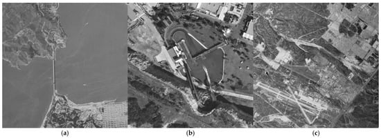
Figure 1.
Test single-channel (grayscale) images Frisco (a), Fr03 (b), and Diego (c), all 512 × 512 pixels.
Recall here that the HEIF coder, similarly to JPEG, is controlled by a QF varying from 1 (low quality of compressed images with large CR) to 100 (insignificant compression with very small losses). One specific feature of HEIF (here we used the version available at https://github.com/bigcat88/pillow_heif) is that the compression characteristics for pairs of neighbor values of QF (e.g., 3 and 4, 5 and 6) are practically identical [17]. The CR for HEIF (similarly to many other compression techniques) not only depends on the QS, but also on the image complexity and noise properties. To demonstrate this, consider the data in Table 1.

Table 1.
Compression ratio for the Frisco and Diego images for different QF and .
As expected, the CR increased when the QF was reduced. As also expected, the CR for the simple structure image was larger than the CR for the complex structure image for the same QF and . Quite small CR values (smaller than 3) were observed for both images for QF ≥ 59, where it was possible to note near-lossy compression. Meanwhile, there were two interesting observations. First, the CR decreased if the increased for a large QF (e.g., QF = 79); for a small QF, the CR for a larger was larger or practically the same (see data for QF = 9). Second, there was an interval of QF values (19–39) where the CR increased rapidly when the QF decreased, and this interval contained the QFOOP for the considered values of . Recall that the noise-filtering effect due to lossy compression is associated with the appearance of considerably more zero-valued DCT coefficients after quantization, and then the CR becomes significantly larger.
Figure 2 presents the dependences of the MSE calculated between the compressed and true images on the CR for two test images and two values of , 25 and 196, for five coders. As can be observed, OOPs were observed for all five coders (including the advanced DCT-based coder ADCT [58]) for both noise variances for the test image Frisco as well as for three coders (including HEIF) for the test image Diego, contaminated by AWGN with .
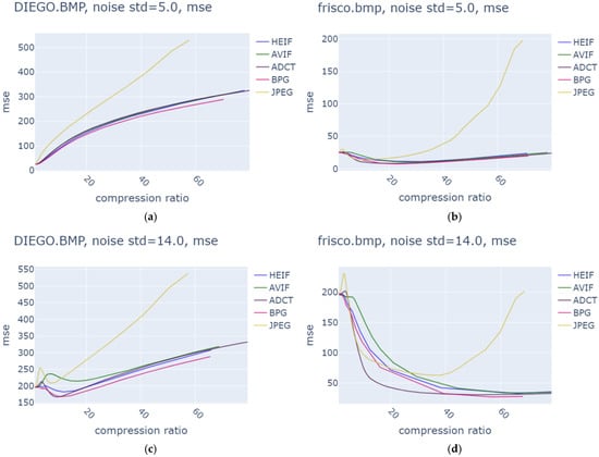
Figure 2.
Dependences of MSEtc (calculated between the true and compressed images) for images Diego (a,c) and Frisco (b,d) for (a,b) and (c,d) for five coders.
The plots presented in Figure 2 also reflect the main tendencies typical for the lossy compression of noisy images. First, the presence of the OOP is more probable for simpler structure images—compare the results in Figure 2a,b, where OOPs were absent for all coders for the test image Diego and present for all five coders for the test image Frisco. Second, the OOP presence is more likely for larger noise intensity—compare the results for the test image Diego for two values of the noise variance. Third, OOPs could be observed for approximately the same PCC values for different images contaminated by AWGN with the same variance—this follows from data presented in Table 1 (Notes column). Fourth, OOPs are “more obvious” for better coders–see data in Figure 2d where the MSEtc in the OOPs (minimal values of MSEtc) was smaller for modern coders than for JPEG (tc relates to metrics calculated between the compressed and true images). Fifth, if an OOP exists, then the CR in it will be quite large—from about 10 for complex structure images (Figure 2c) to 20–60 for simple structure images depending on the noise variance. One more positive feature of HEIF is that it performed better than AVIF (see data in Figure 2c,d) and approximately at the same level as the BPG coder. Also recall that HEIF was slightly faster than BPG.
The values of MSEtc were non-zero for all of the QF, test images, and noise variance values for HEIF (as well as other coders) for the plots in Figure 2. This means that there was some residual noise in the compressed image as well as some distortions of information content. A question is whether these residual noise and distortions can be additionally diminished by decompressed image post-filtering. Available results for the BPG coder have shown that this is possible [47,48], so why then should it not be possible for HEIF?
Note that the choice of a proper filter and its parameters depends on the properties of the noise to be removed. Therefore, similarly to [59], it was worth carrying out a statistical analysis for the mixture of residual noise and distortions for HEIF.
3. Distortion Statistical Analysis
In lossy image compression based on orthogonal transforms, distortions are due to the operation of transform coefficient quantization. This holds for both wavelet- and DCT-based coders. It has been found by several researchers for DCT-based [59], BPG [60], and JPEG [61] coders that:
- (1)
- The MSE of the introduced distortions increases (in most cases) monotonically if the PCC is changed to increase the CR [59,60];
- (2)
- Introduced distortions are “non-stationary”, in the sense that they are more intensive for the so-called active image areas (textures, neighborhoods of sharp edges, and high-contrast small-sized objects) [59];
- (3)
- Due to this, the integral MSE is usually larger for complex structure images with a larger percentage of pixels that belong to locally active areas [60,61]; meanwhile, it is less likely to have a non-Gaussian (heavy-tailed) distribution of introduced errors for complex-structure images than for simple-structure ones;
- (4)
- There is a tendency to have heavier tails of introduced errors for a larger CR [59];
- (5)
- In the lossy compression of noisy images with possible post-filtering, it is worth considering not only the statistics of the introduced errors, but also the statistics of the residual noise and distortions [60];
- (6)
- From the post-filtering viewpoint, it is desirable to not only analyze the statistics of the residual noise and distortions, but also their spatial correlation, since the removal of spatially correlated noise is a more complex task than AWGN suppression, and the efficiency of spatially-correlated noise removal is usually less than AWGN suppression for the same noise variance [62].
The statistics and spatial correlation characteristics of distortions may also depend on the noise statistics and spatial correlation if one is dealing with spatially-correlated noise, but this question was out of the scope of our study. Furthermore, we did not consider the case of signal-dependent noise, assuming that either the noise was close to pure additive or that an image contaminated by signal-dependent noise had been converted before compression by a proper variance stabilizing transform to be contaminated by additive noise [41,56]. Thus, our goal here was to study the statistical characteristics of residual noise/distortions for images corrupted by AWGN and compressed by HEIF.
We considered the noise/distortion parameter arrays , for two test images for three values of QF and two values of the noise variance, namely, 25 and 100. QF values were chosen to (1) correspond to the OOP for the image Frisco, or to quality degradation for the image Diego (the smallest considered QF); (2) relate to the case when the MSEtc was still almost the same as σ2 (the largest considered QF); and (3) correspond to intermediate situations (intermediate values of QF).
To study the statistics of , for each case, we calculated the mean, variance, skewness, and kurtosis (note that joint analysis of these parameters allows for the rough analysis of data Gaussianity). In addition, D’Agostino’s statistical K-squared test was applied [63], which aims to gauge the compatibility of given data with the null hypothesis that the data are a realization of independent, identically distributed Gaussian random variables. This test exploits two parameters. The parameter Stat is determined as s2 + k2, where s is the z-score returned by the skewtest (test whether the skew is different from the normal distribution), and k is the z-score returned by the kurtosistest (test whether a dataset has normal kurtosis). The parameter P is a 2-sided Chi-squared probability for the hypothesis test. According to the recommendations in [63], we assumed that alpha = 0.05 was a statistically significant level.
The obtained data are presented in Table 2. In addition to the aforementioned statistical parameters, we present the CR values useful for further analysis. The conclusions that can be drawn are as follows:
Table 2.
Statistics of the introduced distortions.
- (1)
- There were cases when , had a Gaussian distribution; this happened for the complex structure image Diego when the QF was large enough and the CR was quite small, and also took place for the test image Frisco when the CR was quite small;
- (2)
- On the contrary, , became non-Gaussian when the QF decreased and, respectively, the CR increased; the conclusions in items 1 and 2 were confirmed by both the analysis of kurtosis and D’Agostino’s K-squared test;
- (3)
- Mean and skewness of , were both close to zero;
- (4)
- For the same σ2, the variance of , was within wide limits; this ranged from 11 to 34 for σ2 = 25 and from 24 to 108 for σ2 = 100, where the minimal values corresponded to the OOP observed for the test image Frisco, and the maximal values related to the small QF for the test image Diego, for which the OOP was absent. This means that the variance can be either slightly larger than σ2 or several times smaller than σ2, which could be problematic in terms of setting the filter parameters correctly.
Let us also visualize , using the preliminary transformation Our goal here is to check whether we have something like white noise or the structure of , , which is more complex. Figure 3 shows , for QF = 50, σ2 = 100, for two test images. It was interesting to see that fluctuations in homogeneous regions of the test image Frisco were considerably less intensive compared with the fluctuations in locally active areas of this image as well as for practically the entire image of Diego. This was due to the noise-filtering effect, which appeared more in homogeneous image regions. Meanwhile, it is also possible to state that some “structures” were present in , due to the presence of some structures (objects, textures, edges) in the information component of the images subject to lossy compression.
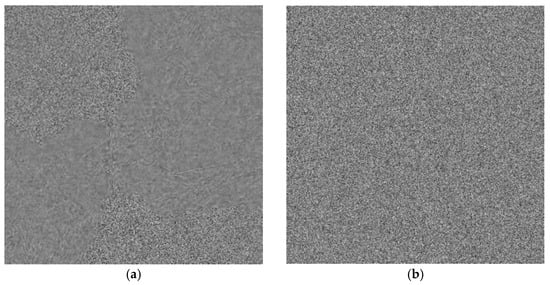
Figure 3.
Visualized , for the test images Frisco (a) and Diego (b) corrupted by AWGN with σ2 = 100 compressed by HEIF with QF = 50.
As a result, we cannot expect that positive features of known denoising techniques can be realized for the considered application to the full extent since they are designed to suppress , , which is obviously not exactly additive white Gaussian noise. However, it is possible to hope that some positive effects due to post-filtering can be achieved.
4. Post-Filtering Opportunities and Results
4.1. Post-Filtering Opportunities
Thus, we have to remove noise that has a probability density function (pdf) close to Gaussian (with possibly heavier tails), is almost white, and has an approximately known variance (MSE of residual noise and distortions that can be either slightly smaller or larger than the variance of the noise σ2 in the original image). Although there has been a huge number of image denoising techniques designed thus far (see survey papers [64,65,66] and references therein), our intention here was not to find the best filter for our application. Instead, our aim was to approximately estimate the potential of post-filtering and identify the main tendencies. Because of this, we decided to consider the famous block matching 3-dimensional (BM3D) filter [52,67], which is based on finding similar patches and using Haar and discrete cosine transforms for 3D denoising of the formed sets of similar blocks.
This filter has the following positive features that are useful for the considered application. First, the BM3D filter has a preset parameter β used for the threshold T setting as βσ. By changing β, it is possible to slightly vary the filter properties—a larger β leads to better noise suppression at the expense of worse edge/detail/texture preservation. In our case, this property can be useful to understand how the optimal or quasi-optimal threshold can be adjusted depending on the original σ2, and possibly some other information on the image at hand to be compressed. Second, a filter is quite insensitive if the noise pdf is not exactly Gaussian or not exactly white. This property is also important for the considered application. Third, the BM3D filter is one of the best filters in the sense of AWGN suppression, and its performance is comparable to that of neural network-based filters [68] (neural network-based filters mostly demonstrate better performance for unrealistically large values of σ).
4.2. Post-Filtering Performance Analysis
Filter performance is usually characterized by the output peak signal-to-noise ratio or its increase compared with the PSNR of the original noisy images [67]. Meanwhile, it has become popular to also analyze the visual quality metrics or their improvement due to filtering [69]. Below, we consider the metrics PSNR-HVS-M [32] and FSIM [70], which are among the best for characterizing denoising efficiency and the visual quality of images in general [68,69]. Recall here that we considered grayscale images, and hence not all visual quality metrics (mainly intended on characterizing the color image quality) could be applied. PSNR-HVS-M is expressed in dB and larger values correspond to a better visual quality. FSIM varies between 0 and 1, and larger values relate to better quality.
Post-filtering can be useful only under certain conditions (i.e., if it is efficient enough and if the provided CR is appropriately large). Because of this, we did not consider a QF > 51, for which the provided CR was small (see data in Table 1). Meanwhile, we also did not analyze a QF < 23, since it was expected that the filtering efficiency would be low [49]. In other words, we studied the behavior of post-filtering efficiency for the neighborhood of the optimal operation point (if it existed, see data in Table 2) and for a QF that produced a smaller CR than in the OOP. Namely, the interval of QF analysis was from 23 to 51.
Some preliminary results are presented in Table 3 for σ2 = 50. The optimal values for βopt, which provide the maximal output PSNR, are given, and the produced PSNR-HVS-M values are also presented. Recall here that the input PSNR was equal to 31.12 dB and the output PSNR for the BM3D filter applied to an uncompressed noisy image was equal to 39.45 dB for the image Frisco and 33.72 dB for the image Fr03. As seen, filtering was more efficient for the simpler structure image Frisco. For the complex structure image Fr03, the PSNR improvement was only 2.6 dB.
Table 3.
Post-filtering performance characteristics, σ2 = 50.
Analysis of the data in Table 3 allowed us to draw the following conclusions:
- (1)
- If the QF decreases (i.e., the CR increases and the noise-filtering effect of lossy compression becomes larger), the PSNR and PSNR-HVS for post-filtering decrease and the optimal β is also reduced; this means that the positive effect of post-filtering becomes smaller if the QF increases, and in fact, post-filtering for a small QF becomes useless;
- (2)
- There are QF values for which post-filtering is expedient; for example, for QF = 41, the values of PSNRtc for the compressed images were equal to 34.74 dB for Frisco and 30.38 dB for Fr03, respectively, while the PSNR values after post-filtering were equal to 39.03 dB for Frisco and 32.48 dB for Fr03, respectively;
- (3)
- Certainly, post-filtering is less efficient for complex structure images, and this property is in good agreement with the general denoising properties [51,55,69];
- (4)
- The PSNR-HVS-M metric demonstrated the same properties and confirmed the conclusions based on the PSNR analysis;
- (5)
- A reduction in βopt takes place if the QF decreases; this means that, in fact, the MSEtc might be reduced compared with σ2, and one needs to set a smaller threshold to make the filter perform in a quasi-optimal manner.
It is possible to represent the obtained data as surfaces depending on QF and β. Two examples are presented in Figure 4.
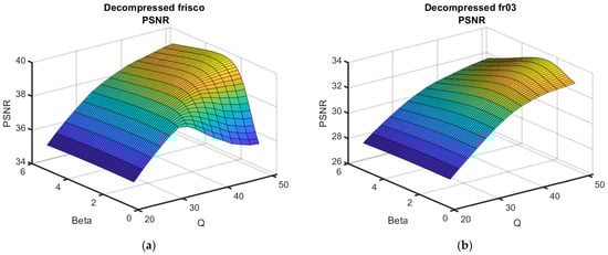
Figure 4.
Dependences of the output metrics on QF and β for two test images and three metrics, σ2 = 50. Plots of PSNR (a,b), PSNR-HVS (c,d) and FSIM (e,f) for the test images Frisco (a,c,e) and Fr03 (b,d,f).
As can be seen, the surfaces are smooth, and the maxima in the neighborhood of the optimal β are not “obvious” (i.e., for β, which slightly differed from βopt, the performance was practically the same as for βopt). This means that errors in setting β do not considerably influence the post-filtering efficiency. Meanwhile, the reduction in the metric output values with QF decreasing was not rapid for QF = 40, but the reduction speed increased for a smaller QF.
Let us now see what happens for other values of noise variance. The data obtained for σ2 = 100 are given in Table 4.
Table 4.
Post-filtering performance characteristics, σ2 = 100.
Recall that the input PSNR in this case was equal to 28.12 dB and the output PSNR for the BM3D filter applied to the uncompressed noisy image was 37.66 dB for the image Frisco and 31.71 dB for the image Fr03. Thus, filtering was again more efficient for the simpler structure image Frisco. For the image Fr03, the PSNR improvement was equal to 3.6 dB.
An analysis of the data in Table 4 allowed us to draw conclusions similar to the previous case of σ2 = 50:
- (1)
- If the QF is reduced (which corresponds to an increase in CR), the PSNR and PSNR-HVS for the post-filtered images decrease, and the optimal β also decreases; in other words, the positive effect of post-filtering becomes smaller, and starting from a certain QS, post-filtering becomes useless;
- (2)
- At the same time, there exist QF values for which the use of post-filtering is reasonable; for example, for QF = 39, the values of PSNRtc for the compressed images were equal to 28.66 dB for Frisco and 28.11 dB for Fr03, respectively. In turn, the PSNR values after post-filtering were equal to 37.36 dB for Frisco and 30.92 dB for Fr03, respectively;
- (3)
- Post-filtering is less efficient for complex structure images; for any QF, the output PSNRs were significantly smaller for test image Fr03 than for test image Frisco;
- (4)
- The PSNR-HVS-M metric showed the same dependencies;
- (5)
- A reduction in βopt is observed if the QF decreases; thus, one needs to set a smaller threshold to provide the filter operation in a quasi-optimal manner.
The functions of the metrics on QF and β are represented in Figure 5.
Figure 5.
Dependences of the output metrics on QF and β for two test images and three metrics, σ2 = 100. Plots of PSNR (a,b), PSNR-HVS (c,d) and FSIM (e,f) for the test images Frisco (a,c,e) and Fr03 (b,d,f).
As seen, the surfaces are again quite smooth; however, the maxima in the neighborhood of optimal β have become more “obvious” compared with the case of σ2 = 50 (Figure 4); nevertheless, for β, while it slightly differed from βopt, its performance was almost the same as for βopt. Thus, the post-filtering efficiency remained high for β within the limits of 2.0 to 2.5. Again, the reduction in metric output values with a decrease in QF was not rapid for QF = 36, while the reduction speed increased for a smaller QF.
Consider now the case of σ2 = 200. The obtained data are shown in Table 5.
Table 5.
Post-filtering performance characteristics, σ2 = 200.
The analysis of the data in Table 5 resulted in the following conclusions:
- (1)
- If the QF is reduced (i.e., the CR increases), both the PSNR and PSNR-HVS for the post-filtered images become worse, and the optimal β also reduces; this shows that the positive effect of post-filtering reduces, and starting from a QS around 23, post-filtering becomes useless;
- (2)
- There are QF values for which the post-filtering is beneficial; for example, for QF = 37, the values of PSNRtc for the compressed images were equal to 25.65 dB for Frisco and 25.39 dB for Fr03, respectively. In turn, the PSNR values after post-filtering were equal to 35.78 dB for Frisco and 29.41 dB for Fr03, respectively;
- (3)
- Again, the post-filtering was less efficient for the complex structure image Fr03 than for the test image Frisco;
- (4)
- The PSNR-HVS-M metric had similar dependencies;
- (5)
- A reduction in βopt is observed if the QF decreases; this means that one has to set a smaller threshold to provide the filter operating in a quasi-optimal manner.
- (6)
- The functions of the metrics on QF and β are represented in Figure 6.
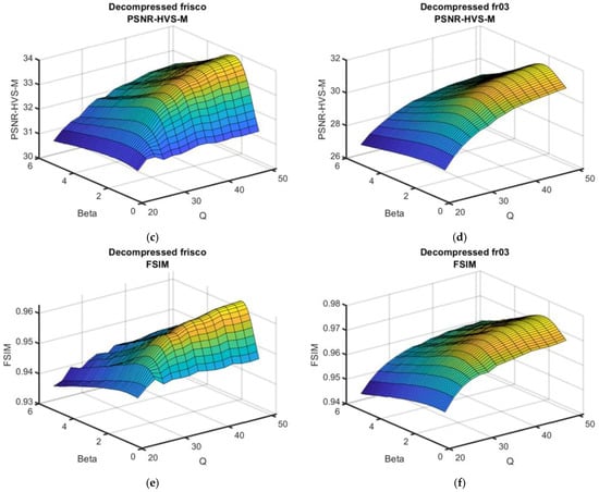 Figure 6. Dependences of the output metrics on QF and β for two test images and three metrics, σ2 = 200. Plots of PSNR (a,b), PSNR-HVS (c,d) and FSIM (e,f) for the test images Frisco (a,c,e) and Fr03 (b,d,f).
Their analysis showed that the surfaces had maxima in the neighborhood of optimal β; small deviations of β from βopt did not essentially reduce the performance. The post-filtering efficiency was high for a β of about 2.2. The reduction in the metric output values with QF decreasing was not rapid for QF ≥ 34 but the reduction speed increased for smaller QF.
The expedience of decompressed image post-filtering can be also studied in another way. Figure 7 presents the dependencies PSNRp pf = PSNRpf − PSNRtc (Q = 1) and ∆PSNRp tc = PSNRtc − PSNRtc (Q = 1) on the CR obtained by varying the QF and CR, respectively, for two test images and two noise variance values. Here, the PSNRpf was the PSNR calculated between the decompressed image post-filtered with the optimal β and the true image, and PSNRtc, as we recall, is the PSNR calculated between the compressed and true images.
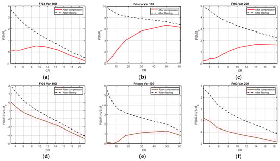
Figure 7.
Dependences of PSNRp pf (CR) and ∆PSNRp tc (CR) (a–c) and ∆PSNR-HVS-Mp pf (CR) and ∆PSNR-HVS-Mp tc (CR) (d–e) for the test images Fr03 (a,c,d,f) and Frisco (b,e) for σ2 = 100 (a,b,d,e) and σ2 = 200 (c,f).
Analysis of ∆PSNRp tc (Figure 7a–c) showed that in all three cases, OOPs existed (there was a maxima of ∆PSNRtc (CR)). Meanwhile, the maximal ∆PSNRp tc for the test image Fr03 (Figure 7a) was very small (about 0.5 dB). The maximal values of ∆PSNRp tc were larger for σ2 = 200 (σ2 is denoted as Var in the Figure title, see Figure 7c), and exceeded 6 dB for the test image Frisco (Figure 7b).
As seen, the PSNRp pf, in the considered limits of CR, was always larger than PSNRp tc. However, the difference between them decreased if the CR increased. In the neighborhood of the OOP (CR ≈ 10 in Figure 7a, CR ≈ 60 in Figure 7b, CR ≈ 14 in Figure 7c) and for a larger CR, the benefit due to post-filtering became negligible (about 0.5 dB and less) (i.e., post-filtering became practically useless).
Consider now the dependences PSNR-HVS-Mp pf = PSNR-HVS-Mpf − PSNR-HVS-Mtc (Q = 1) and PSNR-HVS-Mp tc = PSNR-HVS-Mtc − PSNR-HVS-Mtc (Q = 1) on the CR presented in Figure 7d–f. As seen, there were two cases when all PSNR-HVS-Mp tc were negative (Figure 7d,f) (i.e., there was no OOP for the test image Fr03). Meanwhile, there was an OOP according to the metric PSNR-HVS-M for the test image Frisco (Figure 7e), although the PSNR-HVS-Mp tc in this OOP was not large (slightly exceeded 1 dB).
As in the previous case of analysis, the PSNR-HVS-Mp pf was always larger than PSNR-HVS-Mp tc across the entire range of analyzed CR. However, the difference between PSNR-HVS-Mp pf and PSNR-HVS-Mp tc quickly reduced if the CR was increased (i.e., post-filtering became useless). In our opinion, it became practically useless for CR > 10 in Figure 7d, CR > 59 in Figure 7e, CR > 14 in Figure 7f) when the difference between the PSNR-HVS-Mp pf and PSNR-HVS-Mp tc was less than 1 dB (recall that a difference of less than 1 dB in the PSNR and PSNR-HVS-M of two images could hardly be noticed).
Nevertheless, in our opinion, the use of post-filtering could be reasonable for a smaller CR (e.g., for CR ≈ 8 (Figure 7a,d), CR ≈ 30 (Figure 7b,e), and CR ≈ 11 (Figure 7c,f), i.e., for a CR about 1.5 smaller than that one that corresponds to the OOP (if it exists)).
Based on the results presented above in this subsection and in Table 1 (as well as the results obtained for other test images and several noise variance values), it is possible to recommend setting the QF at 8–10 larger than the QF for the OOP. Keeping in mind the recommendations in [17], we offer the following recommendations on setting the QF, depending on the noise variance (supposed to be known in advance or accurately pre-estimated) for post-filtering to be reasonably applied. The recommended QF values are given in Table 6. As seen, the recommended QF decreases if the AWGN variance increases. In addition, we provide the ranges of PSNRpf, PSNR-HVS-Mpf, and CRpf. The parameter QFOOP as well as the ranges of PSNROOP, PSNR-HVS-MOOP, and CROOP are also presented.
Table 6.
The image compression parameters depending on the AWGN variance.
As seen, the values of PSNRpf were larger than the corresponding PSNROOP by about 1–3 dB, and the PSNR-HVS-Mpf values were sufficiently larger than the corresponding PSNR-HVS-MOOP for a noise variance smaller than 130. Meanwhile, the CR for image compression with post-filtering was 1.5–4 times smaller than for QFOOP, which is the price for better quality.
To ensure that the presented tendencies and recommendations were valid, we analyzed six additional images. Three of them were the optical test images Baboon (that has complex structure), Goldhill (middle-complexity structure), and Peppers (low complexity image). These images can be found at https://ponomarenko.info/agu.htm (accessed on 1 March 2025). Three other images were medical (Figure 8). These images have quite a simple structure since they contain rather large homogeneous image regions.
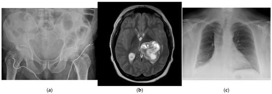
Figure 8.
Test images Med5 (a), Med7 (b), and Med8 (c) used in the additional experiments.
The results obtained for the six test images above-mentioned are shown in Table 7. We present the PSNR for the original noisy image, PSNRf for the filter output applied to the non-compressed image, PSNROOP for the OOP (according to data in Table 1), PSNRpf for the post-filtered images if the Q is set according to the recommendation in Table 6 and β is optimal, and the optimal β for each particular case.
Table 7.
Results for the additional test images.
The first conclusion that can be drawn from the comparison of data in Table 6 and Table 7 is that the PSNROOP and PSNRpf given in Table 7 were within the corresponding limits presented in Table 6. It can be clearly seen that the PSNROOP was always by about 3 dB smaller than the PSNRf (i.e., the noise filtering due to lossy compression was considerably less efficient than the traditional filtering applied to the uncompressed image). A comparison of the PSNROOP and PSNRpf for the same image and the same noise variance in Table 7 demonstrated that PSNRpf was 0.9–2.1 dB larger than the PSNROOP, where the largest benefit for the proposed approach was observed for simple structure images contaminated by intensive noise. The second conclusion is that the optimal β was in the range of 2.1 to 3.0, where the recommendation to set β ≈ 2.3 can be given for practice. Finally, the obtained data showed that: (1) the proposed approach is quite general and applicable to images of different origin; and (2) the results depend more on the image complexity than on the image origin domain.
Let us present some compression results. Figure 9a shows the noisy image Frisco, σ2 = 100. The image compressed by HEIF with QF = 25 (in the OOP) is presented in Figure 9b, while the same image compressed by HEIF with QF = 36 and post-filtered is shown in Figure 9c. As seen, noise in the homogeneous image regions was better suppressed while the edges and details were sharper (compare images in Figure 9c,b). The trade-off for this improvement was a lower level of CR. Figure 9d presents the noisy image Diego, σ2 = 100. Noise was only visible in small homogeneous regions. The compressed image (QF = 25) is shown in Figure 9e, and the image compressed by HEIF with QF = 36 and post-filtered is given in Figure 9f. Noise in the homogeneous parts was suppressed for both output images, but the edges and details were less smeared for the post-filtered image (Figure 9e).
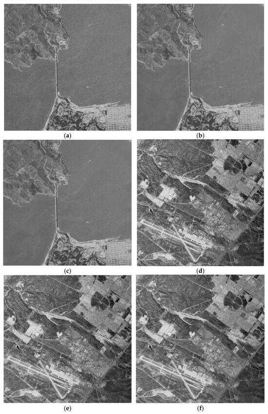
Figure 9.
Noisy image Frisco (a), the results of its compression in the OOP by HEIF (b), compressed with QF = 36 and post-filtered with the optimal β after decompression (c), noisy image Diego (d), the results of its compression in the OOP by HEIF (e), compressed with QF = 36 and post-filtered with the optimal β after decompression (f).
5. Discussion
In the sections above, we considered the simplest possible model of AWGN that contaminates a single component (grayscale) image. A question that arose is what are the differences that can be met in practice? Note that one can deal with an image corrupted by signal-dependent noise. Then, two ways are possible. One can follow the quite standard approach described in our paper [17] (i.e., apply a proper VST to convert the original image corrupted by signal-dependent noise to the image contaminated by pure additive noise). After this, the image should be compressed with QF, as recommended in Section 4.2, and stored or passed via the communication line. At the decompression and post-processing stage, just standard decompression by HEIF is carried out; after this, post-filtering is applied, and then inverse VST is performed. Within this procedure, the following is supposed: (1) the parameters of signal-dependent noise are a priori known or pre-estimated with high accuracy; (2) a proper variance-stabilizing transform exists and allows for the variance of pure additive noise to be determined; and (3) a priori information for carrying out inverse VST is available at the decompression stage (e.g., this information is passed as auxiliary data together with the compressed image in header). Another method is to study the application of HEIF to images corrupted by signal-dependent noise without VST, with proper recommendations. However, this method presumes additional investigations that need to be carried out.
Second, what does one do if the image to be compressed is multichannel? Currently, we are not ready to answer this question precisely. However, several analogies and preliminary solutions can be found. Note that a variety of possible situations is possible. It can be that a multichannel image contains one or two component images that are corrupted by the noise while other components are practically noise-free. Then, a noisy component image can be compressed separately, as described above, while other component images can be compressed (without post-filtering) separately or jointly, according to the approaches typical for the compression of noise-free multichannel images [7]. However, to the best of our knowledge, there have been no attempts to apply HEIF for the compression of multispectral or hyperspectral data.
If all or a large group of component images are noisy, then the approach described in [42] seems reasonable, as it presumes the use of proper VST for all component images and their joint compression (note that joint compression usually produces an approximately twice larger CR than component-wise compression for the same quality of compressed data). However, such an approach using HEIF as the basis needs additional studies.
An important item is to understand (predict) whether an OOP exists or not for HEIF. Currently, we do not know of such studies. However, since it has been shown for the BPG coder that such a prediction is possible [38], and the BPG and HEIF coders have similar performance characteristics [17], then it is reasonable to expect that the prediction of the existence of an OOP for HEIF is also possible.
In other words, there are many options in which to study the applicability of HEIF for the compression of remote sensing images, both single- and multichannel.
Finally, a future direction could focus on whether or not the compression of noisy images with post-filtering can influence the image classification [11], feature selection [71], image segmentation and edge detection [72], and object recognition [18]. For example, the National Research Foundation of Ukraine (https://nrfu.org.ua/en/, accessed on 1 March 2025) is interested in such studies within Project No. 2023. 04/0039 “Geospatial monitoring system for the war impact on the agriculture of Ukraine based on satellite data” (2024–2025).
In this sense, our recent studies [18] have shown the following. For quite a large range of CR variation, lossy compression and noise do not lead to a significant reduction in object recognition accuracy if modern neural networks (especially those in the YOLO (You Only Look Once) family [73]) are applied. Our preliminary results show that the use of post-filtering for the classification of compressed noisy images with visible noise allows for an increase in the total accuracy of correct classification by about 2% compared with the classification of noisy images compressed in the OOP. However, a neural network that carries out classification needs to be trained for post-filtered compressed noisy images.
6. Conclusions and Future Work
Our paper concerns the lossy compression of single-channel noisy images with the use of post-filtering after decompression to improve the image quality for the HEIF coder. This approach was compared with image compression in the optimal operation point if it existed, or for similar values of quality factor. It was shown that a positive effect of post-filtering exists for images of different complexity as well as different intensities of the noise. However, this positive effect varies: it can be large if a compressed image has a simple structure and the noise intensity is quite large and if the CR for a given QF is considerably smaller than the QF for the OOP. An opposite situation takes place if a given QF is quite close to the QF in the OOP. Because of this, we recommend reaching the compromise solutions presented in Table 6 depending on the noise variance for an 8-bit representation of data. This allows compression to be carried out with further post-filtering after decompression in fully automatic mode (this is important for practice). The output PSNR and PSNR-HVS-M were in this case considerably better than the PSNR and PSNR-HVS-M in the OOP, but the attained CR was 1.5–2 times smaller than for the QF that corresponded to the OOP.
There are many unsolved problems for HEIF. For example, it is desirable to carry out studies for cases of signal-dependent noise, multichannel images, and the classification of RS, CV, and medical data. The problem is that the variety of noise properties in multichannel images of different origin is so immense that we do not expect general solutions. At the same time, prominent solutions for particular situations can be achieved by the 3D compression of all components jointly or components properly combined in groups [41].
Author Contributions
Conceptualization, A.S. (Andrii Shelestov), V.G. and B.V.; Methodology, V.L., A.S. (Anatoliy Sachenko) and V.G.; Software, V.R. and S.K.; Validation, S.K., A.S. (Anatoliy Sachenko), and V.R.; Formal analysis, B.V. and V.L.; Investigation, A.S. (Andrii Shelestov); Writing—original draft preparation, V.L. and A.S. (Anatoliy Sachenko); Writing—review and editing, B.V., V.G. and A.S. (Andrii Shelestov); Visualization, S.K. and V.R.; Supervision, V.L. and B.V. All authors have read and agreed to the published version of the manuscript.
Funding
This research received no external funding.
Institutional Review Board Statement
Not applicable.
Informed Consent Statement
Not applicable.
Data Availability Statement
The original contributions presented in this study are included in the article. Further inquiries can be directed to the corresponding author.
Conflicts of Interest
The authors declare no conflicts of interest.
Abbreviations
The following abbreviations are used in this manuscript:
| OOP | Optimal operation point |
| CV | Computer vision |
| RS | Remote sensing |
| MD | Medical diagnostics |
| CR | Compression ratio |
| QF | Quality factor |
| DCT | Discrete cosine transform |
References
- Gandor, T.; Nalepa, J. First Gradually, Then Suddenly: Understanding the Impact of Image Compression on Object Detection Using Deep Learning. Sensors 2022, 22, 1104. [Google Scholar] [CrossRef] [PubMed]
- Kussul, N.; Lavreniuk, M.; Kolotii, A.; Skakun, S.; Rakoid, O.; Shumilo, L. A workflow for Sustainable Development Goals indicators assessment based on high-resolution satellite data. Int. J. Digit. Earth 2020, 13, 309–321. [Google Scholar] [CrossRef]
- Flint, A.C. Determining Optimal Medical Image Compression: Psychometric and Image Distortion Analysis. BMC Med. Imaging 2012, 12, 24. [Google Scholar] [CrossRef] [PubMed]
- Khorram, S.; van der Wiele, C.F.; Koch, F.H.; Nelson, S.A.C.; Potts, M.D. Future Trends in Remote Sensing. In Principles of Applied Remote Sensing; Springer International Publishing: Cham, Switzerland, 2016; pp. 277–285. ISBN 978-3-319-22559-3. [Google Scholar]
- Mallet, C. Multitemporal Earth Observation Image Analysis: Remote Sensing Image Sequences, 1st ed.; ISTE Invoiced Series; John Wiley & Sons, Incorporated: Newark, NJ, USA, 2024; ISBN 978-1-78945-176-4. [Google Scholar]
- Chow, K.; Tzamarias, D.E.O.; Blanes, I.; Serra-Sagristà, J. Using Predictive and Differential Methods with K2-Raster Compact Data Structure for Hyperspectral Image Lossless Compression. Remote Sens. 2019, 11, 2461. [Google Scholar] [CrossRef]
- Guo, L.; Zhou, D.; Zhou, J.; Kimura, S.; Goto, S. Lossy Compression for Embedded Computer Vision Systems. IEEE Access 2018, 6, 39385–39397. [Google Scholar] [CrossRef]
- Braunschweig, R.; Kaden, I.; Schwarzer, J.; Sprengel, C.; Klose, K. Image Data Compression in Diagnostic Imaging: International Literature Review and Workflow Recommendation. Rofo 2009, 181, 629–636. [Google Scholar] [CrossRef] [PubMed]
- Christophe, E. Hyperspectral Data Compression Tradeoff. In Optical Remote Sensing; Prasad, S., Bruce, L.M., Chanussot, J., Eds.; Springer: Berlin/Heidelberg, Germany, 2011; pp. 9–29. ISBN 978-3-642-14211-6. [Google Scholar]
- Liu, F.; Hernandez-Cabronero, M.; Sanchez, V.; Marcellin, M.W.; Bilgin, A. The Current Role of Image Compression Standards in Medical Imaging. Information 2017, 8, 131. [Google Scholar] [CrossRef] [PubMed]
- Yang, K.; Jiang, H. Optimized-SSIM Based Quantization in Optical Remote Sensing Image Compression. In Proceedings of the 2011 Sixth International Conference on Image and Graphics, Hefei, China, 12–15 August 2011; IEEE: New York, NY, USA, 2011; pp. 117–122. [Google Scholar]
- Bondžulić, B.; Stojanović, N.; Petrović, V.; Pavlović, B.; Miličević, Z. Efficient Prediction of the First Just Noticeable Difference Point for JPEG Compressed Images. Acta Polytech. Hung. 2021, 18, 201–220. [Google Scholar] [CrossRef]
- Yee, D.; Soltaninejad, S.; Hazarika, D.; Mbuyi, G.; Barnwal, R.; Basu, A. Medical Image Compression Based on Region of Interest Using Better Portable Graphics (BPG). In Proceedings of the 2017 IEEE International Conference on Systems, Man, and Cybernetics (SMC), Banff, AB, Canada, 5–8 October 2017; IEEE: Banff, AB, Canada, 2017; pp. 216–221. [Google Scholar]
- Blau, Y.; Michaeli, T. Rethinking Lossy Compression: The Rate-Distortion-Perception Tradeoff. In Proceedings of the International Conference on Machine Learning, Long Beach, CA, USA, 9–15 June 2019; PMLR. pp. 675–685. [Google Scholar]
- Li, F.; Abramov, S.; Dohtiev, I.; Lukin, V. Advantages and drawbacks of two-step approach to providing desired parameters in lossy image compression. Adv. Inf. Syst. 2024, 8, 57–63. [Google Scholar]
- Zemliachenko, A.; Lukin, V.; Ponomarenko, N.; Egiazarian, K.; Astola, J. Still Image/Video Frame Lossy Compression Providing a Desired Visual Quality. Multidimens. Syst. Signal Process. 2016, 27, 697–718. [Google Scholar] [CrossRef]
- Kryvenko, S.; Lukin, V.; Vozel, B. Lossy Compression of Single-channel Noisy Images by Modern Coders. Remote Sens. 2024, 16, 2093. [Google Scholar] [CrossRef]
- Radosavljević, M.; Brkljač, B.; Lugonja, P.; Crnojević, V.; Trpovski, Ž.; Xiong, Z.; Vukobratović, D. Lossy Compression of Multispectral Satellite Images with Application to Crop Thematic Mapping: A HEVC Comparative Study. Remote Sens. 2020, 12, 1590. [Google Scholar] [CrossRef]
- Lee, J.-S.; Pottier, E. Polarimetric Radar Imaging: From Basics to Applications; Optical Science and Engineering; CRC Press: Boca Raton, FL, USA, 2009; ISBN 978-1-4200-5497-2. [Google Scholar]
- Smolka, B.; Kusnik, D.; Radlak, K. On the Reduction of Mixed Gaussian and Impulsive Noise in Heavily Corrupted Color Images. Sci. Rep. 2023, 13, 21035. [Google Scholar] [CrossRef] [PubMed]
- Zhong, P.; Wang, R. Multiple-Spectral-Band CRFs for Denoising Junk Bands of Hyperspectral Imagery. IEEE Trans. Geosci. Remote Sens. 2013, 51, 2260–2275. [Google Scholar] [CrossRef]
- Abramova, V.; Abramov, S.; Abramov, K.; Vozel, B. Blind Evaluation of Noise Characteristics in Multichannel Images. In Information Technologies in the Design of Aerospace Engineering; Nechyporuk, M., Pavlikov, V., Krytskyi, D., Eds.; Studies in Systems, Decision and Control; Springer Nature: Cham, Switzerland, 2024; Volume 507, pp. 209–229. ISBN 978-3-031-43578-2. [Google Scholar]
- Wang, W.; Zhong, X.; Su, Z. On-Orbit Signal-to-Noise Ratio Test Method for Night-Light Camera in Luojia 1-01 Satellite Based on Time-Sequence Imagery. Sensors 2019, 19, 4077. [Google Scholar] [CrossRef]
- Ahmad, A.; Amira, K.; Mawardy, M.; Firdaus, S.; Yazid, M.; Rahman, A. Noise and Restoration of UAV Remote Sensing Images. Int. J. Adv. Comput. Sci. Appl. 2020, 11, 175–183. [Google Scholar] [CrossRef]
- Odegard, J.E.; Guo, H.; Burrus, C.S.; Baraniuk, R.G. Joint compression and Speckle Reduction of SAR Images Using Embedded Zero-tree Models. In Proceedings of the Workshop on Image and Multidimensional Signal Processing, Belize City, Belize, 3–6 March 1996; pp. 80–81. [Google Scholar]
- Wei, D.; Odegard, J.E.; Guo, H.; Lang, M.; Burrus, C.S. Simultaneous noise reduction and SAR image data compression using best wavelet packet basis. In Proceedings of the IEEE International Conference on Image Processing, Washington, DC, USA, 23–26 October 1995; pp. 200–203. [Google Scholar]
- Chang, S.G.; Yu, B.; Vetterli, M. Image Denoising via Lossy Compression and Wavelet Thresholding. In Proceedings of the International Conference on Image Processing, Santa Barbara, CA, USA, 26–29 October 1997; Volume 1, pp. 604–607. [Google Scholar]
- Al-Shaykh, O.K.; Mersereau, R.M. Lossy Compression of Noisy Images. IEEE Trans. Image Process. 1998, 7, 1641–1652. [Google Scholar] [CrossRef]
- Wallace, G. The JPEG Still Picture Compression Standard. Commun. ACM 1991, 34, 30–44. [Google Scholar] [CrossRef]
- Taubman, D.S.; Marcellin, M.W. JPEG2000: Image Compression Fundamentals, Standards, and Practice; Kluwer Academic Publishers: Boston, MA, USA, 2002; 779p. [Google Scholar]
- Ponomarenko, N.; Krivenko, S.; Lukin, V.; Egiazarian, K.; Astola, J.T. Lossy Compression of Noisy Images Based on Visual Quality: A Comprehensive Study. EURASIP J. Adv. Signal Process. 2010, 2010, 976436. [Google Scholar] [CrossRef][Green Version]
- Ponomarenko, N.; Silvestri, F.; Egiazarian, K.; Carli, M.; Astola, J.; Lukin, V. On Between-Coefficient Contrast Masking of DCT Basis Functions. In Proceedings of the Third International Workshop on Video Processing and Quality Metrics for Consumer Electronics, Scottsdale, AZ, USA, 25–26 January 2007. 4p. [Google Scholar]
- Wang, Z.; Simoncelli, E.P.; Bovik, A.C. Multiscale Structural Similarity for Image Quality Assessment. In Proceedings of the Thirty-Seventh Asilomar Conference on Signals, Systems & Computers, Pacific Grove, CA, USA, 9–12 November 2003; IEEE: Pacific Grove, CA, USA, 2003; pp. 1398–1402. [Google Scholar]
- Ziaei Nafchi, H.; Shahkolaei, A.; Hedjam, R.; Cheriet, M. Mean Deviation Similarity Index: Efficient and Reliable Full-Reference Image Quality Evaluator. IEEE Access 2016, 4, 5579–5590. [Google Scholar] [CrossRef]
- Ponomarenko, N.; Zriakhov, M.; Lukin, V.V.; Astola, J.T.; Egiazarian, K.O. Estimation of Accessible Quality in Noisy Image Compression. In Proceedings of the 2006 14th European Signal Processing Conference, Florence, Italy, 4–8 September 2006; pp. 1–4. [Google Scholar]
- Zemliachenko, A.N.; Abramov, S.K.; Lukin, V.V.; Vozel, B.; Chehdi, K. Lossy Compression of Noisy Remote Sensing Images with Prediction of Optimal Operation Point Existence and Parameters. J. Appl. Remote Sens. 2015, 9, 095066. [Google Scholar] [CrossRef]
- Kovalenko, B.; Lukin, V.; Kryvenko, S.; Naumenko, V.; Vozel, B. BPG-Based Automatic Lossy Compression of Noisy Images with the Prediction of an Optimal Operation Existence and Its Parameters. Appl. Sci. 2022, 12, 7555. [Google Scholar] [CrossRef]
- Tran, K.P.; He, Z. Computational Techniques for Smart Manufacturing in Industry 5.0: Methods and Applications; CRC Press: Boca Raton, FL, USA, 2025; ISBN 978-1-04-022820-3. [Google Scholar]
- BPG Image Format. Available online: https://bellard.org/bpg/ (accessed on 14 November 2024).
- Barman, N.; Martini, M.G. An Evaluation of the Next-Generation Image Coding Standard AVIF. In Proceedings of the 2020 Twelfth International Conference on Quality of Multimedia Experience (QoMEX), Athlone, Ireland, 26–28 May 2020; IEEE: Athlone, Ireland, 2020; pp. 1–4. [Google Scholar]
- Zemliachenko, A.; Kozhemiakin, R.; Uss, M.; Abramov, S.; Ponomarenko, N.; Lukin, V.; Vozel, B.; Chehdi, K. Lossy compression of hyperspectral images based on noise parameters estimation and variance stabilizing transform. J. Appl. Remote Sens. 2014, 8, 25. [Google Scholar] [CrossRef]
- Colom, M.; Buades, A.; Morel, J.-M. Nonparametric Noise Estimation Method for Raw Images. J. Opt. Soc. Am. A 2014, 31, 863–871. [Google Scholar] [CrossRef]
- Uss, M.L. Maximum Likelihood Estimation of Spatially Correlated Signal-Dependent Noise in Hyperspectral Images. Opt. Eng. 2012, 51, 111712. [Google Scholar] [CrossRef]
- Sendur, L.; Selesnick, I.W. Bivariate shrinkage with local variance estimation. IEEE Signal Process. Lett. 2002, 9, 438–441. [Google Scholar] [CrossRef]
- Ponomarenko, N.N.; Lukin, V.V.; Zriakhov, M.S.; Kaarna, A.; Astola, J. Automatic Approaches to On-Land/On-Board Filtering and Lossy Compression of AVIRIS Images. In IGARSS 2008, Proceedings of the 2008 IEEE International Geoscience and Remote Sensing Symposium, Boston, MA, USA, 6–11 July 2008; IEEE: Boston, MA, USA, 2008; pp. III-254–III-257. [Google Scholar]
- Lukin, V. Processing of Multichannel Remote Sensing Data for Environment Monitoring. In GeoSpatial Visual Analytics; Amicis, R.D., Stojanovic, R., Conti, G., Eds.; NATO Science for Peace and Security Series C: Environmental Security; Springer: Dordrecht, The Netherlands, 2009; pp. 129–138. ISBN 978-90-481-2898-3. [Google Scholar]
- Kovalenko, B.; Rebrov, V.; Lukin, V. Analysis of the Potential Efficiency of Post-Filtering Noisy Images After Lossy Compression. Ukr. J. Remote Sens. 2023, 10, 11–16. [Google Scholar] [CrossRef]
- Rebrov, V.; Vozel, B.; Lukin, V. Post-Filtering of Lossy Compressed Noisy Images and Its Efficiency Prediction. Adv. Inf. Syst. 2024, 8, 39–45. [Google Scholar] [CrossRef]
- Wang, L.; Wang, C.; Huang, W.; Zhou, X. Image Deblocking Scheme for JPEG Compressed Images Using an Adaptive-Weighted Bilateral Filter. J. Inf. Process. Syst. 2016, 12, 631–643. [Google Scholar] [CrossRef]
- Ahsan, S.S.; Esmaeilzehi, A.; Ahmad, M.O. OODNet: A Deep Blind JPEG Image Compression Deblocking Network Using out-of-Distribution Detection. J. Vis. Commun. Image Represent. 2024, 104, 104302. [Google Scholar] [CrossRef]
- Pogrebnyak, O.; Lukin, V.V. Wiener Discrete Cosine Transform-Based Image Filtering. J. Electron. Imaging 2012, 21, 043020. [Google Scholar] [CrossRef]
- Dabov, K.; Foi, A.; Katkovnik, V.; Egiazarian, K. Image Denoising by Sparse 3-D Transform-Domain Collaborative Filtering. IEEE Trans. Image Process. 2007, 16, 2080–2095. [Google Scholar] [CrossRef]
- Pastuszak, G.; Abramowski, A. Algorithm and Architecture Design of the H.265/HEVC Intra Encoder. IEEE Trans. Circuits Syst. Video Technol. 2016, 26, 210–222. [Google Scholar] [CrossRef]
- Gonzalez, R.C.; Woods, R.E. Digital Image Processing; Prentice Hall: Upper Saddle River, NJ, USA, 2008; ISBN 978-0131687288. [Google Scholar]
- Chatterjee, P.; Milanfar, P. Is Denoising Dead? IEEE Trans. Image Process 2010, 19, 895–911. [Google Scholar] [CrossRef]
- Zhang, B.; Fadili, M.J.; Starck, J.-L. Multi-Scale Variance Stabilizing Transform for Multi-Dimensional Poisson Count Image Denoising. In Proceedings of the IEEE International Conference on Acoustics Speech and Signal Processing, Toulouse, France, 14–19 May 2006. 4p. [Google Scholar] [CrossRef]
- Zheng, H.; Liu, Q.; Kravchenko, I.I.; Zhang, X.; Huo, Y.; Valentine, J.G. Multichannel Meta-Imagers for Accelerating Machine Vision. Nat. Nanotechnol. 2024, 19, 471–478. [Google Scholar] [CrossRef] [PubMed]
- Ponomarenko, N.; Lukin, V.; Egiazarian, K.; Astola, J. ADCTC: Advanced DCT-Based Coder. In Proceedings of the 2008 International Workshop on Local and Non-Local Approximation in Image Processing, LNLA2008, Lausanne, Switzerland, 23–24 August 2008; p. 6. [Google Scholar]
- Abramova, V.; Lukin, V.; Abramov, S.; Abramov, K.; Bataeva, E. Analysis of Statistical and Spatial Spectral Characteristics of Distortions in Lossy Image Compression. In Proceedings of the 2022 IEEE 2nd Ukrainian Microwave Week (UkrMW), Kharkiv, Ukraine, 14–18 November 2022; IEEE: Kharkiv, Ukraine, 2022; pp. 644–649. [Google Scholar]
- Kovalenko, B.; Lukin, V.; Vozel, B. BPG-Based Lossy Compression of Three-Channel Noisy Images with Prediction of Optimal Operation Existence and Its Parameters. Remote Sens. 2023, 15, 1669. [Google Scholar] [CrossRef]
- Wang, Q.; Liu, P.; Zhang, L.; Cheng, F.; Qiu, J.; Zhang, X. Rate–Distortion Optimal Evolutionary Algorithm for JPEG Quantization with Multiple Rates. Knowl.-Based Syst. 2022, 244, 108500. [Google Scholar] [CrossRef]
- Rubel, O.; Lukin, V.; Egiazarian, K. Additive Spatially Correlated Noise Suppression by Robust Block Matching and Adaptive 3D Filtering (JIST-First). Electron. Imaging 2019, 2019, 60401-1–60401-11. [Google Scholar] [CrossRef]
- D’Agostino, R.B. Transformation to Normality of the Null Distribution of g1. Biometrika 1970, 57, 679–681. [Google Scholar] [CrossRef]
- Mary Mathew, I.; Akhilaraj, D.; Zacharias, J. A Survey on Image Denoising Techniques. In Proceedings of the 2023 International Conference on Control, Communication and Computing (ICCC), Thiruvananthapuram, India, 19 May 2023; IEEE: Thiruvananthapuram, India, 2023; pp. 1–6. [Google Scholar]
- Zhang, D.; Zhou, F.; Albu, F.; Wei, Y.; Yang, X.; Gu, Y.; Li, Q. An Overview of Self-Supervised Image Denoising. Res. Sq. 2024, 1–20. [Google Scholar] [CrossRef]
- Elad, M.; Kawar, B.; Vaksman, G. Image Denoising: The Deep Learning Revolution and Beyond—A Survey Paper. SIAM J. Imaging Sci. 2023, 16, 1594–1654. [Google Scholar] [CrossRef]
- Alnuaimy, A.N.H.; Jawad, A.M.; Abdulkareem, S.A.; Mustafa, F.M.; Ivanchenko, S.; Toliupa, S. BM3D Denoising Algorithms for Medical Image. In Proceedings of the 2024 35th Conference of Open Innovations Association (FRUCT), Tampere, Finland, 24 April 2024; IEEE: Tampere, Finland, 2024; pp. 135–141. [Google Scholar]
- Malik, J.; Kiranyaz, S.; Yamac, M.; Gabbouj, M. Bm3d Vs 2-Layer Onn. In Proceedings of the 2021 IEEE International Conference on Image Processing (ICIP), Anchorage, AK, USA, 19–22 September 2021; IEEE: Anchorage, AK, USA, 2021; pp. 1994–1998. [Google Scholar]
- Rubel, O.; Lukin, V.; Abramov, S.; Vozel, B.; Pogrebnyak, O.; Egiazarian, K. Is Texture Denoising Efficiency Predictable? Int. J. Patt. Recogn. Artif. Intell. 2018, 32, 1860005. [Google Scholar] [CrossRef]
- Zhang, L.; Zhang, L.; Mou, X.; Zhang, D. FSIM: A Feature Similarity Index for Image Quality Assessment. IEEE Trans. Image Process. 2011, 20, 2378–2386. [Google Scholar] [CrossRef] [PubMed]
- Perova, I.; Bodyanskiy, Y. Adaptive Human Machine Interaction Approach for Feature Selection-Extraction Task in Medical Data Mining. Int. J. Comput. 2018, 17, 113–119. [Google Scholar] [CrossRef]
- Zahorodnia, D.; Pigovsky, Y.; Bykovyy, P. Canny-Based Method of Image Contour Segmentation. Int. J. Comput. 2016, 15, 200–205. [Google Scholar] [CrossRef]
- Jocher, G.; Chaurasia, A.; Stoken, A.; Borovec, J.; NanoCode012; Kwon, Y.; Michael, K.; Tao, X.; Fang, J.; Imyhxy; et al. Ultralytics/Yolov5: V7.0—YOLOv5 SOTA Realtime Instance Segmentation. 2022. Available online: https://ui.adsabs.harvard.edu/abs/2022zndo...3908559J/abstract (accessed on 6 March 2025).
Disclaimer/Publisher’s Note: The statements, opinions and data contained in all publications are solely those of the individual author(s) and contributor(s) and not of MDPI and/or the editor(s). MDPI and/or the editor(s) disclaim responsibility for any injury to people or property resulting from any ideas, methods, instructions or products referred to in the content. |
© 2025 by the authors. Licensee MDPI, Basel, Switzerland. This article is an open access article distributed under the terms and conditions of the Creative Commons Attribution (CC BY) license (https://creativecommons.org/licenses/by/4.0/).