Innovative Approach Integrating Machine Learning Models for Coiled Tubing Fatigue Modeling

Abstract

Coiled tubing (CT) plays a pivotal role in oil and gas well intervention operations due to its advantages, such as flexibility, fast mobilization, safety, low cost, and its wide range of applications, including well intervention, cleaning, stimulation, fluid displacement, cementing, and drilling. However, CT is subject to fatigue and mechanical damage caused by repeated bending cycles, internal pressure, and environmental factors, which can lead to premature failure, high operational costs, and production downtime. With the development of CT properties and modes of application, traditional fatigue life prediction methods based on analytical models integrated in the tracking process showed, in some cases, an underestimate or overestimate of the actual fatigue life of CT, particularly when complex factors like welding type, corrosive environment, and high-pressure variation are involved. This study addresses this limitation by introducing a comprehensive machine learning-based approach to improve the accuracy of CT fatigue life prediction, using a dataset derived from both lab-scale and full-scale fatigue tests. We incorporated the impact of different parameters such as CT grades, wall thickness, CT diameter, internal pressure, and welding types. By using advanced machine learning techniques such as artificial neural networks (ANNs) and Gradient Boosting Regressor, we obtained a more precise estimation of the number of cycles to failure than traditional models. The results from our machine learning analysis demonstrated that CatBoost and XGBoost are the most suitable models for fatigue life prediction. These models exhibited high predictive accuracy, with R² values exceeding 0.94 on the test set, alongside relatively low error metrics (MSE, MAE and MAPE), indicating strong generalization capability. The results of this study show the importance of the integration of machine learning for CT fatigue life analysis and demonstrate its capacity to enhance prediction accuracy and reduce uncertainty. A detailed machine learning model is presented, emphasizing the capability to handle complex data and improve prediction under diverse operational conditions. This study contributes to more reliable CT management and safer, more cost-efficient well intervention operations.

1. Introduction

Coiled tubing (CT) is considered an important well intervention service due to its advantages such as flexibility compared to threaded joints for reaching downhole bottoms during various operations [1].

Since its introduction to the oil and gas industry, coiled tubing has been the subject of extensive research due to its reliability and performance in operations and service life, as well as its potential to prevent failures.

Coil tubing consists of a long tube spooled onto a reel, which is set on a CT unit. This tubing can be stripped from the reel and smoothly run in and out of the hole through an arch guide and injector, enabling a wide range of applications, including well kick-off, hole cleaning, production stimulation, cementing, fishing, and coiled tubing drilling.

Throughout its service life, CT encounters several challenges, including rupture, mechanical damage, and fatigue [2]. This can lead to failures and expensive costs related to string loss or recovery operations, and production cuts [3,4].

While running, CT is subject to three cycles of bending and straightening combined with other factors such as fluid type, pumping pressures, CT unit design, and material properties. Over time, this contributes to the fatigue of CT [5].

Since 1980, many research studies have been conducted to understand the fatigue behavior and mechanisms of CT by developing predictive models based on full-scale and lab-scale fatigue tests. It takes into account various data, including material properties, applied forces, bending stresses, internal pressure, environmental conditions, and metal defects [6,7,8].

The modeling approach relies on principles of accounting for cumulative fatigue damage through Miner’s rule, power-law damage, and the double linear damage rule [4]. Generally, the strain life method and the Manson–Coffin equation are the most useful equations for modeling low cycle fatigue, as the CT is subject to plastic deformation [9,10,11].

Fatigue damage refers to the amount of CT life consumed by each event. Based on the plasticity theory and the full-scale fatigue testing data, Tipton presented the Achilles CT fatigue model, which depends on the strain–life method and the Von Mises equation to calculate fatigue damage using the effective amplitude strain in strain–life curves. Additionally, it calculates diametrical changes in the CT’s diameter [12].

The other well-known model is Avakov’s model, which calculates fatigue damage using the equivalent uniaxial alternating strain equation and strain–life method in strain–life curves [13]. The authors of [14] presented a model of CT fatigue life based on the tri-axial strain state of the strain–life approach. An experimental test was conducted in parallel with FEA analysis to predict the fatigue life and integration with developed software [14]. Other CT fatigue modeling efforts were based on metal defects and crack propagation, and a good correlation and strong results were found [5,15,16].

The most popular computational software recognized in the oil and gas industry includes Halliburton, CTES, Cycle, COILLIFE, Halliburton, and MEDCO, among others [12,17].

Despite the implementation of these processes that have served well in this industry, CT has frequently experienced fatigue failures prior to achieving the fatigue life yield predicted by those softwares. These occurrences have prompted ongoing investigations by researchers into the accuracy of different factors, addressing the complexity of data and integration, such as corrosive environments [18], surface anomalies [15,19], and slip damage [20]. Consequently, to address this issue with the advancements in the development of new CT grades and the challenges posed by well geometry, numerous experimental lab-scale and full-scale fatigue assessments have been conducted, updating the methodology and tracking process to improve CT fatigue life estimation [11,21,22,23,24,25].

In recent years, artificial intelligence (AI) and machine learning (ML) techniques have gained traction in tackling complex and non-linear data, including material fatigue behavior [5,26]. With their ability to analyze large and complicated datasets, machine learning has emerged as a sophisticated tool that reduces the uncertainty present in traditional methods [27].

Unlike traditional modeling, machine learning and artificial neural network (ANN) techniques, such as back propagation algorithms with time series methods, have rarely been used. Studies from the literature [28] have used CT sample fatigue tests [29] and applied a BP neural network, showing promising results for predicting the number of cycles, even with a small amount of data and excluding the factor of welding type. Additionally, regression modeling along with experimental fatigue tests of non-welded CT specimens has demonstrated a strong correlation between CT deformation and fatigue progression [30].

Through the studies, we identified several experimental coiled tubing fatigue tests that were published, including CT fatigue lab tests and CT full-scale fatigue tests. These fatigue testing projects and studies aimed to improve the fatigue life of CT by studying different grades of material, various weld processes, and the role of internal pressure in CT durability (N is the number of cycles, where one cycle indicates the bending and straightening of the CT segment).

However, most of those studies focused on one parameter, such as pressure, the grade, metal defect, etc., and used traditional modeling methods to predict the number of cycles N [20,28,31].

According to the literature and to the authors’ knowledge, there is a significant lack of use of machine learning techniques. In this regard, the current study attempted to address this gap by applying advanced machine learning techniques.

In the first step, we collected a large set of fatigue test data from different published experimental tests to obtain highly accurate modeling results. Then, we applied ML and ANN techniques. The dataset includes more than 350 tests covering various grades, wall thickness, CT diameters, pressure, and welding types. The dataset includes both lab- and full-scale tests to maximize accuracy in predicting the fatigue life of coiled tubing [13,14,21,23,29,32,33,34,35,36].

In addition, this paper presents an approach that utilizes multiple machine learning approaches, such as ANNs and gradient-boosting techniques, and employs datasets to accurately predict the number of cycles to failure (N) while comparing different machine learning techniques for evaluation and recommendation.

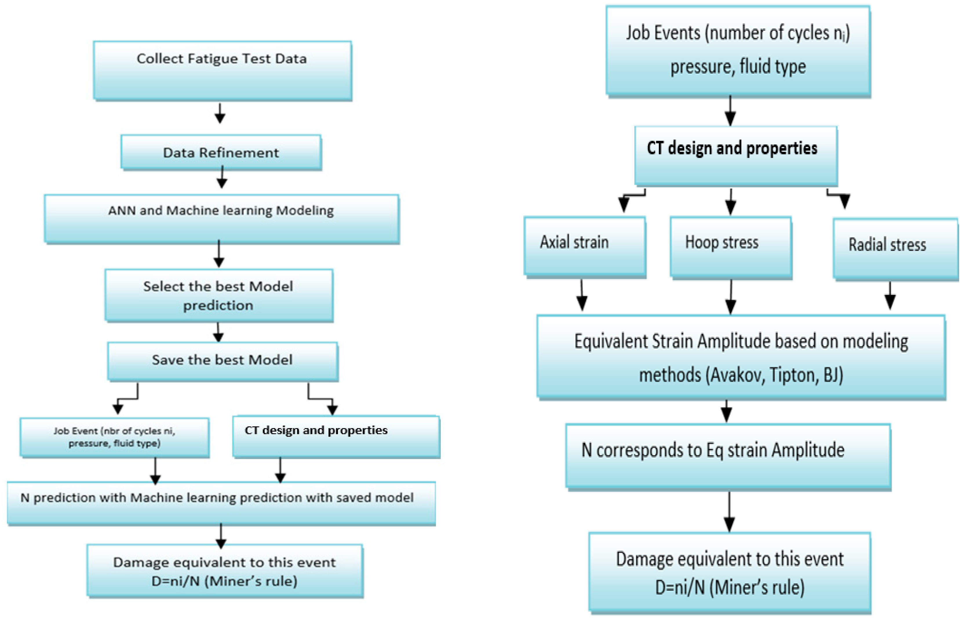
2. Data and Methodology

Introduction

In the literature, machine learning (ML) techniques are widely used to model the fatigue life of materials [6]. These advantages come from its simplicity and efficacy in treating a large set of non-linear and random data, including experimental testing data and field data.

This subject is divided into two categories, deterministic and non-deterministic approaches, and is based on the result type, as shown in Figure 1 [6], In this work, we will use the deterministic approach because the outcome of the modeling is the CT fatigue life in terms of the number of cycles (N).

In Figure 2, the methodology proposed in this work is compared to the conventional modeling for coiled tubing fatigue and tracking processes.

3. Data Description and Preprocessing

Dataset Overview

The dataset used in this study contains most of the parameters that impact the fatigue life of coiled tubing used in lab- and full-scale tests. The full-scale fatigue test aims to simulate the actual state in full scale from the coiled tubing reel through the arch. Then, the straightener is inserted into the well, as shown in Figure 3. Due to its complexity, the required equipment and cost, only a small number of such tests have been conducted. Generally, only service companies have performed this test to enhance their tracking processes and ensure successful service delivery [33,34,35]. Unlike the full-scale fatigue test, the lab-scale test contains a simplified design that uses a segment of CT (+/− 6-10 feet) fixed on one side in the testing machine, as shown in Figure 4, while bending cycles are applied from the other side until failure [30,37,38].

The dataset is as follows:

• Grade: Integer representing the CT material grade.
• CT Diameter: A continuous variable representing the outside diameter of the CT.
• Wall thickness: A continuous variable representing the thickness of coiled tube.
• Welding type: A categorical variable with different welding types used between CT segments (bias, manual, orbital, etc.).
• Radius: A continuous variable representing the bending radius of the testing machine.
• Pressure: Integer indicating the applied pressure while testing.
• N cycle: The target variable representing the number of cycles before failure.

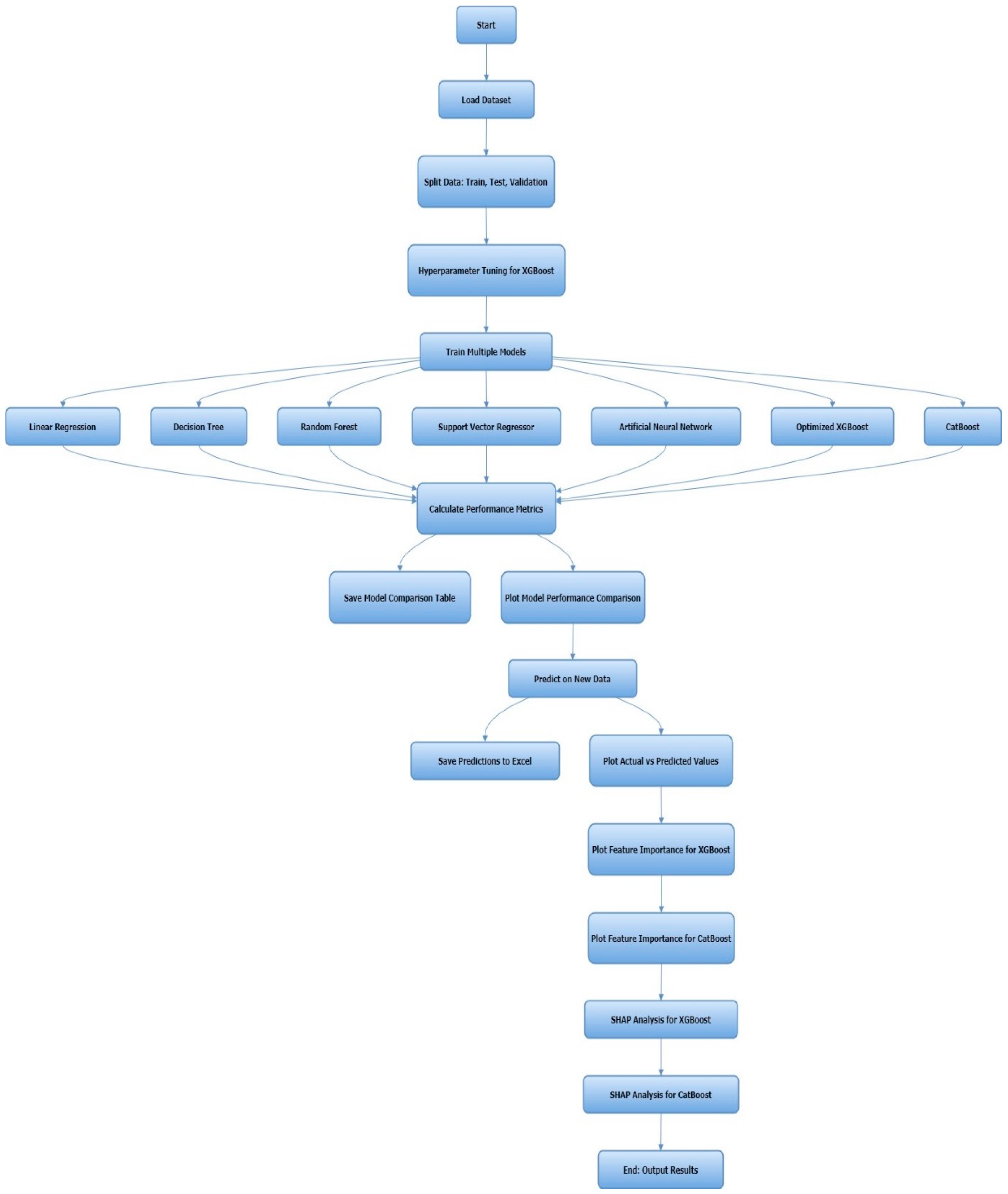
4. Data Processing and Algorithms

Using Python (Version 3.11.5) as a programming language to apply machine learning models, the dataset underwent several processing steps, starting from one-hot encoding to transform the categorical variable weld type into numerical features. Next, the dataset was divided into 80% for training and 20% for testing to evaluate different machine learning algorithms. Finally, the normalization process was applied to all continuous features using a min–max scaler, which scales them between zero and one to ensure uniformity in input ranges, especially for the ANN. In addition to the original features, polynomial features were generated to capture potential non-linear relationships between features and the N cycle, as shown in Figure 5. The algorithms used are as follows: Linear Regressor (LR), Decision Tree Regressor (DTR), Random Forest Regressor (RFR), Gradient Boosting Regressor (GBR), CatBoost Regressor (CBR), XG Boost Regressor (XGBR), and Support Vector Regressor (SVR). Each model was assessed based on its mean, absolute error, and mean squared error. Additionally, a neural network was developed and trained to further explore the potential of deep learning to predict cycles to failure. The results and interpretation focus on comparing models based on the mean absolute error (MAE) and the R² score.

Table 1. Summary of regression and ANN methods.

Regressor	Definition	Advantages	Objective
Linear Regression	A technique that models the relationship between the input features and the target variable as a straight line.	Easy to interpret and implement - Computationally efficient - Effective for data that have a linear relationship.	To estimate continuous outcomes by fitting a linear equation that minimizes the squared differences between predicted and actual values.
Decision Tree	A model that splits the dataset into branches based on feature values to predict the target variable.	Easy to interpret and visualize - Handles both categorical and continuous features - No need for feature scaling.	To make predictions by dividing the data into smaller subsets, forming a tree structure with decision rules at each branch.
Random Forest	An ensemble method that constructs multiple decision trees using different data samples and averages the predictions.	More accurate than individual decision trees - Handles non-linear patterns - Less prone to overfitting.	To enhance prediction accuracy by combining the output of multiple decision trees trained on various random samples of the data.
XGBoost	A highly optimized version of gradient boosting, designed for fast, scalable, and accurate modeling.	Very efficient with large datasets - Can handle missing data well - Customizable and offers regularization to avoid overfitting.	To deliver fast and accurate predictions using an optimized gradient boosting approach, particularly useful for large and complex datasets.
CatBoost	A gradient boosting algorithm specifically designed to handle categorical features directly without needing extensive preprocessing.	Automatically handles categorical data - Less prone to overfitting - Fast and scalable.	To efficiently work with categorical data while delivering high predictive accuracy, reducing the need for feature encoding.
Support Vector Regressor (SVR)	A regression model that predicts continuous values by finding a hyperplane in a high-dimensional feature space.	Performs well in high-dimensional spaces - Robust against outliers - Can model non-linear relationships using kernel functions.	To predict continuous values by maximizing the margin of tolerance, especially useful in high-dimensional data with potential outliers.
Artificial Neural Networks (ANNs)	A computational model inspired by biological neurons, designed to capture complex patterns through multiple layers of interconnected nodes.	Can model very complex patterns - Can handle non-linear relationships.	To predict continuous values by learning intricate relationships between input features using a multi-layered network structure.

contains a summary and overview of the definition, objective, and advantage of each algorithm.

Appendix A contains modeling parameters, such as polynomial features, tree depth of models, ANN hyperparameters, ANN architecture, and parameters for the best models.

5. Comparison and Performance Criteria

5.1. Coefficient of Determination (R²)

R² measures how much the variance is explained by the model, where higher R² values indicate that the model captures the trend in the data well, but it can be misleading for overfitting (where the model performs well during training but poorly on unseen data).

$${\mathrm{R}}^2={\displaystyle \frac{\sum {({\mathrm{y}}_{\mathrm{i}}-\widehat{{\mathrm{y}}_{\mathrm{i}}})}^2}{{\sum ({\mathrm{y}}_{\mathrm{i}}-\overline{\mathrm{y}})}^2}}$$

(1)

where ${\mathbf{y}}_{\mathbf{i}}$ is the actual target value, $\widehat{{\mathbf{y}}_{\mathbf{i}}}$ is the predicted target value, and $\overline{\mathbf{y}}$ is the mean of the actual values.

5.2. Mean Squared Error (MSE)

Generally, MSE is a statistical indication used to evaluate the performance of models if the MSE value is close to zero. This means that the model presents a high degree of productive performance.

$$\mathrm{M}\mathrm{S}\mathrm{E}={\displaystyle \frac{1}{\mathrm{N}}}{\sum }_{\mathrm{i}=1}^{\mathrm{N}}{({\mathbf{y}}_{\mathbf{i}}-\widehat{{\mathbf{y}}_{\mathbf{i}}})}^2$$

(2)

5.3. Mean Absolut Error (MAE)

MAE is an interpretable metric, as it shows the average error in the same units as the target variable and is less sensitive to large errors.

$$\mathrm{M}\mathrm{A}\mathrm{E}={\displaystyle \frac{1}{\mathrm{N}}}{\sum }_{\mathrm{i}=1}^{\mathrm{N}}{|\mathbf{y}}_{\mathbf{i}}-\widehat{{\mathbf{y}}_{\mathbf{i}}}|$$

(3)

5.4. Mean Absolute Percentage Error (MAPE)

MAPE is the expression of the relative error metric as a percentage.

$$\mathrm{M}\mathrm{A}\mathrm{P}\mathrm{E}={\displaystyle \frac{1}{\mathrm{N}}}{\sum }_{\mathrm{i}=1}^{\mathrm{N}}{\displaystyle \frac{{|\mathbf{y}}_{\mathbf{i}}-\widehat{{\mathbf{y}}_{\mathbf{i}}}|}{{\mathbf{y}}_{\mathbf{i}}}}\times 100$$

(4)

5.5. Criteria for Model Selection

R²: A higher R² means that the model explains more of the variance in the data model; a high R² value should be considered good if there is a small difference between the training and validation R².

MSE emphasizes large errors over small errors for higher tolerance.

MAE is better for the overall understanding of the prediction error and weight error more evenly.

MAPE is a helpful tool for interpreting percentage errors, especially when comparing the performance of models on datasets of different scales.

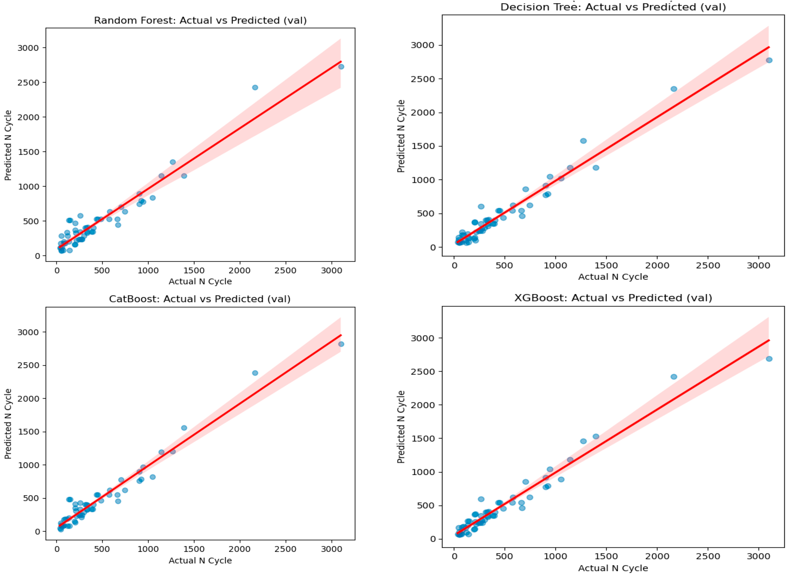
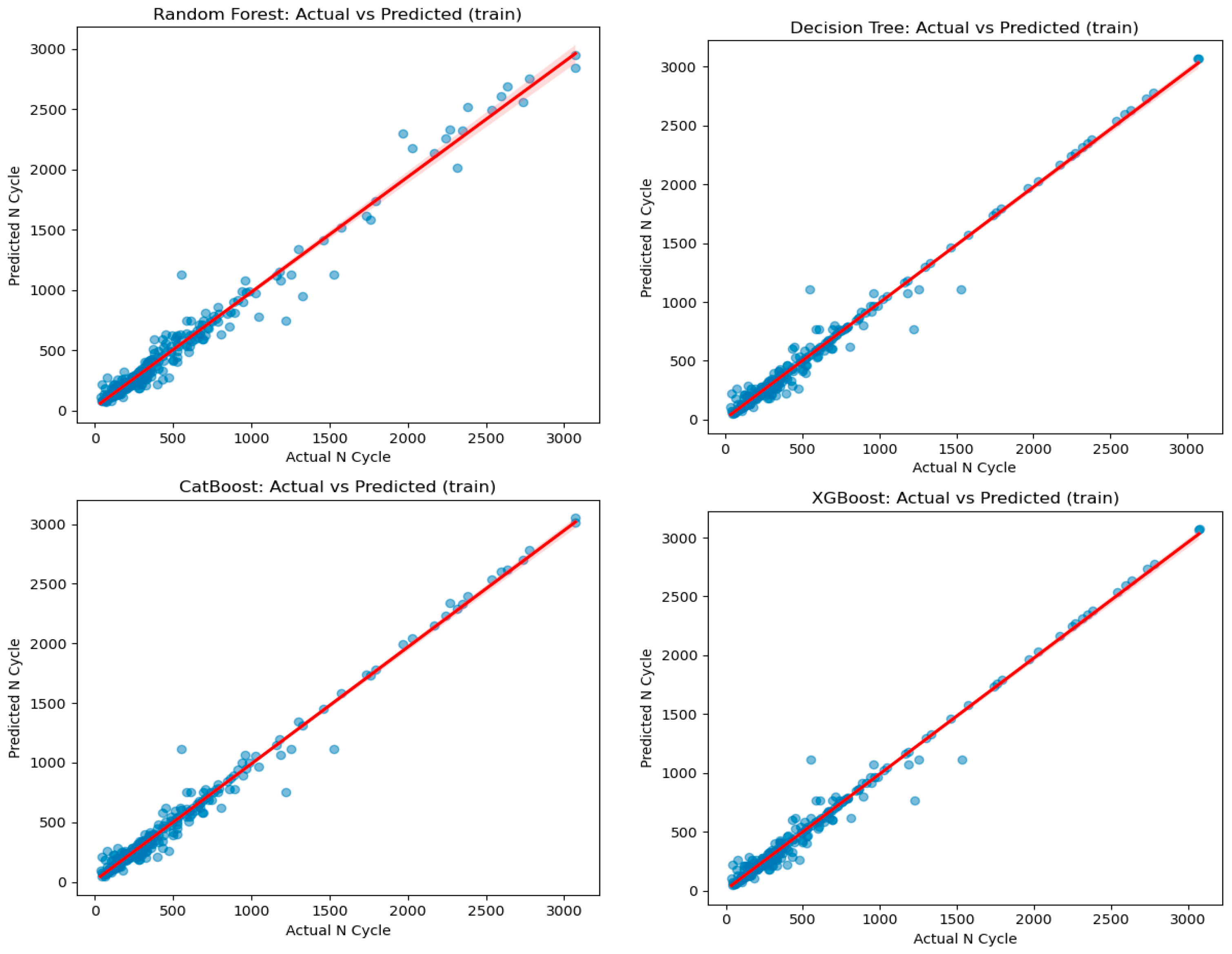
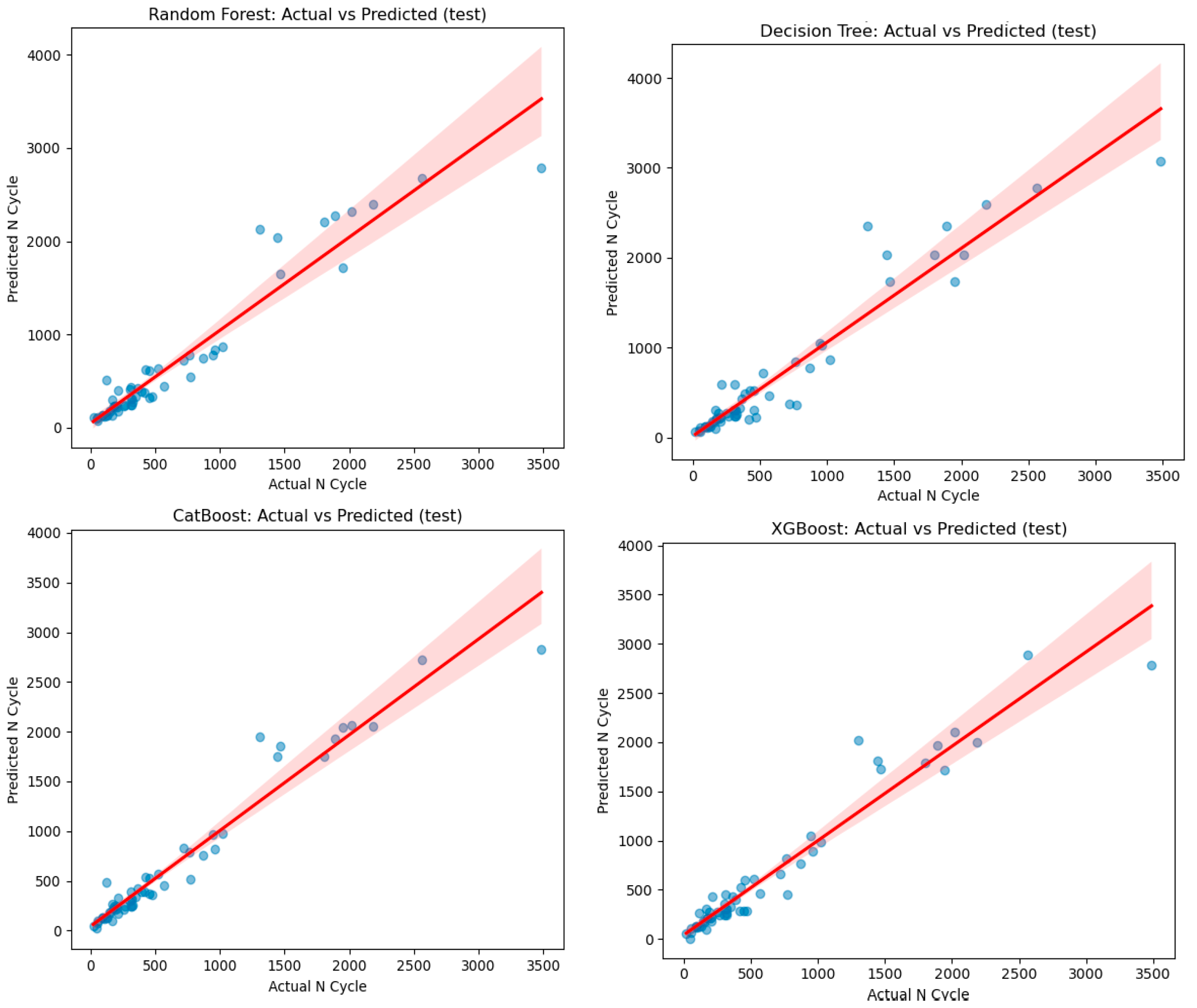
6. Results Analysis and Interpretation

Each model was assessed based on its mean absolute error (MAE), R² score, and mean squared error (MSE). Additionally, a neural network was developed and trained to further explore deep learning’s potential in predicting the N cycle, as shown in

Table 2. Summary of ML results.

	R2 Train	MSE Train	MAE Train	MAPE Train	R2 Test	MSE Test	MAE Test	MAPE Test	R2 Val	MSE Val	MAE Val	MAPE Val
Linear Regression	0.79	71,043.3	162.86	41.6	0.74	137,571	179.6	95.2	0.17	238,488	227	102.6
Decision Tree	0.98	5325.93	34.49	13.93	0.90	52,927.47	140.34	31.18	0.96	12,851.32	81.48	34.31
Random Forest	0.97	8808.89	58.99	20.92	0.91	46,218.97	133.08	36.72	0.93	21,229.60	106.67	60.11
CatBoost	0.98	5676.25	42.42	16.16	0.95	26,838.36	94.67	26.41	0.95	13,412.97	83.05	36.38
XGBoost	0.98	5326.35	34.72	13.99	0.94	32,084.48	109.97	27.97	0.95	13,372.35	83.24	34.29
SVR	−0.11	380,259.08	344.41	92.22	−0.18	617,471.00	453.79	114.22	−0.07	308,336.33	320.95	132.93
ANN	−2297.66	786,764,411.21	23,004.33	10,138.22	−1366.43	714,863,123.33	22,284.46	9517.33	−3439.14	991,063,768.03	23,647.49	16,981.80

. The analysis is focused on the best four models that demonstrated good results (namely CatBoost, XGBoost, Random Forest, and Decision Tree). The other models (SVR, LR, and ANN) will be ignored as they fail to learn patterns because of the following potential reasons:

• Model overfitting (occurs when a model is overly complex in training data or fails when tested).
• The dataset might be too small or noisy.

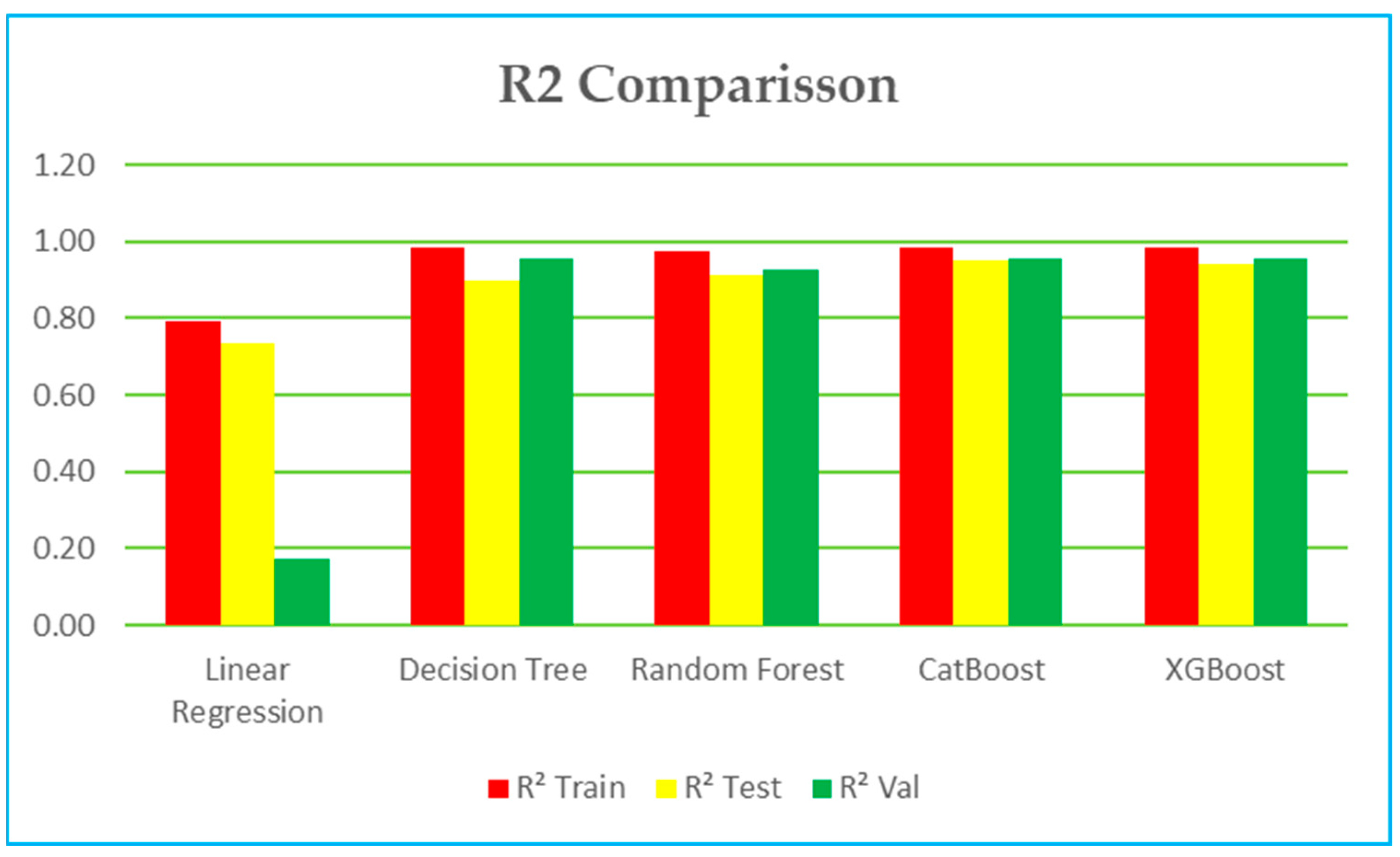
6.1. R² (Coefficient of Determination)—Figure 6

• Training: Both CatBoost, Decision Tree and XGBoost perform similarly with 0.98, followed by Random Forest with 0.97
• Testing: CatBoost performance is slightly better with 0.95 compared to XGBoost with 0.945, Random Forest with 0.91 and Decision Tree with 0.90.
• Validation: Decision Tree with 0.96, both CatBoost and XGBoost with 0.95 and Random Forest with 0.96.
• The other models result in poor modeling outputs.

Figure 6. Model comparison-based R².

Figure 6. Model comparison-based R².

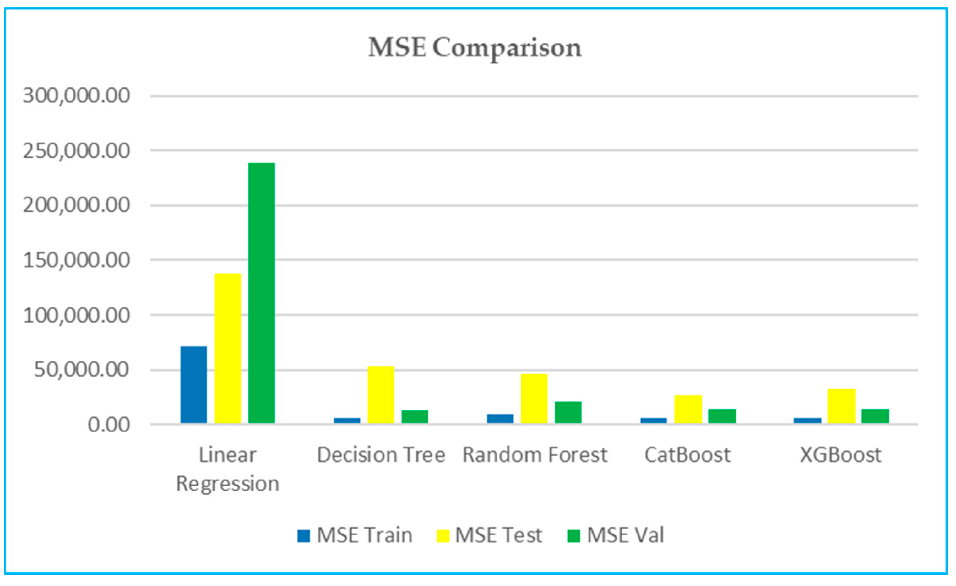
6.2. MSE (Mean Squared Error)—Figure 7

▪

Training: XGBoost and Decision Tree have a lower training MSE (5326, 5325, respectively), indicating that they fit the training data better than CatBoost 5676 and Random Forest with 8808.

▪

Testing and validation: XGBoost and CatBoost perform better in testing, but in validation, Decision Tree and CatBoost are better than XGBoost and Random Forest.

Figure 7. Model comparison-based MSE.

Figure 7. Model comparison-based MSE.

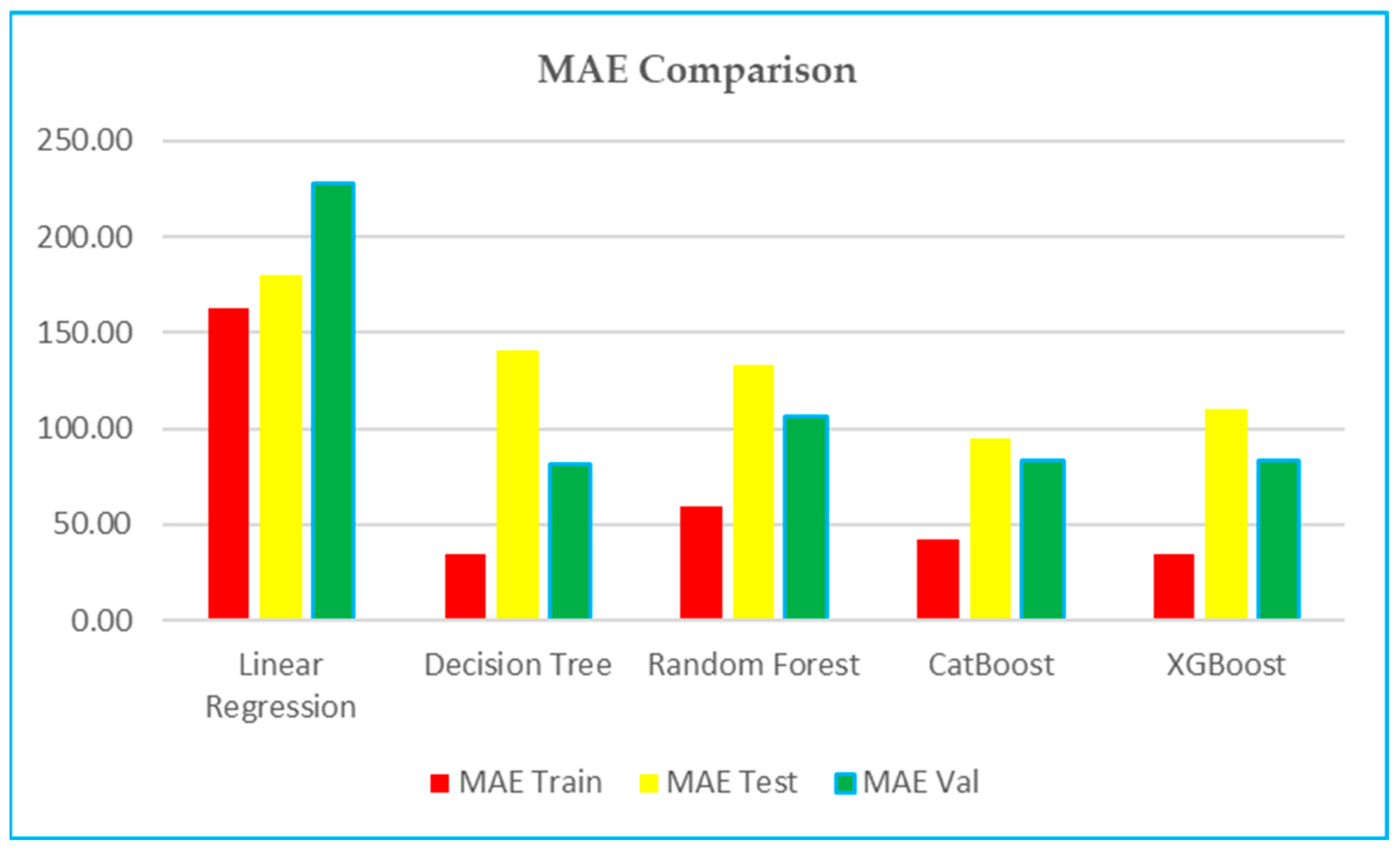
6.3. MAE (Mean Absolute Error)—Figure 8

• Training: Decision Tree and XGBoost have a lower training MAE, at 34.49 and 34.49, respectively, compared to CatBoost at 42.42 and Random Forest at 58.99.
• Testing: CatBoost performs marginally better than XGBoost (94.67–109.97). Random Forest is slightly better than Decision Tree (133.08 vs. 140.34).
• Validation: Random Forest has a lower validation MAE (51.79 vs. 57.30).

Figure 8. Model comparison-based MAE.

Figure 8. Model comparison-based MAE.

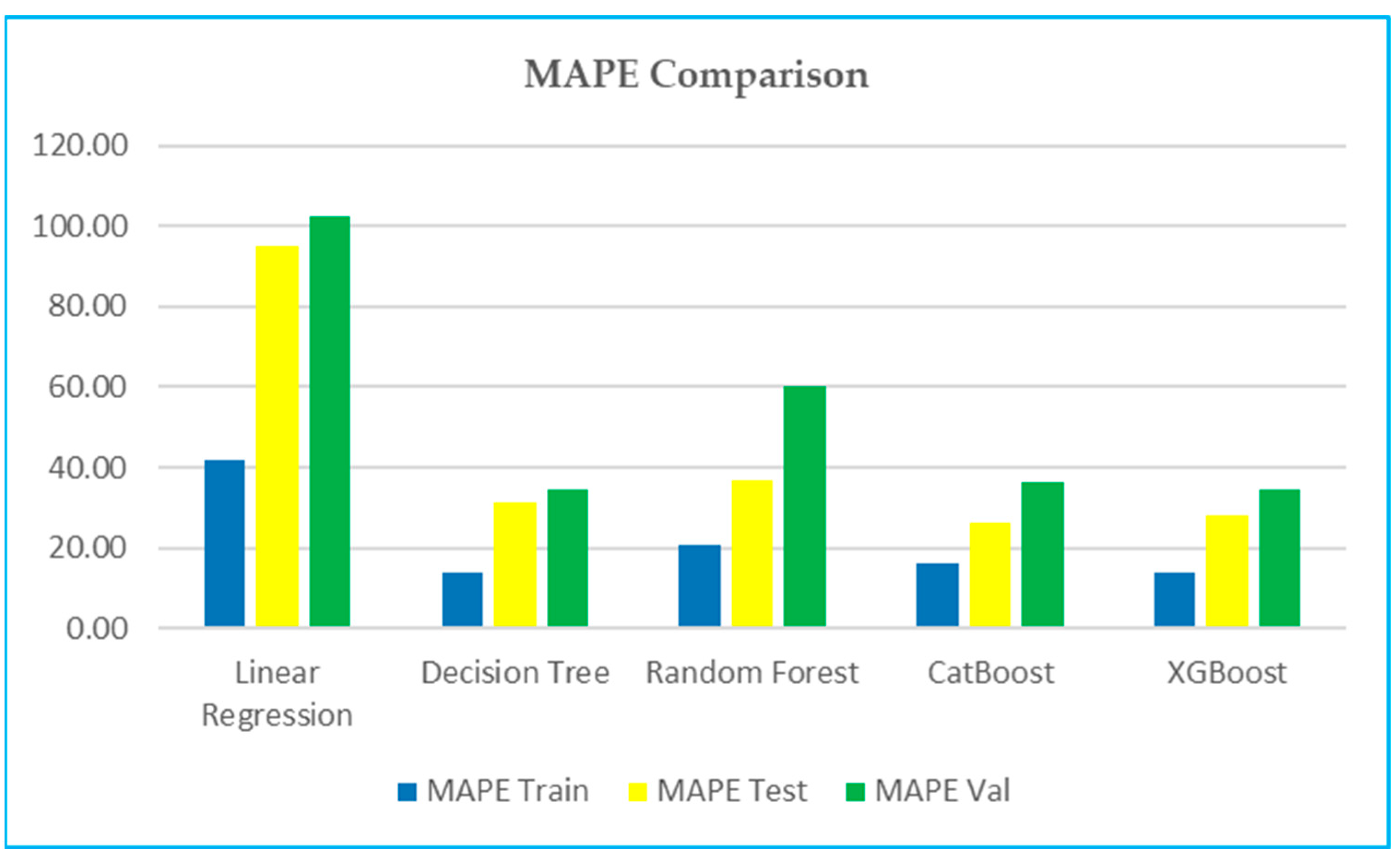
6.4. MAPE (Mean Absolute Percentage Error)—Figure 9

• Training: XGBoost and Decision Tree have a significantly lower training MAPE (13.99 and 13.93, respectively) indicating better percentage error performance during training.
• Testing and validation: CatBoost and XGBoost demonstrate slightly better performance in testing, but in validation sets, XGBoost and Decision Tree demonstrate better performance.

Figure 9. Model comparison-based MAPE.

Figure 9. Model comparison-based MAPE.

6.5. Model Performance Analysis

The results from our machine learning analysis demonstrate that CatBoost and XGBoost are the most suitable models for fatigue life prediction. These models exhibited high predictive accuracy, with R² values exceeding 0.94 on the test set, alongside relatively low error metrics (MSE, MAE, and MAPE), indicating strong generalization capability. Their ability to effectively capture complex, non-linear relationships make them well suited for fatigue life modeling, where interactions between material properties, welding effects, and operational stress conditions significantly influence failure cycles. While Decision Tree and Random Forest models also performed well, they exhibited higher error rates compared to boosting methods, suggesting a need for further optimization through hyperparameter tuning and pruning to prevent overfitting. Linear regression, on the other hand, proved inadequate, as it assumes a linear relationship between input variables and fatigue life, which contradicts the inherently non-linear nature of fatigue damage accumulation in materials subjected to cyclic loading.

Notably, support vector regression (SVR) and artificial neural networks (ANNs) failed to deliver reliable predictions. SVR struggled to identify meaningful support vectors, leading to poor generalization and high prediction errors. The ANN model exhibited severe instability and overfitting, likely due to an improper network architecture, insufficient data, or a lack of regularization, resulting in an extreme negative R² value during validation. These findings emphasize the importance of careful model selection and tuning, particularly when dealing with fatigue life data, where non-linear dependencies and feature interactions are crucial.

In conclusion, gradient boosting methods (CatBoost and XGBoost) offer the best balance between accuracy, stability, and interpretability, making them the preferred choice for fatigue life prediction. On the other hand, while tree-based models like CatBoost and XGBoost demonstrate strong predictive performance, the use of machine learning in engineering applications comes with certain limitations that must be acknowledged. Primary concerns include the interpretability of ML models, their dependency on high-quality training data, the challenge of generalization to unseen conditions, and the need for ethical considerations in safety-critical applications. To address these concerns, a correlation analysis based on SHAP, feature importance analysis, and partial dependence plots was performed to enhance interpretability and is outlined in the following section.

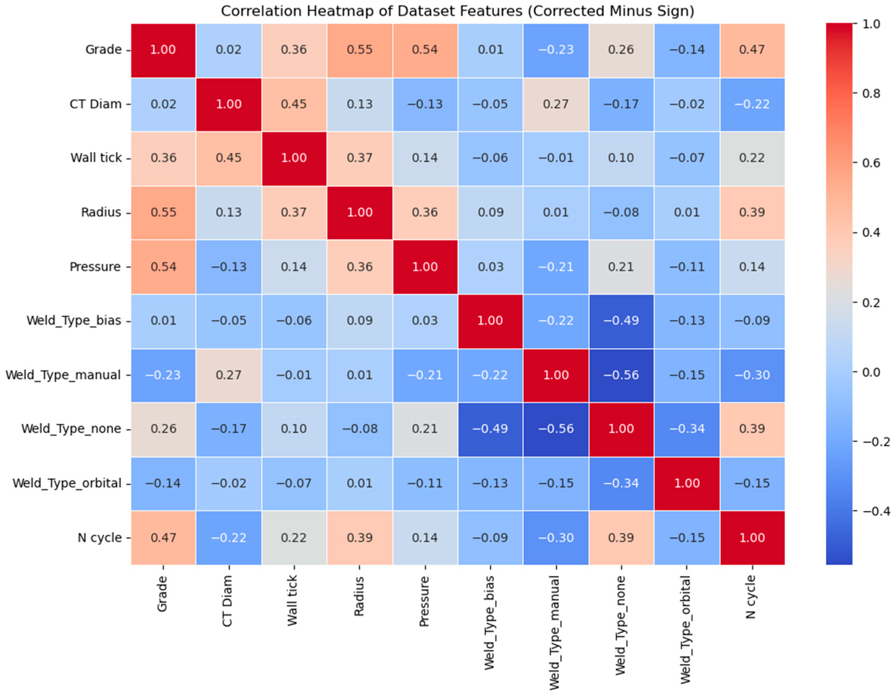
7. Correlation Analysis

7.1. Heatmap Correlation

The correlation heatmap (Figure 10) provides valuable insights into the mechanistic influence of various parameters on the fatigue life of coiled tubing, as measured in N cycles. A detailed examination of the correlation values allows us to identify key factors that either enhance or degrade fatigue resistance in the material.

Among the positively correlated features, wall thickness (+0.26) shows a moderate correlation with fatigue life, suggesting that increasing the wall thickness improves fatigue resistance. Mechanistically, thicker walls mitigate stress concentrations, delaying the initiation and propagation of fatigue cracks. Similarly, the absence of welds (Weld_Type_none, +0.37) significantly enhances fatigue life, as welding often introduces discontinuities, residual stresses, and metallurgical defects that can act as crack initiation sites. Additionally, bending radius (+0.30) exhibits a positive correlation, indicating that a larger bending radius reduces strain-induced damage, thereby extending fatigue life.

Conversely, several features exhibit a negative correlation with fatigue life, indicating detrimental effects. Coiled tubing diameter (−0.29) negatively affects fatigue performance, which can be attributed to the fact that larger diameters undergo greater bending stresses during repeated coiling and uncoiling operations, accelerating crack growth. Similarly, manual welding (−0.39) has the strongest negative correlation, highlighting the adverse effects of inconsistencies in manually welded sections, which introduce defects such as porosity, incomplete fusion, and higher residual stresses that reduce fatigue resistance. Even orbital welding (−0.16), which is generally more consistent than manual methods, exhibits a negative correlation due to the heat-affected zone (HAZ) altering material properties and reducing fatigue resistance. Other parameters demonstrate weaker correlations with fatigue life. Material grade (+0.24) shows a slight positive influence, suggesting that higher-strength materials offer improved resistance to cyclic loading, likely due to their refined microstructure and better fatigue crack resistance. Operating pressure (−0.06), despite being a crucial factor in wellbore operations, exhibits a weak negative correlation, implying that bending loads dominate fatigue damage mechanisms more than internal pressure fluctuations.

Table 3. Summary of mechanistic feature impact on fatigue life of CT.

Mechanistic Summary
Feature	Correlation with N Cycle	Mechanistic Explanation
Wall Thickness	0.26	Thicker walls reduce stress concentration, delaying fatigue failure.
Weld_Type_none	0.37	No welds = No defects, better fatigue resistance.
CT Diameter	−0.29	Larger diameter → Higher bending stress → Lower fatigue life.
Weld_Type_manual	−0.39	Manual welding introduces defects and residual stress, reducing fatigue life.
Weld_Type_orbital	−0.16	Orbital welding still causes some HAZ effects, slightly reducing fatigue life.
Grade	0.24	Higher grades offer better fatigue resistance.
Pressure	−0.06	Weak influence; bending loads dominate over internal pressure.
Radius	0.3	Larger bending radius reduces strain, increasing fatigue life.

presents a summary of the impact of mechanistic features on the fatigue life of CT.

In conclusion, this analysis highlights the influence of welding methods, tubing diameter, and bending radius on fatigue life. Strategies to improve fatigue resistance should emphasize minimizing welding defects, optimizing tubing geometry, and increasing bending radius to reduce cyclic strain.

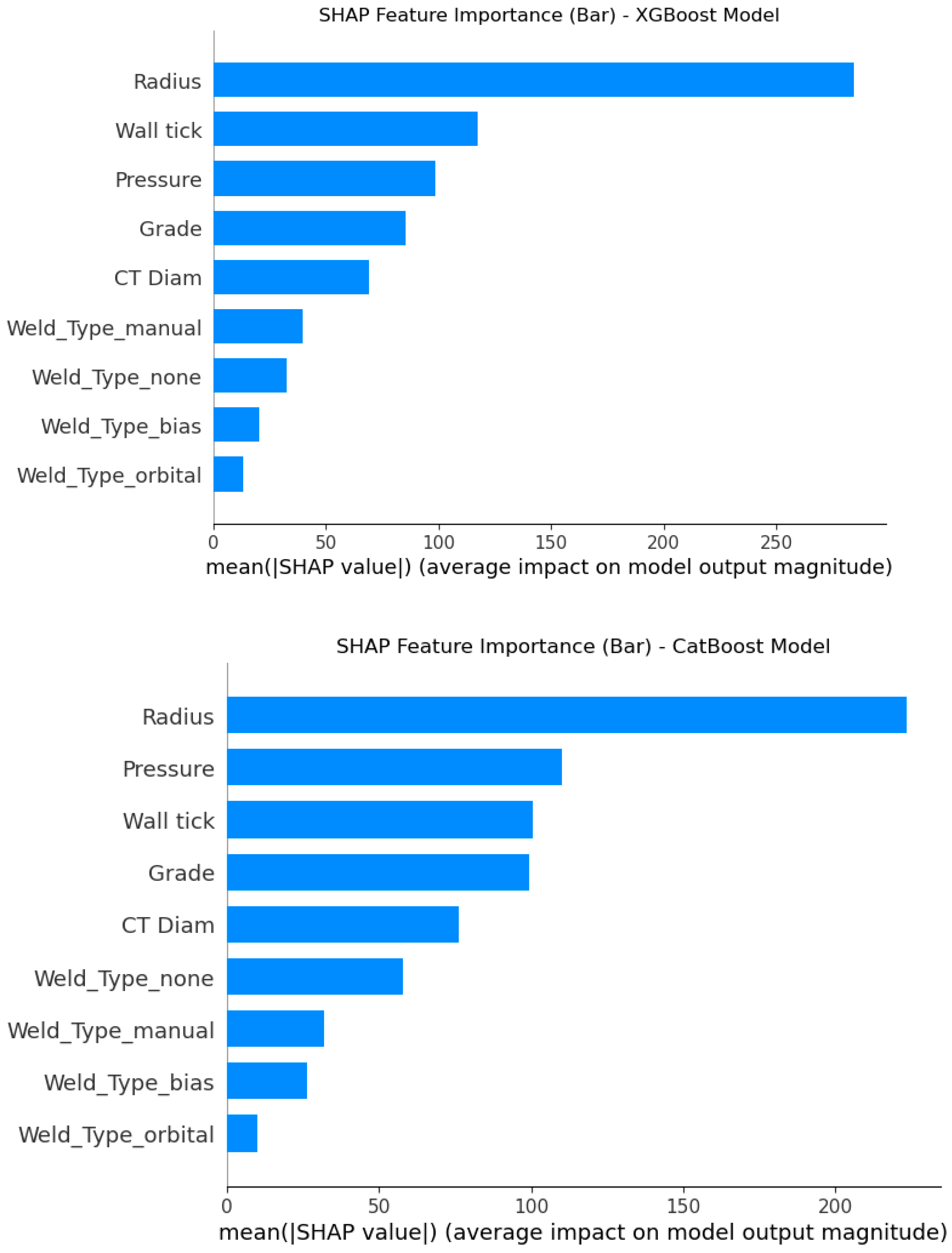
7.2. SHAP Feature Importance Analysis

SHAP feature importance analysis revealed that wall thickness, weld type, and pressure were the most dominant factors affecting fatigue life predictions (Figure 11). These findings align with material science principles, where thinner sections experience higher stress concentrations, which accelerate fatigue crack initiation. Similarly, welds introduce residual stresses and discontinuities that significantly reduce fatigue resistance. The high feature importance assigned to pressure reflects its role in influencing hoop stress, which contributes to fatigue damage over multiple cycles. These results confirm that ML models are not only data-driven but also align with established fatigue life theories.

7.3. Influence of Dominant Features on Fatigue Behavior

7.3.1. Radius of Curvature: The Most Significant Factor

The radius of curvature emerged as the strongest predictor of fatigue life in both models. A smaller radius results in higher localized bending stress, accelerating fatigue crack initiation and propagation. This aligns with the elastic–plastic fatigue theory, where stress concentration increases exponentially as the radius decreases, leading to early failure.

The ML models identified radius as the most critical feature, confirming established fatigue mechanisms in coiled tubing operations.

7.3.2. Material Grade: Direct Influence on Fatigue Resistance

Material grade was ranked as the second most important factor, affecting fatigue resistance through mechanical properties such as yield strength, hardness, and micro structural stability. This is explained by the fact that the higher-grade materials exhibit enhanced endurance limits, resisting cyclic strain accumulation and delaying fatigue crack initiation. The models reinforced that material strength correlates with fatigue life, supporting empirical observations from strain–life and stress–life fatigue models.

7.3.3. Wall Thickness: Stress Distribution Impact

Moderate influence was observed for wall thickness, indicating that while thicker tubing can better distribute stress, other factors (e.g., bending radius) play a more dominant role. Thicker walls reduce stress intensity factors (SIFs), which slow crack propagation. However, when tubing undergoes repeated bending cycles, the overall strain distribution may still be dictated by geometric constraints rather than just thickness. ML models recognize wall thickness as a secondary factor, aligning with structural fatigue theories.

7.3.4. Internal Pressure: Limited Direct Effect on Fatigue Life

While internal pressure contributes to hoop stress, its impact on fatigue life was lower than anticipated. This is because the fatigue damage in coiled tubing is primarily driven by cyclic bending stress, with hoop stress playing a secondary role, unless the tubing operates near the plastic deformation limits. The models assigned less importance to pressure, confirming that mechanical strain dominates fatigue behavior over internal loading effects.

7.3.5. Weld Type

Welding and its type may influence stress concentration and crack initiation. The weld type (manual, orbital, or bias) showed moderate to low importance, indicating that while welding affects fatigue behavior, its impact depends on specific weld geometry and residual stresses. It is known that welding discontinuities and heat-affected zones introduce localized stress concentrations, making them potential fatigue initiation points. However, if the welds are well executed and post-treated, their impact may be minimized. ML models acknowledge welds as a factor, but not a primary driver, of fatigue, suggesting that well-controlled welding processes can mitigate their influence.

7.3.6. Engineering Implications of ML-Driven Feature Importance

Analysis

The consistency between machine learning feature importance results and well-established material fatigue principles confirms the validity of the predictive models. These findings provide several engineering insights that can be leveraged for fatigue life optimization:

• Reducing the bending radius significantly shortens fatigue life → Designing tubing with larger radii, where feasible, can increase operational lifespan.
• Higher-grade materials exhibit greater fatigue resistance → Material selection should prioritize grades with superior fatigue endurance properties.
• Wall thickness improves fatigue resistance but is not the primary driver → Optimizing tubing thickness alone will not compensate for poor radius selection.
• Internal pressure effects on fatigue life are secondary → Operators should focus more on cyclic bending stress management instead of just pressure control.
• Welding effects can be minimized through quality control → Proper welding techniques and post-weld treatments (e.g., stress relief and shot peening) can help reduce fatigue-related failures.

7.4. Conclusions

The results from XGBoost and CatBoost feature importance analysis align closely with known fatigue life prediction models, reinforcing the credibility of data-driven approaches in fatigue modeling. By integrating ML models with material science principles, engineers can make informed decisions to optimize coiled tubing design, reduce failure rates, and extend service life.

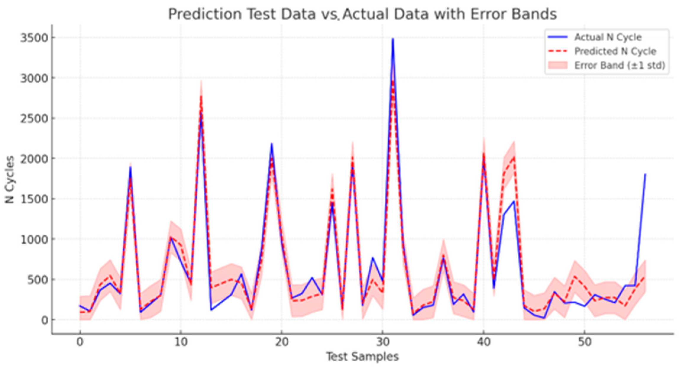
8. Prediction Analysis

ML Modeling Analysis

The CatBoost and XGBoost models demonstrated strong performance when predicting the cycle for the test dataset, as evidenced by the actual versus predicted plots (Figure 12). The majority of the points are closely clustered around the ideal fit line, which represents perfect predictions.

This indicates that the model accurately treated the underlying patterns in the data and made reasonable predictions across a wide range of values, particularly in the interval between 200 and 800, where the predictions of the models closely matched the actual values (Figure 12, Figure 13, Figure 14 and Figure 15). However, outside this interval, it is remarkable how much less ability there is to predict, as shown by the models that can be improved by conducting a more accurate fatigue test and increasing the amount of data that can effectively provide the machine learning system with the means to train the models, thereby enhancing their predictive ability and reducing deviations from the ideal fit line.

In the above figures the blue dots represent actual vs predicted values, where each dot corresponds to a test sample. The red line is the best-fit regression line, indicating perfect predictions if all points lie on it. The shaded region around the line represents confidence intervals or model uncertainty. If the blue dots are close to the red line, the model performs well; deviations indicate prediction errors. All models seem accurate but show some errors at higher N Cycle values, possibly due to overfitting or difficulty predicting extreme cases.

To further enhance the model’s accuracy, particularly at these extremes, it would be beneficial to investigate the data points with the largest errors and assess whether they are outliers or represent unique patterns. Additionally, further hyperparameter tuning and feature engineering—including creating new interaction terms or applying transformations to the existing features—might help the model generalize better across the full range of N cycle values.

Overall, the XGBoost and CatBoost regressor models show good predictivity power despite the quantity and the complexity of the dataset, offering an effective tool for fatigue life prediction tasks.

9. General Conclusions

With the revolution in AI and machine learning methods, predicting material fatigue behavior in terms of fatigue life has become easier to track and more accurate. This study takes a step toward tackling this phenomenon by gathering a large amount of fatigue testing data, which represents the first condition for effective machine learning.

The techniques applied have demonstrated strong performance in predicting CT fatigue life, forming the foundation for a proper modeling and tracking process to be implemented in field applications.

This study demonstrated the effectiveness of using machine learning to handle complicated problems that are difficult to model analytically. Due to its ability to manage a large, complex, and non-linear dataset (analyzing, training, and testing), machine learning aids in effectively studying material fatigue behavior, enabling us to apply this beneficial and powerful tool to successfully study the fatigue of coiled tubing in comparison to traditional methods.

This study explored the estimation of coiled tubing fatigue life by analyzing the performance of different machine learning models. The outcomes revealed that gradient boosting regression algorithms, namely CatBoost and XGBoost, consistently surpassed other models in terms of accuracy, as indicated by the R², MAE, and MSE metrics. These results emphasize the ability of advanced machine learning approaches to enhance fatigue life predictions, contributing to the improved dependability and efficiency of coiled tubing operations in well interventions. Proper modeling enhances the prediction of CT fatigue evolution. This modeling step forms the basis of a monitoring and tracking process that can help to prevent CT failures in advance and optimize CT’s service safely and successfully.

Overall, this research highlights the importance of using and choosing the most optimal machine learning models for predicting coiled tubing fatigue, such as Gradient Boosting models (CatBoost and XG Boost), making them valuable tools for engineers in predictive maintenance and structural reliability.

References

1. Neog, D.; Sarmah, A.; Baruah, M.I.S. Computational analysis of coiled tubing concerns during oil well intervention in the upper Assam basin, India. Sci. Rep. 2023, 13, 1795. [Google Scholar] [CrossRef] [PubMed]
2. Li, Y.; Gao, X.-L.; Ni, L.; Hu, Q.; Xin, Y. Fatigue of coiled tubing and its influencing factors: A comparative study. In Proceedings of the ASME International Mechanical Engineering Congress and Exposition, Phoenix, AZ, USA, 11–17 November 2016. [Google Scholar]
3. Shaohu, L.; Feng, G.; Xianjin, W.; Hui, X.; Zhen, W.; Ting, Y. Theoretical and experimental research of bearing capacity and fatigue life for coiled tubing under internal pressure. Eng. Fail. Anal. 2019, 104, 1133–1142. [Google Scholar] [CrossRef]
4. Bridge, C. Combining elastic and plastic fatigue damage in steel pipelines, risers, and coiled tubing. SPE Drill. Complet. 2012, 27, 493–500. [Google Scholar] [CrossRef]
5. Zhao, G.; Zhong, J.; Feng, C.; Liang, Z. Simulation of ultra-low cycle fatigue cracking of coiled tubing steel based on cohesive zone model. Eng. Fract. Mech. 2020, 235, 107201. [Google Scholar] [CrossRef]
6. Chen, J.; Liu, Y. Fatigue modeling using neural networks: A comprehensive review. Fatigue Fract. Eng. Mater. Struct. 2022, 45, 945–979. [Google Scholar] [CrossRef]
7. Tipton, S.M. Multiaxial plasticity and fatigue life prediction in coiled tubing. In Advances in Fatigue Lifetime Predictive Techniques: 3rd Volume; ASTM International: West Conshohocken, PA, USA, 1996. [Google Scholar]
8. Newman, K.R. Development of a new CT life tracking process. In Proceedings of the SPE/ICoTA Well Intervention Conference and Exhibition, The Woodlands, TX, USA, 26–27 March 2013; p. SPE 163884. [Google Scholar]
9. Milella, P.P. Strain-Based Fatigue Analysis—Low Cycle Fatigue. In Fatigue and Corrosion in Metals; Springer: Berlin/Heidelberg, Germany, 2024; pp. 355–411. [Google Scholar]
10. Newman, K.; Kelleher, P. CT Fatigue Modeling Update. In Proceedings of the SPE/ICoTA Well Intervention Conference and Exhibition, Houston, TX, USA, 22–23 March 2016; p. SPE 179049. [Google Scholar]
11. Wu, J. Coiled tubing working life prediction. In Proceedings of the SPE Oklahoma City Oil and Gas Symposium/Production and Operations Symposium, Oklahoma City, OK, USA, 2–4 April 1995. [Google Scholar]
12. Tipton, S.M. The Achilles Fatigue Model; CTES LP User Technical Note; CTES: Conroe, TX, USA, 1999. [Google Scholar]
13. Avakov, V.A.; Martin, J. Large Coiled Tubing Fatigue Life. In Proceedings of the SPE/ICoTA Well Intervention Conference and Exhibition, San Antonio, TX, USA, 5–8 October 1997; p. SPE 38407. [Google Scholar]
14. Tian, X.; Zhang, H.; Duan, Q.; Ji, Y. Establishment and application of fatigue life prediction models for coiled tubing. In Proceedings of the Pressure Vessels and Piping Conference, Boston, MA, USA, 19–23 July 2015. [Google Scholar]
15. Liu, B.; Li, T.; Xu, L.; Han, B.; Zhuang, H.; Li, S. Effect of surface defects and internal pressure on fatigue life of coiled tubing. In Proceedings of the 9th China-Russia Symposium “Coal in the 21st Century: Mining, Intelligent Equipment and Environment Protection” (COAL 2018), Qingdao, China, 18–21 October 2018; pp. 185–189. [Google Scholar]
16. Zhong, J.; Guanghui, Z.; Litong, W.; Yi, H.; Sihai, H. Experimental and Numerical Study on LCF Crack Propagation of Coiled Tubing Steel. Mechanics 2022, 28, 351–357. [Google Scholar] [CrossRef]
17. Bunge, J.M.; Coloschi, M.; Cravero, S.; Valdez, M.; Reichert, B.; Grimaldo, C. Coiled Tubing Premature Failure–The Effects of Pressure and Strain. In Proceedings of the SPE/ICoTA Well Intervention Conference and Exhibition, The Woodlands, TX, USA, 22–23 March 2022; p. SPE 208996. [Google Scholar]
18. Padron, T.; Aitken, B. CT100+ Bias Weld Fatigue Life Estimations-Are Adjustments Required? In Proceedings of the SPE/ICoTA Well Intervention Conference and Exhibition, Houston, TX, USA, 22–23 March 2016; p. SPE 179045. [Google Scholar]
19. Ishak, J.; Santos, M.A.; Tipton, S.M. Numerical and Experimental Analysis of Cyclic Strains in Coiled Tubing Surface Defects for Fatigue Life Assessment. In Proceedings of the SPE/ICoTA Well Intervention Conference and Exhibition, Houston, TX, USA, 21–22 March 2017; p. SPE 184761. [Google Scholar]
20. Sherman, S.; Majko, S.M.; Otto, J. High Strength Coiled Tubing-How is Fatigue Life Affected by Slip Damage? In Proceedings of the SPE/ICoTA Well Intervention Conference and Exhibition, The Woodlands, TX, USA, 24 March 2020; p. SPE 199859. [Google Scholar]
21. Faszold, J.; Rosine, R.; Spoering, R. Full-Scale Fatigue Testing With 130K Yield Tubing. In Proceedings of the SPE/ICoTA Well Intervention Conference and Exhibition, The Woodlands, TX, USA, 27–28 March 2012; p. SPE 153945. [Google Scholar]
22. Tipton, S.M.; Smalley, E.; VanArnam, D. Influence of a straightener on coiled tubing fatigue. In Proceedings of the SPE/ICoTA Well Intervention Conference and Exhibition, The Woodlands, TX, USA, 27–28 March 2012. [Google Scholar]
23. Headrick, D.; Rosine, R. Full-scale coiled tubing fatigue tests with tubing pressures to 15,000 psi. In Proceedings of the SPE/ICoTA Well Intervention Conference and Exhibition, Houston, TX, USA, 25–26 May 1999; p. SPE 54482. [Google Scholar]
24. Reichert, B.; Nguyen, T.; Rolovic, R.; Newman, K. Advancements in Fatigue Testing and Analysis. In Proceedings of the SPE/ICoTA Well Intervention Conference and Exhibition, Houston, TX, USA, 22–23 March 2016; p. SPE 179064. [Google Scholar]
25. Association, D.E. Underbalanced Drilling and Completion Manual, DEA; Maurer Engineering Inc.: Austin, TX, USA, 1996; p. 101. [Google Scholar]
26. Falcone, R.; Lima, C.; Martinelli, E. Soft computing techniques in structural and earthquake engineering: A literature review. Eng. Struct. 2020, 207, 110269. [Google Scholar] [CrossRef]
27. Yang, D.; Jin, A.; Li, Y. A Novel Physics-Guided Neural Network for Predicting Fatigue Life of Materials. Appl. Sci. 2024, 14, 2502. [Google Scholar] [CrossRef]
28. Peng, S.; Xiao, J.-Q.; Tian, Y.; Zhang, Y.; Feng, J.; Hu, Z.-J. Coiled tubing working life prediction based on BP algorithm of artificial neural network. In Proceedings of the IADC/SPE Asia Pacific Drilling Technology Conference and Exhibition? Tianjin, China, 9–11 July 2012. [Google Scholar]
29. Newman, K.; Brown, P. Development of a standard coiled-tubing fatigue test. In Proceedings of the SPE Annual Technical Conference and Exhibition? Houston, TX, USA, 3–6 October 1993; p. SPE 26539. [Google Scholar]
30. Zhang, L.-G.; Yue, Q.-B.; Luo, M. The prediction of the low cycle fatigue life about the coiled tubing with ovality and wall thickness. J. Fail. Anal. Prev. 2017, 17, 1288–1296. [Google Scholar] [CrossRef]
31. Rispler, K.; McNichol, J.; Matiasz, K.; Rheinlander, M. Using an artificial neural network to develop a wall-loss model for coiled tubing fracturing operations. In Proceedings of the SPE/ICoTA Well Intervention Conference and Exhibition, Houston, TX, USA, 7–8 March 2001; p. SPE 68420. [Google Scholar]
32. Sisak, W.; Crawford, D. The fatigue life of coiled tubing. In Proceedings of the SPE/IADC Drilling Conference and Exhibition, Dallas, TX, USA, 15–18 February 1994; p. SPE 27437. [Google Scholar]
33. Elliott, K.; Graham-Wright, T.; Williams, C.; Hampson, R.; Portillo, B.; Cuaron, A. Development and Compatibility Testing of Coiled Tubing with 140-ksi Specified Minimum Yield Strength. In Proceedings of the SPE/ICoTA Well Intervention Conference and Exhibition, Houston, TX, USA, 21–22 March 2017; p. SPE 184806. [Google Scholar]
34. Chitwood, G.; Lewis, P.; Fowler, S.; Zernick, W. High-Strength Coiled Tubing Expands Service Capabilities. In Proceedings of the Offshore Technology Conference, Houston, TX, USA, 24 May 1992; p. OTC 7032-MS. [Google Scholar]
35. VanArnam, W.D.; Hargis, C. New Higher-Strength Coiled Tubing Developed To Extend Coiled Tubing Operating Envelopes. In Proceedings of the SPE/ICoTA Well Intervention Conference and Exhibition, The Woodlands, TX, USA, 5–6 April 2011; p. SPE 143152. [Google Scholar]
36. Brown, P.A.; Arnam, D.V. Coiled Tubing Weld Cycle Life. 1995. Available online: https://www.athenaeng.com/publications/1995_10_DEA_97_CT_Weld_Cycle_Life_Report.pdf (accessed on 1 March 2025).
37. Shaohu, L.; Hao, Z.; Hui, X.; Quanquan, G. A new theoretical model of low cycle fatigue life for coiled tubing under coupling load. Eng. Fail. Anal. 2021, 124, 105365. [Google Scholar] [CrossRef]
38. Padron, T.; Datahan, G. Effect of external mechanical damage on the fatigue life of coiled tubing exposed to sour environments: Criteria for CT100 grade. In Proceedings of the SPE/ICoTA Well Intervention Conference and Exhibition, The Woodlands, TX, USA, 31 March–1 April 2009. [Google Scholar]
39. Valdez, M.; Morales, C.; Rolovic, R.; Reichert, B. The development of high-strength coiled tubing with improved fatigue performance and H2S resistance. In Proceedings of the SPE/ICoTA Well Intervention Conference and Exhibition, The Woodlands, TX, USA, 24–25 March 2015; p. SPE 173639. [Google Scholar]
Figure 1. Machine learning in material fatigue.
Applsci 15 02899 g001
Figure 2. Conventional vs. proposed ML methodology for CT fatigue life estimation.
Applsci 15 02899 g002
Figure 3. Full-scale fatigue testing equipment [23].
Applsci 15 02899 g003
Figure 4. Lab-scale fatigue testing machine [2,39].
Applsci 15 02899 g004
Figure 5. Flowchart process for predicting fatigue life (N cycle).
Applsci 15 02899 g005
Figure 10. Correlation analysis between features and N cycle.
Applsci 15 02899 g010
Figure 11. Feature importance impact on fatigue life of CT for best ML models.
Applsci 15 02899 g011
Figure 12. Prediction plot for the best model with test data vs. actual data.
Applsci 15 02899 g012
Figure 13. Prediction plot for the best models with Val data vs. actual data (Random Forest, Decision Tree, XGBoost and CatBoost).
Applsci 15 02899 g013
Figure 14. Prediction plot for the best models with train data vs. actual data (Random Forest, Decision Tree, XGBoost and CatBoost).
Applsci 15 02899 g014
Figure 15. Prediction plot for the best models with test data vs. actual data (Random Forest, Decision Tree, XGBoost and CatBoost).
Applsci 15 02899 g015