Modeling and Estimating LIDAR Intensity for Automotive Surfaces Using Gaussian Process Regression: An Experimental and Case Study Approach

Abstract

LIDAR technology is widely used in autonomous driving and environmental sensing, but its accuracy is significantly affected by variations in vehicle surface reflectivity. This study models and predicts the impact of different LIDAR sensor specifications and vehicle surface paints on laser intensity measurements. Laser intensity data from the experiments of Shung et al. were analyzed alongside vehicle color, angle, and distance. Multiple machine learning models were tested, with Gaussian Process Regression (GPR) performing best (RMSE = 0.87451, R² = 0.99924). To enhance the model’s physical interpretability, laser intensity values were correlated with LIDAR optical power equations, and curve fitting was applied to refine the relationship. The model was validated using the input parameters from Shung et al.’s experiments, comparing predicted intensity values with reference measurements. The results show that the model achieves an overall accuracy of 99% and is successful in laser intensity prediction. To assess real-world performance, the model was tested on the CUPAC dataset, which includes various traffic and weather conditions. Spatial filtering was applied to isolate laser intensities reflected only from the vehicle surface. The highest accuracy, 98.891%, was achieved for the SW-Gloss (White) surface, while the lowest accuracy, 98.195%, was recorded for the SB-Matte (Black) surface. The results confirm that the model effectively predicts laser intensity across different surface reflectivity conditions and remains robust across different channels LIDAR systems.

1. Introduction

LIDAR (Light Detection and Ranging) technology utilizes light waves to detect signals reflected from objects, enabling the creation of a detailed environmental map. Enhanced by high-speed processors and advanced computational models, LIDAR systems can simultaneously process large volumes of data points [1]. This technology significantly improves the perception and object recognition capabilities of autonomous driving systems, allowing vehicles to make informed decisions and execute appropriate maneuvers based on real-time environmental data. The performance evaluation of LIDAR systems is conducted through signal processing analyses applied to point cloud datasets. These analyses focus on critical performance parameters, including laser intensity and the number of point clouds (NPC), which are essential for assessing detection accuracy and environmental mapping quality [2].

The performance of LIDAR systems is influenced by various environmental factors, including heavy traffic, fluctuating road conditions, headlight brightness, the color contrast of road signs, and the color variations in surrounding objects. In particular, adverse weather conditions such as rain, fog, dust, and sunlight can lead to the absorption or scattering of LIDAR-emitted light waves through Mie scattering, thereby reducing detection accuracy [3].

LIDAR technology is widely used in autonomous driving and environmental sensing applications due to its high spatial resolution and accuracy. However, it is significantly affected by environmental factors such as surface reflectivity, lighting conditions, and adverse weather. In recent years, advancements in sensing technologies have brought thermal imaging integration into focus, particularly to enhance object recognition in low-visibility conditions. Thermal parameters can provide complementary data to LIDAR intensity measurements, improving object classification and detection in scenarios where objects are camouflaged or where materials have similar reflectivity but different thermal characteristics. This integration can enhance the detection of objects that might otherwise be overlooked or misclassified based on LIDAR intensity alone [4].

In addition, the color and reflectivity properties of vehicles are critical factors influencing the accuracy of LIDAR detection systems. Specifically, black and dark-colored objects, due to their low reflectivity, reduce the detection range and increase the likelihood of data loss. Conversely, highly reflective surfaces can cause the excessive backscattering of emitted light, leading to misleading measurements. For instance, a study has identified three major challenges associated with reflective surfaces in the LIDAR sensing process: (i) When the incident angle is large, a significant portion of the reflected energy fails to reach the sensor, resulting in incomplete measurements. (ii) The secondary reflection of laser beams onto another surface can cause depth overestimation. (iii) Highly reflective surfaces generate a broad intensity spectrum, leading to wave patterns that introduce systematic errors in LIDAR measurements [5].

According to the Euro NCAP test standard, the current LIDAR performance for Advanced Driver Assistance System (ADAS) applications is evaluated using a plain white matte surface with a calibrated reflectance of 90% [6]. However, this test protocol does not account for surfaces with different colors or reflectivity properties, which constitute a significant portion of vehicles on the road. As a result, test setups that do not incorporate real automotive paint types and representative surfaces fail to accurately model the real-world performance of LIDAR systems. Conducting such analyses using existing methods typically requires repetitive experiments, time-consuming data collection processes, and manual evaluations. These limitations hinder the efficiency of analysis processes, restricting both the generalizability and comparability of results across different LIDAR models. Additionally, they constrain a comprehensive evaluation of the impact of various vehicle paint types on LIDAR performance [7]. Variations in the ability of different paint types to reflect, absorb, or scatter laser light introduce significant discrepancies in LIDAR intensity data. When combined with the inherent technical differences between LIDAR models, these variations further complicate the accurate assessment of vehicle paint effects on LIDAR detection performance. Moreover, the variability of LIDAR intensity data due to atmospheric conditions presents an additional challenge, making it difficult to achieve consistent results across different LIDAR models and paint properties. Addressing these complex interactions requires a more systematic and generalizable approach to evaluating the relationship between LIDAR sensors and vehicle surface characteristics [4].

In this context, theoretical analyses and computer-aided modeling techniques play a crucial role in addressing the technical differences between LIDAR sensors and standardizing sensor data [8]. In particular, modeling the relationship between LIDAR intensity values and optical power enables the establishment of a comparable and generalizable framework applicable to both different LIDAR systems and vehicle surface paints. For instance, correlating laser intensity with surface reflectivity and paint color properties facilitates the prediction of how low-reflectivity surfaces, such as dark or matte paints, impact LIDAR detection performance. In this process, methods such as curve fitting techniques, statistical approaches, and machine learning-based algorithms serve as powerful tools for correcting systematic errors in LIDAR intensity data and analyzing the relationships between vehicle surface characteristics and LIDAR performance. These techniques not only contribute to the standardization of variations among different LIDAR sensors but also provide a critical foundation for optimizing the impact of various vehicle paints on LIDAR systems, ultimately enhancing the reliability of environmental perception [9].

Previous studies on factors influencing LIDAR performance have investigated the effects of surface color and reflectivity properties on laser intensity using experimental approaches. Bolkas and Martinez [10] analyzed how surfaces painted in different colors and gloss levels impact LIDAR point cloud noise and scanning geometry. Sequeira et al. [11] examined the influence of vehicle colors on LIDAR detection performance, considering variations in distance and angle. Kim et al. [12] developed pigments designed to enhance near-infrared (NIR) reflectivity, improving the detectability of dark-colored surfaces by LIDAR systems. Additionally, Sabiha et al. [4] experimentally investigated the effects of different automotive paints on LIDAR point cloud density, demonstrating that variations in paint colors and pigment compositions significantly influence LIDAR detection performance. Shung et al. [6] tested the impact of various automotive surface colors on LIDAR systems, analyzing how specific paint types alter laser backscattering properties. Blazek et al. [13] studied the optical properties of different pigments, revealing that a surface’s reflectivity characteristics in the NIR spectrum play a critical role in object detection processes.

Jekal et al. [14] developed next-generation materials with high near-infrared (NIR) reflectivity to enhance LIDAR detectability. In their study, they designed a specialized material called hollow black TiO₂ (HL/BT) to mitigate the low-reflectivity issue of black surfaces, formulating a surface coating that enhances LIDAR signal backscattering. Similarly, Otgonbayar et al. [15] developed novel pigments with high NIR reflectivity to improve the detectability of dark-colored materials by LIDAR and analyzed how their surface properties influence reflectivity performance.

However, the majority of existing studies are experimental in nature, investigating the effects of specific colors and surface coatings on laser intensity solely through direct measurements. Currently, no study in the literature predicts how LIDAR intensity values vary across surfaces with different reflectivity coefficients using modeling and prediction methods. This study fills this gap by developing a statistical and machine learning-based model for laser intensity prediction, integrating the technical specifications of various LIDAR models and the optical properties of vehicle surfaces. The proposed modeling approach extends beyond traditional experimental analyses by providing a generalizable framework for modeling and predicting the impact of surface reflectivity variations on LIDAR laser intensity.

This study aims to model the effects of the technical characteristics of different LIDAR models and vehicle surface paints on laser intensity measurements and to predict the relationships between these effects. The primary objective is to analyze how technical differences among LIDAR sensors—particularly transmitter power variations depending on the number of channels—impact laser intensity performance. In this context, laser intensity data obtained from the experiments conducted by Shung et al., along with variables such as vehicle color, angle, and distance, were utilized in the training and testing processes of various machine learning algorithms. Statistical analyses were conducted on Gaussian Process Regression (GPR), Polynomial Regression, Support Vector Machine (SVM), Decision Tree, Random Forest, and Gradient Boosting algorithms, and their performance in predicting laser intensity values was compared. To enhance the accuracy of the selected model, hyperparameter optimization was conducted using the Bayesian optimization algorithm.

The evaluation of this study was conducted using a Coventry University Public road dataset for Automated Cars (CUPAC) dataset recorded by Coventry University in Coventry, UK, in 2020 [16]. This dataset was utilized to assess the impact of different vehicle surface paints on laser intensity measurements under real-world conditions. In this study, LIDAR data processing, model training with machine learning algorithms, and curve fitting procedures were carried out using MATLAB R2021b (version 9.11.0.2358333).

This study presents a systematic framework for laser intensity estimation by comparatively analyzing the effects of vehicle surface paints on LIDAR performance across different LIDAR models, particularly in relation to the number of channels. The proposed method establishes a foundational approach for predicting and enhancing laser-based sensing performance in autonomous driving systems.

2. Materials and Methods

2.1. LIDAR Sensor Working Principle

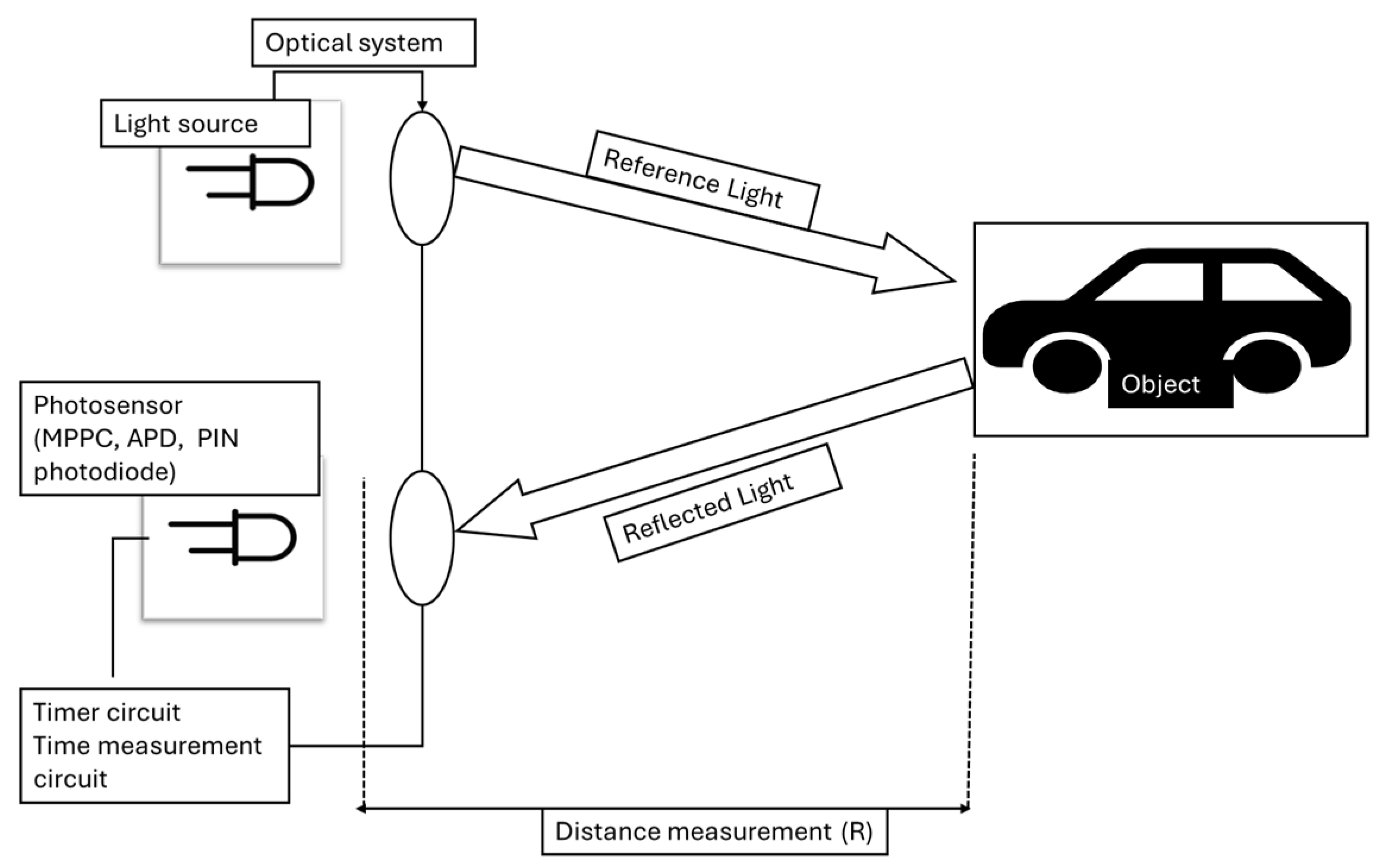
LIDAR operates by emitting a pulse of light in the infrared (IR) or near-infrared (NIR) spectrum from a laser diode. The emitted laser beam was split into two separate paths using an optical system: one portion served as reference light, while the other was directed toward the target object. The light reflected from the object’s surface followed the same optical path back to the photodetector, which captured and recorded the detection time and intensity of the returning signal, providing information about the object’s position. Once emitted, the laser pulse propagated for a specific duration (τ), triggering an internal clock within the timing circuit. The time difference ($∆\mathrm{t})$ between the reference light and the reflected signal was then used to accurately determine the object’s distance (R) from the LIDAR sensor using Equation (1) [17]. In this context, the intensity of the laser pulse (which is influenced by surface reflectivity and atmospheric conditions) was modeled using Equation (1). Meanwhile, the distance calculation, based on the time-of-flight (ToF) principle, is formulated in Equation (2) [17].

$$\mathrm{P}\left(\mathrm{R}\right)={\mathrm{P}}_0\rho {\displaystyle \frac{{\mathrm{A}}_0}{\pi {\mathrm{R}}^2}}{\mu }_0\cos \left(\theta \right){\mathrm{e}}^{-2\gamma \mathrm{R}}$$

(1)

$$\mathrm{R}={\displaystyle \frac{1}{2\mathrm{n}}}\mathrm{c}∆\mathrm{t}$$

(2)

Here, ${\mathrm{P}}_0$ represents the optical peak power of the emitted laser pulse,$\rho$ is the reflectivity coefficient of the target, ${\mathrm{A}}_0$ denotes the aperture area of the receiver, ${\mu }_0$ corresponds to the spectral transmittance of the detection optics, $\gamma$ represents the atmospheric extinction coefficient, $\mathrm{c}$ is the speed of light in a vacuum, $\theta$ is the angle of incidence of the laser beam on the surface, and $\mathrm{n}$ denotes the refractive index of the propagation medium (approximately 1 for air). A visual representation of these processes is shown in Figure 1.

This study focuses on laser intensity values and examines the influence of the optical properties of the target surface and distance of their determination. In this context, the fundamental LIDAR equation, presented in Equation (1), was utilized to model the energy loss and reflection effects of the laser pulse.

2.2. LIDAR Performance Metrics

In LIDAR systems, NPC and intensity are the key metrics used for performance evaluation. NPC represents the number of valid points obtained during a single scan cycle, providing insights into the spatial resolution and data density of the scanned area. Environmental factors and scanning parameters can significantly influence NPC values [18].

In this study, laser intensity is considered a key parameter for performance evaluation. Intensity represents the optical power of the laser light that is reflected from the target surface and detected by the LIDAR sensor. The returning laser signal was captured by photodetectors and converted into an electric current. This current was subsequently transformed into voltage by a transimpedance circuit, amplified, and transmitted to the LIDAR central control unit. Within the control unit, a digitization process normalized the intensity value within the 0–255 range for each laser pulse. This value serves as a direct indicator of both the surface reflectivity and the power of the laser light.

Laser intensity varies as a function of the optical properties of the target surface, laser geometry, and environmental conditions. Among these, surface reflectivity plays a critical role in determining laser intensity. Reflectivity quantifies how efficiently a surface reflects incident laser light and is influenced by physical factors such as material composition, color, and surface roughness. The color of a vehicle’s surface is one of the most crucial optical parameters affecting the accuracy of laser intensity measurements [19].

This study conducts a comprehensive analysis of the impact of vehicle surface color and reflectivity on laser intensity. Understanding the interplay between vehicle surface characteristics and laser intensity is essential for enhancing LIDAR sensor performance and optimizing environmental perception capabilities.

2.3. Experimental Data Sources and Collection

The study conducted by Shung et al. provides key findings that serve as a foundation for this research by systematically investigating the effects of automotive paints and environmental conditions on LIDAR performance. This study conducted a comprehensive analysis of the detectability of automotive paints with different colors and surface properties using intensity data obtained from LIDAR sensors. In the experimental setup, seven distinct automotive paint panels with matte black, gloss black, gloss white, gloss red, gloss blue, gloss silver, and gloss green finishes were employed. Each panel was further classified into metallic and non-metallic surfaces to examine the impact of surface composition on LIDAR reflectivity.

Table 1. SB/Standard black—black paint with standard black pigment.

No.	Color	Surface Finish	Panel Code
1	White	Gloss	SW-Gloss
2	Black	Gloss	SB-Gloss
3	Black	Matte	SB-Matt
4	Blue	Gloss	CDSBL-Gloss
5	Red (Metallic)	Gloss	TCSRM-Gloss
6	Green	Gloss	SMRTG-Gloss
7	Silver (Metallic)	Gloss	TSSM-Gloss

presents the colors and corresponding surface codes of the painted panels used in the tests [6].

The panels were coated using a manual spraying technique on flat, square nickel-plated mild steel plates. Each panel measured 50 cm × 50 cm, and, for larger surface tests, four panels were combined to create a 1 m × 1 m test surface. These dimensions were selected in accordance with physical constraints, and magnetic stabilizers were utilized to ensure precise panel positioning. During the experiments, the panels were oriented at different angles relative to the LIDAR sensor. Figure 2 illustrates the experimental setup used in this study, where a LiDAR sensor measures the reflectivity of test panels under controlled conditions. A customized mounting system ensures precise alignment and allows for systematic variation of panel angles between 0° and 70° in 5° increments. A digital angle gauge was used to ensure accurate angle adjustments. Additionally, reference surfaces, including matte black paper and a whiteboard, were incorporated to provide comparative reflectivity measurements. An alignment mirror was also utilized to maintain the sensor’s alignment with the center of the panel, ensuring consistency in data collection [6].

The Velodyne VLS-128 LIDAR (San Jose, CA, USA) sensor was utilized in this study. This sensor offers a detection range of up to 245 m with an accuracy of ±3 cm. It provides a total vertical field of view (FoV) of 40°, spanning from −25° to +15°, with a fine vertical angular resolution of 0.11°. Horizontally, it features a 360° FoV with an azimuthal angular resolution varying between 0.1° and 0.4°. The device operates at a wavelength of 903 nm and emits 0.39 mW of power per laser, adhering to Class 1 laser safety standards. The Velodyne VLS-128 acquires approximately 2,400,000 data points per second in single rotation mode, while this capacity increases to 4,800,000 points in double rotation mode. In this study, the device was configured to operate in single rotation mode, capturing only the first return of the laser beams. This approach facilitated faster and more efficient data processing. During testing, the sensor was operated at a rotation rate of 10 Hz, ensuring reliable intensity measurements across different distances [20].

2.4. Data Preparation and Processing

2.4.1. Experiment Data Preparation

In this study, the laser intensity data obtained from the study conducted by Shung et al. were digitized using computer-aided software. The extracted data were saved in CSV format and imported into Matlab R2021b for further processing. To ensure consistency and integrity, the Piecewise Cubic Hermite Interpolation (PCHIP) method was applied during the reconstruction of missing data points and the generation of standardized datasets of equal length for each graph. This method preserves the monotonicity between data points, providing a more natural transition while minimizing errors that may arise from linear interpolation [21].

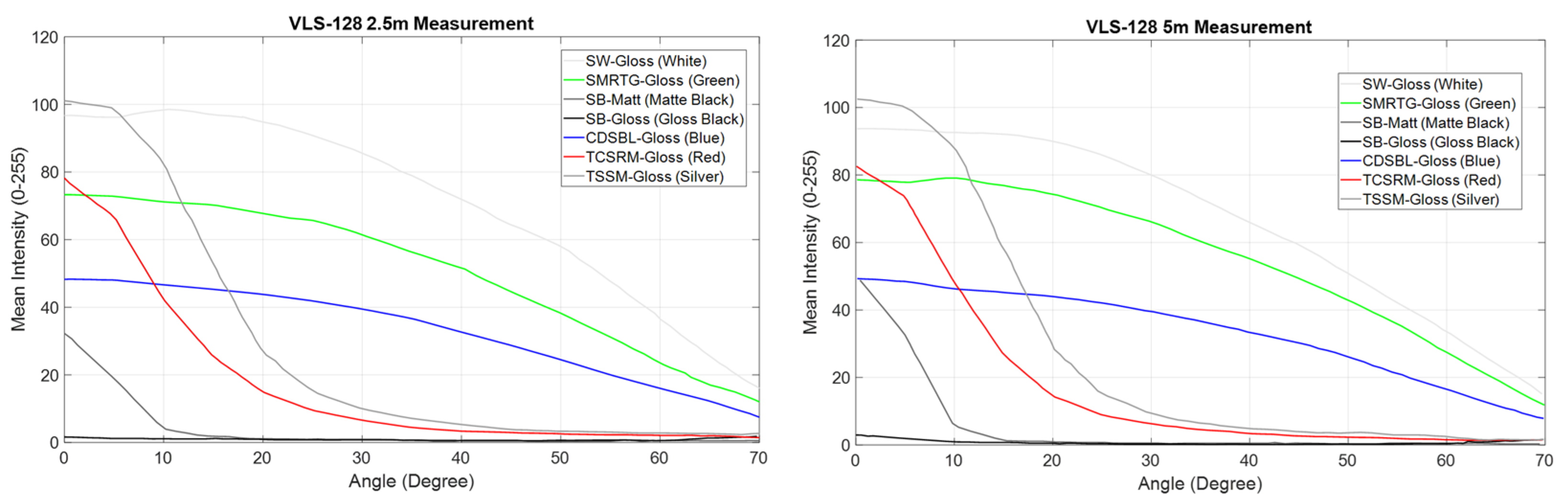
At the final stage of data processing, the datasets comprising angle, distance, and laser intensity values were standardized to contain 85 equally spaced data points for each parameter. This standardization ensured that laser intensity data collected at different distances and angles could be analyzed in a consistent and comparable format. In this study, laser intensity values were examined for four distinct distances: 2.5 m, 5 m, 10 m, and 30 m. At each distance, the influence of surface color on laser intensity was analyzed across incidence angles ranging from 0° to 70°. Figure 3 and Figure 4 illustrate the impact of color and surface characteristics on laser intensity values at these four distances.

The data indicate that laser intensity exhibits a complex relationship with surface reflectivity, angle, and distance. While, theoretically, laser power is expected to decrease inversely with the square of the distance, experimental findings did not fully align with this expectation. These discrepancies were attributed to factors such as the optical gain settings of the LIDAR sensor, the multi-channel structure, the divergence effect of laser light, and specular reflection [20].

At short distances, the SW-Gloss surface exhibited the highest laser intensity values, which can be attributed to the homogeneous reflection of laser light by glossy surfaces. In contrast, metallic surfaces such as TCSRM-Gloss displayed higher intensity values at low angles due to specular reflection; however, these values declined rapidly as the angle increased. Conversely, homogeneous reflective surfaces such as SW-Gloss demonstrated more stable laser intensity values despite angular variations. This finding suggests that, while metallic surfaces offer a sensor-oriented advantage at low angles, this effect diminishes as the angle increases. As distance increases, the divergence effect causes laser light to spread over a larger area. However, the multi-channel structure of the LIDAR sensor can compensate for this effect on measurements. For instance, at a distance of 30 m, the intensity values of the SMRTG-Gloss surface approached those of SW-Gloss, which can be explained by the laser light being collected from a broader area on uniformly reflective surfaces. Specular reflection decreases with increasing distance, leading to significant changes in laser intensity values. Notably, the high intensity values observed at low angles on metallic surfaces diminish with increasing distance, and the scattering of laser light in multiple directions accelerates this reduction. Conversely, glossy surfaces provide homogeneous reflection, resulting in more stable laser intensity values regardless of distance. These findings underscore the critical role of design and calibration processes in enhancing LIDAR sensor reliability and understanding their sensitivity to environmental conditions. In particular, the unexpected increases observed in laser intensity values at specific distances reflect the stabilizing influence of LIDAR’s multi-channel structure on measurements.

In the study conducted by Shung et al., both indoor and outdoor tests were conducted to investigate the impact of environmental conditions on laser intensity measurements. The outdoor tests aimed to assess the effects of atmospheric factors such as sunlight, wind, and other environmental influences on laser intensity. These tests were performed in an open field measuring 25 m × 5.5 m, where measurements were taken using three different panel types (SW-Gloss, SB-Gloss, and SB-Matt) at varying distances. The study reported that, while both indoor and outdoor measurements exhibited similar trends in laser intensity values, the intensity values recorded in indoor tests were higher due to the absence of atmospheric effects. This difference was attributed to the fact that indoor measurements serve as a reference dataset, free from environmental interference, thereby providing a controlled experimental baseline [6].

Although measurements were conducted at different distances and for various colors in the open-field tests, this article provides detailed results only for the indoor and outdoor measurements of the SW-Gloss surface at a distance of 10 m. This study observed a consistent ratio between indoor and outdoor intensity values for the SW-Gloss surface and assumed that this ratio could also be applicable to other surfaces and distances. Based on the data presented in this study, the relationship between laser intensity values in indoor and outdoor conditions was generalized for different distances and surface colors. Figure 5a illustrates the indoor and outdoor measurements for the SW-Gloss surface at a distance of 10 m, while Figure 5b presents the corresponding intensity ratios between these two conditions. This ratio was utilized as a scaling coefficient to adjust the indoor laser intensity data to match outdoor conditions. This generalization was made based on the findings of Shung et al., which indicated that similar trends were observed across different surfaces and distances. The derived coefficients were determined for use in the analysis and modeling of laser intensity values.

The reflectivity coefficient values for the paint colors used in this study were based on optical properties obtained from sources such as NASA ECOSTRESS [22], USGS High Resolution Spectral Library [23], Blazek et al.’s study [13], Levinson et al.’s study [24], and Kim et al.’s review [12]. However, since the exact specifications of the paints used in the experiments are not known, reflectivity coefficients were determined based on the properties of the pigments and materials commonly used for these colors in the automotive industry. This approach ensured that the reflectivity coefficient values obtained were consistent with real-world applications. In the automotive industry, paint pigments play a critical role in the aesthetic appearance and durability of vehicles. Generally, the pigments used have a dual function in terms of providing coloring and protective properties [24].

Table 2. Reflectivity coefficient values of different colors of paint panels used in the experiments.

No.	Color	Surface Finish	Reflectivity Coefficient (903 nm)
1	White	Gloss	0.9
2	Black	Gloss	0.05
3	Black	Matte	0.21
4	Blue	Gloss	0.35
5	Red (Metallic)	Gloss	0.5
6	Green	Gloss	0.44
7	Silver (Metallic)	Gloss	0.60

provides details of these key parameters used to analyze the effects of different paint colors on laser intensity.

2.4.2. Training and Optimization of the Model

In this study, six different models (Gaussian Process Regression (GPR), Polynomial Regression, Support Vector Machine (SVM), Decision Tree, Random Forest, and Gradient Boosting) were analyzed for predicting laser intensity values. The performance of these models was assessed using Root Mean Squared Error (RMSE) and R² (R-squared) metrics. RMSE quantifies the magnitude of the differences between the predicted and actual values, while R² measures the explanatory power of the model, indicating how well it accounts for the variability in the dataset.

The model inputs were derived from the data detailed in Section 2.4.1, ensuring consistency with the theoretical framework. In this context, the cosine of the angle, 1/R², reflectivity, and intensity values were used as input variables. To ensure a reliable evaluation of model performance, the K-Fold Cross-Validation method was employed. This technique involves dividing the dataset into equally sized subsets (folds). In each iteration, one subset was designated as the test set, while the remaining subsets were used for model training. K-Fold Cross-Validation ensures the efficient utilization of the entire dataset for both training and testing while reducing the risks of overfitting and underfitting. This process was repeated five times in total. A 5-fold cross-validation is widely preferred in the literature for small to medium-sized datasets, as it provides a balanced distribution between training and test data [25,26].

K-Fold Cross-Validation enabled the efficient utilization of the entire dataset for both training and testing while mitigating the risks of overfitting and underfitting. Additionally, this method facilitated the incorporation of limited observations into the model selection process, ensuring a more comprehensive evaluation. At the end of each iteration, RMSE, R², and Relative Error values were recorded, and the overall model performance was evaluated by averaging these metrics. While RMSE and R² measure absolute error and model explanatory power, Relative Error expresses the proportional error between the predicted and actual values as a percentage. The mean values of these performance metrics for each model are presented in

Table 3. K-Fold Cross-Validation performance values for the models examined.

Model	Mean RMSE	Mean R-Squared	Mean Relative Error (%)
GPR	0.83162	0.99245	8.852
Polynomial Regression	252.056	0.29727	947.620
SVM	204.918	0.52893	620.980
Decision Tree	26.274	0.99164	14.070
Random Forest	112.436	0.86051	281.790
Gradient Boosting	21.294	0.9937	39.615

.

The results clearly demonstrate that the GPR model outperforms other models in terms of RMSE, R², and Relative Error. This success is attributed to its ability to model complex and nonlinear relationships in small and dense datasets. Gaussian Process Regression (GPR) is a probabilistic regression method that models relationships between input and output variables using a statistical approach while incorporating uncertainty estimates in its predictions. Its effectiveness in high-dimensional and nonlinear data structures, enabled through kernel functions, makes GPR particularly well suited for small and noisy datasets [27]. In this study, the limited size of the dataset, the nonlinear relationships between distance, angle, and laser intensity, and the complex interactions among the analyzed variables are key factors contributing to the superior performance of the GPR model. The literature also highlights that GPR provides stable predictions with low error rates in small datasets [28]. Specifically, in cases where other models struggle to learn complex relationships or face the risk of overfitting, the kernel-based structure of GPR and its ability to compute statistical uncertainty make it the most effective solution for laser intensity prediction. Furthermore, the ability to directly estimate uncertainty in the model’s outputs positions GPR as a more reliable modeling approach, especially in applications such as LIDAR data analysis, where measurement accuracy is critical.

To enhance the performance of the GPR model and increase prediction accuracy, a hyperparameter optimization process was conducted. In this study, the kernel function was fixed as a squared exponential, while the optimal values of other hyperparameters (e.g., sigma and noise level) were determined using Bayesian optimization. The squared exponential kernel function offers significant advantages for modeling continuous and nonlinear data, such as laser intensity values. This function was specifically chosen because it facilitates the smooth and precise modeling of laser intensity variations across different distances and angles.

Bayesian optimization is widely recognized as an effective method when evaluating an objective function with a high computational cost. In this process, Expected Improvement (EI) and Upper Confidence Bound (UCB) acquisition functions were employed. EI is designed to select hyperparameters that are most likely to enhance model performance, whereas UCB ensures an optimal trade-off between exploration and exploitation. In this study, a value of K = 2 was chosen for UCB and retained as the default setting in Matlab. This selection provides an optimal balance between reliability and performance. Figure 6 illustrates the minimization of the objective function over multiple iterations in the Bayesian optimization process. In this figure, the blue color denotes the lowest RMSE values obtained through direct observations, while the green color represents the lowest RMSE values estimated by the Bayesian model.

The observed and predicted values show a significant decline over the iterations of the Bayesian optimization, demonstrating that the optimization process effectively enhances performance. The optimal value for the sigma hyperparameter was determined as 0.77256 using the Bayesian model prediction and 0.68476 through direct observations. The discrepancy between these two values stems from the Bayesian model’s capability to account for uncertain regions within the hyperparameter space. This characteristic enhances the generalization capacity of the model without negatively affecting its performance. Additionally, both values exhibit a plateau particularly between iterations 8, 9, and 10, indicating that Bayesian optimization has reached convergence, where the objective function attains its minimum value and further improvements become challenging. This confirms that the optimization process has been carried out in a stable and successful manner.

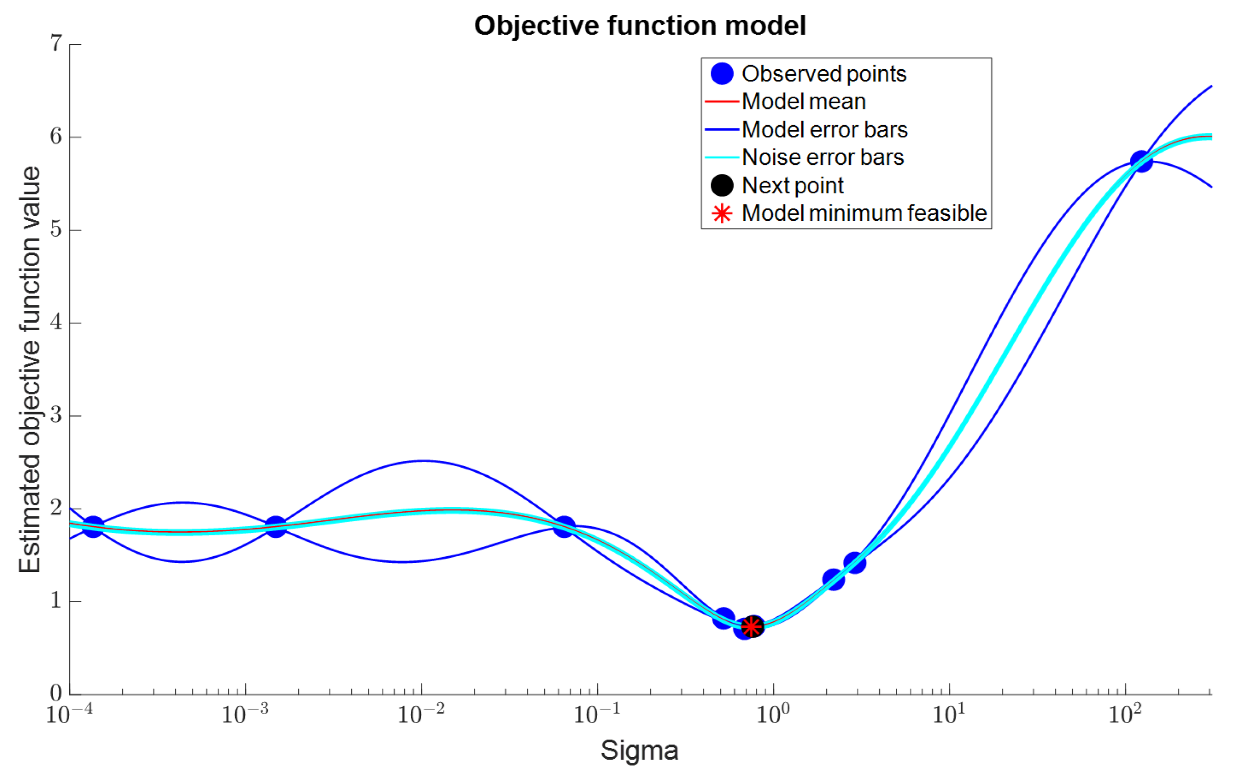
Figure 7 illustrates the solution space for the Sigma hyperparameter and its correlation with the objective function (RMSE). The figure depicts the predictions made for Sigma values during the Bayesian optimization process, along with the observed results of the objective function for these values. Here, the blue markers represent the Sigma values recorded during Bayesian optimization and their corresponding RMSE results. The red markers denote the average RMSE values predicted by the model for Sigma, while the error bars indicate the estimated uncertainty range and the impact of natural noise in the dataset.

Bayesian optimization effectively identifies uncertain regions in the hyperparameter space and determines optimal solutions for these areas. The graph indicates that, when Sigma is approximately 10⁻¹, the objective function reaches its minimum value. At this point, further improvements in model performance were not observed, and the objective function remained stable. This confirms that Bayesian optimization conducted a sufficiently thorough exploration of the solution space. As a result, the Bayesian optimization process successfully determined the optimal value of Sigma and minimized the objective function, thereby enhancing model performance.

Figure 8 illustrates the linear correlation between the laser intensity values predicted by the GPR model—optimized using the hyperparameters derived from the Bayesian optimization process—and the actual intensity values. Here, the blue circles represent the comparison between the predicted and actual values for each data point, while the linear trend of the slope clearly demonstrates the model’s high predictive accuracy.

The prediction accuracy of the optimized GPR model was evaluated using the obtained hyperparameters. Analysis of the model’s performance metrics revealed that the average RMSE value decreased from 0.87451 to 0.83162, while the average R² value increased from 0.99245 to 0.99924. These results indicate that the model is capable of predicting actual intensity values with very high accuracy. The reduction in RMSE confirms that the model significantly minimizes prediction errors, while the increase in R² demonstrates that the model explains a larger proportion of the variance in the dataset. These enhancements clearly highlight the effectiveness of the Bayesian optimization process in improving the performance of the GPR model.

In conclusion, the hyperparameter optimization process enhanced the laser intensity estimation performance of the GPR model. Bayesian optimization iteratively explored uncertain regions in the hyperparameter space, minimizing suboptimal or incorrect parameter selections. This process significantly improved the model’s capacity. Selecting the optimal hyperparameters enhanced the model’s prediction accuracy, mitigated the risk of overfitting, and strengthened its generalization ability. These findings underscore the effectiveness of the GPR model and emphasize the critical role of hyperparameter selection in Bayesian optimization.

2.4.3. Curve Fitting Methodology

To accurately analyze and integrate the data obtained from LIDAR sensors into the model, the measured intensity values must be correlated with the optical power reaching the detector. This relationship is derived from Equation (1), which represents the fundamental optical power equation of LIDAR. In LIDAR systems, the optical power reaching the detector exhibits a nonlinear dependence on distance, atmospheric absorption, reflectivity, and other environmental factors. Therefore, for precise analysis and modeling, intensity data must be transformed into physically meaningful quantities (e.g., optical power).

The intensity values obtained from LIDAR sensors are influenced by the characteristics of the sensor’s electronic and physical components. To establish a relationship between the digital data and the optical power reaching the detector, a transformation that accounts for the effects of these components (e.g., ADC, transimpedance amplifier, photodetector) is necessary. This transformation ensures that intensity values are converted into a physically consistent representation (e.g., optical power in Watts). The process of computing optical power from intensity values is described by Equation (3):

$${\mathrm{P}}_{\mathrm{o}\mathrm{p}\mathrm{t}\mathrm{i}\mathrm{c}\mathrm{a}\mathrm{l}}={\mathrm{I}}_{\mathrm{d}\mathrm{i}\mathrm{g}\mathrm{i}\mathrm{t}\mathrm{a}\mathrm{l}}{\displaystyle \frac{{\mathrm{V}}_{\mathrm{r}\mathrm{e}\mathrm{f}}}{2^{\mathrm{n}}-1}}{\displaystyle \frac{1}{{\mathrm{R}}_{\mathrm{f}}}}{\displaystyle \frac{1}{\mathrm{R}}}$$

(3)

Here, ${\mathrm{I}}_{\mathrm{d}\mathrm{i}\mathrm{g}\mathrm{i}\mathrm{t}\mathrm{a}\mathrm{l}}$ represents the digital output of the ADC (ranging 0–255), ${\mathrm{V}}_{\mathrm{r}\mathrm{e}\mathrm{f}}$ denotes the reference voltage of the ADC (3.3 V), n indicates the resolution of the ADC (8 bits), ${\mathrm{R}}_{\mathrm{f}}$ refers to the load resistance (1 $\mathrm{k}\Omega$) of the transimpedance amplifier responsible for current-to-voltage conversion. $\mathrm{R}$ (0.8 A/W) represents the sensitivity of the photodetector.

In the first step, the intensity values were converted into voltage using the reference voltage and resolution of the ADC. The resulting voltage was then converted into a current through the load resistance of the transimpedance amplifier and ultimately transformed into optical power, reaching the detector based on the sensitivity of the photodetector. Furthermore, LIDAR sensors typically collect data from multiple channels using detector arrays. In this study, the intensity measurements provided by the sensor represent a single data point, which corresponds to the average value across all channels. Therefore, the intensity values obtained from the LIDAR sensor were analyzed under the assumption that they reflect the mean intensity of all detector channels. This approach not only simplifies data processing but also aligns with the physical characteristics of the intensity data output by the LIDAR device used in the experimental setup. Curve fitting serves as a critical tool for aligning these intensity values with the fundamental LIDAR equations. These transformation and curve fitting processes play a key role in ensuring that LIDAR data are analyzed in accordance with physical principles and effectively utilized in modeling applications.

In this study, distance, angle, and reflectivity coefficient values were provided as input parameters to the GPR model. The same parameters were also applied as inputs to Equation (1), the fundamental optical power equation of LIDAR systems. This approach facilitated the derivation of a conversion function that links both theoretical and experimental data. The GPR model predicts intensity values based on the input parameters, and these predictions are converted into optical power values at the detector using Equation (3). Simultaneously, theoretical optical power values are computed using Equation (1). A curve fitting process was then applied between these two sets of optical power values to formulate a transformation equation that aligns the experimental intensity data with the theoretical optical power.

In this study, since LIDAR measurements were conducted in open fields of view, the atmospheric attenuation coefficient used in Equation (1) at a wavelength of 90 nm was set to γ = 0.01 m⁻¹ as determined by the Kim–Kruse model [29]. This coefficient represents the propagation and absorption effects of laser light in the atmosphere under open-air conditions. Additionally, in devices such as the VLS-128, the spectral transmittance of the detection optics is generally close to 1 at a wavelength of 903 nm. This allows the LIDAR-emitted laser light to be detected by the sensor with maximum efficiency, thereby enhancing the optical performance of the system. Therefore, the $\mu ₀$ value was taken as 1 in this study. Furthermore, an analysis of the relevant LIDAR datasheet was conducted to determine the receiver aperture area. It was found that the VLS-128 features a 12.4 cm² receiver aperture area for collecting laser reflections [30]. The receiver aperture area is a crucial parameter that directly influences the amount of laser power collected by the detector, thereby contributing to the overall sensitivity of the system. Accordingly, this parameter was incorporated into the analysis to ensure accurate modeling of LIDAR measurements.

The LIDAR system used in the experimental process operates under specific experimental conditions and technical limitations, as stated in the study conducted by Shung et al. Specifically, the laser power was set to 0.39 mW in compliance with the Class 1 laser safety standards of the respective LIDAR model. In the experimental setup, one side of the laser beam was completely blocked by a black panel, ensuring no reflections from this area. As a result, only 96 channels were considered active instead of the full 128 channels of the LIDAR. This adjustment means that reflections from the blocked region were excluded from the intensity data calculations.

In this analysis, the curve fitting process applied to the LIDAR data considered the sensitivity of vehicles to factors such as their distance from and angle to the sensor. Specifically, the vehicle angle relative to the sensor was assumed to be between 0° and 5° during this study. This assumption was made because vehicles detected by LIDAR under normal traffic conditions typically fall within a narrow angular range.

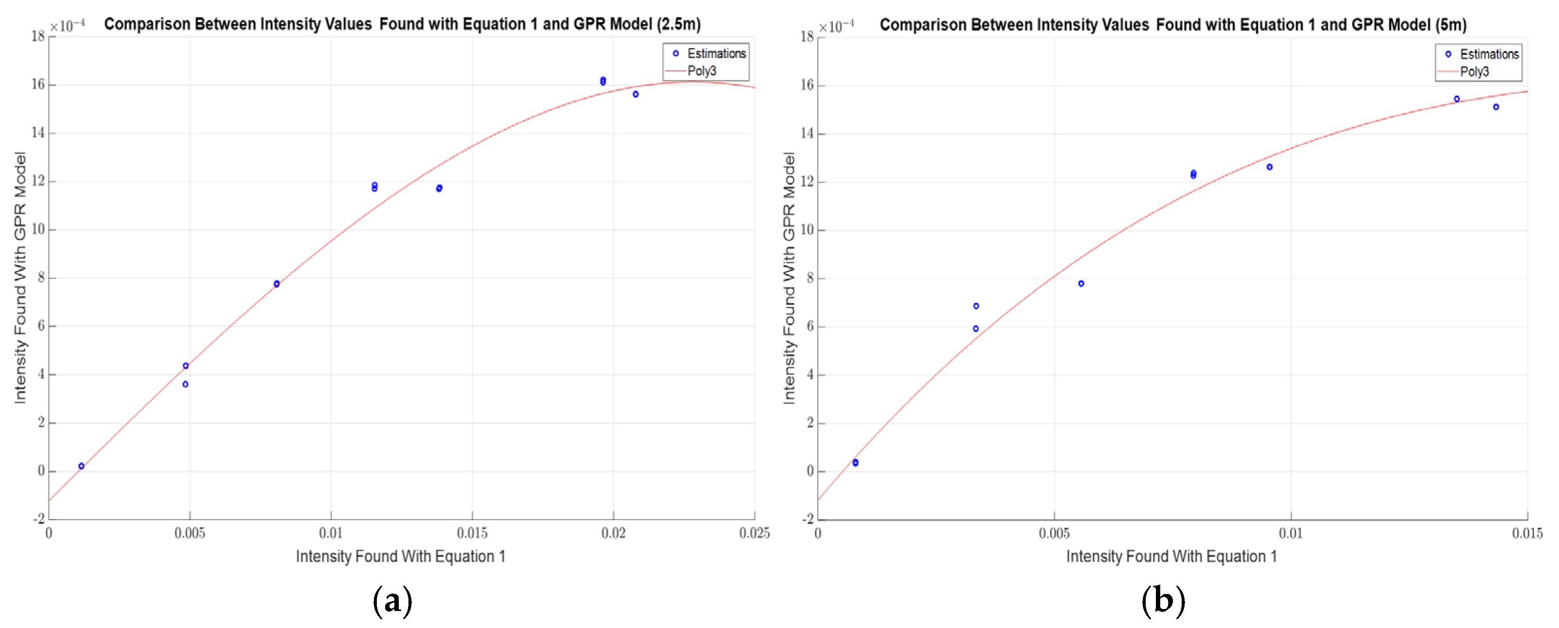
Furthermore, this study focused on LIDAR sensors’ ability to analyze vehicles passing in close proximity, particularly at distances of 2.5 m and 5 m. However, discrepancies between theoretical and experimental results were observed due to laser intensity attenuation, sensor optical gain settings, and environmental factors. Consequently, separate curve fitting processes were conducted for 2.5 m and 5 m distances. To enhance the representation of data at different distances, two distinct transformation equations were derived using a third-degree polynomial (poly3) function, as described in Equation (4). These equations were constructed by randomly selecting different reflectivity coefficients and angle values for each distance. This approach enabled the modeling of different scenarios and improved the accuracy of the fitting process.

$$\mathrm{P}\mathrm{o}\mathrm{l}\mathrm{y}\left(\mathrm{x}\right)={\mathrm{p}}_1{\mathrm{x}}^3+{\mathrm{p}}_2{\mathrm{x}}^2+{\mathrm{p}}_3\mathrm{x}+{\mathrm{p}}_4$$

(4)

First, the curve fitting process was conducted for a distance of 2.5 m. Figure 9 illustrates the curve fitting plots for 2.5 m and 5 m, depicting the relationship between Equation (1) and the intensity values predicted by the GPR model. In the figure, the red curve represents the third-degree polynomial (poly3) function used for curve fitting, while the blue dots correspond to the theoretical and experimental intensity values. The coefficients of the derived equations for each distance are presented in

Table 4. Equation coefficients derived from curve fitting for 2.5 m and 5 m distances.

Coefficient	$2.5 (\mathbf{m}$)	$5 (\mathbf{m}$)
p1	−34.52	−90.57
p2	−1.21	−5.092
p3	0.1229	0.2078
p4	0.0001231	−0.0001086

.

In conclusion, incorporating parameters such as distance, angle, and reflectivity into the model, both experimentally and theoretically, has played a crucial role in transforming intensity values into physically meaningful optical power values. The transformation equations derived from curve fitting have enabled a more realistic modeling of LIDAR measurements and have effectively supported the performance analysis of LIDAR sensors, aligning with the main objectives of this study.

2.5. Dataset Description

In this study, the CUPAC dataset, collected by Coventry University, was selected to assess the performance of the developed model under real-world conditions and to explore its potential applications in environmental sensing [16]. This dataset encompasses a diverse range of road, traffic, and weather conditions, making it a suitable testbed for modeling various environmental scenarios.

The characteristics of the LIDAR sensor played a decisive role in the selection of the dataset. The Velodyne VLP-16 LIDAR sensor used in the CUPAC dataset shares a similar technological foundation with the Velodyne VLS-128, which was employed in training the model in this study. Both sensors operate at a wavelength of 903 nm, are capable of measuring reflectivity, and comply with Class 1 laser safety standards. However, while the VLS-128 features a total of 128 channels and a combined laser power of 49.92 mW, the VLP-16 is equipped with only 16 channels and delivers a total laser power of 6.24 mW. This variation in laser power and channel count in the VLP-16 presents a significant advantage for this study. It enables an evaluation of the model’s applicability not only to high-resolution sensors like the VLS-128 but also to other LIDAR systems operating in similar modes, thereby demonstrating its broader usability.

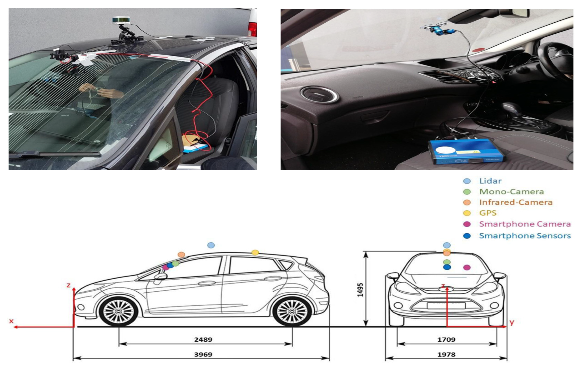
The data collected through monocular, infrared, and smartphone cameras, a LIDAR sensor, GPS receivers, smartphone sensors, and a CAN-Bus data logger integrated into the research vehicle were used to comprehensively analyze the interactions between the vehicle’s environmental perception and real-time responses. The CUPAC dataset was regulated under the General Data Protection Regulation (GDPR) to ensure ethical data processing. Video sequences recorded by the three-camera system were manually scanned for license plates and human faces and labeled using Matlab Ground Truth Labelers. The labeled regions were then blurred using a Gaussian filter. The equipment and sensors used in this study include a Racelogic VBOX video (Buckingham, UK) monocular camera (1920 × 1080 resolution/30 fps), Racelogic VBOX video HD2, CAN-Bus data logger (10 Hz), GPS antenna (10 Hz), Velodyne VLP-16 LIDAR sensor (600 rpm/10 Hz), FLIR One Pro infrared camera (1080 × 1440 resolution/8–9 fps), and Samsung Galaxy S8 camera (1080 × 720 resolution/30 fps). The LIDAR unit, infrared camera, and GPS receiver were mounted outside the research vehicle, while the remaining sensors were positioned inside the vehicle. All these placement details, along with the vehicle dimensions and sensor positions, are shown together in Figure 10. However, the smartphone camera and sensors are not included in the figure.

The Velodyne VLP-16 used in the measurements is capable of producing high-resolution 3D LIDAR data points. This sensor features a 12.4 cm² receiver aperture area and a 16-channel structure, offering a measurement range of up to 100 m with a typical range accuracy of ±3 cm. It provides a vertical field of view (FoV) ranging from +15.0° to −15.0°, with a vertical angular resolution of 2.0°. Horizontally, it offers a 360° field of view, and the horizontal/azimuth angular resolution varies between 0.1° and 0.4°. The sensor’s rotation speed can be adjusted between 5 Hz and 20 Hz. In single rotation mode, it generates 300,000 LIDAR data points per second, while, in double rotation mode, this capacity increases to 600,000 points per second. During the data collection process, the sensor was operated at a 10 Hz rotation rate and in single rotation mode. The collected data, including distance measurements, reflectivity values, rotation angle, and timestamps, was transmitted via a 100 Mbps Ethernet connection [30].

Table 5. Dataset scenario summary.

No.	Time (min)	Traff. D.	Traff. P.	Weather	Time	Features
a1	6.4	High	High	Cloudy	Afternoon	Inner-city, Parking lot
a2	8.3	Low	High	Cloudy	Afternoon	Parking lot, Country road
a3	8.3	High	Low	Cloudy	Afternoon	Inner-city, Country road
a4	8.3	High	Medium	Cloudy	Afternoon	Inner-city
b1	6.28	Medium	Medium	Sunny	Noon	Inner-city
b2	16.92	Low	High	Sunny	Noon	Residential area, Road bumps
b3	25.38	Medium	High	Sunny	Noon	Residential area, Road bumps, Inner-city

presents the characteristics of each scenario, including traffic volume (Traff. D.) and parked vehicles (Traff. P.) recorded during driving, as well as weather conditions, time of day, and the key features defining each trial scenario.

The collected data were stored in .PCD format with a .pcd extension. This data structure includes the location (X, Y, Z coordinates), intensity, point count, and coordinate limits (XLimits, YLimits, ZLimits) for each point. The point cloud dataset has a dimension of 16 × 1808, providing detailed three-dimensional positional information and intensity values for each point. This structure enables the analysis and visualization of environmental data captured by the LIDAR sensor.

2.6. Evaluation of Model Performance Using Real-World Data

In this section, measurements and scenarios from the CUPAC dataset were analyzed to evaluate the performance of the developed model during real driving conditions. Additionally, this analysis aimed to assess the model’s performance on a different LIDAR device. In the dataset, only vehicle scenarios corresponding to the color charts used in this study were examined. To prevent environmental effects from being incorporated into the model and to ensure that only vehicle-induced effects were included in the analysis, a spatial filtering process was applied. This filtering process selected only the points within specific x, y, and z boundaries where the vehicle was located. After filtering, the reconstructed PCD data were isolated from surrounding objects and ground effects. Additionally, in the study conducted by Shung et al., it was stated that the outdoor experiments were conducted in open-air conditions during the daytime. Therefore, when selecting appropriate scenarios from the CUPAC dataset, care was taken to ensure similar environmental conditions, and measurements conducted in open-air and daytime settings were preferred. Moreover, the CUPAC dataset does not include any labeling or information regarding the age of the vehicles. Similarly, in the study conducted by Shung et al., which was used as a reference for model training, there was no evaluation of the age of the test panels. For this reason, the effect of the age factor was omitted in this study [6,16].

To accurately analyze the data obtained from LIDAR measurements, the distance and angle between the vehicle and the sensor were calculated using trigonometric transformations based on three-dimensional coordinate data obtained after spatial filtering. In these calculations, both the vertical (ϕ) and horizontal (θ) angles were considered, and this information was provided as input parameters to the model. Furthermore, the role of the horizontal angle between the vehicle and the sensor in determining the effective laser channels was evaluated. The distance parameter was calculated using Equation (5), where x, y, and z represent the three-dimensional spatial coordinates of the vehicle relative to the sensor.

$$\mathrm{r}=\sqrt{{\mathrm{x}}^2+{\mathrm{y}}^2+{\mathrm{z}}^2}$$

(5)

The vertical angle (ϕ) defines the up/down axis orientation of the vehicle relative to the sensor and directly corresponds to the “angle” parameter in the model. The vertical angle was calculated using Equation (6).

$$\mathsf{\varphi }={\tan }^{-1}\left({\displaystyle \frac{\mathrm{z}}{\sqrt{{\mathrm{x}}^2+{\mathrm{y}}^2}}}\right)$$

(6)

The horizontal angle between the vehicle and the sensor determines the vehicle’s position within the sensor’s scanning field on the horizontal plane. This angle was calculated using Equation (7).

$$\theta ={\mathrm{t}\mathrm{a}\mathrm{n}}^{-1}\left({\displaystyle \frac{\mathrm{y}}{\mathrm{x}}}\right)$$

(7)

The calculations in Equations (5)–(7) were individually applied to all selected points, and the averaged values were used to determine the vehicle’s overall distance and angle relative to the sensor. The reference position of the LIDAR was obtained from the coordinates provided in the CUPAC dataset [16].

The 16 laser channels of the VLP-16 sensor, as specified in the datasheet, are positioned at vertical angles ranging from +15° to −15°. This configuration enables the sensor to fully scan the vertical position of the vehicle. The arrangement, in which all vertical laser channels can effectively capture the vehicle’s position, prevented data loss between the sensor and the vehicle while ensuring that all channels contribute to the measurements taken on the vehicle.

However, the specific position of the vehicle within the sensor’s horizontal scanning area allowed only the laser channels falling within this region to contribute to the measurements. In the VLP-16 sensor, each laser channel was positioned to perform a full 360° horizontal scan. However, since environmental effects are eliminated through spatial filtering, only the laser channels that intersect with the vehicle’s region during a measurement influence the intensity values. In this context, the effective number of laser channels (N) was calculated using Equation (8). This formula was employed to determine the effectiveness of the laser channels on the vehicle based on the horizontal angle between the vehicle and the sensor. The effective number of channels was utilized as an input parameter in the model.

$$\mathrm{N}={\displaystyle \frac{16}{360}}\theta$$

(8)

Finally, all invalid (NaN) values were removed from the filtered point cloud of the vehicle object, and the average intensity value was computed based on the selected points. This process ensured that only the effects originating from the vehicle were analyzed, allowing this study to be conducted with data free from environmental influences. The obtained average intensity value was then compared with the intensity value predicted by the model, which was based on the input parameters: distance, angle, color, and the number of active laser channels.

3. Results

In this section, the performance of the developed model was analyzed through a two-stage evaluation process. First, to assess the accuracy of the model and its consistency with the literature, it was evaluated using the input parameters proposed by Shung et al. and compared with reference values. This step aims to demonstrate that the model operates in alignment with existing methodologies in the literature and produces predictions consistent with the theoretical framework. In the second stage, the model’s performance under real-world traffic conditions was analyzed using the CUPAC dataset. Appropriate scenarios were selected, and spatial filtering was applied to eliminate environmental effects, ensuring that only laser intensity values originating from the vehicle object were analyzed. The distance between the vehicle and the sensor, along with vertical and horizontal angles and color information, were provided as input parameters to the model. The model’s predictions were then compared with actual measurement data. This evaluation process highlights the applicability and generalizability of the model to different LIDAR systems. Initially, the colors used in the study conducted by Shung et al. were analyzed at distances of 2.5 m and 5 m and at angles of 0° and 5°. These distance and angle ranges align with the constraints defined in the modeling process. The number of effective laser channels and other parameters were also adjusted to match the experimental conditions described in the original study.

Table 6. Comparison of the estimated intensity values obtained from the developed GPR and curve-fitting model with the actual intensity values reported by Shung et al. [6].

Color	Distance	Degree	Estimated	Real	Accuracy (%)
	$\left(\mathbf{m}\right)$	(°)	Intensity	Intensity
SW-Gloss (White)	2.5	0	97.660	96.714	99.629
		5	97.495	96.174	99.482
	5	0	95.561	93.715	99.276
		5	95.034	93.486	99.393
SB-Matte (Black)	2.5	0	30.109	32.238	99.165
		5	19.863	18.392	99.423
	5	0	45.632	48.838	98.743
		5	33.851	31.648	99.136
SB-Gloss (Black)	2.5	0	1.751	1.601	99.941
		5	1.274	1.173	99.960
	5	0	3.125	2.956	99.934
		5	1.962	1.840	99.952
CDSBL-Gloss (Blue)	2.5	0	48.727	48.224	99.803
		5	48.150	47.971	99.930
	5	0	50.015	49.295	99.713
		5	47.894	48.186	99.886
TCSRM-Gloss (Red)	2.5	0	74.861	78.191	98.694
		5	68.862	66.267	98.982
	5	0	80.277	82.602	99.088
		5	74.454	72.763	99.337
SMRTG-Gloss (Green)	2.5	0	75.349	73.268	99.184
		5	74.193	72.659	99.398
	5	0	81.113	78.602	99.015
		5	79.140	77.831	99.487
TSSM-Gloss (Silver)	2.5	0	99.930	101.064	99.555
		5	97.211	97.235	99.991
	5	0	100.827	102.497	99.345
		5	96.849	99.010	99.153

presents the predicted and actual intensity values, along with the percentage accuracy values, providing a quantitative assessment of the model’s accuracy.

As observed in the results, the predicted intensity values from the model exhibit a high level of agreement with the actual intensity values. The accuracy rates presented in Table 6 are consistently above 98%, demonstrating that the model performs reliably across different distances, angles, and surface types.

For a distance of 2.5 m and an angle of 0°, the highest accuracy was achieved on the SB-Gloss (Black) surface with 99.941%. The lowest accuracy under the same conditions was observed on the TCSRM-Gloss (Red) surface at 98.694%. The model’s consistent accuracy above 98% across all surfaces demonstrates its strong predictive performance, even on surfaces with varying reflectivity properties. For 2.5 m and 5°, the model maintained similarly high accuracy levels. The highest accuracy was recorded for the SB-Gloss (Black) surface at 99.960%, while the lowest accuracy was 98.982% for the TCSRM-Gloss (Red) surface. In this angular range, the model exhibited an accuracy above 99% for the other colors, highlighting its robustness against angular variations.

For a distance of 5 m and an angle of 0°, the model once again demonstrated strong performance, achieving the highest accuracy of 99.991% on the TSSM-Gloss (Silver) surface. The lowest accuracy was recorded at 99.015% for the SMRTG-Gloss (Green) surface. Despite the increased distance, the model maintained an accuracy above 99%, particularly for glossy and metallic surfaces, indicating its consistency in handling light reflectivity properties. For 5 m and 5°, the highest accuracy was observed on the SMRTG-Gloss (Green) surface at 99.487%, while the lowest accuracy was 99.153% on the TSSM-Gloss (Silver) surface. These accuracy levels demonstrate that, even at a distance of 5 m, the model maintains a highly stable prediction performance.

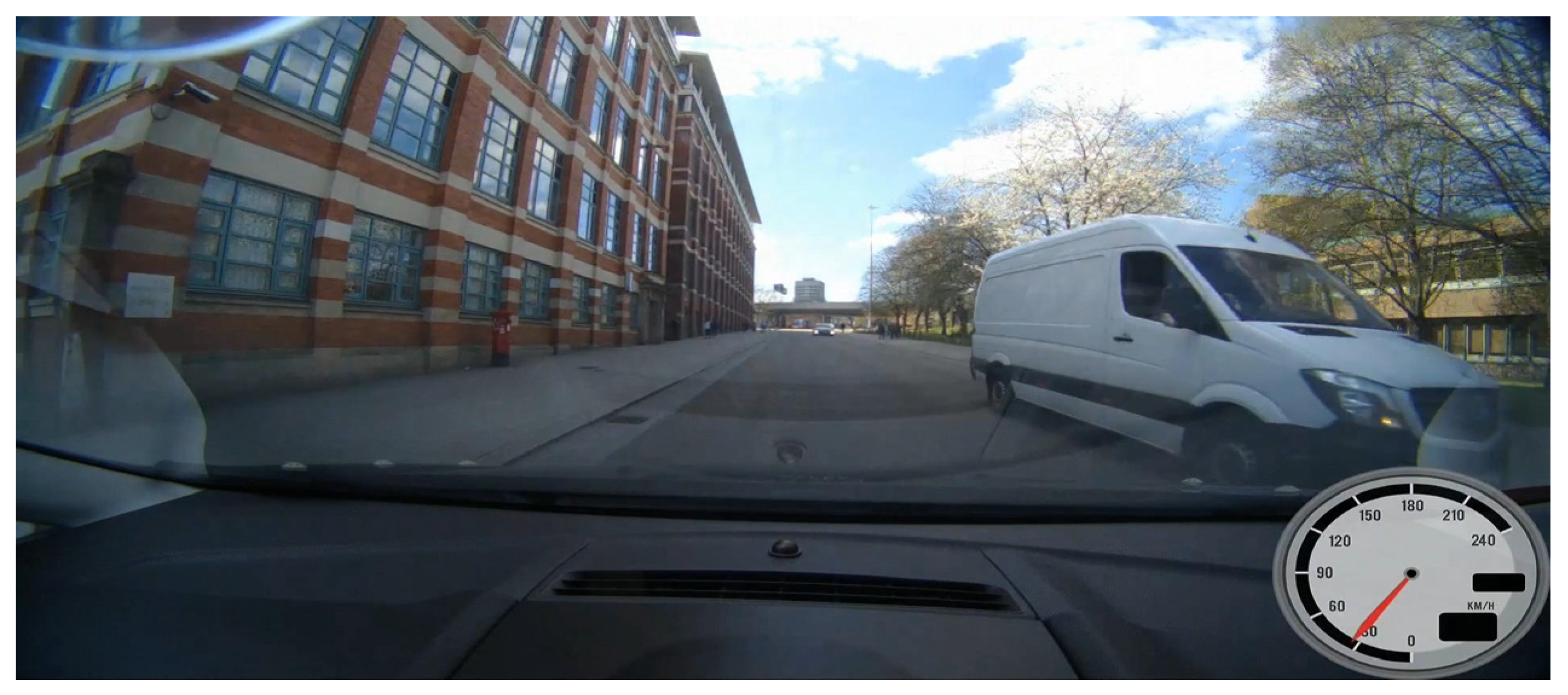
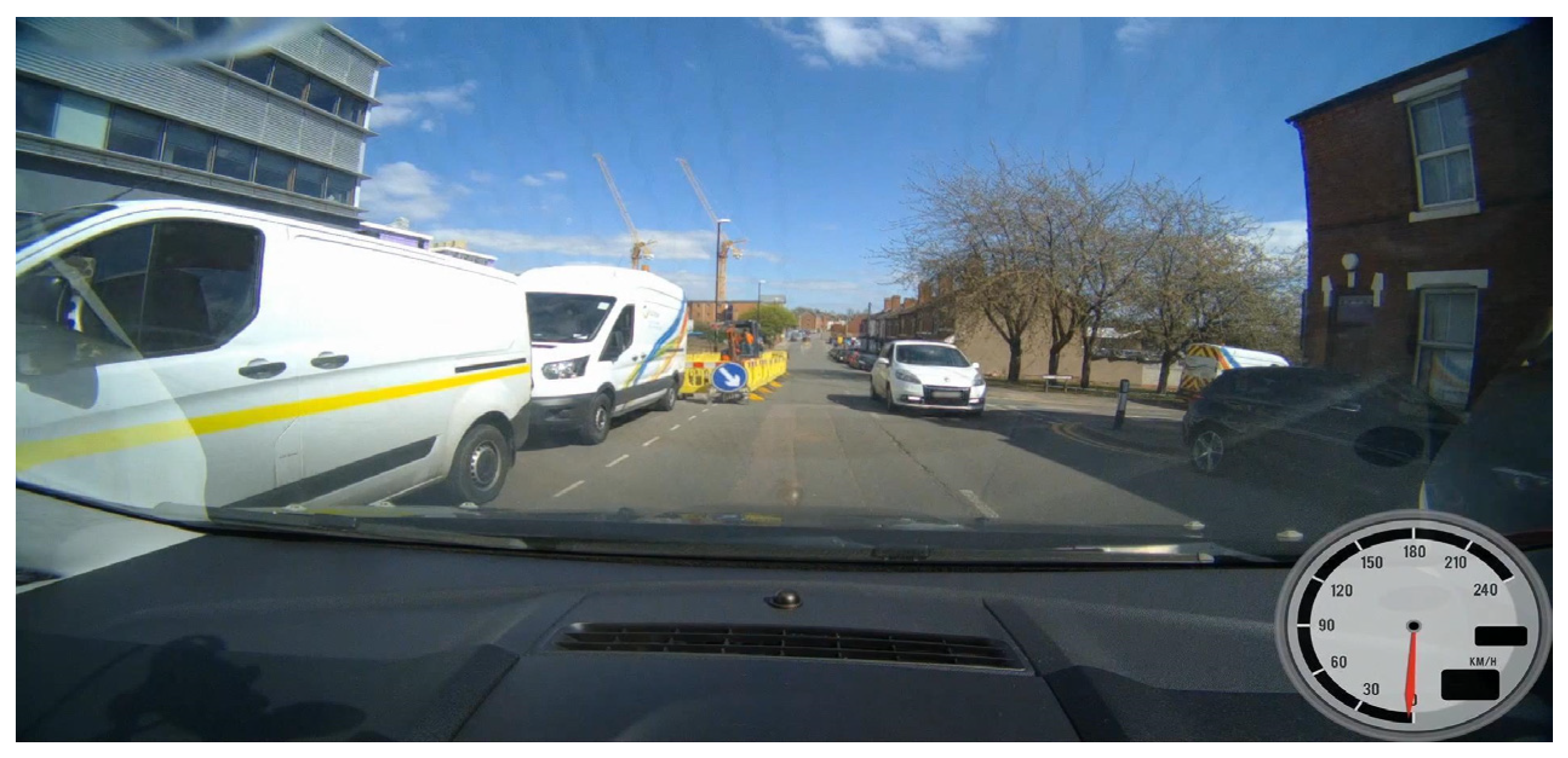
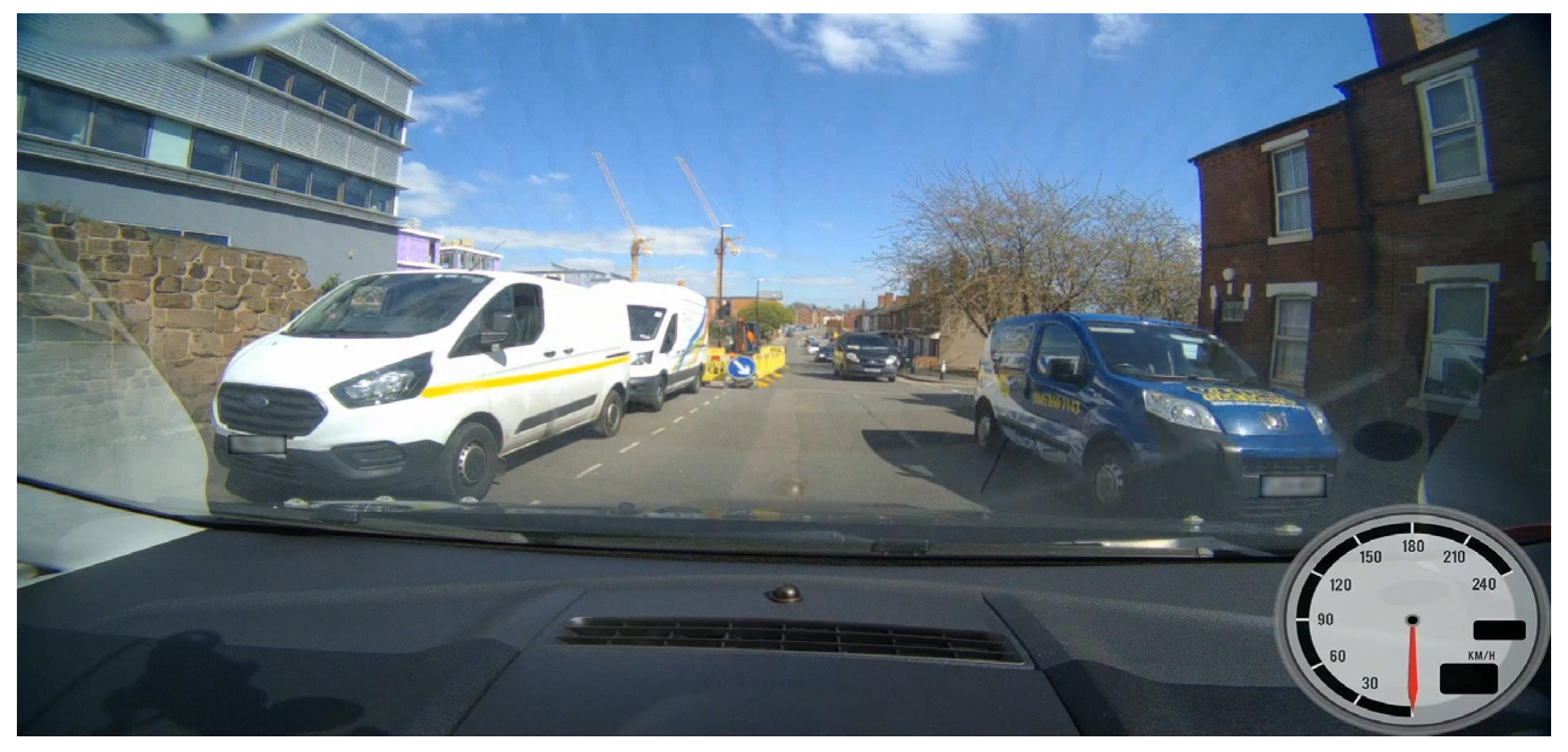
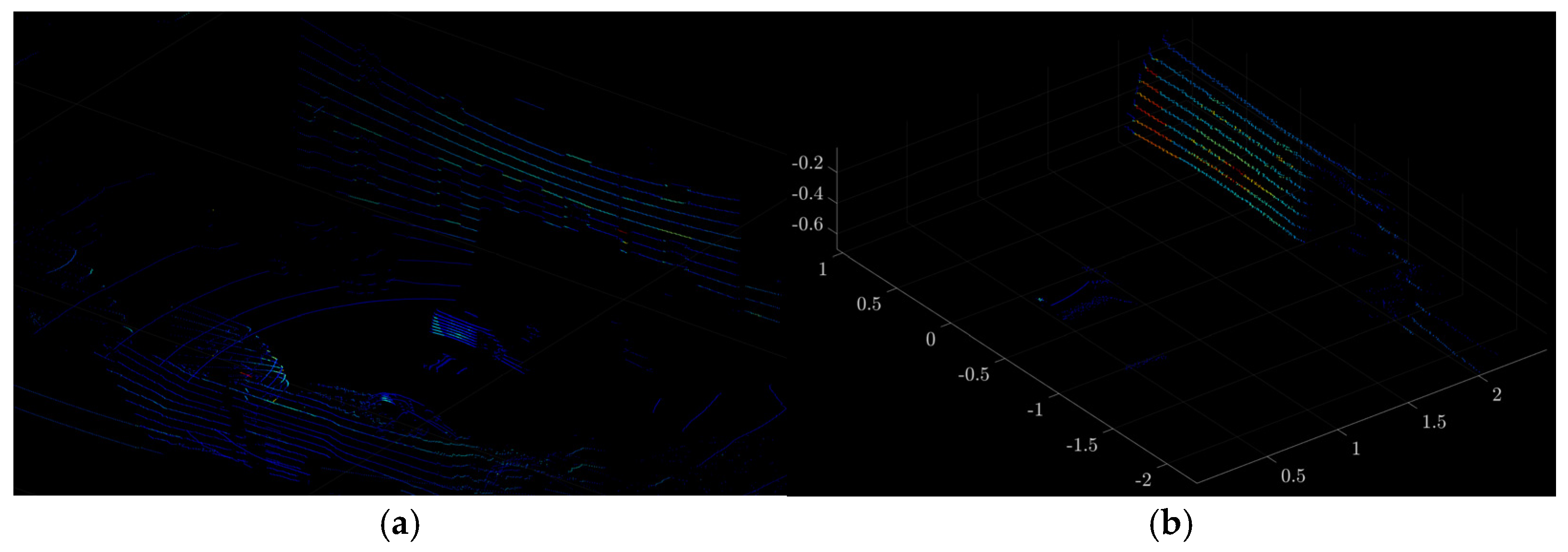
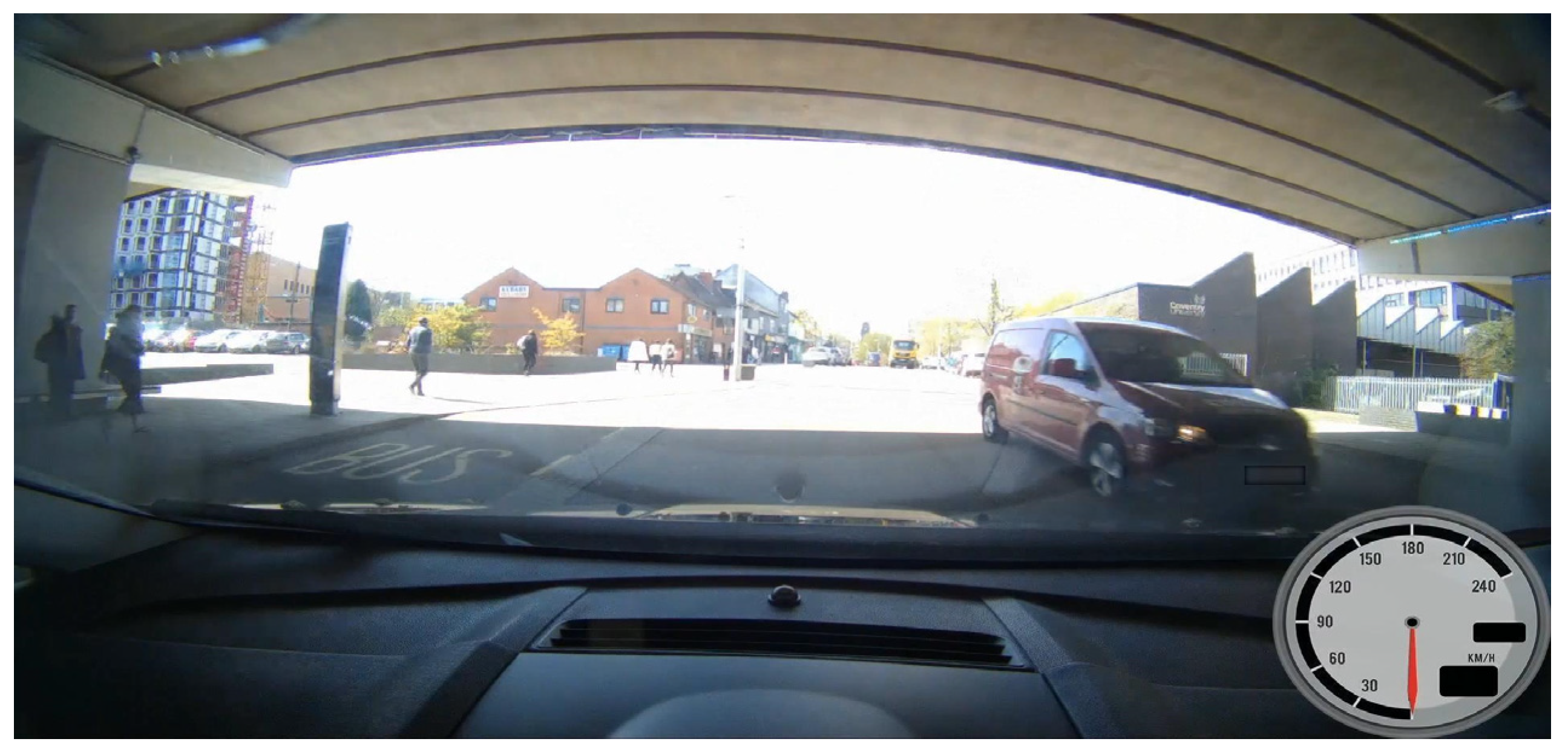
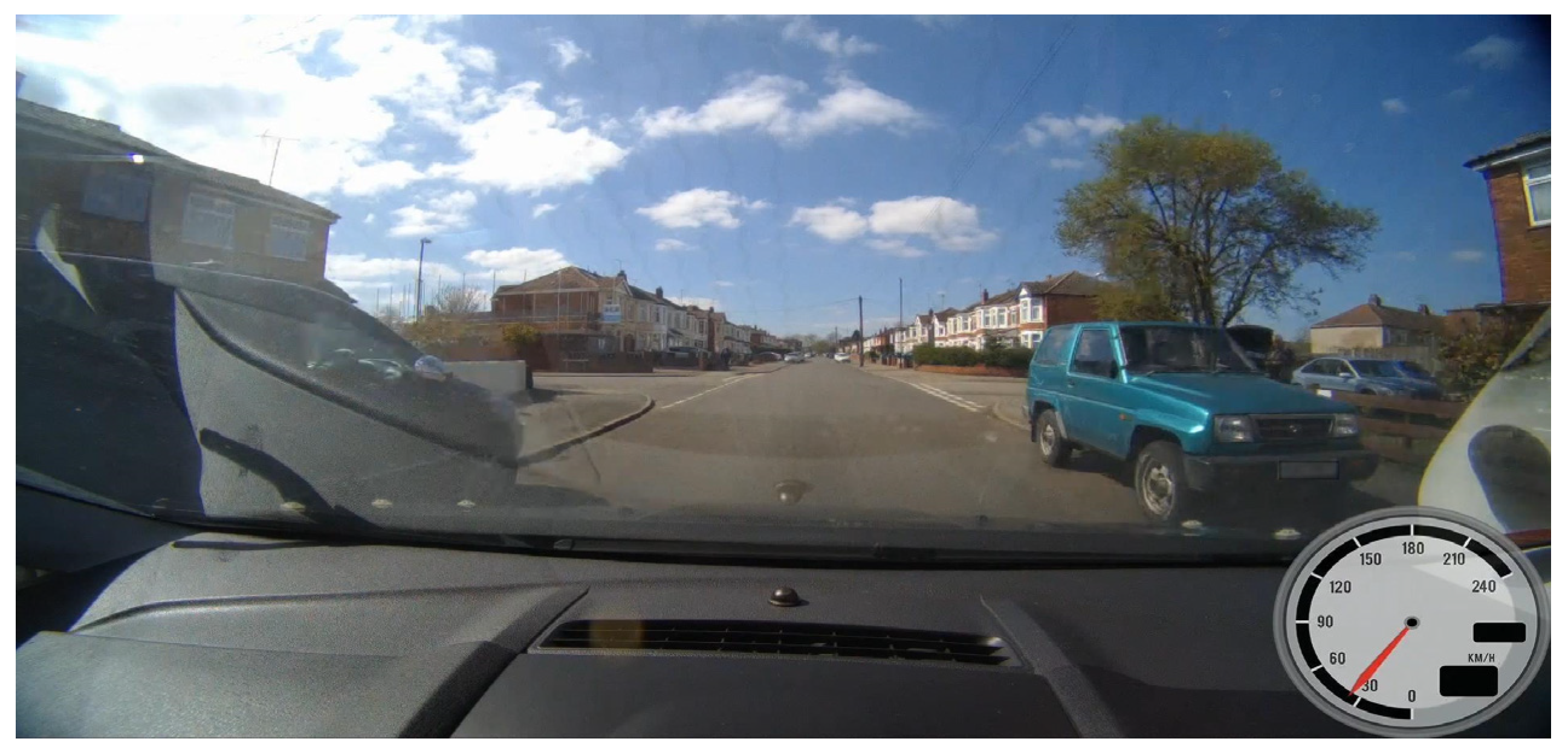
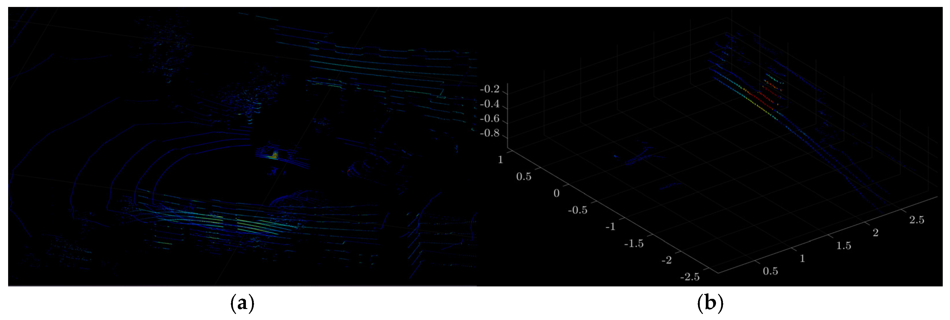
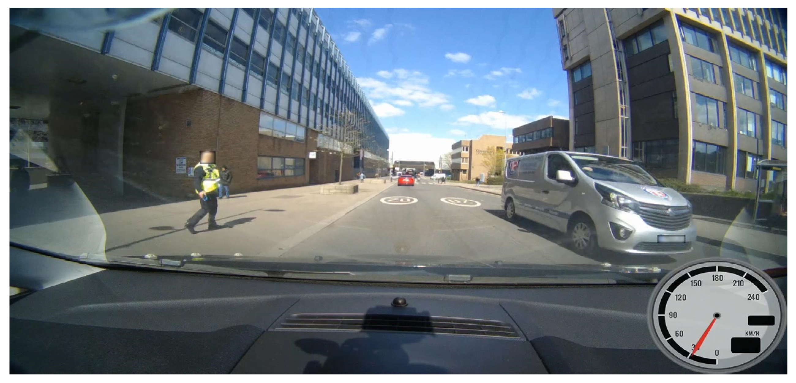
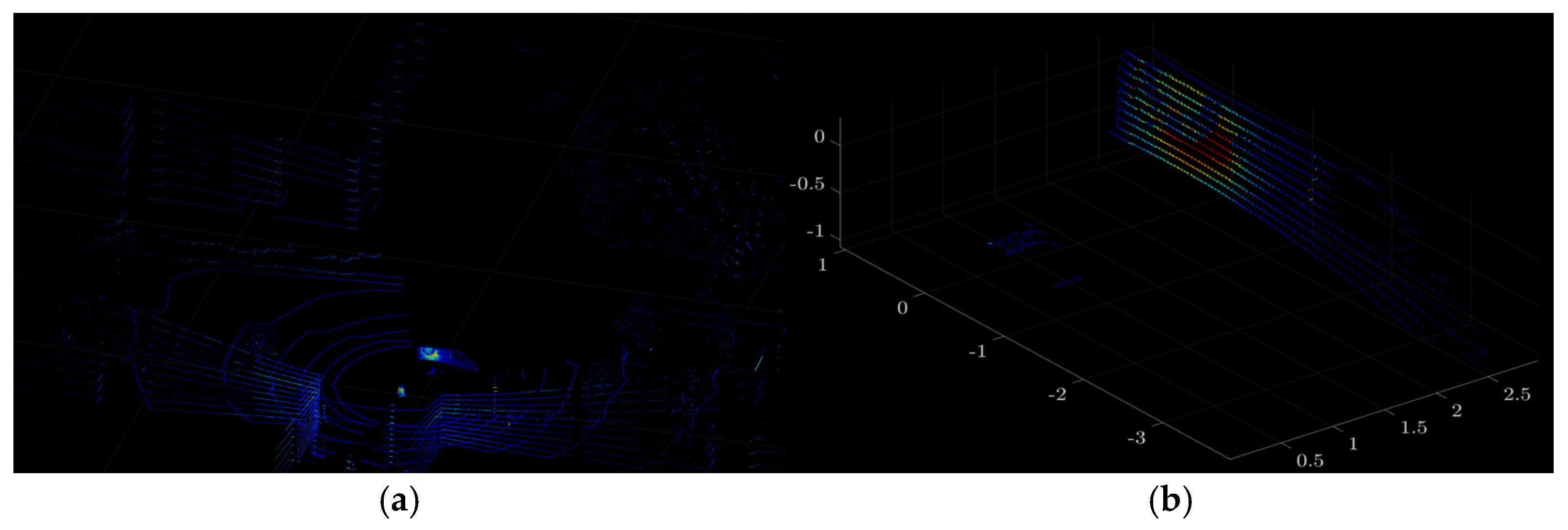
Seven different measurements from the CUPAC dataset were analyzed in detail to identify scenarios that match the vehicle colors examined in this study. First, the camera images corresponding to each measurement were reviewed, and the PCD data of the selected scenarios were processed in Matlab. During this process, the laser intensity distribution was visualized along with the vehicle’s position and surrounding objects. Subsequently, spatial filtering was applied to isolate laser reflections only from the vehicle’s surface, effectively eliminating the influence of surrounding objects on the measurements. As a result, only the laser intensity values reflected from the vehicle surface were obtained.

For each measurement, three different visualizations are provided: (i) the camera image corresponding to the measurement, (ii) the overall laser intensity distribution including the vehicle and its surroundings, and (iii) the point cloud containing only the laser intensity values of the vehicle after spatial filtering. These visualizations are presented in Figure 11, Figure 12, Figure 13, Figure 14, Figure 15, Figure 16, Figure 17, Figure 18, Figure 19, Figure 20, Figure 21 and Figure 22.

During the experimental validation process, laser intensity measurements for each scenario were analyzed in detail. First, the average laser intensity values before and after spatial filtering were calculated, and the impact of spatial filtering on measurement accuracy was evaluated. Then, using only the point cloud (PCD) data from the region where the vehicle is located, the distance (r), vertical angle (ϕ), and horizontal angle (θ) between the vehicle and the sensor were determined based on Equations (5)–(7). Additionally, the effective number of channels (N) for this location was computed using Equation (8).

These input parameters were fed into the developed GPR model to compute the predicted laser intensity value. The predicted intensity value was then compared with the actual measurements obtained after spatial filtering, and the model’s accuracy was assessed. The results of these analyses are summarized in

Table 7. Comparison of average intensity values before and after spatial filtering with the distance, angle, number of effective channels, and model-predicted intensity values computed using the filtered data.

Color	Data ID	Time (min/s)	Intensity Before Filtering	Intensity After Filtering	Distance (m)	(°)	Vertical Angle (°)	Active Channels Numbers	Estimated Intensity	Accuracy (%)
(White)	a1	04:49	46.516	82.756	2.451	2.124	121.415	5.396	79.015	98.533
(Black)	b1	02:55	38.988	20.131	1.678	1.371	105.662	4.696	22.96	98.891
(Blue)	b1	02:36	37.764	30.462	1.914	1.162	107.916	4.796	33.539	98.793
(Red)	a4	05:10	30.776	50.797	2.165	1.222	112.396	4.995	47.701	98.786
(Green)	b3	00:28	31.409	26.669	1.881	1.150	94.80	4.529	31.271	98.195
(Silver)	a2	05:47	28.582	38.155	2.076	1.420	118.42	5.263	42.392	98.338

.

As seen from the results, the intensity values obtained before the removal of environmental effects exhibit significant changes after spatial filtering. This indicates that environmental factors have a direct impact on intensity measurements and underscores the necessity of spatial filtering to enhance analysis accuracy. The model’s accuracy was assessed using the values obtained after spatial filtering. The accuracy rates presented in Table 7 demonstrate a strong correlation between the model-predicted intensity values and the actual measurements. The majority of accuracy rates exceed 98%, confirming that the model exhibits stable and reliable performance across different distances, angles, and surface types.

The highest accuracy among the analyzed scenarios was achieved on the SB-Matte (Black) surface with 98.891%. The low reflectivity and homogeneous texture of matte surfaces contribute to a more consistent detection of laser light. Since specular reflections do not occur on matte surfaces, the discrepancy between the model-predicted intensity values and actual measurements remained minimal. Conversely, the lowest accuracy was observed on the SMRTG-Gloss (Green) surface with 98.195%. On glossy and highly reflective surfaces, the scattering of laser light in multiple directions introduces measurement uncertainty, thereby reducing the model’s prediction accuracy. Additionally, factors such as vehicle glass surfaces, logos, inscriptions, and dust accumulation directly influence the measured intensity values. Glass surfaces, rather than reflecting laser light, refract it, causing dispersion in different directions. This disrupts the homogeneity of laser backscatter, thereby impacting the model’s predictive accuracy. Similarly, logos and color transitions on vehicles alter the optical properties of the surface, leading to localized prediction errors.

Furthermore, discrepancies between the reflectivity coefficient values used in the model training process and the actual paint-coating properties of real vehicles introduce variability in measurement accuracy. The model in this study estimates intensity based on standardized reflectivity coefficients. However, real-world vehicle surfaces exhibit different reflectivity characteristics due to variations in paint material, coating type (e.g., matte, glossy, metallic), and surface condition. These factors contribute to fluctuations in accuracy across different scenarios.

4. Conclusions

In this study, the effects of the technical characteristics of different LIDAR models and vehicle surface paints on laser intensity measurements were modeled, and the relationships between these factors were estimated. Among the models tested, including Gaussian Process Regression (GPR), Polynomial Regression, Support Vector Machine (SVM), Decision Tree, Random Forest, and Gradient Boosting, the GPR model achieved the highest accuracy with an RMSE of 0.83162 and an R² of 0.99245. To further improve model accuracy, Bayesian optimization was applied, resulting in a 5.16% reduction in the RMSE and a 0.68% increase in R² after hyperparameter tuning.

To better align LIDAR intensity measurements with theoretical optical power calculations, a curve fitting method was implemented. The analysis focused on distances of 2.5 m and 5 m, using third-order polynomial functions to model the relationship between experimental intensity data and theoretical optical power values. Additionally, angles between 0° and 5° were considered to ensure compatibility with real-world traffic scenarios, reflecting typical vehicle detection conditions. The accuracy of the model was evaluated using the input parameters from the experiments conducted by Shung et al. According to the results presented in Table 6, a high correlation was observed between the predicted and actual intensity values, with accuracy rates exceeding 98% for all surface types. At a distance of 2.5 m and an angle of 0°, the highest accuracy was 99.941% for the SB-Gloss (Black) surface, while the lowest accuracy was 98.694% for the TCSRM-Gloss (Red) surface. At 5 m, accuracy rates increased further, with the highest accuracy recorded at 99.991% for the TSSM-Gloss (Silver) surface. To assess the model’s performance under real-world traffic conditions, validation was conducted using the CUPAC dataset. A spatial filtering process was applied to isolate only the points corresponding to the vehicle, eliminating the effects of surrounding objects. This ensured that the LIDAR measurements exclusively captured signals reflected from vehicle surfaces. A comparison between the filtered laser intensity values and the model’s predicted values yielded accuracy rates ranging from 98.195% to 98.891%. The highest accuracy was observed for the SB-Matte (Black) surface at 98.891%, while the lowest accuracy was recorded for the SMRTG-Gloss (Green) surface at 98.195%.

The findings of this study demonstrate that the GPR model can generate consistent and reliable predictions across different surface types, distances, and angles. The proposed approach provides a strong foundation for enhancing LIDAR-based perception systems in autonomous driving applications.

5. Discussion

This study conducted a detailed investigation into the effects of different LIDAR models’ technical specifications and vehicle surface coatings on laser intensity measurements. The developed model successfully generated high-accuracy predictions across various surface types and distances, demonstrating that LIDAR intensity data can be statistically modeled with a high degree of reliability. In this context, the proposed methodology offers a systematic approach for testing and calibrating LIDAR systems based on laser intensity measurements. However, since the datasets used in this study were limited to specific surface types, factors such as transparent coatings, environmental contaminants, and variations in automotive paint compositions could not be directly examined. Given the lack of extensive and validated datasets covering these variables in the existing literature, the analysis was conducted using standardized and publicly available data. Future studies could expand the generalization capacity of the model by incorporating experiments with a wider range of surface coatings and environmental conditions.

In addition, this research examined LiDAR intensity variations at distances of up to 30 m. However, in real-world autonomous driving applications, reliable detection is required at longer distances. Since the datasets used in this study did not include long-range LIDAR measurements, the model’s performance beyond 50 m remains untested. Future research should evaluate the model’s generalizability with long-range measurements and compare results across different sensor configurations. Additionally, the model was evaluated using data collected under controlled laboratory conditions rather than real-world traffic scenarios. Factors such as varying weather conditions, traffic density, and dynamic environmental variables were not considered in this study. To further assess the model’s robustness, future research could conduct field tests to analyze its stability under diverse environmental factors.

Although the GPR model achieved the best performance in this study, investigating the potential of deep learning and hybrid modeling approaches could contribute to improving LIDAR intensity predictions. In particular, neural network and convolutional-based models could enhance accuracy when applied to large-scale datasets. The methodology presented in this study establishes a solid foundation for modeling and systematically evaluating LIDAR intensity data. Future research should extend the model’s applicability by incorporating different surface materials, longer distances, and varying environmental conditions, thereby enabling broader adaptations of the approach to real-world applications.